Deep Semi-Supervised Anomaly Detection
Abstract
Deep approaches to anomaly detection have recently shown promising results over shallow methods on large and complex datasets. Typically anomaly detection is treated as an unsupervised learning problem. In practice however, one may have—in addition to a large set of unlabeled samples—access to a small pool of labeled samples, e.g. a subset verified by some domain expert as being normal or anomalous. Semi-supervised approaches to anomaly detection aim to utilize such labeled samples, but most proposed methods are limited to merely including labeled normal samples. Only a few methods take advantage of labeled anomalies, with existing deep approaches being domain-specific. In this work we present Deep SAD, an end-to-end deep methodology for general semi-supervised anomaly detection. We further introduce an information-theoretic framework for deep anomaly detection based on the idea that the entropy of the latent distribution for normal data should be lower than the entropy of the anomalous distribution, which can serve as a theoretical interpretation for our method. In extensive experiments on MNIST, Fashion-MNIST, and CIFAR-10, along with other anomaly detection benchmark datasets, we demonstrate that our method is on par or outperforms shallow, hybrid, and deep competitors, yielding appreciable performance improvements even when provided with only little labeled data.
1 Introduction

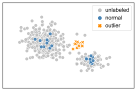
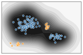
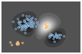
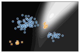
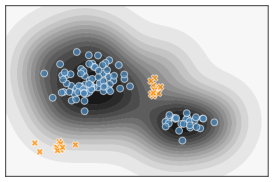
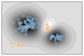
Anomaly detection (AD) (Chandola et al., 2009; Pimentel et al., 2014) is the task of identifying unusual samples in data. Typically AD methods attempt to learn a “compact” description of the data in an unsupervised manner assuming that most of the samples are normal (i.e., not anomalous). For example, in one-class classification (Moya et al., 1993; Schölkopf et al., 2001) the objective is to find a set of small measure which contains most of the data and samples not contained in that set are deemed anomalous. Shallow unsupervised AD methods such as the One-Class SVM (Schölkopf et al., 2001; Tax & Duin, 2004), Kernel Density Estimation (Parzen, 1962; Kim & Scott, 2012; Vandermeulen & Scott, 2013), or Isolation Forest (Liu et al., 2008) often require manual feature engineering to be effective on high-dimensional data and are limited in their scalability to large datasets. These limitations have sparked great interest in developing novel deep approaches to unsupervised AD (Erfani et al., 2016; Zhai et al., 2016; Chen et al., 2017; Ruff et al., 2018; Deecke et al., 2018; Ruff et al., 2019; Golan & El-Yaniv, 2018; Pang et al., 2019; Hendrycks et al., 2019a; b).
Unlike the standard unsupervised AD setting, in many real-world applications one may also have access to some verified (i.e., labeled) normal or anomalous samples in addition to the unlabeled data. Such samples could be hand labeled by a domain expert for instance. This leads to a semi-supervised AD problem: given (mostly normal but possibly containing some anomalous contamination) unlabeled samples and labeled samples , where and denote normal and anomalous samples respectively, the task is to learn a model that compactly characterizes the “normal class.”
The term semi-supervised anomaly detection has been used to describe two different AD settings. Most existing “semi-supervised” AD methods, both shallow (Muñoz-Marí et al., 2010; Blanchard et al., 2010; Chandola et al., 2009) and deep (Song et al., 2017; Akcay et al., 2018; Chalapathy & Chawla, 2019), only incorporate the use of labeled normal samples but not labeled anomalies, i.e. they are more precisely instances of Learning from Positive (i.e., normal) and Unlabeled Examples (LPUE) (Denis, 1998; Zhang & Zuo, 2008). A few works (Wang et al., 2005; Liu & Zheng, 2006; Görnitz et al., 2013) have investigated the general semi-supervised AD setting where one also utilizes labeled anomalies, however existing deep approaches are domain or data-type specific (Ergen et al., 2017; Kiran et al., 2018; Min et al., 2018).
Research on deep semi-supervised learning has almost exclusively focused on classification as the downstream task (Kingma et al., 2014; Rasmus et al., 2015; Odena, 2016; Dai et al., 2017; Oliver et al., 2018). Such semi-supervised classifiers typically assume that similar points are likely to be of the same class, this is known as the cluster assumption (Zhu, 2005; Chapelle et al., 2009). This assumption, however, only holds for the “normal class” in AD, but is crucially invalid for the “anomaly class” since anomalies are not necessarily similar to one another. Instead, semi-supervised AD approaches must find a compact description of the normal class while also correctly discriminating the labeled anomalies (Görnitz et al., 2013). Figure 1 illustrates the differences between various learning paradigms applied to AD on a toy example.
We introduce Deep SAD (Deep Semi-supervised Anomaly Detection) in this work, an end-to-end deep method for general semi-supervised AD. Our main contributions are the following:
-
•
We introduce Deep SAD, a generalization of the unsupervised Deep SVDD method (Ruff et al., 2018) to the semi-supervised AD setting.
-
•
We present an information-theoretic framework for deep AD, which can serve as an interpretation of our Deep SAD method and similar approaches.
-
•
We conduct extensive experiments in which we establish experimental scenarios for the general semi-supervised AD problem where we also introduce novel baselines.
2 An Information-theoretic View on Deep Anomaly Detection
The study of the theoretical foundations of deep learning is an active and ongoing research effort (Montavon et al., 2011; Tishby & Zaslavsky, 2015; Cohen et al., 2016; Eldan & Shamir, 2016; Neyshabur et al., 2017; Raghu et al., 2017; Zhang et al., 2017; Achille & Soatto, 2018; Arora et al., 2018; Belkin et al., 2018; Wiatowski & Bölcskei, 2018; Lapuschkin et al., 2019). One important line of research that has emerged is rooted in information theory (Shannon, 1948). In the supervised classification setting where one has input variable , latent variable (e.g., the final layer of a deep network), and output variable (i.e., the label), the well-known Information Bottleneck principle (Tishby et al., 1999; Tishby & Zaslavsky, 2015; Shwartz-Ziv & Tishby, 2017; Alemi et al., 2017; Saxe et al., 2018) provides an explanation for representation learning as the trade-off between finding a minimal compression of the input while retaining the informativeness of for predicting the label . Put formally, supervised deep learning seeks to minimize the mutual information between the input and the latent representation while maximizing the mutual information between and the classification task , i.e.
| (1) |
where is modeled by a deep network and the hyperparameter controls the trade-off between compression (i.e., complexity) and classification accuracy.
For unsupervised deep learning, due to the absence of labels and thus the lack of a clear task, other information-theoretic learning principles have been formulated. Of these, the Infomax principle (Linsker, 1988; Bell & Sejnowski, 1995; Hjelm et al., 2019) is one of the most prevalent and widely used principles. In contrast to (1), the objective of Infomax is to maximize the mutual information between the data and its latent representation :
| (2) |
This is typically done under some additional constraint or regularization on the representation with hyperparameter to obtain statistical properties desired for some specific downstream task. Examples where the Infomax principle has been applied include tasks such as independent component analysis (Bell & Sejnowski, 1995), clustering (Slonim et al., 2005; Ji et al., 2018), generative modeling (Chen et al., 2016; Hoffman & Johnson, 2016; Zhao et al., 2017; Alemi et al., 2018), and unsupervised representation learning in general (Hjelm et al., 2019).
We observe that the Infomax principle has also been applied in previous deep representations for AD. Most notably autoencoders (Rumelhart et al., 1986; Hinton & Salakhutdinov, 2006), which are the predominant approach to deep AD (Hawkins et al., 2002; Sakurada & Yairi, 2014; Andrews et al., 2016; Erfani et al., 2016; Zhai et al., 2016; Chen et al., 2017; Chalapathy & Chawla, 2019), can be understood as implicitly maximizing the mutual information via the reconstruction objective (Vincent et al., 2008) under some regularization of the latent code . Choices for regularization include sparsity (Makhzani & Frey, 2014), the distance to some latent prior distribution, e.g. measured via the KL divergence (Kingma & Welling, 2013; Rezende et al., 2014), an adversarial loss (Makhzani et al., 2015), or simply a bottleneck in dimensionality. Such restrictions for AD share the idea that the latent representation of the normal data should be in some sense “compact.”
As illustrated in Figure 1, a supervised (or semi-supervised) classification approach to AD only learns to recognize anomalies similar to those seen during training, due to the class cluster assumption (Chapelle et al., 2009). However, anything not normal is by definition an anomaly and thus anomalies do not have to be similar. This makes supervised (or semi-supervised) classification learning principles such as (1) ill-defined for AD. We instead build upon principle (2) to motivate a deep method for general semi-supervised AD, where we include the label information through a novel representation learning regularization objective that is based on entropy.
3 Deep Semi-supervised Anomaly Detection
In the following, we introduce Deep SAD, a deep method for general semi-supervised AD. To formulate our objective, we first briefly explain the unsupervised Deep SVDD method (Ruff et al., 2018) which we then generalize to the semi-supervised AD setting.
3.1 Unsupervised Deep SVDD and Entropy Minimization
For input space and output space , let be a neural network with hidden layers and corresponding set of weights . The objective of Deep SVDD is to train the neural network to learn a transformation that minimizes the volume of a data-enclosing hypersphere in output space centered on a predetermined point . Given (unlabeled) training samples , the One-Class Deep SVDD objective is
| (3) |
Penalizing the mean squared distance of the mapped samples to the hypersphere center forces the network to extract those common factors of variation which are most stable within the dataset. As a consequence normal data points tend to get mapped near the hypersphere center, whereas anomalies are mapped further away (Ruff et al., 2018). The second term is a standard weight decay regularizer.
Deep SVDD is optimized via SGD using backpropagation. For initialization, Ruff et al. (2018) first pre-train an autoencoder and then initialize the weights of the network with the converged weights of the encoder. After initialization, the hypersphere center is set as the mean of the network outputs obtained from an initial forward pass of the data. Once the network is trained, the anomaly score for a test point is given by the distance from to the center of the hypersphere:
| (4) |
We now argue that Deep SVDD may not only be interpreted in geometric terms as minimum volume estimation (Scott & Nowak, 2006), but also in probabilistic terms as entropy minimization over the latent distribution. For a latent random variable with covariance , pdf , and support , we have the following bound on entropy
| (5) |
which holds with equality iff is jointly Gaussian (Cover & Thomas, 2012). Assuming the latent distribution follows an isotropic Gaussian, with , we get
| (6) |
i.e. for a fixed dimensionality , the entropy of is proportional to its log-variance.
Now observe that the Deep SVDD objective (3) (disregarding weight decay regularization) is equivalent to minimizing the empirical variance and thus minimizes an upper bound on the entropy of a latent Gaussian. Since the Deep SVDD network is pre-trained on an autoencoding objective that implicitly maximizes the mutual information (Vincent et al., 2008), we may interpret Deep SVDD as following the Infomax principle (2) with the additional “compactness” objective that the latent distribution should have minimal entropy.
3.2 Deep SAD
We now introduce our method for deep semi-supervised anomaly detection: Deep SAD. Assume that, in addition to the unlabeled samples with , we also have access to labeled samples with where denotes known normal samples and known anomalies. We define our Deep SAD objective as follows:
| (7) |
We employ the same loss term as Deep SVDD for the unlabeled data in our Deep SAD objective and thus recover Deep SVDD (3) as the special case when there is no labeled training data available (). In doing this we also incorporate the assumption that most of the unlabeled data is normal.
For the labeled data, we introduce a new loss term that is weighted via the hyperparameter which controls the balance between the labeled and the unlabeled term. Setting puts more emphasis on the labeled data whereas emphasizes the unlabeled data. For the labeled normal samples (), we also impose a quadratic loss on the distances of the mapped points to the center , thus intending to overall learn a latent distribution which concentrates the normal data. Again, one might consider to emphasize labeled normal over unlabeled samples. For the labeled anomalies () in contrast, we penalize the inverse of the distances such that anomalies must be mapped further away from the center.111To ensure numerical stability, we add a machine epsilon (eps ) to the denominator of the inverse. Note that this is in line with the common assumption that anomalies are not concentrated (Schölkopf & Smola, 2002; Steinwart et al., 2005). In our experiments we found that simply setting yields a consistent and substantial performance improvement. A sensitivity analysis on is in Section 4.3.
We define the Deep SAD anomaly score again by the distance of the mapped point to the center as given in Eq. (4) and optimize our Deep SAD objective (7) via SGD using backpropagation. We provide a summary of the Deep SAD optimization procedure and further details in Appendix C.
In addition to the inverse squared norm loss we experimented with several other losses including the negative squared norm loss, negative robust losses, and the hinge loss. The negative squared norm loss, which is unbounded from below, resulted in an ill-posed optimization problem and caused optimization to diverge. Negative robust losses, such as the Hampel loss, introduce one or more scale parameters which are difficult to select or optimize in conjunction with the changing representation learned by the network. Like Ruff et al. (2018), we observed that the hinge loss was difficult to optimize and resulted in poorer performance. The inverse squared norm loss instead is bounded from below and smooth, which are crucial properties for losses used in deep learning (Goodfellow et al., 2016), and ultimately performed the best while remaining conceptually simple.
Following our insights on the connection between Deep SVDD and entropy minimization from Section 3.1, we may interpret our Deep SAD objective as modeling the latent distribution of normal data, , to have low entropy, and the latent distribution of anomalies, , to have high entropy. Minimizing the distances to the center (i.e., minimizing the empirical variance) for the mapped points of labeled normal samples () induces a latent distribution with low entropy for the normal data. In contrast, penalizing low variance via the inverse squared norm loss for the mapped points of labeled anomalies () induces a latent distribution with high entropy for the anomalous data. That is, the network must attempt to map known anomalies to some heavy-tailed distribution. We argue that such a model better captures the nature of anomalies, which can be thought of as being generated from an infinite mixture of distributions that are different from the normal data distribution, indubitably a distribution that has high entropy. Our objective notably does not impose any cluster assumption on the anomaly-generating distribution as is typically made in supervised or semi-supervised classification approaches (Zhu, 2005; Chapelle et al., 2009). We can express this interpretation in terms of principle (2) with an entropy regularization objective on the latent distribution:
| (8) |
To maximize the mutual information , Deep SAD also relies on autoencoder pre-training (Vincent et al., 2008; Ruff et al., 2018).
4 Experiments
We evaluate Deep SAD on MNIST, Fashion-MNIST, and CIFAR-10 as well as on classic AD benchmark datasets. We compare to shallow, hybrid, as well as deep unsupervised, semi-supervised and supervised competitors. We refer to other recent works (Ruff et al., 2018; Golan & El-Yaniv, 2018; Hendrycks et al., 2019a) for further comparisons between unsupervised deep AD methods.222Our code is available at: https://github.com/lukasruff/Deep-SAD-PyTorch
4.1 Competing Methods
We consider the OC-SVM (Schölkopf et al., 2001) and SVDD (Tax & Duin, 2004) with Gaussian kernel (which in this case are equivalent), Isolation Forest (Liu et al., 2008), and KDE (Parzen, 1962) for shallow unsupervised baselines. For deep unsupervised competitors, we consider well-established (convolutional) autoencoders and the state-of-the-art unsupervised Deep SVDD method (Ruff et al., 2018). To avoid confusion, we note again that some literature (Song et al., 2017; Chalapathy & Chawla, 2019) refer to the methods above as being “semi-supervised” if they are trained on only labeled normal samples. For general semi-supervised AD approaches that also take advantage of labeled anomalies, we consider the state-of-the-art shallow SSAD method (Görnitz et al., 2013) with Gaussian kernel. As mentioned earlier, there are no deep competitors for general semi-supervised AD that are applicable to general data types. To get a comprehensive comparison we therefore introduce a novel hybrid SSAD baseline that applies SSAD to the latent codes of autoencoder models. Such hybrid methods have demonstrated solid performance improvements over their raw feature counterparts on high-dimensional data (Erfani et al., 2016; Nicolau et al., 2016). We also include such hybrid variants for all unsupervised shallow competitors. To also compare to a deep semi-supervised learning method that targets classification as the downstream task, we add the well-known Semi-Supervised Deep Generative Model (SS-DGM) (Kingma et al., 2014) where we use the latent class probability estimate (normal vs. anomalous) as the anomaly score. To complete the full learning spectrum, we also include a fully supervised deep classifier trained on the binary cross-entropy loss.
In our experiments we deliberately grant the shallow and hybrid methods an unfair advantage by selecting their hyperparameters to maximize AUC on a subset (10%) of the test set to minimize hyperparameter selection issues. To control for architectural effects between the deep methods, we always use the same (LeNet-type) deep networks. Full details on network architectures and hyperparameter selection can be found in Appendices D and E. Due to space constraints, in the main text we only report results for methods which showed competitive performance and defer results for the underperforming methods in Appendix F.
4.2 Experimental Scenarios on MNIST, Fashion-MNIST, and CIFAR-10
Semi-supervised anomaly detection setup MNIST, Fashion-MNIST, and CIFAR-10 all have ten classes from which we derive ten AD setups on each dataset following previous works (Ruff et al., 2018; Chalapathy et al., 2018; Golan & El-Yaniv, 2018). In every setup, we set one of the ten classes to be the normal class and let the remaining nine classes represent anomalies. We use the original training data of the respective normal class as the unlabeled part of our training set. Thus we start with a clean AD setting that fulfills the assumption that most (in this case all) unlabeled samples are normal. The training data of the respective nine anomaly classes then forms the data pool from which we draw anomalies for training to create different scenarios. We compute the commonly used AUC measure on the original respective test sets using ground truth labels to make a quantitative comparison, i.e. for the normal class and for the respective nine anomaly classes. We rescale pixels to via min-max feature scaling as the only data pre-processing step.
Experimental scenarios We examine three scenarios in which we vary the following three experimental parameters: (i) the ratio of labeled training data , (ii) the ratio of pollution in the unlabeled training data with (unknown) anomalies, and (iii) the number of anomaly classes included in the labeled training data.
(i) Adding labeled anomalies In this scenario, we investigate the effect that including labeled anomalies during training has on detection performance to see the benefit of a general semi-supervised AD approach over other paradigms. To do this we increase the ratio of labeled training data by adding more and more known anomalies with to the training set. The labeled anomalies are sampled from one of the nine anomaly classes (). For testing, we then consider all nine remaining classes as anomalies, i.e. there are eight novel classes at testing time. We do this to simulate the unpredictable nature of anomalies. For the unlabeled part of the training set, we keep the training data of the respective normal class, which we leave unpolluted in this experimental setup, i.e. . We iterate this training set generation process per AD setup always over all the nine respective anomaly classes and report the average results over the ten AD setups nine anomaly classes, i.e. over 90 experiments per labeled ratio .
(ii) Polluted training data Here we investigate the robustness of the different methods to an increasing pollution ratio of the training set with unlabeled anomalies. To do so we pollute the unlabeled part of the training set with anomalies drawn from all nine respective anomaly classes in each AD setup. We fix the ratio of labeled training samples at where we again draw samples only from anomaly class in this scenario. We repeat this training set generation process per AD setup over all the nine respective anomaly classes and report the average results over the resulting 90 experiments per pollution ratio . We hypothesize that learning from labeled anomalies in a semi-supervised AD approach alleviates the negative impact pollution has on detection performance since similar unknown anomalies in the unlabeled data might be detected.
(iii) Number of known anomaly classes In the last scenario, we compare the detection performance at various numbers of known anomaly classes. In scenarios (i) and (ii), we always sample labeled anomalies only from one out of the nine anomaly classes (). In this scenario, we now increase the number of anomaly classes included in the labeled part of the training set. Since we have a limited number of anomaly classes (nine) in each AD setup, we expect the supervised classifier to catch up at some point. We fix the overall ratio of labeled training examples again at and consider a pollution ratio of for the unlabeled training data in this scenario. We repeat this training set generation process for ten seeds in each of the ten AD setups and report the average results over the resulting 100 experiments per number . For each seed, the classes are drawn uniformly at random from the nine respective anomaly classes.
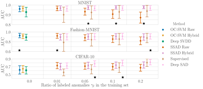
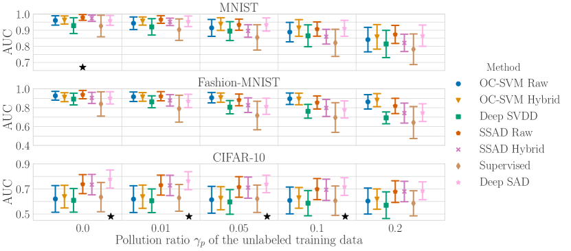
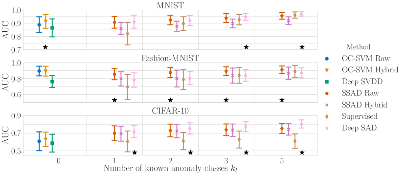
Results The results of scenarios (i)–(iii) are shown in Figures 2–4. In addition to the avg. AUC with st. dev., we report the outcome of Wilcoxon signed-rank tests (Wilcoxon, 1945) applied to the first and second best performing method to indicate statistically significant () differences in performance. Figure 2 demonstrates the benefit of our semi-supervised approach to AD especially on the most complex CIFAR-10 dataset, where Deep SAD performs best. Figure 2 moreover confirms that a supervised classification approach is vulnerable to novel anomalies at testing time when only little labeled training data is available. In comparison, Deep SAD generalizes to novel anomalies while also taking advantage of the labeled examples. Note that our novel hybrid SSAD baseline also performs well. Figure 3 shows that the detection performance of all methods decreases with increasing data pollution. Deep SAD proves to be most robust again especially on CIFAR-10. Finally, Figure 4 shows that the more diverse the labeled anomalies in the training set, the better the detection performance becomes. We can again see that the supervised method is very sensitive to the number of anomaly classes but catches up at some point as suspected. This does not occur with CIFAR-10, however, where labeled training samples seems to be insufficient for classification. Overall, we see that Deep SAD is particularly beneficial on the more complex data.
4.3 Sensitivity analysis
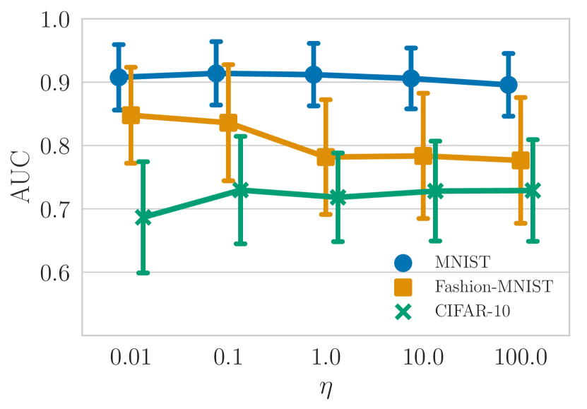
We run Deep SAD experiments on the ten AD setups described above on each dataset for to analyze the sensitivity of Deep SAD with respect to the hyperparameter . In this analysis, we set the experimental parameters to their default, , , and , and again iterate over all nine anomaly classes in every AD setup. The results shown in Figure 5 suggest that Deep SAD is fairly robust against changes of the hyperparameter .
In addition, we run experiments under the same experimental settings while varying the dimension of the output space to infer the sensitivity of Deep SAD with respect to the representation dimensionality, where we keep . The results are given in Figure 6 in Appendix A. There we also compare to our hybrid SSAD baseline, which was the strongest competitor. Interestingly we observe that detection performance increases with dimension , converging to an upper bound in performance. This suggests that one would want to set large enough to have sufficiently high mutual information before compressing to a compact characterization.
4.4 Classic Anomaly Detection Benchmark Datasets
In a final experiment, we also examine the detection performance of the various methods on some well-established AD benchmark datasets (Rayana, 2016). We run these experiments to evaluate the deep versus the shallow approaches on non-image datasets that are rarely considered in deep AD literature. Here we observe that the shallow kernel methods seem to have a slight edge on the relatively small, low-dimensional benchmarks. Nonetheless, Deep SAD proves competitive and the small differences observed might be explained by the advantage we grant the shallow methods in their hyperparameter selection. We give the full details and results in Appendix B.
Our results and other recent works (Ruff et al., 2018; Golan & El-Yaniv, 2018; Hendrycks et al., 2019a) overall demonstrate that deep methods are especially superior on complex data with hierarchical structure. Unlike other deep approaches (Ergen et al., 2017; Kiran et al., 2018; Min et al., 2018; Deecke et al., 2018; Golan & El-Yaniv, 2018), however, our Deep SAD method is not domain or data-type specific. Due to its good performance using both deep and shallow networks we expect Deep SAD to extend well to other data types.
5 Conclusion and Future Work
In this work we introduced Deep SAD, a deep method for general semi-supervised anomaly detection. Our method is a generalization of the unsupervised Deep SVDD method (Ruff et al., 2018) to the semi-supervised setting. The results of our experimental evaluation suggest that general semi-supervised anomaly detection should always be preferred whenever some labeled information on both normal samples or anomalies is available.
Moreover, we formulated an information-theoretic framework for deep anomaly detection based on the Infomax principle. Using this framework, we interpreted our method as minimizing the entropy of the latent distribution for normal data and maximizing the entropy of the latent distribution for anomalous data. We introduced this framework with the aim of forming a basis for new methods as well as rigorous theoretical analyses in the future, e.g. studying deep anomaly detection under the rate-distortion curve (Alemi et al., 2018).
Acknowledgments
LR acknowledges support by the German Ministry of Education and Research (BMBF) in the project ALICE III (01IS18049B). MK and RV acknowledge support by the German Research Foundation (DFG) award KL 2698/2-1 and by the German Ministry of Education and Research (BMBF) awards 031L0023A, 01IS18051A, and 031B0770E. AB is grateful for support by the National Research Foundation of Singapore, STEE-SUTD Cyber Security Laboratory, and the Ministry of Education, Singapore, under its program MOE2016-T2-2-154. NG acknowledges support by the German Ministry of Education and Research (BMBF) through the Berlin Center for Machine Learning (01IS18037I). KRM acknowledges partial financial support by the German Ministry of Education and Research (BMBF) under grants 01IS14013A-E, 01IS18025A, 01IS18037A, 01GQ1115 and 01GQ0850; Deutsche Forschungsgesellschaft (DFG) under grant Math+, EXC 2046/1, project-ID 390685689, and by the Technology Promotion (IITP) grant funded by the Korea government (No. 2017-0-00451, No. 2017-0-01779).
References
- Achille & Soatto (2018) Alessandro Achille and Stefano Soatto. Emergence of invariance and disentanglement in deep representations. Journal of Machine Learning Research, 19(1):1947–1980, 2018.
- Akcay et al. (2018) Samet Akcay, Amir Atapour-Abarghouei, and Toby P Breckon. GANomaly: Semi-supervised anomaly detection via adversarial training. In ACCV, pp. 622–637, 2018.
- Alemi et al. (2017) Alexander A Alemi, Ian Fischer, Joshua V Dillon, and Kevin Murphy. Deep variational information bottleneck. In ICLR, 2017.
- Alemi et al. (2018) Alexander A Alemi, Ben Poole, Ian Fischer, Joshua V Dillon, Rif A Saurous, and Kevin Murphy. Fixing a broken ELBO. In ICML, volume 80, pp. 159–168, 2018.
- Andrews et al. (2016) Jerone T A Andrews, Edward J Morton, and Lewis D Griffin. Detecting Anomalous Data Using Auto-Encoders. IJMLC, 6(1):21, 2016.
- Arora et al. (2018) Sanjeev Arora, Nadav Cohen, and Elad Hazan. On the optimization of deep networks: Implicit acceleration by overparameterization. In ICML, volume 80, pp. 244–253, 2018.
- Belkin et al. (2018) Mikhail Belkin, Siyuan Ma, and Soumik Mandal. To understand deep learning we need to understand kernel learning. In ICML, pp. 540–548, 2018.
- Bell & Sejnowski (1995) Anthony J Bell and Terrence J Sejnowski. An information-maximization approach to blind separation and blind deconvolution. Neural computation, 7(6):1129–1159, 1995.
- Blanchard et al. (2010) Gilles Blanchard, Gyemin Lee, and Clayton Scott. Semi-supervised novelty detection. Journal of Machine Learning Research, 11(Nov):2973–3009, 2010.
- Chalapathy & Chawla (2019) Raghavendra Chalapathy and Sanjay Chawla. Deep learning for anomaly detection: A survey. arXiv:1901.03407, 2019.
- Chalapathy et al. (2018) Raghavendra Chalapathy, Aditya Krishna Menon, and Sanjay Chawla. Anomaly detection using one-class neural networks. arXiv:1802.06360, 2018.
- Chandola et al. (2009) Varun Chandola, Arindam Banerjee, and Vipin Kumar. Anomaly Detection: A Survey. ACM Computing Surveys, 41(3):1–58, 2009.
- Chapelle et al. (2009) Olivier Chapelle, Bernhard Schölkopf, and Alexander Zien. Semi-supervised learning. IEEE Transactions on Neural Networks, 20(3):542–542, 2009.
- Chen et al. (2017) Jinghui Chen, Saket Sathe, Charu C Aggarwal, and Deepak S Turaga. Outlier Detection with Autoencoder Ensembles. In SDM, pp. 90–98, 2017.
- Chen et al. (2016) Xi Chen, Yan Duan, Rein Houthooft, John Schulman, Ilya Sutskever, and Pieter Abbeel. InfoGAN: Interpretable representation learning by information maximizing generative adversarial nets. In NIPS, pp. 2172–2180, 2016.
- Cohen et al. (2016) Nadav Cohen, Or Sharir, and Amnon Shashua. On the expressive power of deep learning: A tensor analysis. In COLT, volume 49, pp. 698–728, 2016.
- Cover & Thomas (2012) Thomas M Cover and Joy A Thomas. Elements of Information Theory. John Wiley & Sons, 2012.
- Dai et al. (2017) Zihang Dai, Zhilin Yang, Fan Yang, William W Cohen, and Ruslan R Salakhutdinov. Good semi-supervised learning that requires a bad gan. In NIPS, pp. 6510–6520, 2017.
- Deecke et al. (2018) Lucas Deecke, Robert A Vandermeulen, Lukas Ruff, Stephan Mandt, and Marius Kloft. Image anomaly detection with generative adversarial networks. In ECML-PKDD, 2018.
- Denis (1998) François Denis. PAC learning from positive statistical queries. In International Conference on Algorithmic Learning Theory, pp. 112–126, 1998.
- Eldan & Shamir (2016) Ronen Eldan and Ohad Shamir. The power of depth for feedforward neural networks. In COLT, volume 49, pp. 907–940, 2016.
- Erfani et al. (2016) Sarah M Erfani, Sutharshan Rajasegarar, Shanika Karunasekera, and Christopher Leckie. High-dimensional and large-scale anomaly detection using a linear one-class SVM with deep learning. Pattern Recognition, 58:121–134, 2016.
- Ergen et al. (2017) Tolga Ergen, Ali Hassan Mirza, and Suleyman Serdar Kozat. Unsupervised and semi-supervised anomaly detection with LSTM neural networks. arXiv:1710.09207, 2017.
- Glorot & Bengio (2010) Xavier Glorot and Yoshua Bengio. Understanding the difficulty of training deep feedforward neural networks. In AISTATS, pp. 249–256, 2010.
- Golan & El-Yaniv (2018) Izhak Golan and Ran El-Yaniv. Deep anomaly detection using geometric transformations. In NeurIPS, pp. 9758–9769, 2018.
- Goodfellow et al. (2016) Ian Goodfellow, Yoshua Bengio, and Aaron Courville. Deep Learning. MIT Press, 2016. http://www.deeplearningbook.org.
- Görnitz et al. (2013) Nico Görnitz, Marius Kloft, Konrad Rieck, and Ulf Brefeld. Toward supervised anomaly detection. Journal of Artificial Intelligence Research, 46:235–262, 2013.
- Hawkins et al. (2002) Simon Hawkins, Hongxing He, Graham Williams, and Rohan Baxter. Outlier Detection Using Replicator Neural Networks. In DaWaK, volume 2454, pp. 170–180, 2002.
- Hendrycks et al. (2019a) Dan Hendrycks, Mantas Mazeika, and Thomas G Dietterich. Deep anomaly detection with outlier exposure. In ICLR, 2019a.
- Hendrycks et al. (2019b) Dan Hendrycks, Mantas Mazeika, Saurav Kadavath, and Dawn Song. Using self-supervised learning can improve model robustness and uncertainty. In NeurIPS, pp. 15637–15648, 2019b.
- Hinton & Salakhutdinov (2006) Geoffrey E Hinton and Ruslan R Salakhutdinov. Reducing the Dimensionality of Data with Neural Networks. Science, 313(5786):504–507, 2006.
- Hjelm et al. (2019) R Devon Hjelm, Alex Fedorov, Samuel Lavoie-Marchildon, Karan Grewal, Adam Trischler, and Yoshua Bengio. Learning deep representations by mutual information estimation and maximization. In ICLR, 2019.
- Hoffman & Johnson (2016) Matthew D Hoffman and Matthew J Johnson. ELBO surgery: yet another way to carve up the variational evidence lower bound. In NIPS Workshop in Advances in Approximate Bayesian Inference, 2016.
- Ioffe & Szegedy (2015) Sergey Ioffe and Christian Szegedy. Batch Normalization: Accelerating Deep Network Training by Reducing Internal Covariate Shift. In ICML, pp. 448–456, 2015.
- Ji et al. (2018) Xu Ji, Joao F Henriques, and Andrea Vedaldi. Invariant information distillation for unsupervised image segmentation and clustering. arXiv:1807.06653, 2018.
- Kim & Scott (2012) JooSeuk Kim and Clayton D Scott. Robust kernel density estimation. Journal of Machine Learning Research, 13(Sep):2529–2565, 2012.
- Kingma & Ba (2015) Diederik P Kingma and Jimmy Ba. Adam: A Method for Stochastic Optimization. In ICLR, 2015.
- Kingma & Welling (2013) Diederik P Kingma and Max Welling. Auto-encoding variational bayes. In ICLR, 2013.
- Kingma et al. (2014) Diederik P Kingma, Shakir Mohamed, Danilo Jimenez Rezende, and Max Welling. Semi-supervised learning with deep generative models. In NIPS, pp. 3581–3589, 2014.
- Kiran et al. (2018) B Kiran, Dilip Thomas, and Ranjith Parakkal. An overview of deep learning based methods for unsupervised and semi-supervised anomaly detection in videos. Journal of Imaging, 4(2):36, 2018.
- Lapuschkin et al. (2019) Sebastian Lapuschkin, Stephan Wäldchen, Alexander Binder, Grégoire Montavon, Wojciech Samek, and Klaus-Robert Müller. Unmasking clever hans predictors and assessing what machines really learn. Nature communications, 10(1):1096, 2019.
- Linsker (1988) Ralph Linsker. Self-organization in a perceptual network. IEEE Computer, 21(3):105–117, 1988.
- Liu et al. (2008) Fei T Liu, Kai M Ting, and Zhi-Hua Zhou. Isolation Forest. In ICDM, pp. 413–422, 2008.
- Liu & Zheng (2006) Yi Liu and Yuan F Zheng. Minimum enclosing and maximum excluding machine for pattern description and discrimination. In ICPR, pp. 129–132, 2006.
- Makhzani & Frey (2014) Alireza Makhzani and Brendan Frey. K-sparse autoencoders. In ICLR, 2014.
- Makhzani et al. (2015) Alireza Makhzani, Jonathon Shlens, Navdeep Jaitly, Ian Goodfellow, and Brendan Frey. Adversarial autoencoders. arXiv:1511.05644, 2015.
- Min et al. (2018) Erxue Min, Jun Long, Qiang Liu, Jianjing Cui, Zhiping Cai, and Junbo Ma. SU-IDS: A semi-supervised and unsupervised framework for network intrusion detection. In International Conference on Cloud Computing and Security, pp. 322–334, 2018.
- Montavon et al. (2011) Grégoire Montavon, Mikio L Braun, and Klaus-Robert Müller. Kernel analysis of deep networks. Journal of Machine Learning Research, 12(Sep):2563–2581, 2011.
- Moya et al. (1993) Mary M Moya, Mark W Koch, and Larry D Hostetler. One-class classifier networks for target recognition applications. In Proceedings World Congress on Neural Networks, pp. 797–801, 1993.
- Muñoz-Marí et al. (2010) Jordi Muñoz-Marí, Francesca Bovolo, Luis Gómez-Chova, Lorenzo Bruzzone, and Gustavo Camp-Valls. Semi-Supervised One-Class Support Vector Machines for Classification of Remote Sensing Sata. IEEE Transactions on Geoscience and Remote Sensing, 48(8):3188–3197, 2010.
- Neyshabur et al. (2017) Behnam Neyshabur, Srinadh Bhojanapalli, David McAllester, and Nati Srebro. Exploring generalization in deep learning. In NIPS, pp. 5947–5956, 2017.
- Nicolau et al. (2016) Miguel Nicolau, James McDermott, et al. A hybrid autoencoder and density estimation model for anomaly detection. In International Conference on Parallel Problem Solving from Nature, pp. 717–726, 2016.
- Odena (2016) Augustus Odena. Semi-supervised learning with generative adversarial networks. arXiv:1606.01583, 2016.
- Oliver et al. (2018) Avital Oliver, Augustus Odena, Colin Raffel, Ekin D Cubuk, and Ian J Goodfellow. Realistic evaluation of deep semi-supervised learning algorithms. In NeurIPS, pp. 3235–3246, 2018.
- Pang et al. (2019) Guansong Pang, Chunhua Shen, and Anton van den Hengel. Deep anomaly detection with deviation networks. In KDD, pp. 353–362, 2019.
- Parzen (1962) E. Parzen. On Estimation of a Probability Density Function and Mode. The annals of mathematical statistics, 33(3):1065–1076, 1962.
- Pimentel et al. (2014) Marco AF Pimentel, David A Clifton, Lei Clifton, and Lionel Tarassenko. A review of novelty detection. Signal Processing, 99:215–249, 2014.
- Raghu et al. (2017) Maithra Raghu, Ben Poole, Jon Kleinberg, Surya Ganguli, and Jascha Sohl Dickstein. On the expressive power of deep neural networks. In ICML, volume 70, pp. 2847–2854, 2017.
- Rasmus et al. (2015) Antti Rasmus, Mathias Berglund, Mikko Honkala, Harri Valpola, and Tapani Raiko. Semi-supervised learning with ladder networks. In NIPS, pp. 3546–3554, 2015.
- Rayana (2016) Shebuti Rayana. ODDS library, 2016. URL http://odds.cs.stonybrook.edu.
- Rezende et al. (2014) Danilo Jimenez Rezende, Shakir Mohamed, and Daan Wierstra. Stochastic Backpropagation and Approximate Inference in Deep Generative Models. In ICML, volume 32, pp. 1278–1286, 2014.
- Ruff et al. (2018) Lukas Ruff, Robert A Vandermeulen, Nico Görnitz, Lucas Deecke, Shoaib A Siddiqui, Alexander Binder, Emmanuel Müller, and Marius Kloft. Deep one-class classification. In ICML, volume 80, pp. 4390–4399, 2018.
- Ruff et al. (2019) Lukas Ruff, Yury Zemlyanskiy, Robert Vandermeulen, Thomas Schnake, and Marius Kloft. Self-attentive, multi-context one-class classification for unsupervised anomaly detection on text. In ACL, pp. 4061–4071, 2019.
- Rumelhart et al. (1986) David E Rumelhart, Geoffrey E Hinton, and Ronald J Williams. Learning internal representations by error propagation. In Parallel Distributed Processing – Explorations in the Microstructure of Cognition, chapter 8, pp. 318–362. MIT Press, 1986.
- Sakurada & Yairi (2014) Mayu Sakurada and Takehisa Yairi. Anomaly detection using autoencoders with nonlinear dimensionality reduction. In Proceedings of the 2nd MLSDA Workshop, pp. 4, 2014.
- Saxe et al. (2018) Andrew Michael Saxe, Yamini Bansal, Joel Dapello, Madhu Advani, Artemy Kolchinsky, Brendan Daniel Tracey, and David Daniel Cox. On the information bottleneck theory of deep learning. In ICLR, 2018.
- Schölkopf & Smola (2002) Bernhard Schölkopf and Alex J Smola. Learning with Kernels. MIT press, 2002.
- Schölkopf et al. (2001) Bernhard Schölkopf, John C Platt, John Shawe-Taylor, Alex J Smola, and Robert C Williamson. Estimating the Support of a High-Dimensional Distribution. Neural computation, 13(7):1443–1471, 2001.
- Scott & Nowak (2006) Clayton D Scott and Robert D Nowak. Learning minimum volume sets. Journal of Machine Learning Research, 7(Apr):665–704, 2006.
- Shannon (1948) Claude Elwood Shannon. A mathematical theory of communication. Bell system technical journal, 27(3):379–423, 1948.
- Shwartz-Ziv & Tishby (2017) Ravid Shwartz-Ziv and Naftali Tishby. Opening the black box of deep neural networks via information. arXiv:1703.00810, 2017.
- Slonim et al. (2005) Noam Slonim, Gurinder Singh Atwal, Gašper Tkačik, and William Bialek. Information-based clustering. Proceedings of the National Academy of Sciences, 102(51):18297–18302, 2005.
- Song et al. (2017) Hongchao Song, Zhuqing Jiang, Aidong Men, and Bo Yang. A hybrid semi-supervised anomaly detection model for high-dimensional data. Computational Intelligence and Neuroscience, 2017.
- Steinwart et al. (2005) Ingo Steinwart, Don Hush, and Clint Scovel. A classification framework for anomaly detection. Journal of Machine Learning Research, 6(Feb):211–232, 2005.
- Tax & Duin (2004) David M J Tax and Robert P W Duin. Support Vector Data Description. Machine learning, 54(1):45–66, 2004.
- Tishby & Zaslavsky (2015) Naftali Tishby and Noga Zaslavsky. Deep learning and the information bottleneck principle. In 2015 IEEE Information Theory Workshop (ITW), pp. 1–5, 2015.
- Tishby et al. (1999) Naftali Tishby, Fernando C Pereira, and William Bialek. The information bottleneck method. In The 37th annual Allerton Conference on Communication, Control and Computing, pp. 368–377, 1999.
- Vandermeulen & Scott (2013) Robert A Vandermeulen and Clayton Scott. Consistency of robust kernel density estimators. In COLT, pp. 568–591, 2013.
- Vincent et al. (2008) Pascal Vincent, Hugo Larochelle, Yoshua Bengio, and Pierre-Antoine Manzagol. Extracting and composing robust features with denoising autoencoders. In ICML, pp. 1096–1103, 2008.
- Wang et al. (2005) Jigang Wang, Predrag Neskovic, and Leon N Cooper. Pattern classification via single spheres. In International Conference on Discovery Science, pp. 241–252. Springer, 2005.
- Wiatowski & Bölcskei (2018) Thomas Wiatowski and Helmut Bölcskei. A mathematical theory of deep convolutional neural networks for feature extraction. IEEE Transactions on Information Theory, 64(3):1845–1866, 2018.
- Wilcoxon (1945) Frank Wilcoxon. Individual comparisons by ranking methods. Biometrics Bulletin, 1(6):80–83, 1945.
- Zhai et al. (2016) Shuangfei Zhai, Yu Cheng, Weining Lu, and Zhongfei Zhang. Deep structured energy based models for anomaly detection. In ICML, volume 48, pp. 1100–1109, 2016.
- Zhang & Zuo (2008) Bangzuo Zhang and Wanli Zuo. Learning from positive and unlabeled examples: A survey. In Proceedings of the IEEE International Symposium on Information Processing, pp. 650–654, 2008.
- Zhang et al. (2017) Chiyuan Zhang, Samy Bengio, Moritz Hardt, Benjamin Recht, and Oriol Vinyals. Understanding deep learning requires rethinking generalization. In ICLR, 2017.
- Zhao et al. (2017) Shengjia Zhao, Jiaming Song, and Stefano Ermon. InfoVAE: Information maximizing variational autoencoders. arXiv:1706.02262, 2017.
- Zhu (2005) Xiaojin Zhu. Semi-supervised learning literature survey. Computer Sciences TR 1530, University of Wisconsin Madison, 2005.
Appendix A Additional Results on MNIST, Fashion-MNIST, and CIFAR-10
A.1 Sensitivity Analysis w.r.t Representation Dimensionality

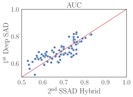
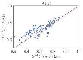
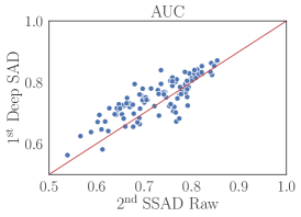
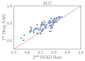
A.2 AUC Scatterplots of Best vs. Second Best Methods on CIFAR-10
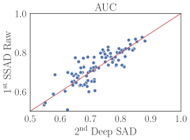
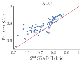
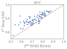
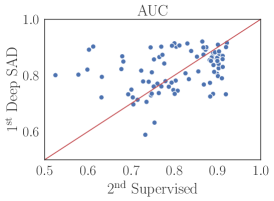
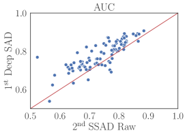
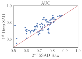
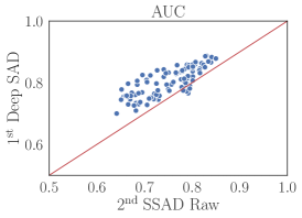
We provide AUC scatterplots in Figures 7–9 of the best (1st) vs. second best (2nd) performing methods in the experimental scenarios (i)–(iii) on the most complex CIFAR-10 dataset. If most points fall above the identity line, this is a very strong indication that the best method indeed significantly outperforms the second best, which often is the case for our Deep SAD method.


Appendix B Results on Classic Anomaly Detection Benchmark Datasets
| Dataset | #outliers (%) | ||
|---|---|---|---|
| arrhythmia | 452 | 274 | 66 (14.6%) |
| cardio | 1,831 | 21 | 176 (9.6%) |
| satellite | 6,435 | 36 | 2,036 (31.6%) |
| satimage-2 | 5,803 | 36 | 71 (1.2%) |
| shuttle | 49,097 | 9 | 3,511 (7.2%) |
| thyroid | 3,772 | 6 | 93 (2.5%) |
In this experiment, we examine the detection performance on some well-established AD benchmark datasets (Rayana, 2016) listed in Table 1. We do this to evaluate the deep against the shallow approaches also on non-image, tabular datasets that are rarely considered in the deep AD literature. For the evaluation, we consider random train-to-test set splits of 60:40 while maintaining the original proportion of anomalies in each set. We then run experiments for 10 seeds with and , i.e. 1% of the training set are labeled anomalies and the unlabeled training data is unpolluted. Since there are no specific different anomaly classes in these datasets, we have . We standardize features to have zero mean and unit variance as the only pre-processing step.
Table 2 shows the results of the competitive methods. We observe that the shallow kernel methods seem to perform slightly better on the rather small, low-dimensional benchmarks. Deep SAD proves competitive though and the small differences might be explained by the strong advantage we grant the shallow methods in the selection of their hyperparameters. We provide the complete table with the results from all methods in Appendix F
| OC-SVM | OC-SVM | Deep | SSAD | SSAD | Supervised | Deep | |
|---|---|---|---|---|---|---|---|
| Dataset | Raw | Hybrid | SVDD | Raw | Hybrid | Classifier | SAD |
| arrhythmia | 84.53.9 | 76.76.2 | 74.69.0 | 86.74.0⋆ | 78.35.1 | 39.29.5 | 75.98.7 |
| cardio | 98.50.3 | 82.89.3 | 84.83.6 | 98.80.3 | 86.35.8 | 83.29.6 | 95.01.6 |
| satellite | 95.10.2 | 68.64.8 | 79.84.1 | 96.20.3⋆ | 86.92.8 | 87.22.1 | 91.51.1 |
| satimage-2 | 99.40.8 | 96.72.1 | 98.31.4 | 99.90.1 | 96.82.1 | 99.90.1 | 99.90.1 |
| shuttle | 99.40.9 | 94.19.5 | 86.37.5 | 99.60.5 | 97.71.0 | 95.18.0 | 98.40.9 |
| thyroid | 98.30.9 | 91.24.0 | 72.09.7 | 97.91.9 | 95.33.1 | 97.82.6 | 98.60.9 |
Appendix C Optimization of Deep SAD
Our Deep SAD objective (7) is generally non-convex in the network weights which usually is the case in deep learning. For a computationally efficient optimization, we rely on (mini-batch) SGD to optimize the network weights using backpropagation. For improved generalization, we add weight decay regularization with hyperparameter to the objective. Algorithm 1 summarizes the Deep SAD optimization routine.
Using SGD allows Deep SAD to scale with large datasets as the computational complexity scales linearly in the number of training batches and computations in each batch can be parallelized (e.g., by training on GPUs). Moreover, Deep SAD has low memory complexity as a trained model is fully characterized by the final network parameters and no data must be saved or referenced for prediction. Instead, the prediction only requires a forward pass on the network which usually is just a concatenation of simple functions. This enables fast predictions for Deep SAD.
Initialization of the network weights We establish an autoencoder pre-training routine for initialization. That is, we first train an autoencoder that has an encoder with the same architecture as network on the reconstruction loss (mean squared error or cross-entropy). After training, we then initialize with the converged parameters of the encoder. Note that this is in line with the Infomax principle (2) for unsupervised representation learning (Vincent et al., 2008).
Initialization of the center After initializing the network weights , we fix the hypersphere center as the mean of the network representations that we obtain from an initial forward pass on the data (excluding labeled anomalies). We found SGD convergence to be smoother and faster by fixing center in the neighborhood of the initial data representations as also observed by Ruff et al. (2018). If sufficiently many labeled normal examples are available, using only those examples for a mean initialization would be another strategy to minimize possible distortions from polluted unlabeled training data. Adding center as a free optimization variable would allow a trivial “hypersphere collapse” solution for the fully unlabeled setting, i.e. for unsupervised Deep SVDD.
Preventing a hypersphere collapse A “hypersphere collapse” describes the trivial solution that neural network converges to the constant function , i.e. the hypersphere collapses to a single point. Ruff et al. (2018) demonstrate theoretical network properties that prevent such a collapse which we adopt for Deep SAD. Most importantly, network must have no bias terms and no bounded activation functions. We refer to Ruff et al. (2018) for further details. If there are sufficiently many labeled anomalies available for training, however, hypersphere collapse is not a problem for Deep SAD due to the opposing labeled and unlabeled objectives.
Appendix D Network Architectures
We employ LeNet-type convolutional neural networks (CNNs) on MNIST, Fashion-MNIST, and CIFAR-10, where each convolutional module consists of a convolutional layer followed by leaky ReLU activations with leakiness and -max-pooling. On MNIST, we employ a CNN with two modules, -filters followed by -filters, and a final dense layer of units. On Fashion-MNIST, we employ a CNN also with two modules, -filters and -filters, followed by two dense layers of and units respectively. On CIFAR-10, we employ a CNN with three modules, -filters, -filters, and -filters, followed by a final dense layer of units.
On the classic AD benchmark datasets, we employ standard MLP feed-forward architectures. On arrhythmia, a 3-layer MLP with -- units. On cardio, satellite, satimage-2, and shuttle a 3-layer MLP with -- units. On thyroid a 3-layer MLP with -- units.
For the (convolutional) autoencoders, we always employ the above architectures for the encoder networks and then construct the decoder networks symmetrically, where we replace max-pooling with simple upsampling and convolutions with deconvolutions.
Appendix E Details on Competing Methods
OC-SVM/SVDD The OC-SVM and SVDD are equivalent for the Gaussian/RBF kernel we employ. As mentioned in the main paper, we deliberately grant the OC-SVM/SVDD an unfair advantage by selecting its hyperparameters to maximize AUC on a subset (10%) of the test set to establish a strong baseline. To do this, we consider the RBF scale parameter and select the best performing one. Moreover, we always repeat this over -parameter and then report the best final result.
Isolation Forest (IF) We set the number of trees to and the sub-sampling size to , as recommended in the original work (Liu et al., 2008).
Kernel Density Estimator (KDE) We select the bandwidth of the Gaussian kernel from via 5-fold cross-validation using the log-likelihood score following (Ruff et al., 2018).
SSAD We also deliberately grant the state-of-the-art semi-supervised AD kernel method SSAD the unfair advantage of selecting its hyperparameters optimally to maximize AUC on a subset (10%) of the test set. To do this, we again select the scale parameter of the RBF kernel we use from and select the best performing one. Otherwise we set the hyperparameters as recommend by the original authors to , , , and (Görnitz et al., 2013).
(Convolutional) Autoencoder ((C)AE) To create the (convolutional) autoencoders, we symmetrically construct the decoders w.r.t. the architectures reported in Appenidx D, which make up the encoder parts of the autoencoders. Here, we replace max-pooling with simple upsampling and convolutions with deconvolutions. We train the autoencoders on the MSE reconstruction loss that also serves as the anomaly score.
Hybrid Variants To establish hybrid methods, we apply the OC-SVM, IF, KDE, and SSAD as outlined above to the resulting bottleneck representations given by the respective converged autoencoders.
Unsupervised Deep SVDD We consider both variants, Soft-Boundary Deep SVDD and One-Class Deep SVDD as unsupervised baselines and always report the better performance as the unsupervised result. For Soft-Boundary Deep SVDD, we optimally solve for the radius on every mini-batch and run experiments for . We set the weight decay hyperparameter to . For Deep SVDD, we always remove all the bias terms from a network to prevent a hypersphere collapse as recommended by the authors in the original work (Ruff et al., 2018).
Deep SAD We set and equally weight the unlabeled and labeled examples by setting if not reported otherwise.
SS-DGM We consider both the M2 and M1+M2 model and always report the better performing result. Otherwise we follow the settings as recommended in the original work (Kingma et al., 2014).
Note that we use the latent class probability estimate (normal vs. anomalous) of semi-supervised DGM as a natural choice for the anomaly score, and not the reconstruction error as used for unsupervised autoencoding models such as the (convolutional) autoencoder we consider. Such deep semi-supervised models designed for classification as the downstream task have no notion of out-of-distribution and again implicitly make the cluster assumption (Zhu, 2005; Chapelle et al., 2009) we refer to. Thus, semi-supervised DGM also suffers from overfitting to previously seen anomalies at training similar to the supervised model which explains its bad AD performance.
Supervised Deep Binary Classifier To interpret AD as a binary classification problem, we rely on the typical assumption that most of the unlabeled training data is normal by assigning to all unlabeled examples. Already labeled normal examples and labeled anomalies retain their assigned labels of and respectively. We train the supervised classifier on the binary cross-entropy loss. Note that in scenario (i), in particular, the supervised classifier has perfect, unpolluted label information but still fails to generalize as there are novel anomaly classes at testing.
SGD Optimization Details for Deep Methods We use the Adam optimizer with recommended default hyperparameters (Kingma & Ba, 2015) and apply Batch Normalization (Ioffe & Szegedy, 2015) in SGD optimization. For all deep approaches and on all datasets, we employ a two-phase (“searching” and “fine-tuning”) learning rate schedule. In the searching phase we first train with a learning rate for epochs. In the fine-tuning phase we train with for another epochs. We always use a batch size of 200. For the autoencoder, SS-DGM, and the supervised classifier, we initialize the network with uniform Glorot weights (Glorot & Bengio, 2010). For Deep SVDD and Deep SAD, we establish an unsupervised pre-training routine via autoencoder as explained in Appendix C, where we set the network to be the encoder of the autoencoder that we train beforehand.
Appendix F Complete Tables of Experimental Results
The following Tables LABEL:tab:1_known–LABEL:tab:odds_results_full list the complete experimental results of all the methods in all our experiments.