Estimation of Acoustic Impedance from Seismic Data using Temporal Convolutional Network

Abstract

In exploration seismology, seismic inversion refers to the process of inferring physical properties of the subsurface from seismic data. Knowledge of physical properties can prove helpful in identifying key structures in the subsurface for hydrocarbon exploration. In this work, we propose a workflow for predicting acoustic impedance (AI) from seismic data using a network architecture based on Temporal Convolutional Network by posing the problem as that of sequence modeling. The proposed workflow overcomes some of the problems that other network architectures usually face, like gradient vanishing in Recurrent Neural Networks, or overfitting in Convolutional Neural Networks. The proposed workflow was used to predict AI on Marmousi 2 dataset with an average $r^{2}$ coefficient of $91\%$ on a hold-out validation set.

1 Introduction

Reservoir characterization workflow involves the estimation of physical properties of the subsurface, like acoustic impedance (AI), from seismic data by incorporating knowledge of the well-logs. However, this is an extremely challenging task because in most seismic surveys due to the non-linearity of the mapping from seismic data to rock properties. Attempts to estimate physical properties from seismic data have been done using supervised machine learning algorithms, where the network is trained on pairs of seismic traces and their corresponding physical property traces from well-logs. The trained network is then used to obtain a map of physical properties for the entire seismic volume.

Recently, there has been a lot of work integrating machine learning algorithms in the seismic domain AlRegib et al., (2018). The literature shows successful applications of supervised machine learning algorithms to estimate petrophysical properties. For examples, Calder On-macas et al., (1999) used Artificial Neural Networks to predict velocity from prestack seismic gathers, Al-Anazi and Gates, (2012) used Support Vector Regression to predict porosity and permeability from core- and well-logs, Chaki et al., (2015) proposed novel preprocessing schemes based on algorithms like Fourier Transforms and Wavelet Decomposition before using the seismic attribute data to predict well-log properties. More recently, Lipari et al., (2018) used Generative Adversarial Networks (GANs) to map migrated seismic sections to their corresponding reflectivity section. Biswas et al., (2018) used Recurrent neural networks to predict stacking velocity from seismic offset gathers. Alfarraj and AlRegib, (2018) used Recurrent Neural Networks to invert seismic data for petrophysical properties by modeling seismic traces and well-logs as sequences. Das et al., (2018) used Convolutional Neural Network (CNNs) to predict p-impedance from normal incident seismic.

One challenge in all supervised learning schemes is to use a network that can train well on a limited amount of training data and can also generalize beyond the training data. Recurrent Neural Networks (RNNs) can subvert this problem by sharing their parameters across all time steps, and by using their hidden state to capture long term dependencies. However, they can be difficult to train because of the exploding/vanishing gradient problem. CNNs have great utility in capturing local trends in sequences, but in order to be able to capture long term dependencies, they need to have more layers (i.e, deeper networks), which in turn increase the number of learnable parameters. A network with a large number of parameters cannot be trained on limited training examples.

In this work, we used Temporal Convolutional Networks (TCN) to modeling traces as sequential data. The proposed network is trained in a supervised learning scheme on seismic data and their corresponding rock property traces (from well logs). The proposed workflow encapsulates the best features of both RNNs and CNNs as is captures long term trends in the data without requiring a large number of learnable parameters.

2 Temporal Convolutional Networks

One kind of sequence modeling task is to map a given a sequence of inputs $\{x(0),...,x(T-1)\}$ to a sequence of outputs ${y(0),...,y(T-1)}$ of the same length, where $T$ is the total number of time steps. The core idea is that this kind of a mapping described by the equation 1 can be represented by a neural network parameterized by $\Theta$ (i.e., $\mathcal{F}_{\Theta}$).

$$\hat{y}(t)=\mathcal{F}\left(x(0),\dots,x(t)\right)\forall t\in[0,T-1]$$ (1)

Convolutional Neural Networks (CNNs) have been used extensively for sequence modeling tasks like document classification Johnson and Zhang, (2015), machine translation Kalchbrenner et al., (2016), audio synthesisvan den Oord et al., (2016), and language modelingDauphin et al., (2016). More recently, Bai et al., (2018) performed a thorough comparison of canonical RNN architectures with their simple CNN architecture, which they call the Temporal Convolutional Network (TCN), and showed that the TCN was able to convincingly outperform RNNs on various sequence modeling tasks.

TCN is based on a series of dilated 1-D convolutions organized into Temporal Blocks. Each temporal block has the same basic structure. It has 2 convolution layers interspersed with weight normalization, dropout, and non-linearity layers. Figure 1 shows the organization of the various layers inside a temporal block.

Figure 1: The structure of a Temporal Block.

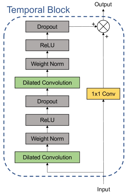
The weight normalization layers reparameterize the weights of the network. Each weight parameter is split into 2 parameters, one specifying its weight, and the other its direction. This kind of reparameterization, as Salimans and Kingma, (2016) show, helps improve convergence. The Dropout layers randomly zero out layer outputs, which helps prevent overfitting. The ReLU nonlinearity layers allow the network to learn more powerful representations. Each Convolution layer adds padding to the input so that the output is of the same size as input. There is also a skip connection from the input to the output of each temporal block. A distinguishing feature of the TCNs is their use of dilated convolutions, that allows the network to have a large receptive field, i.e., how many samples of the input contribute to each output. The size of the dilation factor increases exponentially at each temporal block. With regular convolution layers, one would have to use a very deep network to ensure the network has a large receptive field. On the other hand, using sequential dilated convolutions allows the network to look at large parts of the input without having to use many layers. This enables TCNs to capture long term trends better than RNNs. Skip connections in the TCN architecture help stabilize training in case of deeper networks. The concept of receptive field sits at the core of TCNs. Smaller convolution kernel sizes with fewer layers give the network a smaller receptive field, which allows it to capture local variations in sequential data well. However, such a network fails to capture the long term trends. On the other hand, larger kernel sizes with more layers give the network a large receptive field that makes it good at capturing long term trends, but not as good at preserving local variations. This is mainly due to the large number of successive convolutions which would dilute this information. This is also why adding skip connections to each residual block helps to overcome this drawback.

3 Problem Formulation

Let $\mathbf{X}=[\mathbf{x}^{1},\mathbf{x}^{2},...\mathbf{x}^{N}]$ be a set of post-stack seismic traces where $\mathbf{x}^{i}$ is the $i^{\text{th}}$ trace, and $\mathbf{Y}=[\mathbf{y}^{1},\mathbf{y}^{2},...\mathbf{y}^{N}]$ be the corresponding AI traces. A subset of X is inputted to the TCN in the forward propagation step. The network predicts the corresponding AI traces. The predicted AI traces are then compared to the true traces in the training dataset. The error between them is computed and is then used to compute the gradients. The gradients are then used to update the weights of the TCN in a step known as back-propagation. Repeated applications of forward propagation followed by backpropagation change the weights of the network to minimize the loss between the actual and predicted AI traces. We hypothesized that by treating both the stacked seismic trace $\textbf{x}^{n}$ and the corresponding AI trace $\textbf{y}^{n}$ as sequential data, we would be able to use the TCN architecture to learn the mapping $\mathcal{F}$ from seismic to AI. The training of the network can then be written mathematically as the following optimization problem:

$$\hat{\Theta}=\underset{\Theta}{\text{argmin}}~{}\frac{1}{N}\sum_{n=1}^{N}\mathcal{L}(\textbf{y}^{n},\mathcal{F}_{\Theta}(\textbf{x}^{n}))$$ (2)

where $\mathcal{L}$ is a distance function between the actual and predicted AI traces, $\mathcal{F}$ represents the forward propagation of the TCN on the input seismic to generate the corresponding predicted AI trace, and $\Theta$ represents the network weights.

4 Methodology

The network architecture used is shown in Figure 2. The seismic traces are passed through a series of temporal blocks. The output of the TCN is concatenated with the input seismic and then mapped to predicted AI using a linear layer. As discussed earlier, when using a larger kernel size with more layers, the network captures the low-frequency trend, but not the high-frequency fluctuations. On the other hand, with a smaller kernel size with fewer layers, the network captures the high frequencies but fails to capture the smoother trend. This is also why we concatenated the original seismic directly with the output of the TCN, so that any loss of high-frequency information due to successive convolutions in the temporal blocks might be compensated for. We found that this slightly improved the quality of our results. We experimented with different kernel sizes and number of layers, and found the numbers reported in Figure 2 worked best in terms of capturing both high- and low-frequency contents.

Figure 2: TCN architecture for predicting AI. The TCN consists of a series of 6 temporal blocks, the input and output channels for each specified in parentheses.

4.1 Training the network

There is a total of 2721 seismic and corresponding AI traces from the Marmousi model over a total length of 17000m. We sampled both the seismic section and the model at intervals of 937m, to obtain a total of 19 training traces ($\leq 1\%$ of the total number of traces). We chose Mean Square Error (MSE) as the loss function. Adam was used as the optimizer with a learning rate of 0.001 and a weight decay of 0.0001. We used a dropout of 0.2, kernel size of 5, and 6 temporal blocks. The TCN internally also uses weight normalization to improve training and speed up convergence. We trained the network for 2941 epochs, which took about 5 minutes to train on a NVIDIA GTX 1050 GPU. Once the network had been trained, inference on the whole seismic section was fast and took only a fraction of a second.

5 Results and Discussion

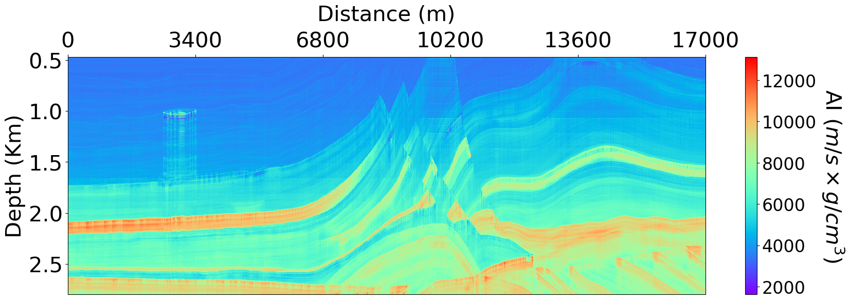
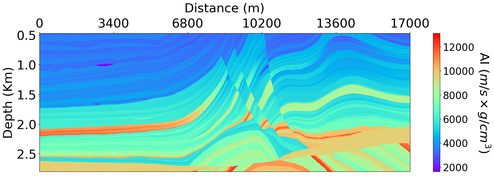
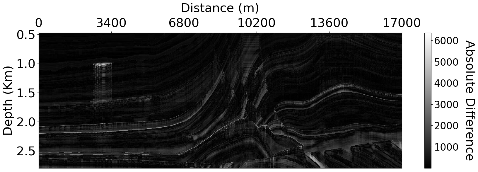
Figure 3 shows the predicted and actual AI, along with the absolute difference between the two. The predicted and actual AI sections show a high degree of visual similarity. The TCN is able to delineate most of the major structures. The difference image also shows that most of the discrepancy lies at the edge boundaries, which is because of sudden transitions in AI that the network is not accurately able to predict.

(a) Predicted AI

(b) True AI

(c) Absolute Difference

Figure 3: Comparison of the predicted and true Acoustic impedance sections of the Marmousi 2 model along with the absolute difference

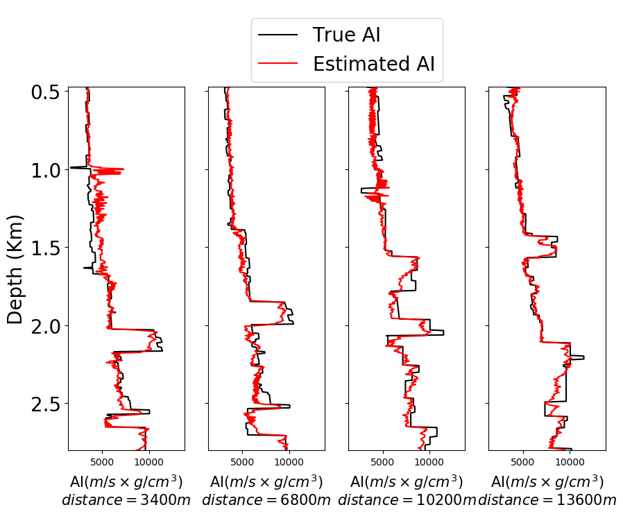
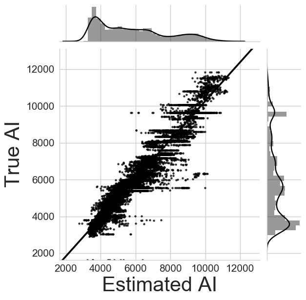
We also show traces at 3400m, 6800m, 10200m, and 13600m, respectively in Figure 4. As can be seen, the AI and estimated traces at each location agree with each other to a large extent. Figure 5 shows a scatter plot of the true and estimated AI. The scatter plot show that there is a strong linear correlation between the true and estimated AI sections.

Figure 4: Comparison of the predicted and true Acoustic impedance traces at selected locations along the horizontal axis.

Figure 5: Scatter Plot of the true and estimated AI

For a quantitative evaluation of the results, we computed the Pearson’s Correlation coefficient (PCC) and the coefficient of determination between estimated and true AI traces. PCC is a measure of the overall linear correlation between two traces. The coefficient of determination ($r^{2}$) is a measure of goodness of fit between two traces. The averaged values are shown in Table 1 for the training dataset and for the entire section (labeled as validation data). As can be seen, both the training and validation traces report a high value for the PCC and $r^{2}$ coefficients which confirms that the network was able to learn to predict AI from seismic traces well and to generalize beyond the training data.

Metric	Training	Validation
PCC	0.96	0.96
$r^{2}$	0.91	0.91

Table 1: Performance metrics for both the training and validation datasets.

6 Conclusion

In this work, we proposed a novel scheme of predicting acoustic impedance from seismic data using a Temporal Convolutional Network. The results were demonstrated on the Marmousi 2 model. The proposed workflow was trained on 19 training traces, and was then used to predict Acoustic Impedance for the entire Mamrousi model. Quantitative evaluation of the predicted AI (PCC $\approx 0.96$, and $r^{2}\approx 0.91$) shows great promise of the proposed workflow for acoustic impedance prediction. Even though the proposed workflow has been used for AI estimation in this paper, it can be used to predict any other property as well. Indeed, Temporal Convolutional Networks can be adapted to any problem that requires mapping one sequence to another.

7 Acknowledgements

This work is supported by the Center for Energy and Geo Processing (CeGP) at Georgia Institute of Technology and King Fahd University of Petroleum and Minerals (KFUPM).

References

- Al-Anazi and Gates, (2012) Al-Anazi, A., and I. Gates, 2012, Support vector regression to predict porosity and permeability: Effect of sample size: Computers & Geosciences, 39, 64 – 76.
- Alfarraj and AlRegib, (2018) Alfarraj, M., and G. AlRegib, 2018, Petrophysical property estimation from seismic data using recurrent neural networks, in SEG Technical Program Expanded Abstracts 2018: Society of Exploration Geophysicists, 2141–2146.
- AlRegib et al., (2018) AlRegib, G., M. Deriche, Z. Long, H. Di, Z. Wang, Y. Alaudah, M. A. Shafiq, and M. Alfarraj, 2018, Subsurface structure analysis using computational interpretation and learning: A visual signal processing perspective: IEEE Signal Processing Magazine, 35, 82–98.
- Bai et al., (2018) Bai, S., J. Z. Kolter, and V. Koltun, 2018, An empirical evaluation of generic convolutional and recurrent networks for sequence modeling: CoRR, abs/1803.01271.
- Biswas et al., (2018) Biswas, R., A. Vassiliou, R. Stromberg, and M. Sen, 2018, Stacking velocity estimation using recurrent neural network: , 2241–2245.
- Calder On-macas et al., (1999) Calder On-macas, C., M. Sen, and P. Stoffa, 1999, Automatic nmo correction and velocity estimation by a feedforward neural network: GEOPHYSICS, 63.
- Chaki et al., (2015) Chaki, S., A. Routray, and W. K. Mohanty, 2015, A novel preprocessing scheme to improve the prediction of sand fraction from seismic attributes using neural networks: IEEE Journal of Selected Topics in Applied Earth Observations and Remote Sensing, 8, 1808–1820.
- Das et al., (2018) Das, V., A. Pollack, U. Wollner, and T. Mukerji, 2018, Convolutional neural network for seismic impedance inversion, in SEG Technical Program Expanded Abstracts 2018: 2071–2075.
- Dauphin et al., (2016) Dauphin, Y. N., A. Fan, M. Auli, and D. Grangier, 2016, Language modeling with gated convolutional networks: CoRR, abs/1612.08083.
- Johnson and Zhang, (2015) Johnson, R., and T. Zhang, 2015, Semi-supervised convolutional neural networks for text categorization via region embedding, in Advances in Neural Information Processing Systems 28: Curran Associates, Inc., 919–927.
- Kalchbrenner et al., (2016) Kalchbrenner, N., L. Espeholt, K. Simonyan, A. van den Oord, A. Graves, and K. Kavukcuoglu, 2016, Neural machine translation in linear time: CoRR, abs/1610.10099.
- Lipari et al., (2018) Lipari, V., F. Picetti, P. Bestagini, and S. Tubaro, 2018, A generative adversarial network for seismic imaging applications: Presented at the .
- Salimans and Kingma, (2016) Salimans, T., and D. P. Kingma, 2016, Weight normalization: A simple reparameterization to accelerate training of deep neural networks: CoRR, abs/1602.07868.
- van den Oord et al., (2016) van den Oord, A., S. Dieleman, H. Zen, K. Simonyan, O. Vinyals, A. Graves, N. Kalchbrenner, A. W. Senior, and K. Kavukcuoglu, 2016, Wavenet: A generative model for raw audio: CoRR, abs/1609.03499.