Rapid noise prediction models for serrated leading and trailing edges

Abstract

Leading- and trailing-edge serrations have been widely used to reduce the leading- and trailing-edge noise in applications such as contra-rotating fans and large wind turbines. Recent studies show that these two noise problems can be modelled analytically using the Wiener-Hopf method. However, the resulting models involve infinite-interval integrals that cannot be evaluated analytically, and consequently implementing them poses practical difficulty. This paper develops easily-implementable noise prediction models for flat plates with serrated leading and trailing edges, respectively. By exploiting the fact that high-order modes are cut-off and adjacent modes do not interfere in the far field except at sufficiently high frequencies, an infinite-interval integral involving two infinite sums is approximated by a single straightforward sum. Numerical comparison shows that the resulting models serve as excellent approximations to the original models. Good agreement is also achieved when the leading-edge model predictions are compared with experimental results for sawtooth serrations of various root-to-tip amplitudes. Importantly, the models developed in this paper can be evaluated robustly in a very efficient manner. For example, a typical far-field noise spectrum can be calculated within milliseconds for both the trailing- and leading-edge noise models on a standard desktop computer. Due to their efficiency and ease of numerical implementation, these models are expected to be of particular importance in applications where a numerical optimization is likely to be needed.

1 Introduction

Airfoil noise is important in many applications such as contra-rotating fans and large wind turbines. It often involves more than one noise generation mechanism [1, 6]. Of particular relevance are the leading-edge (LE) noise and the turbulent boundary-layer trailing-edge (TE) noise. LE noise is due to the scattering of velocity fluctuations of the incoming flow by the leading-edge of an airfoil, therefore it is common in applications with multi-row rotors/stators where the wake flow due the front row impinges on the downstream blades leading to strong flow-structure interactions, such as in jet engines and contra-rotating fans. TE noise, on the other hand, is generated when a turbulent boundary layer convects past and then gets scattered by the trailing edge of an airfoil [16]. It is thus common in applications with highly turbulent boundary layers, such as wind turbines.

One of the early research works on LE noise was conducted by Graham [13], where similarity rules were established for the unsteady aerodynamic loading of the airfoil due to sinusoidal gusts at subsonic speed. Following Graham, Amiet [1] investigated the acoustic response of an airfoil subject to sinusoidal incoming gusts. Amiet used the Schwarzschild method and related the far-field sound Power Spectral Density (PSD) to the wavenumber spectral density of the vertical velocity fluctuations of the incoming turbulent flow. With an accurate model for the turbulence wavenumber spectral density, Amiet’s approach has been shown to work well and become an important method for following studies.

A serrated LE has been proposed as one of the most promising approaches to reduce LE noise [7, 12, 31, 15, 29], and extensive research has been carried out to study its noise reduction performance and mechanisms. This includes experimental studies such as those by Hansen et al. [15] and Narayanan et al. [29], numerical investigations carried out by Lau et al. [21], Kim et al. [20] and Turner and Kim [35], and analytical examinations such as those by Lyu and Azarpeyvand [23] and Ayton and Chaitanya [4].

Similarly, TE serrations have been widely used as an effective way of reducing TE noise. A large bulk of literature on this is experimental work. These include studies by Dassen et al. [11], Chong et al. [10], Moreau and Doolan [28], Oerlemans et al. [30], Gruber et al. [14], Chong and Vathylakis [9], Leon et al. [22], etc. Numerical techniques have also been widely used to study the TE serrations as a way of reducing TE noise, see for example those by Jones and Sandberg [19], Sanjose et al. [33] and van der Velden et al. [36]. A number of authors have also conducted analytical studies. Some of the early analytical works include those by Howe [17, 18], where a tailored Green’s function was used to predict the far-field sound generated by flat plates with sinusoidal and sawtooth serrations, respectively. However, Howe’s model dramatically overpredicted the sound reduction achieved by using TE serrations. Howe’s approach was later used by Azarpeyvand et al. [5] to study the noise reduction characteristics of other serration geometries. The recent work by Lyu et al. [25, 24], on the other hand, used Amiet’s approach and extended Amiet’s model [2, 34] for a straight trailing edge to the serrated case. The results showed that the principal noise reduction mechanism was due to the destructive interference and the predicted noise reduction was more realistic compared to experimental results.

Although the TE noise and LE noise are due to different noise generation mechanisms, mathematically they bear a striking similarity, hence, the techniques used to model the two problems are expected be similar to each other. For example, recent work [3, 4] shows that both the serrated LE noise and TE noise can be modelled analytically using the Wiener-Hopf method. This approach has shown good agreement with experiments for LE noise [4]. However, both the LE and TE solutions involve an infinite-interval integral, which makes their implementations both difficult and error-prone.

In this paper, we address this issue. By exploiting the fact that high-order modes are cut-off and little coupling between expanded modes occurs except at very high frequencies, we replace the infinite-interval integral that involves two infinite sums with one straightforward sum. The simplified model takes a particularly concise form when the serration wavelength is small compared to the transformed acoustic wavelength. The final results can therefore be easily implemented numerically in a robust and efficient manner.

This paper is structured as follows. Section 2 shows the essential analytical steps to reach the final results for both the LE and TE noise problems, respectively. Section 3 presents a comparison between the approximated results obtained in this paper and those obtained from the full analytical solutions. The following section uses the simplified leading-edge model to compare with the leading-edge noise spectra observed in experiments. The final section concludes this paper and lists directions for future work.

2 The leading-edge and trailing-edge noise models

As mentioned in Section 1, the TE and LE noise problems bear a striking similarity between each other. In either case, to allow the analytical derivation to continue, the serrated airfoil is often assumed to be a semi-infinite plate [1, 32, 4, 23, 25] placed in a uniform incoming flow of constant density $\tilde{\rho}$ and velocity $\tilde{U}$ at zero angle of attack, as shown in figure 1. The speed of sound is denoted by $\tilde{c}_{0}$. In the rest of this paper, the serration wavelength is used to normalized the length dimension, while $\tilde{\rho}$ and $\tilde{U}$ are used to non-dimensionalize other dynamic variables such as the velocity potential and pressure. In this paper, we restrict our attention to periodic leading-edge and trailing-edge serrations. Because the geometric parameters are normalized by the serration wavelength, the serrations have a period $1$. The normalized root-to-tip length is given by $2h$. Let $x$, $y$, $z$ denote the streamwise, spanwise and normal to the plate directions, respectively, and the coordinate origin is fixed in the middle between the root and tip. In such a coordinate frame, the serration profile can be described by $x=hF(y)$, where $F(y)$ is a single-valued function that has a maximum value $1$ and minimum value $-1$. Moreover, we require $1$ to be the smallest period. Other than these constraints, the function $F(y)$ is arbitrary.

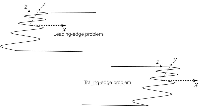
Figure 1: Schematic illustrations of the simplified leading-edge and trailing-edge noise problems. The two problems bear a striking similarity between each other.

Figure 1 shows the similarity between the simplified leading-edge and trailing-edge noise problems due to coordinate symmetry. Despite this symmetry, the physics they represent is quite different. For the leading-edge problem, the unsteady flow fluctuations, due to the incoming turbulence convected by the mean flow, are scattered into sound near the leading edge of the flat plate, whereas in the trailing-edge problem the source of scattering is the turbulence beneath turbulent boundary layers. The boundary conditions required by these two problems are therefore quite different. As such, we need to discuss them separately.

2.1 The leading-edge noise problem

When the turbulence in the mean flow passes the leading edge, a scattered potential flow is induced. The scattered potential ensures that appropriate boundary conditions are satisfied. In the leading-edge noise problem, the vertical velocity fluctuation of the incoming turbulence is of primary concern. The turbulence in the mean flow consists of a wide range of time and length scales. However, one can always perform a Fourier Transformation on the incoming vertical velocity field, such that it can be written as

$$w_{i}=\int_{-\infty}^{\infty}\hat{w}_{0}(\omega,k_{2})\mathrm{e}^{\mathrm{i}(-\omega t+k_{1}x+k_{2}y)}\mathrm{d}k_{2},$$ (1)

where $t$ denotes time, $\hat{w}_{0}$ the velocity fluctuation in the $z$ direction, $\omega$ the angular frequency and $k_{1}$ and $k_{2}$ the wavenumbers in the streamwise and spanwise directions, respectively. The turbulence is assumed to be frozen and convects downstream at a non-dimensional speed of $1$. Therefore, one has $k_{1}=\omega$.

Let $\phi_{s}$ denote this scattered velocity potential. One can show that $\phi_{s}$ satisfies the convective wave equation

$$\nabla^{2}\phi_{s}-M^{2}\left(\frac{\partial}{\partial t}+\frac{\partial}{\partial x}\right)^{2}\phi_{s}=0,$$ (2)

where $M=\tilde{U}/\tilde{c}_{0}$. To ensure that the normal velocity on the plate vanishes, we require

$$\left.\frac{\partial\phi_{s}}{\partial z}\right|_{z=0}=-w_{i},\quad x>hF(y).$$ (3)

The scattering problem is anti-symmetric across $z=0$, therefore we also have

$$\left.\phi_{s}\right|_{z=0}=0,\quad x<hF(y).$$ (4)

This mixed boundary condition problem can be solved using the Wiener-Hopf method [4, 27]. For the sake of brevity we omit the details of the solving procedure. Interested readers are referred to Ayton and Chaitanya [4] and the appendix of Lyu et al. [27]. Here we only give the results in the acoustical far-field as

$$p(\omega,r,\theta,y)\approx\int_{-\infty}^{\infty}H_{l}(\omega,\boldsymbol{x},k_{2})\hat{w}_{0}(\omega,k_{2})\mathrm{d}k_{2},$$ (5)

where

$$H_{l}(\omega,\boldsymbol{x},k_{2})=\frac{\mathrm{e}^{\mathrm{i}\pi/4}}{\sqrt{\pi}} \mathrm{e}^{-\mathrm{i}kMx/\beta^{2}}\cos\frac{\theta}{2}$$ (6)

$$\sum_{n=-\infty}^{\infty}\frac{\frac{k_{1}}{\beta^{2}}-\kappa_{n}\cos\theta}{\bar{k}_{1}-\kappa_{n}\cos\theta}\frac{1}{\sqrt{\bar{k}_{1}+\kappa_{n}}}\frac{\mathrm{e}^{\mathrm{i}\kappa_{n}r}}{\sqrt{r}}\mathrm{e}^{\mathrm{i}\chi_{n}y}E_{n}(-\kappa_{n}\cos\theta).$$

In equation 6, $r$, $\theta$ and $y$ denote, respectively, the radial, polar and axial axes of the stretched cylindrical coordinate system $(x/\beta,y,z)$, i.e. $y$ denotes the axial axis and $\theta$ is the polar angle to the stretched axis $x/\beta$ in the $(x/\beta,z)$ plane ($\theta=0$ corresponds to the $x/\beta$ axis) and $r=\sqrt{(x/\beta)^{2}+z^{2}}$. In addition, one has $k=\omega M$, $\beta=\sqrt{1-M^{2}}$, $\bar{k}_{1}=k_{1}/\beta$, $\chi_{n}=k_{2}+2n\pi$, $\kappa_{n}=\sqrt{k^{2}-\chi_{n}^{2}}$ and

$$E_{n}(-\kappa_{n}\cos\theta)=\int_{0}^{1}\mathrm{e}^{\mathrm{i}(\bar{k}_{1}-\kappa_{n}\cos\theta)\bar{h}F(\eta)}\mathrm{e}^{-\mathrm{i}2n\pi\eta}\mathrm{d}\eta,$$ (7)

where $\bar{h}=h/\beta$.

Since the incoming turbulence is statistically stationary, the far-field sound is best formulated statistically. Routine procedure shows that the far-field sound PSD is given by

$$\Psi(\omega,r,\theta,y)=\lim_{T\to\infty}\frac{\pi}{T}p(\omega,r,\theta,y)p^{\ast}(\omega,r,\theta,y),$$ (8)

where $2T$ is the time interval used to performed temporal Fourier Transformation to obtain $p$ and the asterisk denotes the complex conjugate. Substituting equations 5 into 8, we can show that

$$\Psi(\omega,r,\theta,y)\approx \frac{1}{\pi r}\cos^{2}\frac{\theta}{2}$$ (9)

$$\times\int_{-\infty}^{\infty}\Pi_{l}(\omega,k_{2})\sum_{n=-\infty}^{\infty}\frac{\frac{k_{1}}{\beta^{2}}-\kappa_{n}\cos\theta}{\bar{k}_{1}-\kappa_{n}\cos\theta}\frac{E_{n}(-\kappa_{n}\cos\theta)}{\sqrt{\bar{k}_{1}+\kappa_{n}}}\mathrm{e}^{\mathrm{i}\chi_{n}y}\mathrm{e}^{\mathrm{i}\kappa_{n}r}$$

$$\times\sum_{m=-\infty}^{\infty}\left[\frac{\frac{k_{1}}{\beta^{2}}-\kappa_{m}\cos\theta}{\bar{k}_{1}-\kappa_{m}\cos\theta}\frac{E_{m}(-\kappa_{m}\cos\theta)}{\sqrt{\bar{k}_{1}+\kappa_{m}}}\mathrm{e}^{\mathrm{i}\chi_{m}y}\mathrm{e}^{\mathrm{i}\kappa_{m}r}\right]^{\ast}\mathrm{d}k_{2},$$

where $\Pi_{l}(\omega,k_{2})$ is the wavenumber frequency spectrum of the vertical velocity fluctuations due to the incoming turbulence.

Experiments and theories have shown that narrow serrations (a small serration wavelength) are more effective than wide serrations in reducing the LE noise [29, 23]. This is related to the spanwise correlation length of the incoming gust, hence to the integral scale of the incoming turbulence. A detailed discussion was given by Lyu and Azarpeyvand [23] and Lyu et al. [27]. Consequently, for practical usage, we only need to restrict our attention to narrow serrations. Under the assumption of narrow serrations, equation 9 can be further simplified. First, we only need to investigate the case where both $\kappa_{n}$ and $\kappa_{m}$ are real, because otherwise the exponential term $\mathrm{e}^{\mathrm{i}\kappa_{n}r}(\mathrm{e}^{\mathrm{i}\kappa_{m}r})^{\ast}$ causes the whole term to decay exponentially in the far field. Noting that $\kappa_{n}=\sqrt{\bar{k}^{2}-\chi_{n}^{2}}$, we see that $\kappa_{n}$ is real only when $-\bar{k}<\chi_{n}<\bar{k}$. Because we restrict to the case where the serration wavelength is small, in the frequency range of interest we may have $\bar{k}<\pi$. It is, therefore, permissible to have

$$\mathrm{e}^{\mathrm{i}\kappa_{n}r}(\mathrm{e}^{\mathrm{i}\kappa_{m}r})^{\ast}=\delta_{nm}\mathrm{sgn}(\Re(\kappa_{n})),$$ (10)

where $\mathrm{sgn}(0)=0$ and $\mathrm{sgn}(x)=\pm 1$ when $\pm x>0$. Note equation 10 shows that its right hand side vanishes when $\kappa_{n}$ is imaginary. This implies that

$$\Psi(r,\theta,y)\sim \frac{1}{\pi r}\cos^{2}\frac{\theta}{2}\sum_{n=-\infty}^{\infty}\int_{-\infty}^{\infty}\Pi_{l}(\omega,k_{2})$$ (11)

$$\times\left|(\frac{k_{1}}{\beta^{2}}-\kappa_{n}\cos\theta)\frac{E_{n}(-\kappa_{n}\cos\theta)}{(-\kappa_{n}\cos\theta+\bar{k}_{1})\sqrt{\bar{k}_{1}+\kappa_{n}}}\right|^{2}\mathrm{sgn}(\Re(\kappa_{n}))\mathrm{d}k_{2}.$$

Second, in light of the fact that $\kappa_{n}$ is real only when $-\bar{k}<\chi_{n}<\bar{k}$ and the serration wavelength is small, the integrand does not vanish only when $-2n\pi-\bar{k}\leq k_{2}\leq-2n\pi+\bar{k}$. Over such a typically small range of $k_{2}$, the integrand of equation 5 does not vary significantly due to its algebraic dependence on $k_{2}$ (provided the Mach number is not close to $1$). Hence we can factor the $k_{2}$ dependence out of the integral, and change the integration interval to $-2n\pi-\bar{k}$ to $-2n\pi+\bar{k}$, without causing significant errors. Upon doing so, equation 5 simplifies to

$$\Psi(r,\theta,y)\sim\frac{2\bar{k}}{\pi r}\cos^{2}\frac{\theta}{2}\frac{(\frac{k_{1}}{\beta^{2}}-\bar{k}\cos\theta)^{2}}{(\bar{k}_{1}-\bar{k}\cos\theta)^{2}(\bar{k}_{1}+\bar{k})}\sum_{n=-\infty}^{\infty}\Pi_{l}(\omega,2n\pi)\left|E_{n}(-\bar{k}\cos\theta)\right|^{2}.$$ (12)

Equation 12 is obtained by assuming the serrations are narrow. It would of course be useful to know how narrow can be regarded as appropriate. This can be obtained from the criterion that $\bar{k}<\pi$ (recall lengths are non-dimensionlised by the serration wavelength). In fact, when $\pi<\bar{k}\leq 2\pi$, the overlap between adjacent modes is still rather weak, therefore it is often permissible to assume that the approximation is still valid when $\bar{k}\leq 2\pi$. It is clear that this inequality depends only on the (dimensional) serration wavelength, (dimensional) acoustic wavenumber and Mach number. This is likely to be satisfied in practical applications. To put this into perspective, let us take an typical example applicable in the wind industry for an airfoil of chord $1$ m placed in a mean flow of Mach number $0.2$. The serration wavelength is around $2$ cm while the serration root-to-tip is around $10$ cm. The inequality will therefore hold for a frequency up to $17$ KHz, which is near the upper limit of the audible frequency range. Thus, our approximation is valid for the full range of practical interest in this case.

2.2 The trailing-edge noise problem

When the turbulent boundary layer convects past the trailing edge of a flat plate, a scattered pressure field is induced. In a similar manner, we may write the wavenumber frequency spectrum of the wall pressure fluctuations beneath the boundary layer as

$$p_{i}=\int_{-\infty}^{\infty}\hat{p}_{0}(\omega,k_{2})\mathrm{e}^{\mathrm{i}(-\omega t+k_{1}x+k_{2}y)}\mathrm{d}k_{2},$$ (13)

where relevant quantities are defined in a similar way as those defined in section 2.1, except here $\hat{p}_{0}$ is the amplitude of the Fourier component of wall pressure fluctuations and $k_{1}=\omega/\alpha$, where $\alpha$ is a constant. In other words, these pressure fluctuations are assumed to convect at a speed of $\alpha$. Here we use a typical value of $\alpha\approx 0.7$ [25].

Let $p_{s}$ denote the scattered pressure field, which satisfies the convective wave equation, i.e.

$$\nabla^{2}p_{s}-M^{2}\left(\frac{\partial}{\partial t}+\frac{\partial}{\partial x}\right)^{2}p_{s}=0.$$ (14)

The boundary conditions are such that the normal velocity on the plate vanishes, i.e.

$$\left.\frac{\partial p_{s}}{\partial z}\right|_{z=0}=0,\quad x<hF(y),$$ (15)

and that the scattered pressure is $0$ on the semi-infinite plane $z=0$ and $x>hF(y)$, i.e.

$$\Delta p_{s}|_{z=0}=-p_{i},\quad x>hF(y),$$ (16)

where $\Delta p_{s}$ denotes the pressure jump across the plate. The solution $p_{s}$ satisfying equation 2 subject to the boundary conditions shown in equations 15 and 16 can be found (see for example Ayton [3]) to be

$$p_{s}(\omega,r,\theta,y)\approx\int_{-\infty}^{\infty}H_{t}(\omega,\boldsymbol{x},k_{2})\hat{p}_{0}(\omega,k_{2})\mathrm{d}k_{2},$$ (17)

where

$$H_{t}(\omega,\boldsymbol{x},k_{2})=\frac{\mathrm{e}^{\mathrm{i}\pi/4}}{\sqrt{\pi}} \mathrm{e}^{-\mathrm{i}kMx/\beta^{2}}\sin\frac{\theta}{2}$$ (18)

$$\times\sum_{n=-\infty}^{\infty}\frac{\sqrt{-\bar{k}_{1}-\kappa_{n}}}{2\mathrm{i}(\bar{k}_{1}-\kappa_{n}\cos\theta)}\frac{\mathrm{e}^{\mathrm{i}\kappa_{n}r}}{\sqrt{r}}\mathrm{e}^{\mathrm{i}\chi_{n}y}E_{n}(-\kappa_{n}\cos\theta),$$

where $r$, $\theta$ are defined similar to those shown in Section 2.1. In addition, $\chi_{n}$ and $\kappa_{n}$ are defined the same as those in Section 2.1. However, we now define $\bar{k}_{1}=(k_{1}+(kM-k_{1}M^{2}))/\beta$ and

$$E_{n}(-\kappa_{n}\cos\theta)=\int_{0}^{1}\mathrm{e}^{\mathrm{i}(\bar{k}_{1}-\kappa_{n}\cos\theta)\bar{h}F(\eta)}\mathrm{e}^{-\mathrm{i}2n\pi\eta}\mathrm{d}\eta,$$ (19)

where $\bar{h}$ is similarly defined as $h/\beta$. Note here that the definitions of $k_{1}$ and $\bar{k}_{1}$ in this trailing-edge noise problem are different from those in the leading-edge noise problem.

In a very similar manner, the far-field sound PSD can be approximated, upon assuming the serration wavelength is sufficiently small such that $\bar{k}<\pi$, to be

$$\Psi (r,\theta,y)\sim\frac{1}{4\pi r}\sin^{2}\frac{\theta}{2}$$ (20)

$$\times\sum_{n=-\infty}^{\infty}\int_{-\infty}^{\infty}\Pi_{t}(\omega,k_{2})\left|\frac{\sqrt{-\bar{k}_{1}-\kappa_{n}}}{(\bar{k}_{1}-\kappa_{n}\cos\theta)}E_{n}(-\kappa_{n}\cos\theta)\right|^{2}\mathrm{sgn}(\Re(\kappa_{n}))\mathrm{d}k_{2},$$

where $\Pi_{t}(\omega,k_{2})$ denotes the wall pressure fluctuations wavenumber frequency spectrum beneath the turbulent boundary layer close to the trailing edge. Equation 20 can be further simplified by replacing the integral with a simple sum to be

$$\Psi(r,\theta,y)\sim\frac{\bar{k}}{2\pi r}\sin^{2}\frac{\theta}{2}\frac{\bar{k}_{1}+\bar{k}}{(\bar{k}_{1}-\bar{k}\cos\theta)^{2}}\sum_{n=-\infty}^{\infty}\Pi_{t}(\omega,2n\pi)\left|E_{n}(-\bar{k}\cos\theta)\right|^{2}.$$ (21)

It is worth noting equation 21 bears a striking similarity to equation 2.59 in the work of Lyu et al. [25]. The fact that two completely different approaches lead to consistent results of the same form shows that the essential physics are captured in both models. These two equations show that higher-order modes are still cut-on and contribute to the far-field (the earlier argument in Ayton [3] that higher-order modes were neglected in the model of Lyu et al. [25] was not an accurate statement).

3 Comparison with exact solutions

In Section 2, we reduce the complex original model to a straightforward sum and simplify the result significantly when the serrations are sufficiently narrow (i.e. serration wavelength is small compared to the transformed acoustic wavelength). In this section, to assess how accurate the approximations are, we perform a direction comparison between the full and the simplified solutions. Firstly, we choose to compare the solutions for LE serrations of a sawtooth profile as an illustration.

3.1 The leading-edge noise problem

To enable this comparison, we need a realistic wavenumber spectrum $\Pi_{l}(\omega,k_{2})$ to model the incoming turbulence. There are a number of empirical models available. As an illustration, we use the one developed from Von Kármàn spectrum. Based on this, it can be shown that $\Pi_{l}(\omega,k_{2})$, i.e. the wavenumber frequency spectrum of the incoming vertical fluctuation velocity, can be written as [1, 26, 23]

$$\Pi_{l}(\omega,k_{2})=\frac{4\textrm{TI}^{2}}{9\pi k_{e}^{2}}\frac{\hat{k}_{1}^{2}+\hat{k}_{2}^{2}}{(1+\hat{k}_{1}^{2}+\hat{k}_{2}^{2})^{7/3}},$$ (22)

where TI denotes the turbulent intensity and $k_{e}$, $\hat{k}_{1}$ and $\hat{k}_{2}$ are given by

$$k_{e}=\frac{\sqrt{\pi}\Gamma(5/6)}{L_{t}\Gamma(1/3)},\quad\hat{k}_{1}=\frac{k_{1}}{k_{e}},\quad\hat{k}_{2}=\frac{k_{2}}{k_{e}}.$$ (23)

In the above equations, $L_{t}$ is the integral scale of the turbulence (also normalized by the serration wavelength) and $\Gamma(x)$ is the Gamma function.

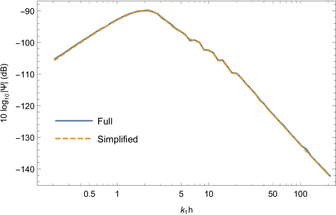
Figure 2: Comparison of predicted LE noise spectra from the full and simplified models: $M=0.18$, $\mathrm{TI}=0.025$, $h=5$, $L_{t}=0.3$, $r=30$, $\theta=90^{\circ}$ and $y=0$.

In order to put equation 22 into perspective, we require a realistic set of physical parameters of the incoming flow. For the sake of convenience, we use those given in previous experiments [29, 23], where $M=0.18$, $\textrm{TI}=0.025$ and $L_{t}=0.3$. As an illustrative example, we use sawtooth serrations with $h=5$. The observer distance is fixed at $r=30$ in the plane of $y=0$, but the observer angle is varied from $\theta=90^{\circ}$ to $20^{\circ}$. The far-field PSDs are evaluated from equations 9 and 12, respectively.

The comparison of the predicted noise spectra at $\theta=90^{\circ}$ is shown in figure 2. The solid line is obtained from the full solution, i.e. equation 9, while the dashed line is from the simplified solution, i.e. equation 12. It is clear that the two solutions agree excellently well with each other over the entire frequency range of interest. We choose $h=5$ because this represents sharp serrations where the approximation is the least accurate. At such a large value of $h$ we can hardly see the difference between the full and simplified solutions. We can therefore expect at least similar, if not better, agreement for smaller values of $h$.

Figure 2 is for a fixed observer at $90^{\circ}$ above the leading edge. Figure 3 shows the predicted noise spectra for the observer at $\theta=45^{\circ}$. The agreement is similar to that shown in figure 2, and the simplified model serves as an excellent approximation to the fully integrated solution. Figure 4 shows the simplified and full spectra when $\theta=20^{\circ}$, and the agreement continues to be very good.

It is worth mentioning, however, the computational costs are very different for the two solutions. For the full integral solution given by equation 9, it takes around one hour and a half to obtain the noise spectrum at a single observer location, whereas on average only $5$ ms is needed for the simplified model given by equation 12. The simplified model is faster than the original model by a factor of around $720,000$. More importantly, since no numerical integration of irregular integrands is involved, the computation is much more robust.

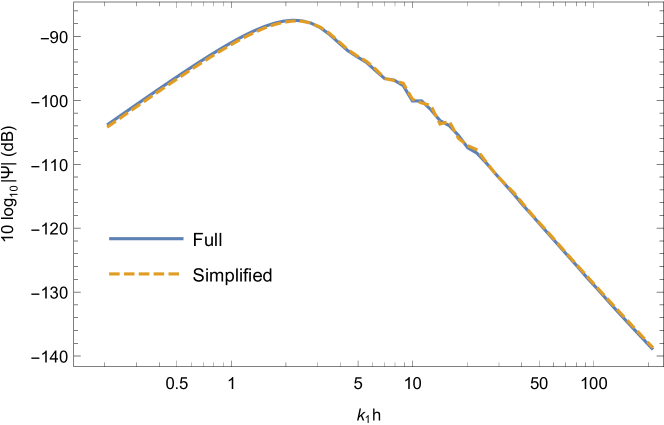
Figure 3: Comparison of predicted LE noise spectra from the full and simplified models: $M=0.18$, $\mathrm{TI}=0.025$, $h=5$, $L_{t}=0.3$, $r=30$, $\theta=45^{\circ}$ and $y=0$.

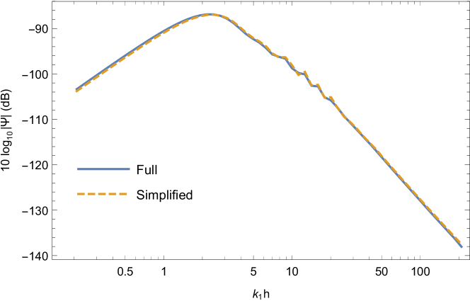
Figure 4: Comparison of predicted LE noise spectra from the full and simplified models: $M=0.18$, $\mathrm{TI}=0.025$, $h=5$, $L_{t}=0.3$, $r=30$, $\theta=20^{\circ}$ and $y=0$.

3.2 The trailing-edge noise problem

We now compare the approximated model to the full model for the TE noise problem. Similarly, the wall pressure wavenumber spectrum needs to be modelled. As an illustrative example, it suffices to choose Chase’s model [8, 25], i.e.

$$\Pi_{t}(\omega,k_{2})=\frac{4C_{m}v^{\ast 4}\delta^{4}k_{1}^{2}}{\alpha\left[(k_{1}^{2}+k_{2}^{2})\delta^{2}+\chi^{2}\right]^{2}},$$ (24)

where $C_{m}\approx 0.1533$, $v^{\ast}\approx 0.03$, $\chi\approx 1.33$, and $\delta$ denotes the non-dimensional boundary layer thickness. In this paper, we let $\delta$ take an approximate value of $1.01$, which corresponds to a realistic non-dimensional boundary layer thickness for a dimensional chord length of $1$ m when the serration wavelength is $0.02$ m.

To enable a direct comparison between the approximated and full results, we again use a sawtooth serration profile with $h=5$. The observer distance is fixed to be $r=30$ in the plane of $y=0$, and the observer angle is varied from $\theta=90^{\circ}$ to $20^{\circ}$. The predicted far-field spectra are plotted using the full solution based on equation 17 and the approximated solution shown in equation 21, respectively.

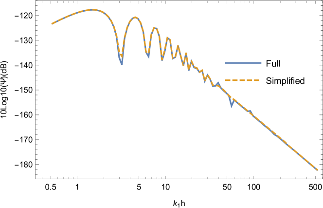
Figure 5: Comparison of predicted TE noise spectra from the full and simplified models: $M=0.1$, $h=5$, $\delta=1.01$, $r=30$, $\theta=90^{\circ}$ and $y=0$.

The comparison of the noise spectra at $\theta=90^{\circ}$ is shown in figure 5. As we can see the approximated solution agrees with the full solution with virtually no difference over the entire frequency range. Note that when $k_{1}h$ is close to $500$, $\bar{k}$ is slightly larger than $2\pi$. But the difference between the two lines is still hardly observable. Therefore, the condition $\bar{k}<2\pi$, although likely to be satisfied in most practical cases, may be further relaxed in practice.

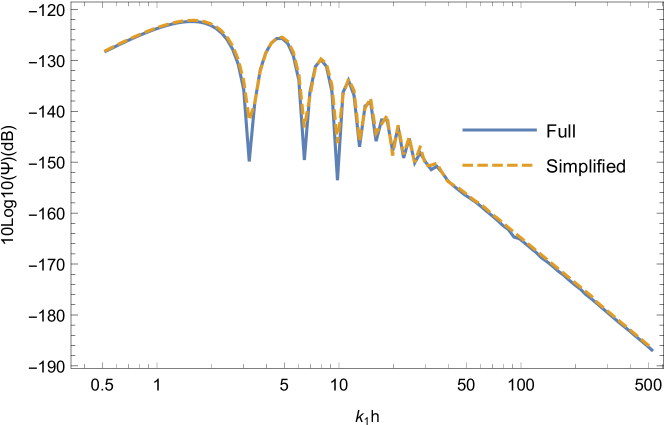
Figure 6: Comparison of predicted TE noise spectra from the full and simplified models: $M=0.1$, $h=5$, $\delta=1.01$, $r=30$, $\theta=45^{\circ}$ and $y=0$.

Figure 5 shows the comparison of the predicted spectra for $\theta=45^{\circ}$. The agreement continues to be very good, except slight disagreement occurring near the minima of the oscillation frequencies. The strong oscillations predicted by the models are due to the large value of $h$, i.e. the use of sharp serrations, leading to strong destructive interference (in experiments, however, these large dips are unlikely to be observed since the turbulence within the boundary layer is not strictly frozen). We choose this large value to examine how the simplified model works in the least accurate case. Had we used smaller values of $h$, these oscillations would have disappeared [3].

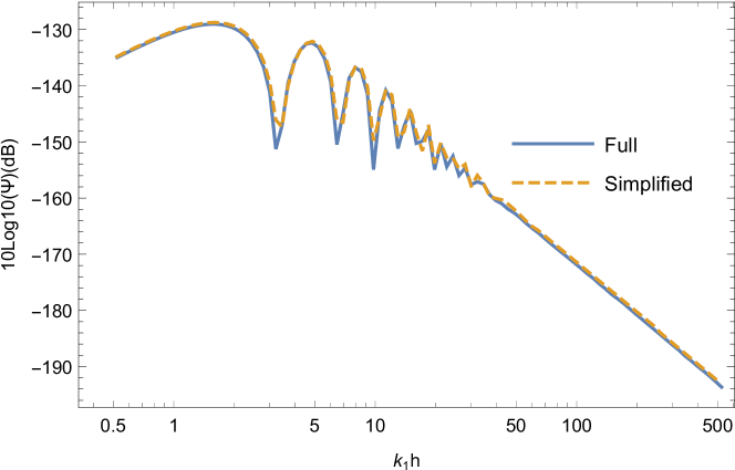
Figure 7: Comparison of predicted TE noise spectra from the full and simplified models: $M=0.1$, $h=5$, $\delta=1.01$, $r=30$, $\theta=20^{\circ}$ and $y=0$.

Figure 7 shows the two predicted spectra when $\theta=20^{\circ}$. The agreement continues to be very good over the entire frequency range of interest. Although the two spectra are virtually identical, the computational costs in obtaining them are, as those observed in the LE noise problem, strikingly different: while the full solution demands an hour for computing a single spectrum, the simplified model on average only needs a few milliseconds. In summary, the approximated solution serves as an efficient model for the TE noise problem. More importantly, the simplified TE noise model can be easily implemented and the computation is very robust, while the numerical integration in the full solution is prone to error due to the non-smooth behaviour of the integrand.

4 Comparison with experiments

Results from these simplified models can be directly compared with experimental data. Due to the similar nature of approximation, it suffices to focus on the leading-edge model. We choose to compare with the recent experimental results reported in Ayton and Chaitanya [4] and use the sawtooth serration as an example.

The experiment was carried out in the acoustic wind tunnel at the Institute of Sound and Vibration of Southampton University. The test facility features a $8\text{ m}\times 8\text{ m}\times 8\text{ m}$ anechoic chamber and a low-speed wind tunnel with a nozzle of $150\text{ mm}\times 450\text{ mm}$. More details on the test facility can be found in Ayton and Chaitanya [4]. Flat plates with serrated leading edges were placed $150\text{ mm}$ downstream from the nozzle exit. The serrations had a wavelength of $25\text{ mm}$, but the half root-to-tip amplitude was varied from $6.25\text{ mm}$ to $25\text{ mm}$. Therefore, the corresponding $h$ was varied from $1/4$ and $1$.

Free stream turbulence was generated by a rectangular grid of $630\text{ mm}\times 690\text{ mm}$ inside the contraction section located $75\text{ cm}$ upstream from the nozzle exit. The dimensionless turbulence spectrum $\Pi_{l}(\omega,k_{2})$ was characterised using the Liepmann model, i.e.

$$\Pi_{l}(\omega,k_{2})=\frac{3\mathrm{TI}^{2}L_{t}^{2}}{4\pi}\frac{L_{t}^{2}(k_{1}^{2}+k_{2}^{2})}{(1+L_{t}^{2}(k_{1}^{2}+k_{2}^{2}))^{5/2}},$$ (25)

where $\mathrm{TI}$ and $L_{t}$ were, as defined in section 3.1, the turbulence intensity and streamwise integral length scale, respectively. With equation 25, equation 12 can be quickly evaluated and the results can be compared with the noise spectra obtained in the experiment. These are presented in figures 8 to 10. To have an intuitive understanding of the frequency and amplitude, noise spectra are shown in their dimensional forms.

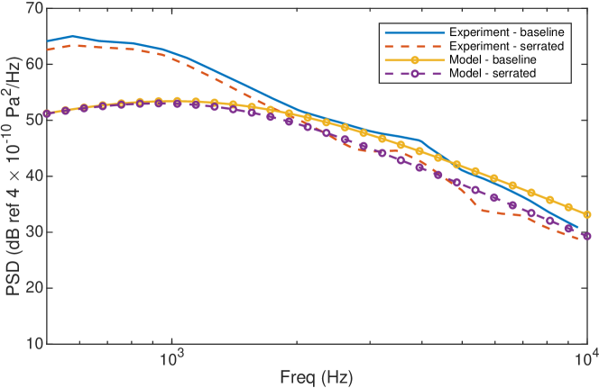
Figure 8: Comparison of the noise spectra between model prediction and experimental measurements when $h=1/4$.

We start comparing the model and experimental results for the short serration, i.e. for $h=1/4$. The far-field noise spectra are presented in figure 8. Both the serrated and baseline ($h=0$) spectra are shown. It is well known that in leading-edge noise experiments low-frequency noise is dominated by jet noise. Therefore, we do not make a direct comparison for frequencies less than $2000$ Hz. Good agreement is achieved, however, in the frequency range of $2000$ to $10000$ Hz for the baseline spectra. This shows that the simplified model works well for straight edges. In addition, the model predicts that a noise reduction of around $3$ dB can be achieved by using the short serration of $h=1/4$. The experimental data agree with such a prediction very well.

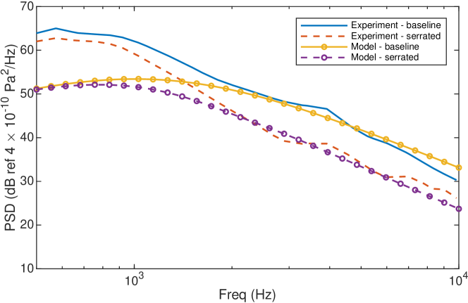
Figure 9: Comparison of the noise spectra between model prediction and experimental measurements when $h=1/2$.

Figure 9 shows the comparison for $h=1/2$. As can be seen, using the longer serration results in a higher noise reduction of up to $8$ dB in the experiment. The model can capture this change accurately and the resulting spectrum for the serrated edge agrees very well with that observed in the experiment. This is not surprising given that the simplified model agrees with the full solution to a high degree of accuracy.

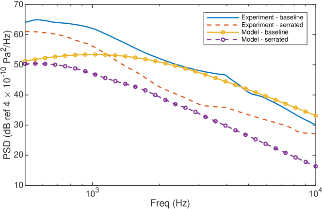
Figure 10: Comparison of the noise spectra between model prediction and experimental measurements when $h=1$.

Figure 10 shows the comparison for the long serration, i.e. for $h=1$. We expect an even greater noise reduction due to the use of serrations, and this is confirmed by the experiment, which shows a noise reduction of up to more than $10$ dB. However, the predicted noise reduction is around $15$ dB. The model therefore underpredicts the noise emitted by flat plates with long leading-edge serrations. However, this is not due to the failure of the simplified model, but rather due to neglecting contribution of trailing-edge noise, which occurs in the experiment and begins to dominate for when leading-edge noise is sufficiently suppressed. It has been shown by Ayton and Chaitanya [4] that adding in a trailing-edge noise model to the prediction results in good agreement with the experimental spectrum, however, as we are concerned with verifying the simplified models in this section, we have excluded the contribution of TE noise here. Figures 8 and 10 show that the simplified model serves as an accurate approximation to the full solution, which is both computationally expensive and error-prone. The simplified model overcomes these two issues and is therefore both efficient and robust.

5 Conclusion and future work

This paper develops rapid noise prediction models for serrated leading and trailing edges. This is based on the fact that high order modes are cut-off and adjacent modes do not interfere in the far field except at sufficiently high frequencies, so the infinite-interval integral involving two infinite sums may be replaced by just one straightforward sum. The resulting models take particularly concise forms when the serration is sufficiently narrow such that $\bar{k}<\pi$ (or more roughly $\bar{k}<2\pi$) is satisfied in the frequency range of interest. In practice this condition may afford further relaxation. A comparison of these simplified models to the full analytical solutions shows that the obtained models serve as excellent approximations over the entire frequency range of interest.

The leading-edge noise model is compared with experimental results for sawtooth serrations of various root-to-tip amplitudes. Good agreement is achieved for both $h=1/4$ and $h=1/2$. Deviation occurs for $h=1$ but this is due to the contribution of trailing-edge noise to the total noise observed in the experiment, and the simplified model continues to approximate the full solution with a great degree of accuracy.

The models developed in this paper are robust, efficient, and can be easily implemented. For example, a typical noise spectrum can be obtained within a few milliseconds using these models, while the it takes hours to evaluate the original full solutions. The efficiency and robustness would allow parametric optimization studies to be performed quickly, which is important at the design stage of many applications.

References

- Amiet [1975] R. K. Amiet. Acoustic radiation from an airfoil in a turbulent stream. Journal of Sound and Vibration, 41(4):407–420, 1975.
- Amiet [1976] R. K. Amiet. Noise due to turbulent flow past a trailing edge. Journal of Sound and Vibration, 47(3):387–393, 1976.
- Ayton [2018] L. J. Ayton. Analytical solution for aerodynamic noise generated by plates with spanwise-varying trailing edges. Journal of Fluid Mechanics, 849:448–466, 2018.
- Ayton and Chaitanya [2019] L. J. Ayton and P. Chaitanya. An analytical and experimental investigation of aerofoil-turbulence interaction noise for plates with spanwise-varying leading edges. Journal of Fluid Mechanics, 865:137–168, 2019.
- Azarpeyvand et al. [2013] M. Azarpeyvand, M. Gruber, and P. F. Joseph. An analytical investigation of trailing edge noise reduction using novel serrations. In Proceedings of 19th AIAA/CEAS Aeroacoustics Conference, Aeroacoustics Conferences, 2013.
- Brooks et al. [1989] T. F. Brooks, D. S. Pope, and M. A. Marcolini. Airfoil self-noise and prediction. NASA reference publication, 1989.
- Bushnell and Moore [1991] D. M. Bushnell and K. J. Moore. Drag reduction in nature. Annual Review of Fluid Mechanics, 23:65–79, 1991.
- Chase [1987] D. M. Chase. The character of the turbulent wall pressure spectrum at subconvective wavenumbers and a suggested comprehensive model. Journal of Sound and Vibration, 112:125–147, 1987.
- Chong and Vathylakis [2015] T. P. Chong and A. Vathylakis. On the aeroacoustic and flow structures developed on a flat plate with a serrated sawtooth trailing edge. Journal of Sound and Vibration, 354:65–90, 2015.
- Chong et al. [2013] T. P. Chong, P. F. Joseph, and M. Gruber. Airfoil self noise reduction by non-flat plate type trailing edge serrations. Applied Acoustics, 74:607–613, Apr 2013.
- Dassen et al. [1996] A. G. M. Dassen, R. Parchen, J. Bruggeman, and F. Hagg. Results of a wind tunnel study on the reduction of airfoil self-noise by the application of serrated blade trailing edges. Proceeding of the European Union Wind Energy Conference and Exhibition, pages 800–803, 1996.
- Fish et al. [2008] F. E. Fish, L. E. Howle, and M. M. Murray. Hydrodynamic flow control in marine mammals. Integrative and Comparative Biology, 48(6):788–800, 2008.
- Graham [1970] J. M. R. Graham. Similarity rules for thin aerofoils in non-stationary subsonic flows. Journal of Fluid Mechanics, 43(04):753–766, 1970.
- Gruber et al. [2013] M. Gruber, P. F. Joseph, and M. Azarpeyvand. An experimental investigation of novel trailing edge geometries on airfoil trailing edge noise reduction. In Proceedings of 19th AIAA/CEAS Aeroacoustics Conference, Aeroacoustics Conferences. American Institute of Aeronautics and Astronautics, May 2013.
- Hansen et al. [2012] K. Hansen, C. Doolan, and R. M. Kelso. Reduction of flow induced airfoil tonal noise using leading edge sinusoidal modifications. Acoustics Australia, 40(3):172–177, 2012.
- Howe [1978] M. S. Howe. A review of the theory of trailing edge noise. Journal of Sound and Vibration, 61:437–465, Dec 1978.
- Howe [1991a] M. S. Howe. Aerodynamic noise of a serrated trailing edge. Journal of Fluids and Structures, 5:33–45, 1991a.
- Howe [1991b] M. S. Howe. Noise produced by a sawtooth trailing edge. The Journal of the Acoustical Society of America, 90:482–487, 1991b.
- Jones and Sandberg [2012] L. E. Jones and R. D. Sandberg. Acoustic and hydrodynamic analysis of the flow around an aerofoil with trailing-edge serrations. Journal of Fluid Mechanics, 706:295–322, Jul 2012.
- Kim et al. [2016] J. W. Kim, S. Haeri, and P. F. Joseph. On the reduction of aerofoil-turbulence interaction noise associated with wavy leading edges. Journal of Fluid Mechanics, 792:526–552, 2016.
- Lau et al. [2013] A. S. H. Lau, S. Haeri, and J. W. Kim. The effect of wavy leading edges on aerofoil-gust interaction noise. Journal of Sound and Vibration, 332(24):6234–6253, 2013.
- Leon et al. [2016] C. A. Leon, R. Merino-Martinez, D. Ragni, F. Avallone, F. Scarano, S. Probsting, M. Snellen, D. G. Simons, and J. Madsen. Effect of trailing edge serration-flow misalignment on airfoil noise emissions. Journal of Sound and Vibration, 406:19–33, 2016.
- Lyu and Azarpeyvand [2017] B. Lyu and M. Azarpeyvand. On the noise prediction for serrated leading edges. Journal of Fluid Mechanics, 826:205–234, 2017.
- Lyu et al. [2015] B. Lyu, M. Azarpeyvand, and S. Sinayoko. A trailing-edge noise model for serrated edges. In Proceeding of 21st AIAA/CEAS Aeroacoustics Conference, Aeroacoustics Conferences. American Institute of Aeronautics and Astronautics, 2015. AIAA 2015-2362.
- Lyu et al. [2016a] B. Lyu, M. Azarpeyvand, and S. Sinayoko. Noise prediction for serrated trailing edges. Journal of Fluid Mechanics, 793:556–588, 2016a.
- Lyu et al. [2016b] B. Lyu, M. Azarpeyvand, and S. Sinayoko. Noise prediction for serrated leading-edges. In Proceeding of 22nd AIAA/CEAS Aeroacoustics Conference, Aeroacoustics Conferences. American Institute of Aeronautics and Astronautics, 2016b. AIAA 2016-2740.
- Lyu et al. [2018] B. Lyu, L. J. Ayton, and P. Chaitanya. Acoustic optimality of leading-edge serration profiles. Journal of Sound and Vibrations, 2018. Under review.
- Moreau and Doolan [2013] D. J. Moreau and C. J. Doolan. Noise-reduction mechanism of a flat-plate serrated trailing edge. AIAA Journal, 51:2513–2522, Oct 2013.
- Narayanan et al. [2015] S. Narayanan, P. Chaitanya, S. Haeri, P. Joseph, J. W. Kim, and C. Polacsek. Airfoil noise reductions through leading edges serrations. Physics of Fluids, 27(025109), 2015.
- Oerlemans et al. [2009] S. Oerlemans, M. Fisher, T. Maeder, and K. Kögler. Reduction of wind turbine noise using optimized airfoils and trailing-edge serrations. AIAA Journal, 47:1470–1481, 2009.
- Pedro and Kobayashi [2008] H. T. C. Pedro and M. H. Kobayashi. Numerical study of stall delay on humpback whale flippers. In Proceedings of the 46th AIAA Aerospace Sciences Meeting and Exhibit. American Institute of Aeronautics and Astonautics, 2008. AIAA 2008-584.
- Roger and Moreau [2005] M. Roger and S. Moreau. Back-scattering correction and further extensions of Amiet’s trailing-edge noise model. part 1: theory. Journal of Sound and Vibration, 286(1-2):477–506, Sep 2005.
- Sanjose et al. [2014] M. Sanjose, C. Meon, V. Masson, and S. Moreau. Direct numerical simulation of acoustic reduction using serrated trailing-edge on an isolated airfoil. In Proceedings of the 20th AIAA/CEAS Aeroacoustics Conference. American Institute of Aeronautics and Astronautics, 2014. AIAA 2014-2324.
- Sinayoko et al. [2014] S. Sinayoko, M. Azarpeyvand, and B. Lyu. Trailing edge noise prediction for rotating serrated blades. In Proceeding of 20th AIAA/CEAS Aeroacoustics Conference, Aeroacoustics Conferences. American Institute of Aeronautics and Astronautics, 2014. AIAA 2014-3296.
- Turner and Kim [2016] J. M. Turner and J. W. Kim. Towards understanding aerofoils with dual-frequency wavy leading edges interacting with vortical distrubances. In Proceedings of the 22nd AIAA/CEAS Aeroacoustics Conference. American Institute of Aeronautics and Astronautics, 2016. AIAA 2016-2951.
- van der Velden et al. [2017] W. C. van der Velden, F. Avallone, and D. Ragni. Numerical analysis of noise reduction mechanisms of serrated trailing edges under zero lift conditions. In Proceedings of the 23rd AIAA/CEAS Aeroacoustics Conference. American Institute of Aeronautics and Astronautics, 2017. AIAA 2017-4173.