Counterfactual Inference for Consumer Choice Across Many Product Categories

Abstract

This paper proposes a method for estimating consumer preferences among discrete choices, where the consumer chooses at most one product in a category, but selects from multiple categories in parallel. The consumer’s utility is additive in the different categories. Her preferences about product attributes as well as her price sensitivity vary across products and may be correlated across products. We build on techniques from the machine learning literature on probabilistic models of matrix factorization, extending the methods to account for time-varying product attributes and products going out-of-stock. We evaluate the performance of the model using held-out data from weeks with price changes or out of stock products. We show that our model improves over traditional modeling approaches that consider each category in isolation. One source of the improvement is the ability of the model to accurately estimate heterogeneity in preferences (by pooling information across categories); another source of improvement is its ability to estimate the preferences of consumers who have rarely or never made a purchase in a given category in the training data. Using held-out data, we show that our model can accurately distinguish which consumers are most price sensitive to a given product. We consider counterfactuals such as personally targeted price discounts, showing that using a richer model such as the one we propose substantially increases the benefits of personalization in discounts.

JEL Classification: C52, C55, D12, L81, M31

1 Introduction

Estimating consumer preferences among discrete choices has a long history in economics and marketing. Domencich and McFadden’s [1975] pioneering analysis of transportation choice articulated the benefits of using choice data to estimate latent parameters of user utility functions [see also Hausman and Wise, 1978]: once estimated, a model of user utility can be used to analyze counterfactual scenarios, such as the impact of a change in price or of the introduction of an existing product to a new market. McFadden (1974) also highlighted strong assumptions implicit in using off-the-shelf multinomial choice models to estimate preferences and introduced variants such as the nested logit that relaxed some of the strong assumptions (including “independent of irrelevant alternatives”).

Analysts have applied the discrete choice framework to a variety of different types of data sets, including aggregate, market-level data (see, e.g., Berry et al. [1995], Nevo [2001], and Petrin [2002]), as well as data from individual choices for a cross-section of individuals. In this paper, we focus on models designed for a particularly rich type of data, consumer panel data, where the same consumer is observed making choices over a period of time. Supermarket scanner data is a classic example of this type of data, but e-commerce firms also collect panel data and use it to optimize their offerings and prices. Scanner data enables the analyst to enrich the analysis in a variety of ways, for example to account for dynamics (see Keane and Wasi [2013]) for a survey. The vast majority of the literature based on individual choice data focuses on one category at the time, e.g. Ackerberg [2001, 2003] analyzes yogurt, Erdem et al. [2003] ketchup, Dubé [2004] soft drinks, and Hendel and Nevo [2006] detergent. Often these analyses focus on the impact of marketing interventions, such as advertising campaigns, coupons, or promotions, such as in the classic work by Rossi et al. [1996].

In this paper, we analyze the demand for a large number of categories in parallel. This approach has a number of advantages. First, there is the potential for large efficiency gains in pooling information across categories if the consumer’s preferences are related across categories. For example, the consumer’s sensitivity to price may be related across categories, and there may be attributes of products that are common across categories (such as being organic, convenient, healthy, or spicy). These efficiency gains are likely to be particularly pronounced for less commonly purchased items. Even among the top 100 categories in a supermarket, the baseline probability of purchasing an item in the category is very low on any particular trip, and there are thousands of categories in a typical store. For e-commerce, there may be millions of products, most of which are rarely or never purchased by any particular consumer. But by pooling data across categories, it is possible to make personalized predictions about purchasing, even for categories in which the consumer has not purchased in the past.

A second advantage of analyzing many categories at once is that from the perspective of marketing, it is crucial for retailers to understand their consumers in terms of what drives their overall demand at the store, not just for individual products. For example, there may be products that are very important to high-volume shoppers, but where they are price-elastic; avoiding stock-outs on those products and offering competitive prices may be very important in store-to-store competition. Although this paper does not offer a complete model of consumers’ choice across stores, we view the demand model we introduce as an important building block for such a model.

Our model makes use of recent advances in machine learning and scalable Bayesian modeling to generate a model of consumer demand. Our approach learns a concise representation of consumer preferences across multiple product categories that allows for rich (latent, i.e. unobservable) heterogeneity in products as well as preferences across consumers. Our model assumes that consumers select a single item from a given category (a strong form of substitution, where in the empirical analysis we drop categories that have large violations of this assumption), and further assumes that purchases are independent across categories (thus ignoring budget constraints, which we argue are less likely to bind at the level of an individual shopping trip). From a machine learning perspective, we extend matrix factorization techniques developed by Gopalan et al. [2013] to focus on the case of shopping, which requires incorporating time-varying prices and demand shifts as well as an appropriate functional form. We introduce “sessions,” where prices and the availability of products are constant within a session; but these elements may change across sessions. It is common in stores for products to go in and out of stock, or to be promoted in various ways; accounting for these factors is helpful in allowing the model to estimate the parameters that are most useful for counterfactual inference. Finally, relative to the machine learning approach, we tune our model hyperparameters on the basis of performance on counterfactual estimates, and we show that this makes a difference relative to focusing on the typical machine learning objective, prediction quality. We are able to do this because our data contains a large number of distinct price changes and examples of products going out of stock, and thus we can hold out data related to some of these changes and evaluate performance of the model in predicting the impact of those changes.

The primitives of our model include the latent characteristics of products (a vector, whose dimension is tuned in the process of estimation on the basis of goodness of fit), as well as each consumer’s latent preferences for each dimension. These latent characteristics and preferences are constant over time. In addition, we do not assume that the consumer’s price sensitivity is constant across products; instead, each product has a vector of latent characteristics that relate to consumers’ price sensitivity toward the product, and each consumer’s price sensitivity is the inner product of a consumer-specific latent vector and the product’s latent characteristics that relate to price sensitivity. Thus, both the mean utility and the price sensitivity are allowed to flexibly vary across consumers and products. In addition, the model includes controls for week-specific demand for product categories. We use a Bayesian approach, so our model produces a posterior distribution over each latent factor.

We apply our model to data from a single supermarket over a period of 23 months, where we observe the same consumers shopping over time. The data originate from shopper loyalty cards. Unlike many panels collected by third parties, the data is available at the level of the trip rather than aggregated to the weekly level, and we see shopping at a high enough frequency to identify the timing of price changes and stock-outs. In particular, we observe many weeks where prices change at midnight on Tuesday night; and otherwise, behavior is very similar between Tuesday and Wednesday. This allows us to identify the effects of price changes and be able to make counterfactual predictions. We conduct a variety of tests that assess our identification strategy, and in a departure from the machine learning literature on which we build, we evaluate model fit on the basis of the model’s ability to predict how behavior changes when prices change. We compare our model to a variety of commonly-used category-by-category models, including nested logit and mixed logit, showing that our model performs better both in terms of overall ability to fit on a representative test set, but also in terms of the model’s ability to predict responses to price changes. We examine both own-price and cross-price effects. We also examine whether the heterogeneity incorporated in our model is spurious or predictive by showing that our model tends to produce more heterogeneity across groups in terms of own-price and cross-price elasticities, and using held-out data, we show that this heterogeneity predicts heterogeneity in consumer response to price changes. We also show that our model has key advantages in terms of being able to predict the behavior of consumers who have rarely or never purchased in the training data.

2 Related Work

In the traditional discrete choice literature, it has become common to include many latent variables describing user preferences; for example, in a mixed logit model, it is common to include a user-item random effect, as well as individual-specific preference parameters for price and other observed item attributes [e.g. Berry et al., 2004, Train, 2009]. However, it is less common to model latent item attributes, other than perhaps a single dimension (quality). There are, however, several lines of work that estimate richer models that incorporate latent user characteristics, exploiting panel data.

An early example is the “market mapping” literature, where each product is described as a vector of latent attributes. A market map can be used for a variety of exercises; for example, one can consider the entry of a new product into a position in the product space and forecast which consumers are likely to buy it. Empirical applications have also typically focused on a single category, such as laundry detergent (Elrod and Keane [1995] and Chintagunta [1994]). Outside of shopping, there are several other social science applications making use of panel data to estimate latent item attributes and individual preferences. Goettler and Shachar [2001] study television viewing for a panel of users, and attempt to estimate latent attributes of television shows based on this panel. Another application area is political science, where panel data on legislators’ voting decisions is used to uncover their preferences and the latent characteristics of legislation. Poole and Rosenthal [1985] use a transformed logit model to estimate both the locations of legislators’ ideal points and the locations of legislative bills in a unidimensional attribute space.

There has been some progress on estimating multiple-discrete choice models in which consumers choose more than one of a single item [e.g. Hendel, 1999, Kim et al., 2002, Dubé, 2004], however a substantial portion of the literature continues to focus on categories in which the unit-demand assumption plausibly holds.

Despite the extensive literature making use of consumer panel data, very little literature in economics and marketing attempts to consider multiple categories simultaneously. A few papers study demand for bundles of products, where the products may be substitutes or complements, and where the models attempt to estimate the nature of interaction effects. These models are limited by the curse of dimensionality and generally have difficulty incorporating more than two or three categories (e.g. Athey and Stern [1998]; see Berry et al. [2014] for a review). The only paper we are aware of that estimates interaction effects across many categories is Ruiz et al. [2020] which uses a similar approach to this paper, but focuses on estimating interactions rather than exploiting available information about the category structure. We discuss this in more detail below.

Our model focuses on sharing information about consumer preferences for item attributes across categories where consumer preferences are additively separable across categories. Our model differs from the past literature in social sciences in the techniques used and in the scale and complexity of the model. In order to flexibly estimate consumer heterogeneity across multiple product categories, this paper builds on the Bayesian Hierarchical Poisson Factorization (HPF) model proposed in Gopalan et al. [2013]. The HPF model predicts the preferences each user (decision maker) has for each item (product) based on a sum of the product of a latent vector of item characteristics and a latent vector of consumer preferences for each of those item characteristics.

Gopalan et al. [2013] demonstrate that the HPF model can make accurate predictions across a wide variety of contexts, including Netflix movies, New York Times articles, and scientific articles in a researcher’s Mendeley account. Despite the reputation that Bayesian methods have for being slow computationally, this model is scalable across large data set sizes due to its use of mean-field variational inference to approximate the computationally intractable exact posterior.

The HPF model is related to the extensive recommender systems literature that uses matrix-factorization-based techniques to predict what items (movies, links, articles, search results, etc.) a user will enjoy based on their previous choice behavior [Koren et al., 2009, Bobadilla et al., 2013]. A core insight of this literature is that it is often very effective to predict a user’s interests based on the preferences of other users who have similar tastes. These approaches try to find a lower dimensional approximation of the full matrix of user and item preferences. The resulting factorization often is able to make accurate predictions and can also provide an interpretable representation of the user preferences in the data.

In our empirical exercise, using data from a supermarket loyalty program, we show that simultaneously modeling consumers’ decisions across multiple product categories helps improve our ability to characterize individual level preferences relative to estimating preferences in each category independently. This has similarities to the growing area of transfer learning in machine learning [Pan and Yang, 2010, Oquab et al., 2014] in which training a model on one domain (e.g. one for which large amounts of data are available) can help improve the model’s ability to make predictions in a different domain (potentially one for which less data is available). This insight may have applications in other economics and marketing contexts, for example, data on consumers’ purchasing decisions in one domain in which purchases are frequent (grocery stores) may be able to improve our ability to estimate consumer demand in a seemingly unrelated domain in which purchases are much less frequent (cars).

Some researchers have begun using latent-factorization-based approaches in the context of customer purchasing habits in grocery and retail. Jacobs et al. [2016] extend a widely-used approach known as latent Dirichlet allocation (LDA) towards the task of predicting consumer purchases in online markets with large product assortments. More recently, Jacobs et al. [2021] further extended their approach to model a customer’s purchasing intents across multiple shopping trips and allow a customer to have multiple distinct motivations within the latent factorization. Wan et al. [2017] propose an alternative model for consumer grocery demand estimation which uses a latent factorization model with three stages. In the first stage, the consumer makes a binary choice for each category about whether or not to purchase something from the category. Next, the consumer makes a multinomial choice of which item from the category to purchase. Finally, the consumer makes a choice of how many of this item to purchase, drawn from a Poisson distribution. Latent factorization is carried out independently for each stage as regularized maximum likelihood estimation. Ruiz et al. [2020] use a model closely related to ours and the same grocery purchase data with a focus on heuristically identifying which products are likely to be substitutes or complements to each other.

In comparison to these papers, this paper differs in its focus on designing a model able to accurately make counterfactual predictions about how customers will respond if prices were changed or the set of available products were different, for example, due to a product being out-of-stock. This goal motivates our introduction of two-stage nesting structure inspired by nested logistic regression, which allows the model to capture more realistic patterns of substitution between products. This paper also systematically evaluates the assumptions required to identify price elasticities, and conducts a comparison of alternative category-by-category demand models. In Section 6, we discuss in more detail the variety of approaches we use to evaluate the models. In particular, we show several ways to go beyond the focus on predictive fit in held-out data that is common in the machine learning literature. These approaches include evaluating our predictions across large numbers of what we call mini quasi-experiments, subsets of the held-out data that approximate the variation we would like to make counterfactual predictions about. In our application, we focus on pairs of sequential days in which either a product changes price or the set of available products changes due to a stock out, and evaluate the ability of models to predict the changes in individual-level and aggregate demand. We also evaluate the ability of each model to capture “intuitive priors”, beliefs that we expect to hold in a well-functioning model. For example, we look at whether the models predict higher cross-price elasticities between products that are more similar along characteristics that were not used while training the models. Finally, we contrast two approaches for evaluating the business impact of marketing decisions that could be powered by the model predictions. The first approach, which is common in the economics and marketing literature, is to use a model to predict impact of an alternative treatment policy, for example an allocation of coupons to a particular subset of customers. The impact of the new policy is estimated by treating the model’s fitted data generating process as ground truth. This approach can be useful for comparing the performance of different treatment policies, as shown in the seminal paper on the value of purchase history data in target marketing by Rossi et al. [1996]. However treating a model’s predictions as ground truth can overestimate the true impact, especially if one does not properly account for the uncertainty in the fitted data generating process. This over-confidence can be especially significant when using models that allow rich individual-level heterogeneity such as ours. An alternative approach is to evaluate and compare different pricing policies directly in the held-out data in a model-free way inspired by the policy learning literature [Dudik et al., 2011, Zhou et al., 2018]. We demonstrate this approach by selecting the two most common prices for each product in the data and using the model to assign each user to the price that is predicted to lead to higher profits. We can then evaluate in the held-out shopping trips whether we do in fact earn higher profits per trip when customers shop on days with their assigned price.

3 The Model

3.1 Random Utility Models and Independence of Irrelevant Alternatives

In this section, we introduce the canonical random utility model (RUM). Consider shopper $i$ on a shopping trip at time $t$. In each product category, $c=1\ldots C$ (e.g. bananas, laundry detergent, yogurt), there are $j=1\ldots J_{c}$ products to choose between. Within each category, the shopper has unit demand and will purchase at most one item. To simplify the model, we assume that the product categories are disjoint and that there is no substitution or complementarity between products in separate categories. The shopper purchases the item that provides her with the highest utility among the options in the category.

$$U_{ijt} =u_{ijt}+\epsilon_{ijt}$$

$$y_{ijt}=1\text{ if }j =\operatorname*{arg\,max}_{k\in 1\ldots J_{c}}U_{ikt}$$

If we assume that the $\epsilon_{ijt}$ are drawn i.i.d. from an extreme value type 1 distribution, then

$$P\left(y_{ijt}=1\right)=\frac{\exp(u_{ijt})}{\sum_{j^{\prime}=1}^{J_{c}}\exp(u_{ij^{\prime}t})}$$ (1)

The ratio of purchase probabilities between any two items $j$ and $j^{\prime}$ in the same category depend only on the ratio of their $u$ values.

$$\frac{P(y_{ijt}=1)}{P(y_{ij^{\prime}t}=1)}=\frac{\exp(u_{ijt})}{\exp(u_{ij^{\prime}t})}$$ (2)

Similarly if we consider some subset of the products in a category $S_{c}\subset J_{c}$, then conditional on the purchase of an item from the subset, the relative purchase probability for item $j\in S_{c}$ is given by

$$P\left(y_{ijt}=1\mid\sum_{j^{\prime}\in S_{c}}y_{ij^{\prime}t}=1,\sum_{j^{\prime}\notin S_{c}}y_{ij^{\prime}t}=0\right)=\frac{\exp(u_{ijt})}{\sum_{j^{\prime}=1}^{S_{c}}\exp(u_{ij^{\prime}t})}$$ (3)

This property is known as “independence of irrelevant alternatives” (IIA). IIA imposes strong constraints on the patterns of substitution between products due to the assumption of the independence of the error terms $\epsilon_{ijt}$. Suppose that product $j$ became unavailable or its attractiveness to the consumer decreases due to an increase in price. Under the assumption of IIA, the resulting customer choices will be reallocated proportionally to their initial levels; there can be no differential level of substitutability between products. How problematic this is in practice depends on what factors are included in the model of the $u_{ijt}$ terms. A model with no heterogeneity in preferences across users would be unable to capture the intuitive result that, when one product becomes unavailable, the other products most similar to it to gain a disproportionate fraction of the displaced purchases. Similarly, when predicting the effect of changing one product’s price on the demand for other products in the same category (the “cross-price elasticity”), the predicted effect will not depend on the similarity of the products.

This undesirable implication can be partially mitigated by extending the model to allow customer preferences to vary across the population, even if each individual’s demand is still assumed to satisfy IIA. For example, suppose that some customers like spicy salsa and other customers like mild salsa. Within each group, customer demand satisfies IIA and they proportionally substitute between the salsas that match their tastes. However, when we aggregate across the full population, we get the intuitive result that when one brand of spicy salsa goes on sale, it steals more market share from the other spicy salsas than from the mild salsas. However, even with rich heterogeneity in customer preferences, assuming IIA may still be problematic if there are unobserved factors that cause correlations in an individual consumer’s choice probabilities across time. For example, the weather, the contents of the household’s cupboards, or the shopper’s mood, might simultaneously affect the utilities $U_{ijt}$ of multiple products at the same time. Allowing customers to have different purchasing intentions on different shopping trips is one way to potentially address this limitation [e.g. Jacobs et al., 2021].

3.2 Estimation of the RUM using Nested Hierarchical Factorization Model

3.2.1 Nested Factorization Model

The Nested Factorization model builds on the Hierarchical Poisson Factorization (HPF) model proposed by Gopalan et al. [2013], adding a number of additional features important for capturing shopping behavior. It also extends the Time Travel Factorization Model (TTFM) introduced in Athey et al. [2018]. The TTFM model predicts the choice of where to go to lunch, treating all restaurants as single large category that a person is choosing from, rather than modeling preferences across multiple independent categories as we do here. A second important difference is that the TTFM model predicted choice of restaurant conditional on the choice to go out to eat, whereas in this paper, we wish to predict the unconditional purchase probabilities for each product. That is, we predict both whether or not the shopper will make a purchase from each product category and if so, which product she will choose. This is critical for making pricing decisions, since changes to prices may affect not only which product a customer chooses within a category, but also whether or not the customer buys anything at all.

Suppose we treated buying nothing from a category, the “outside good”, as one more option for the customer to choose from. This, however, makes the assumption of IIA problematic, because the purchase rates for most product categories in a grocery store are less than 5%. If consumer purchases nothing from a category on 95% of trips, then assuming IIA implies that if a product is out-of-stock, or its price is increased, this change will almost never cause a consumer to purchase a different product from the same category. Instead, most customers will switch to buying nothing from the category, since that is the most common choice for most customers on most trips. Under this assumption, because shampoo is purchased relatively infrequently, a price increase for one brand of shampoo will mostly cause consumers to buy no shampoo at all, with very few consumers substituting to different choice of shampoo.

To address this concern, we introduce a structure similar to a nested logistic regression. This gives the model flexibility to fit the degree to which consumers substitute between different products within a product category rather than deciding to purchase nothing instead. In this particular application, we use a simple nesting structure with all of the products in a category in one nest and then a second nest with the outside good for the category. However, a similar approach could be used to allow for other more complex nesting structures, since it can be implemented via repeated runs of the same code used in the TTFM model. First, a model is trained to predict each customer’s choice of product conditional on the purchase of something from the product’s category. The results of this model are aggregated to calculate a user-category specific “inclusive value” term, which is used as an input into a second run that predicts from which categories each user will make purchases. With a more complex nesting structure, a similar process could be repeated in a bottoms up fashion, with a separate run of the model for each nest, the outputs of which can be aggregated up to use as inputs for the nests above it. While this multistage process is statistically inefficient relative to simultaneous estimation of the full model, it does substantially reduce the complexity and custom coding required for the computationally intensive portion of the estimation.

3.2.2 Product Choice

To estimate the Nested Factorization model, we first train a model to predict the consumer’s choice of which products they would purchase conditional on the decision to purchase one item from the corresponding product category. For example, if the consumer has decided to purchase yogurt—which brand, flavor, and size of yogurt will she select. The mapping from utility values to conditional choice probabilities follows the standard multinomial logit form that arises from assuming a extreme value type 1 distribution for $\epsilon_{ijt}$. Our model of product choice differs from the standard multinomial logit in that it allows for rich heterogeneity in preferences and price responsiveness across consumers and across items.

Similar to the HPF model from [Gopalan et al., 2013], the Nested Factorization model incorporates latent item characteristics ($\beta_{jk}$) as well as latent user preferences for the latent item characteristics ($\theta_{ik}$). The Nested Factorization model extends that model by incorporating consumer and item level covariates, as well as allowing time varying characteristics such as price or product availability (e.g. a product being out-of-stock). These extensions allow for predictions at the level of individual shopping trips and for predictions of the patterns of substitution between similar products caused by price changes and changes to product availability. We assume consumers have latent preferences for observable item characteristics ($\sigma_{ik}$), while observable user characteristics affect user preferences differentially for each product ($\rho_{jk}$). We allow for heterogeneity in price elasticities across users and items that depends on latent item characteristics ($\lambda_{j}$) and latent user characteristics ($\gamma_{i}$). In addition, we allow for certain items to be out-of-stock or unavailable on a particular shopping trip ($a_{jt}=0$ if the item is out-of-stock, while $a_{jt}=1$ otherwise).

$$u_{ijt}=\underbrace{\theta_{i}^{T}\beta_{j}}_{\text{Latent - Latent}\atop\text{Intercept}}+\underbrace{W_{i}^{T}\rho_{j}}_{\text{User Observables}}+\underbrace{\sigma_{i}^{T}X_{j}}_{\text{Item Observables}}-\underbrace{\gamma_{i}^{T}\lambda_{j}\text{price}_{jt}}_{\text{Latent - Latent}\atop\text{Price Sensitivity}}$$ (4)

$$U_{ijt}=u_{ijt}+\epsilon_{ijt}$$ (5)

$$P(y_{ijt}=1\mid\sum_{j=1}^{J_{c}}y_{ijt}=1)=\frac{a_{jt}\exp(u_{ijt})}{\sum_{k=1}^{J_{c}}a_{jt}\exp(u_{ikt})}$$ (6)

3.2.3 Category Choice

We model the consumer’s choice of whether or not to purchase something from each category of goods as a series of independent binary choices. The choice to purchase from a category is assumed to depend on the utility values of items in the category, through their “inclusive value” $IV_{ict}$, which is the expectation (over the realizations of the $\epsilon_{ijt}$) of the maximum of the utilities of all the available products in the category.

$$IV_{ict} \equiv E\left[\max_{j=1\ldots J_{c}}U_{ijt}\right]=\log\sum_{j=1}^{J_{c}}a_{jt}\exp u_{ijt}$$ (7)

$$u_{ict} =\underbrace{\vartheta_{i}^{T}\beta_{c}}_{\text{Latent - Latent}\atop\text{Intercept}}+\underbrace{W_{i}^{T}\rho_{c}}_{\text{User Obs.}}+\underbrace{\psi_{i}^{T}X_{c}}_{\text{Category Obs.}}-\underbrace{\phi_{i}^{T}\lambda_{c}IV_{ict}}_{\text{Latent - Latent}\atop\text{Inclusive Value}}$$

$$\hphantom{{}=}+\underbrace{\mu_{c}\delta_{t}}_{\text{Week Trends}}+\underbrace{w_{ct}}_{\text{Day of Week}}$$ (8)

$$U_{ict} =u_{ijt}+\epsilon_{ict}$$

$$P(y_{ict}=1) =\frac{\exp(u_{ict})}{1+\exp(u_{ict})}$$ (9)

The first three terms of equation 8 capture the user’s general propensity to purchase from this category, which is not affected by the utilities of any of the products in the category. The fourth term captures the impact of the inclusive value on the user’s choice. The fifth and sixth terms control for time trends that affect the popularity of product categories. This helps control for product categories that are systematically more popular at certain times of year or different days of the week. The two latent factorization terms allow for rich flexibility in capturing the correlations in preferences across users.

One interpretation of this model, is that the customer decision of whether or not to purchase from a category depends in part on her expectation of the utility she will get from choosing the product that maximizes her utility. In this interpretation, the $\phi_{i}^{T}\lambda_{c}$ coefficients modulate how much the consumer’s choice to buy from the category is affected by her expectation of utility she would get from picking an item in the category. If $\phi_{i}^{T}\lambda_{c}=1$, then model simplifies to a non-nested logit—IIA holds across all nests. If $\phi_{i}^{T}\lambda_{c}=0$, then model implies no substitution between items in different nests—no price change within the product nest would ever change your decision of whether or not to buy from the category.

An alternative interpretation of the model frames the nesting structure as capturing the correlation in the error terms $\epsilon_{ijt}$ of items that are in the same nest. In the context of the two group nested structure used in this paper, this correlation might reflect the consumer’s current need for products from this category, which depends on how much of the product he has at home and what he is planning on cooking for the week.

3.2.4 Estimation with Variational Bayes and Stochastic Gradient Descent

To estimate the Nested Factorization model, we build on the approach described in Ruiz et al. [2020] and Athey et al. [2018] to fit a hierarchical Bayesian model to the structure described in Section 3.2.1. We fit this model as a two step process using the same variational inference code for each step.

In the first step, we estimate the posterior distribution for the latent parameters $\ell_{p}=\{\theta_{i},\beta_{j},\rho_{j},\sigma_{i},\gamma_{i},\lambda_{j}\}$ that govern each customers conditional purchase probabilities for the products within each product category. Conditional on purchasing something from a product category, the model predicts the choice probabilities for each product within the category. In each shopping trip, only the categories that a user makes a purchase from are included in the likelihood. We denote the product purchase outcomes $\bm{y}=\{y_{ijt}\}$ and the observed data $\bm{X}$ which includes user characteristics, item characteristics, prices, availability, and user shopping dates. We would like to learn the posterior distribution of the latent parameters $\ell$ across all of the customers, products, and time periods.

$$p(\ell\mid\bm{y},\bm{x})=\frac{p(\ell)\prod_{t}p(y_{ijt}\mid\ell,x_{ijt})}{p(\bm{y}\mid\bm{x})}$$

As is common in many Bayesian models, the exact posterior distribution over the latent variables is computationally intractable. We instead approximate the posterior distribution using variational inference, which is typically faster on large scale Bayesian problems than classical methods such as Markov Monte Carlo sampling [Blei et al., 2017]. In variational inference, we select a flexible parameterized family of distributions $q\left(\ell;\nu\right)$ over the latent variables of the model $\ell$ and then find the value of $\nu$ that makes $q\left(\ell;\nu\right)$ “close” to the exact posterior in terms of Kullback-Leibler divergence. In our application, we use a common approach of selecting a mean-field family for the variational distribution, in which the latent variables are mutually independent and each is distributed according to a normal distribution with its own variational parameters for mean and variance. Minimizing the KL divergence over that possible values of the variational parameters $\nu$ is equivalent to maximizing what is called the evidence lower bound (ELBO):

$$\mathscr{L}(\nu)=E_{q(\ell;\nu)}\left[\log p(\bm{y}\mid\bm{x},\ell)-\log q(\ell;\nu)\right]$$ (10)

Although the expectations that form the ELBO are intractable, we can still seek to maximize it by noticing that the gradient of the ELBO $\nabla_{\nu}\mathscr{L}(\nu)$ can through clever rearrangement be rewritten as the expectation of a tractable formula. This means we can use Monte Carlo estimation of the gradient in order to produce noisy-but-unbiased estimates of the gradient. We can then use stochastic gradient descent to find the variational parameters that maximize the ELBO by repeatedly taking small steps in the direction of these gradient estimates.

The result of this process is an approximation to the posterior distribution of the latent variables. We can then use this posterior to obtain a distribution over $u_{ijt}$ for every user, product, and shopping trip (including for products in categories a user did not make any purchases from). We use the means of these estimates to calculate the inclusive value term for each user and category as in equation 7.

We can then repeat the same variational inference process at the category level. In this stage, each user makes the choice for each category of whether or not to buy something from the category. In place of the price term from the first stage, we instead use the predicted inclusive value term $IV_{ict}=\log\sum_{j}\exp u_{ijt}$. For this stage the latent parameters are $\ell_{c}=\{\vartheta_{i},\beta_{c},\rho_{c},\psi_{i},\phi_{i},\lambda_{c},\mu_{c},\delta_{t},w_{ct}\}$

In order to reuse the variational inference code from the product level model, we fit the category choice model as if there were two products for each category: the “inside good” with $IV$ calculated based on the products in the category, and “outside good” with $IV=0$. We then can transform the estimated parameters by subtracting the outside good’s parameters from both, to be equivalent with a model with the utility of the outside good equal to 0.

In order to make unconditional probabilities of purchase probabilities for each user, product, and trip, we combine the predictions from the two models.

$$P(\text{choose j})=P(\text{buy from category})\cdot P(\text{choose j}\mid\text{buy from category})$$

4 Supermarket Application

4.1 Data

We apply the Nested Factorization model to scanner panel data from one store in a large national grocery store chain, using a data set originally assembled by Che et al. [2012]. The data is available to researchers at Stanford and Berkeley by application. This store is located in an isolated mountain region and has no other large grocery competitors within a 5 mile radius. For each transaction that a loyalty-card household makes between May 2005 and March 2007, we observe the price and quantity of each product purchased. In addition we incorporate several household demographic variables that the store has compiled from a variety of sources, including estimated age, gender, income, and household size (there are additional demographics in our data set but we restricted attention to a subset). We restrict our analysis to a sample of 2068 households who make between 20 and 300 shopping trips. These households collectively make 1,551,213 purchases during 333,585 shopping trips. Of these, 455,445 purchases and 100,504 trips occur on a Tuesday or Wednesday. We use only the data from Tuesday and Wednesday and exclude weeks with major US holidays in our estimation approach due to concerns about the potential for price endogeneity as discussed in Section 5.

The data includes a product hierarchy for each product, with the smallest unit of analysis (the unit at which prices are set) being the universal product code (UPC). From examining the data, it is not a priori perfectly clear which level of the hierarchy best matches our desiderata for a “category,” which would be for the consumers to buy at most one item from each category, while purchasing decisions are not correlated across separate categories. To ensure a good match between the model and the application, we use the “category” level of the UPC hierarchy, and we focus on categories and items that pass certain filters, reducing the number of product categories from 235 to 123. Across these categories, a total of 1263 UPCs are included in the sample. The filters are reviewed in appendix Section 8.1, but important restrictions include eliminating highly seasonal categories, as well as categories without sufficient price variation, or where within-category price changes are highly correlated across products.

Figure 1 illustrates summary statistics on household shopping frequency and basket size in our restricted data set.

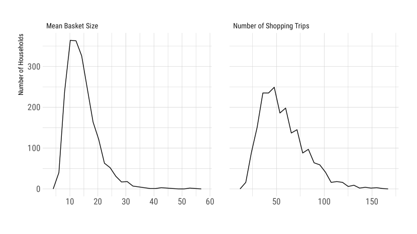
Figure 1: Household Summary Statistics: Tuesday and Wednesday Only

4.2 Models

4.2.1 Nested Factorization

Our primary model is the Nested Factorization model, as outlined in Section 3.2.1. The key hyperparameters of the model are the dimensionality of the latent factorizations of the user preferences and elasticities. Allowing for a higher dimensional factorization allows for more flexibility in the shopping patterns the model is able to fit, at the expense of slower estimation speeds and larger potential for overfitting the data. In order to choose the values for these hyperparameters, we follow the standard practice in the computer science literature of selecting based on performance on a “validation” subset of the data that is distinct from the subset used to train the models (and distinct from the “test” subset that is “held out” and not used until the final comparison between models). We discuss the model selection criteria in more depth in Section 6. We compare the performance of the Nested Factorization model against several alternative approaches described in the following sections.

4.2.2 Multinomial Logit

The simplest and most commonly used discrete choice model is the multinomial logit [Train, 2016], which has a long history in economics tracing back to Luce [1959] and McFadden [1974].

We focus on a baseline specification that controls for household demographics (gender, age, marital status, and income) and include the weekly mean category purchase rates as pseudo-fixed effects for each calendar week, which helps control for seasonal trends that shift the demand for the product category and which may be correlated with the product prices. We have also tried alternative specifications that add behavioral controls based on splitting the population into 20% buckets based on total spending in the store and a model without demographic controls, all of which had similar predictive performance. Because of its poor predictive performance across all of the measures we focus on in this paper, we have omitted the multinomial logit results from some of the results charts and tables, when the additional entries detract from clarity.

Homogeneous with Demographic Controls:

$$U_{ijt} =\alpha_{j}+\eta\log p_{jt}+\beta_{j}D_{i}+week_{t}+weekday_{t}+\epsilon_{ijt}$$

4.2.3 Mixed Logit

The mixed, or random coefficients, logit is one approach for increasing the flexibility of the multinomial logit. By allowing the coefficients of the model to vary across the population, the mixed logit allows for correlation in unobserved factors over time and for more flexible patterns of substitution between products. McFadden and Train [2000] show that any choice probabilities derived from random utility maximization can be approximated arbitrarily well by a appropriately chosen mixed logit model. As Steenburgh and Ainslie [2013] point out, the mixed logit still constrains demand at the individual level to satisfy IIA, so it “improves upon, but does not completely solve the problems of the homogeneous logit model.”

Mixed with Demographic Controls and Random Price:

$$U_{ijt} =\alpha_{j}+\eta_{i}\log p_{jt}+\beta_{j}D_{i}+week_{t}+weekday_{t}+\epsilon_{ijt}$$

Mixed with Random Intercept and Price:

$$U_{ijt} =\alpha_{ij}+\eta_{i}\log p_{jt}+week_{t}+weekday_{t}+\epsilon_{ijt}$$

With sufficiently flexible distributional assumptions for the random coefficients $\alpha_{ij}$, a mixed logit model could have a similar degree of flexibility as the latent factorization based approach that we use in the Nested Factorization model. However, scaling such an approach can be computationally challenging, especially when the number of products is large. We estimate mixed logit models using the Stata implementation from Hole [2007], which allows each of the product intercepts $\alpha_{ij}$ to be distributed across households as independent normal distributions.

4.2.4 Nested Logit

Another method for relaxing the homogeneous logit model to allow for more flexible patterns of substitution is the nested logit model. In the nested logit model, the decisions a user faces are partitioned into “nests.” One interpretation of the nested logit structure is that a user first chooses which nest to purchase from, and then which product to choose from within the nest. An alternative interpretation frames the nesting structure as capturing common shocks that lead to correlation among the choice probabilities of products in the same nest. Within each nest, the choices satisfy the IIA substitution pattern, but the substitution between products in different nests is able to vary more flexibly. We choose the same simple nesting structure as was used in the NF model. We put the outside good in its own nest, and the remaining products in each category in a single shared nest. An additional term called the nesting coefficient or inclusive value term controls how the decision of which nest to choose depends on the utilities of the items within the nest. This nesting coefficient is analogous to the $\gamma_{i}^{T}\lambda_{c}$ term in the Nested Factorization (equation 8) with the restriction that the value be homogeneous across households. Within the product nest, choice follows the same functional form as used in the homogeneous logit model with demographic controls. In essence, the Nested Factorization can be thought of as an extension to a nested logit that allows for rich heterogeneity in consumer preferences and price sensitivities by means of a latent factorization approach.

Nested with Demographics:

$$U_{ijt} =\alpha_{j}+\eta\log p_{jt}+\beta_{j}D_{i}+\epsilon_{ijt}$$

4.2.5 Discrete Choice Models with HPF Controls

One disadvantage of the Nested Factorization functional form relative to the HPF form used in Gopalan et al. [2013] is that it leads to substantially slower estimation of the approximate posterior. The choice of functional form and priors in the original HPF form allows for a closed form for the gradient of the variational Bayes objective function. With the Nested Factorization model, we have to perform stochastic gradient descent using a noisy estimate of the gradient. In practice this leads the model to require substantially more time and iterations before convergence.

This motivates an alternative approach that approximates the full Nested Factorization model with a two step approach. Estimate each shopper’s preferences over items using the HPF model. Then, take the estimated utility values for each shopper and item and plug these values in as covariates into standard discrete choice models. This “HPF controls” approach can be thought of as an approximation to the generally infeasible approach of having separate fixed effects for each household item pair (i.e. $N\times J$ separate parameters).

Hierarchical Poisson Factorization (HPF):

$$y_{ijt} \sim\text{Poisson}(\mu_{ij})$$

$$\mu_{ij} =\underbrace{\theta_{i}^{T}\beta_{j}}_{\text{Latent - Latent}}+\underbrace{W_{i}^{T}\rho_{j}}_{\text{User Observables}}+\underbrace{\sigma_{i}^{T}X_{j}}_{\text{Item Observables}}$$

This model predicts user $i$ will purchase item $j$ at a mean rate of $\mu_{ij}$, so we can analogize it to a discrete choice model within a category with utility taking the form $u_{ijt}=\log(\mu_{ijt})+\epsilon_{ijt}$, which will generate approximately the same choice probabilities for each item in the category $c$.

This two step procedure may also prove helpful in contexts where it is important to incorporate additional complications that are difficult to directly embed into the full NF Bayesian model. For example, it may be effective to include these HPF controls into models of dynamic discrete choice such as those that arise from storable goods [Hendel and Nevo, 2006] or from consumer learning [Ackerberg, 2003] as a simple way to allow richer heterogeneity in consumer preferences (at the cost of lower statistical efficiency and potentially bias from estimating as a two step procedure rather than simultaneously).

This approach may also add value by allowing researchers to take advantage of data that might otherwise go unused. Often researchers have access to a broader set of data than the sample they focus on for their primary analysis. This might be done in order to take advantage of a subset of the data which was affected by some source of quasi-experimental variation or may be due to other desirable properties of a particular subset of users or products. Latent factorization approaches, such as HPF, may be able to extract useful signal from the broader set of data, which can then be applied to improve the precision or flexibility of the primary analysis that focuses on a specific subsample of the data.

5 Identification and Placebo Tests

In our data, almost all price changes occur on Tuesday nights, near midnight, when very few customers are shopping. Thus, we can think of the price change as separating Tuesday and Wednesday. This motivates an empirical specification in which we use only the data from Tuesday and Wednesday in order to focus narrowly to the days immediately before and after price changes. We then include controls at the category level for each week and a indicator variable for Wednesday. The “identifying assumption” for learning price elasticities from this specification is that any differences in a particular consumer’s preferences for items between Tuesday and Wednesday are constant across weeks; in other words, weeks may differ from one another, but the Tuesday to Wednesday trend is constant over time. We also exclude the data from weeks immediately prior to major US Holidays out of a concern that this assumption is less likely to hold in these weeks e.g. the difference between the shopping patterns on the Tuesday and Wednesday before Thanksgiving may systematically differ from pattern that holds during more typical weeks. We find in our analysis that the Wednesday effect is small, with the average difference in category purchase probabilities between Tuesday and Wednesday of 0.127% (a 3.5% relative change in purchase probability).

In order to assess the validity of our assumptions, we present some supplementary analysis in the spirit of the literature on treatment effects [Athey and Imbens, 2017]. In particular, we test for the presence of certain types of price endogeneity by taking the price coefficients we get from the actual price data and comparing to the price coefficients we would get from a model fit on a data with the prices shifted forwards or backwards across time. We do this in two ways, first by shifting the price of a single UPC in each category (and giving that UPC a separate price coefficient), and second by simultaneously shifting the prices of all items in the category. To create the forward shifted price series for a product, we move each week with a price change forward to the first week that had no price changes in the real data. We repeat this process for each of the 123 product categories and plot the resulting distribution of price coefficients and p-values for the price coefficients. The desired result is that the shifted price series result in an approximately uniform distribution of p-values, since the artificial price changes should have no effect on consumer purchase behavior. The following results are based on the basic multinomial logit specification (with the pseudo week effects, which are calculated as the category level mean purchase rate in the week).

Out of the 123 categories, 13 fail one of the four placebo tests at the 1% level. If we only considered unconfoundedness checks that shift prices backwards, only 4 categories fail one of the two backward shifting tests. Backwards shifts would fail in the presence of consumers who are aware of future price changes. Forward shifts can fail for goods for which stockpiling is possible. Some of the categories that fail with the forward shifted price are durable/storable (e.g. Baking Mixes, Ketchup, and Bag Frozen Vegetables), but other categories seem more likely be failing for other reasons (e.g. Refrigerated Turkey and Tomatoes).

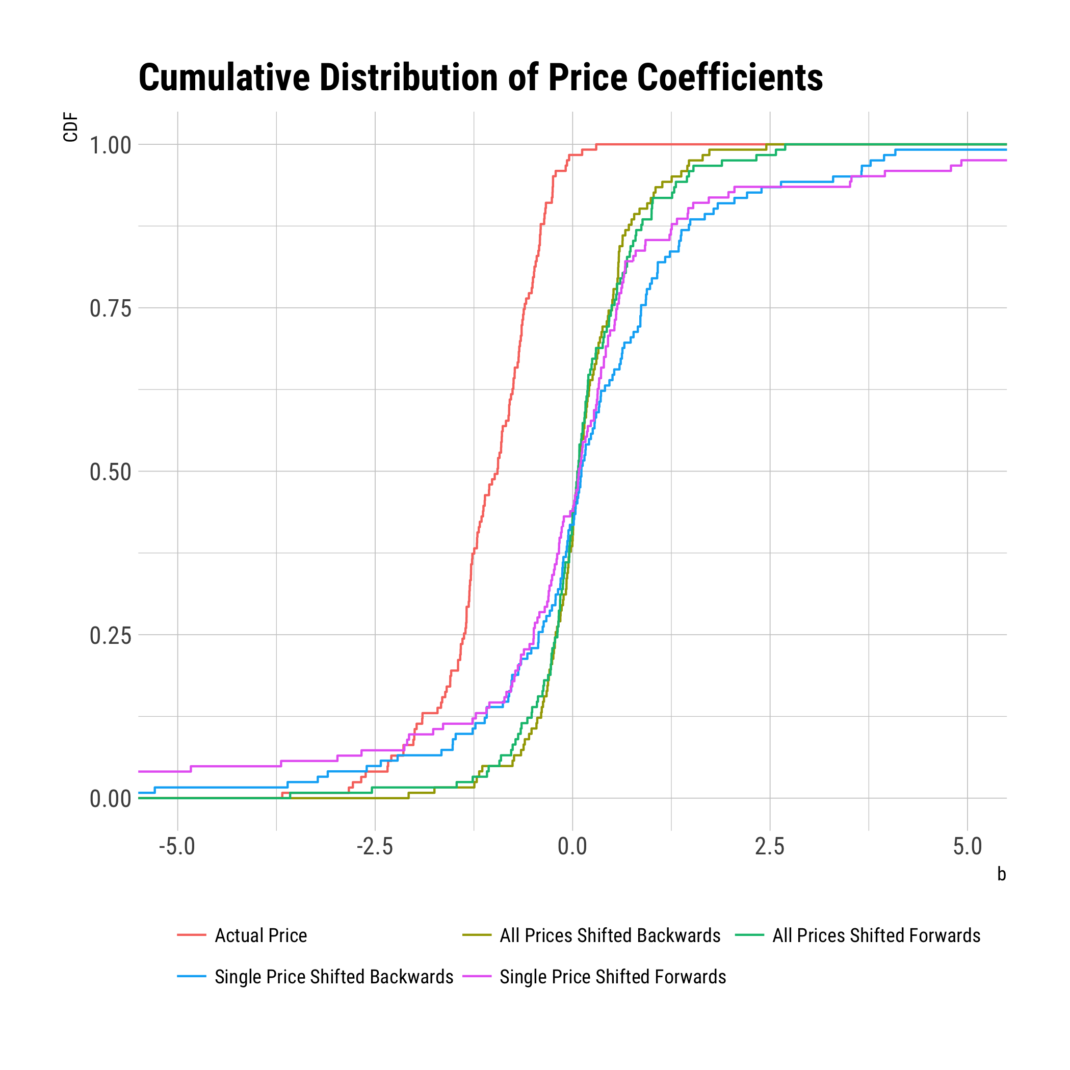
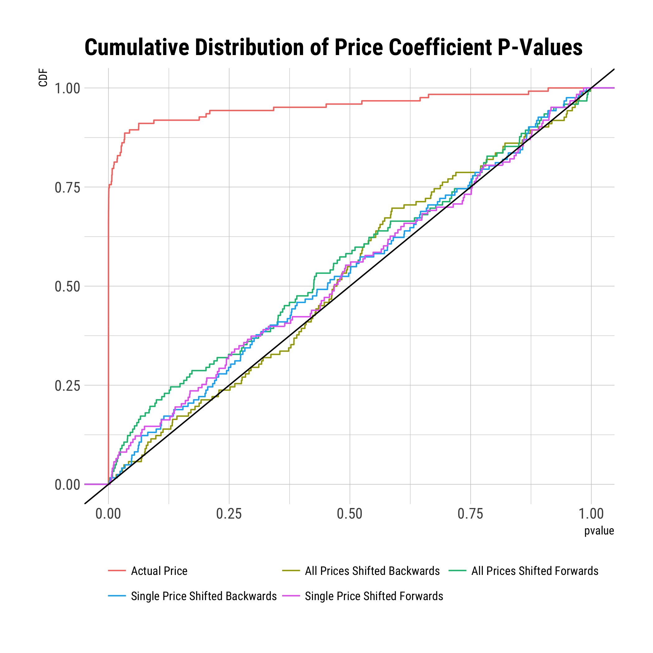
Figure 2: Comparison of price coefficients and p-values with actual price series vs. with prices shifted forwards or backwards

6 Assessing Model Performance and Fit

In the machine learning literature, it is typical to split data into three non-overlapping parts: a training set, a validation set, and a test set. The training data is used to fit the parameters of the model. To the extent the model has hyperparameters that must be set prior to estimation, the model estimation can be repeated under different values of the hyperparameters. The validation set is used to select a model (i.e. to make a choice of hyperparameters) based on each model’s predictive performance on the validation set. Finally, the predictive performance on held-out test data is used to evaluate the performance of the chosen model. Under the assumption that all observations are drawn from the same data generating process, then the predictive performance on the test set is an unbiased estimate of the model’s ability to make predictions on new data. In Section 6.1, we compare Nested Factorization and the set of alternative models in terms of their predictive fit on the held-out test sample of data.

However, this notion of predictive performance on held-out data does not evaluate the ability of a model to make causal predictions of what “would” happen if we took actions that changed the distribution of the data. For example, a model trained to predict the demand for hotel rooms, might correctly identify that hotels are often full when prices are high and have many empty rooms when prices are low. This, however, may be due to hotels setting prices in expectation of demand, rather than because consumers prefer to pay high prices. Such a model could be highly predictive of hotel demand based on a randomly selected held-out test set (which is drawn from data generated under the existing data generating process), however such a model would perform poorly at predicting what prices a hotel ought to charge (since changing prices will change the data generating process). It is concerns about such endogeneity of prices that motivates our identification approach that relies on focusing on data immediately before and after price changes (Tuesdays and Wednesdays), including weekly time controls (which can absorb any seasonal/holiday trends), including a indicator variable for Wednesdays (to absorb any consistent differences in Tuesday vs Wednesday demand), and excluding data from the weeks of major US Holidays. Since all models include the weekly controls at the category level, they all have the ability to predict average demand in a week at that level. However, in weeks with price changes, only a model that has accurately estimated consumer preferences about price can account for which day within the week is expected to have more purchases.

To validate the ability to make predictions about counterfactuals, we focus on three types of changes that can occur during a week for a particular product: (a) change in the price of the product (b) a change in the price of a different product in the same category and (c) another item in the category going into or out of stock. If the identifying assumptions of our models hold, then we can think of each of these events as a small sources of quasi-experimental variation. While the outcomes of each of these quasi-experiments is likely to be noisy, we can improve the precision of our estimates by averaging across a large number of them.

In Section 6.2, we compare the log likelihoods of the individual household level predictions during weeks in which one of these “counterfactuals” occurs in order to evaluate how well each model is able to make predictions that capture the change in predicted demand before and after the change (relative to the week-level average captured by the weekly time controls). In addition, we also compare the ability of each model to make predictions about the change in aggregate demand from Tuesday to Wednesday during weeks in which one of these events occurs. Our test set holds out data at the household-week level; this allows us to estimate overall consumer preferences and test our ability to predict household purchases on trips that were excluded from the training data, and in particular in weeks where the week-category effect estimated using other consumers’ purchases in that week is insufficient to predict the average probability of consumers purchasing on a particular day of the week (since prices differ across days). We use select hyperparameters (tune the model) using only validation set data from item-weeks with price changes, and we evaluate performance in the test set based on the three changes (a)-(c) outlined above.

In Section 6.3, we further evaluate the performance of our model at making predictions in scenarios of interest for counterfactual inference. We compare models in terms of their ability to capture heterogeneity in preferences across the population of households and evaluate the degree to which the predicted heterogeneity is predictive of actual behavior in the held-out test set. For example, we compare the predictions made for households who in the training data sample never purchased a particular UPC or have made no purchases at all from an entire product category. Among this group of “never buyers”, we show that the Nested Factorization model is able to correctly predict which of these households are relatively more or less likely to make a purchase in the held-out test data.

Section 6.4 examines the estimated own-price and cross-price elasticities. Finally, Section 6.5 looks at the potential for targeted marketing efforts that are personalized based on the rich heterogeneity estimated by the Nested Factorization model.

6.1 Predictive Fit

Table 1: Comparison of Predictive Fit

	Mean Log Likelihood		Mean Squared Error
Model	Train	Test	Train	Test
Nested Factorization	-4.2271	-4.9096	0.8981	0.9268
Mixed Logit with Random Price and HPF Controls	-4.9233	-5.3125	0.9473	0.9660
Nested Logit with HPF Controls	-5.2345	-5.4230	0.9583	0.9650
Multinomial Logit with HPF Controls	-5.2307	-5.4248	0.9583	0.9651
Mixed Logit with Random Price and Demographics	-5.2976	-5.5690	0.9780	0.9898
Mixed Logit with Random Price and Random Intercepts	-5.3956	-5.5827	0.9785	0.9849
Nested Logit with Demographic Controls	-5.6080	-5.6779	0.9788	0.9801
Multinomial Logit with Demographic Controls	-5.6142	-5.6791	0.9791	0.9803

In Table 1, we compare the predictive fits of each of the models. Comparing the overall predictive accuracy across all models, the Nested Factorization model has the highest likelihood and the lowest sum of squared errors among all models on both the training data and the held-out test sample. In addition, each of the models that include HPF controls perform better than the models that use control only for demographics.

6.1.1 Comparison of Predictive Fit by Category

We can also compare how each model performs relative to the NF model at the level of individual categories. In Table 2, we calculate the relative rank of each model’s performance in the test set separately for each category. The Nested Factorization model has the highest log likelihood in 86% of categories and the lowest squared error in 96%. This demonstrates the effectiveness of learning preferences simultaneously across many product categories. Even if we were only interested in understanding consumer preferences in one particular category, e.g. yogurt, it can be effective to train a model using the data from other categories as well, either using the full Nested Factorization model or by using the HPF controls, which also consistently improve predictive performance on the held-out test data in most categories.

Table 2: Comparison of Predictive Fit By Category

	Mean Rank		% Best Performance
Model	Log L	SE	Log L	SE
Nested Factorization	1.53	1.10	86.2%	95.9%
Mixed Logit with Random Price and HPF Controls	2.40	5.33	9.8%	0.8%
Nested Logit with HPF Controls	3.87	3.38	0.0%	0.8%
Multinomial Logit with HPF Controls	4.21	3.63	0.8%	0.8%
Mixed Logit with Random Price and Random Intercepts	4.69	5.65	0.8%	1.6%
Mixed Logit with Random Price and Demographics	5.21	7.07	2.4%	0.0%
Nested Logit with Demographic Controls	6.96	4.93	0.0%	0.0%
Multinomial Logit with Demographic Controls	7.13	4.91	0.0%	0.0%

Mean rank is calculated as the average across product categories of the rank ordering of models based on predictive fit, with rank 1 corresponding to the model with the lowest error.

6.1.2 Comparison of Fits by Household and UPC

To help understand where the improvement in predictive performance is coming from, we can spit the results by the popularity of the products or by the shopping frequency of the households. In Figure 4, we can see that all models are more accurate in their predictions for the more commonly purchased UPCs (percentile 100) than for the less common items. Across all percentiles, the Nested Factorization model does consistently better than the alternative models. The models that use HPF effects (solid lines) have much smaller, but consistent gains over the nested and mixed logit models that use demographic or behavioral controls. Similar trends can be seen when we divide the results based on the number of purchases each household made in the training data in Figure 4. This suggests the benefits from a latent-factorization-based approach are relatively uniform across households and products.

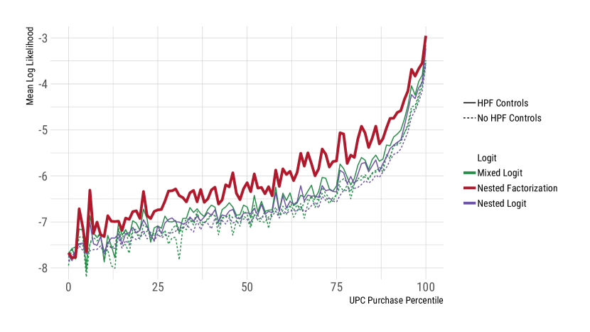
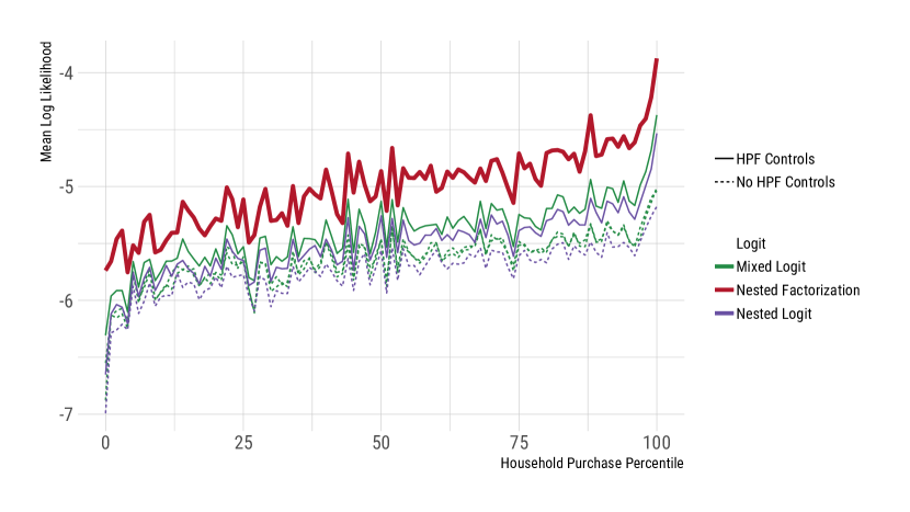
Figure 3: Test Set Predictive Fit by UPC Purchase Frequency

Figure 4: Test Set Predictive Fit by Household Purchase Frequency

6.2 Price Change and Availability Counterfactuals

In the economics and marketing literatures, models of consumer demand are used to make inferences about what would happen if change were made to a market. For example, such models have been used to predict what would happen if prices were changed, if products are added or removed from a market, or if competing firms in the market were to merge. As discussed in Section 6, evaluating the predictive fit of a model, even when done on a held-out test sample, does not reliably determine whether a model can be used to make predictions under counterfactual states of the world such as these. To evaluate the ability to make predictions under changes to prices or product availability, we focus on each model’s predictions on held-out test set data immediately before and after such changes occur. Under the assumption that these changes are exogenous conditional on our week and weekday controls, we can think of each of these changes as a miniature experiment. By pooling across many such small noisy experiments, we can increase our precision in detecting differences in performance. We focus on three types of changes that can occur between Tuesday and Wednesday for a particular UPC. First, we look at weeks in which the focal product’s price changes, which we can think of as evaluating the accuracy of the model’s own-price elasticity estimates. Second, we look at weeks in which some other product in the focal product’s category has a price change, in order to evaluate the predicted cross-price elasticities. Finally, we look at weeks in which some other product in the focal product’s category goes into or out of stock, which is another measure of the patterns of substitution between products. We asses fit on the test data using three measures. The first measure is the mean log likelihood of the individual household level predictions for product weeks that experienced the corresponding counterfactual event. The second and third measure compare the actual aggregate demand to the predicted aggregate demand across all households in the test set who shopped during the corresponding weeks. For products that are purchased at least 2.5 times on average per day, we calculate the likelihood of the Tuesday to Wednesday change in aggregate demand as approximated by a Skellam distribution. For less popular products, we calculate the likelihood of observing aggregate demand greater than zero, which we approximate with a Bernoulli distribution whose mean is the sum of the household level predictions.

Table 3: Mean Log Likelihood by Counterfactual Event

	Individual		Aggregate
Model	Popular	Less Common	Popular	Less Common
All Weeks
Nested Factorization	-0.1070 (0.0004)	-0.0173 (0.0001)	-2.5356 (0.0146)	-1.3072 (0.0044)
Mixed Logit with Random Price and HPF Controls	-0.1156 (0.0004)	-0.0188 (0.0001)	-2.5562 (0.0145)	-1.3365 (0.0037)
Nested Logit with HPF Controls	-0.1194 (0.0005)	-0.0191 (0.0001)	-2.5568 (0.0154)	-1.3105 (0.0040)
Multinomial Logit with HPF Controls	-0.1194 (0.0005)	-0.0191 (0.0001)	-2.5554 (0.0154)	-1.3086 (0.0040)
Mixed Logit with Random Price and Random Intercepts	-0.1263 (0.0005)	-0.0194 (0.0001)	-2.5712 (0.0146)	-1.3316 (0.0037)
Mixed Logit with Random Price and Demographics	-0.1240 (0.0004)	-0.0195 (0.0001)	-2.5934 (0.0153)	-1.3543 (0.0038)
Multinomial Logit with Demographic Controls	-0.1290 (0.0005)	-0.0197 (0.0001)	-2.5722 (0.0157)	-1.3105 (0.0040)
Nested Logit with Demographic Controls	-0.1289 (0.0005)	-0.0197 (0.0001)	-2.5740 (0.0157)	-1.3113 (0.0041)
Cross Price Weeks
Nested Factorization	-0.0925 (0.0008)	-0.0149 (0.0001)	-2.4527 (0.0262)	-1.2017 (0.0084)
Mixed Logit with Random Price and HPF Controls	-0.1006 (0.0008)	-0.0163 (0.0001)	-2.4846 (0.0258)	-1.2584 (0.0069)
Nested Logit with HPF Controls	-0.1041 (0.0009)	-0.0164 (0.0001)	-2.4844 (0.0277)	-1.2177 (0.0076)
Multinomial Logit with HPF Controls	-0.1041 (0.0009)	-0.0164 (0.0001)	-2.4836 (0.0276)	-1.2165 (0.0076)
Mixed Logit with Random Price and Random Intercepts	-0.1139 (0.0009)	-0.0168 (0.0001)	-2.5002 (0.0260)	-1.2527 (0.0069)
Mixed Logit with Random Price and Demographics	-0.1111 (0.0009)	-0.0170 (0.0001)	-2.5132 (0.0280)	-1.2752 (0.0071)
Multinomial Logit with Demographic Controls	-0.1162 (0.0010)	-0.0170 (0.0001)	-2.4966 (0.0279)	-1.2182 (0.0077)
Nested Logit with Demographic Controls	-0.1161 (0.0010)	-0.0170 (0.0001)	-2.5066 (0.0292)	-1.2194 (0.0078)
Own Price Weeks
Nested Factorization	-0.1374 (0.0009)	-0.0229 (0.0001)	-2.7871 (0.0360)	-1.5544 (0.0104)
Mixed Logit with Random Price and HPF Controls	-0.1465 (0.0009)	-0.0243 (0.0001)	-2.8004 (0.0357)	-1.5475 (0.0086)
Nested Logit with HPF Controls	-0.1493 (0.0009)	-0.0249 (0.0001)	-2.7986 (0.0371)	-1.5356 (0.0092)
Multinomial Logit with HPF Controls	-0.1493 (0.0009)	-0.0249 (0.0001)	-2.7949 (0.0373)	-1.5321 (0.0092)
Mixed Logit with Random Price and Random Intercepts	-0.1530 (0.0009)	-0.0251 (0.0001)	-2.8003 (0.0348)	-1.5408 (0.0085)
Mixed Logit with Random Price and Demographics	-0.1525 (0.0009)	-0.0251 (0.0001)	-2.8544 (0.0374)	-1.5709 (0.0090)
Multinomial Logit with Demographic Controls	-0.1557 (0.0010)	-0.0256 (0.0002)	-2.8097 (0.0369)	-1.5344 (0.0092)
Nested Logit with Demographic Controls	-0.1555 (0.0010)	-0.0256 (0.0002)	-2.8186 (0.0372)	-1.5377 (0.0093)
Out of Stock Weeks
Nested Factorization	-0.0924 (0.0040)	-0.0159 (0.0002)	-2.3349 (0.1114)	-1.2746 (0.0129)
Mixed Logit with Random Price and HPF Controls	-0.1033 (0.0044)	-0.0173 (0.0002)	-2.3679 (0.1225)	-1.3064 (0.0111)
Nested Logit with HPF Controls	-0.1068 (0.0046)	-0.0176 (0.0002)	-2.3427 (0.1243)	-1.2817 (0.0122)
Multinomial Logit with HPF Controls	-0.1068 (0.0046)	-0.0176 (0.0002)	-2.3446 (0.1259)	-1.2774 (0.0121)
Mixed Logit with Random Price and Demographics	-0.1091 (0.0045)	-0.0180 (0.0002)	-2.3669 (0.1132)	-1.3249 (0.0118)
Mixed Logit with Random Price and Random Intercepts	-0.1125 (0.0046)	-0.0181 (0.0002)	-2.3403 (0.1156)	-1.3068 (0.0113)
Multinomial Logit with Demographic Controls	-0.1146 (0.0048)	-0.0183 (0.0002)	-2.3261 (0.1189)	-1.2800 (0.0122)
Nested Logit with Demographic Controls	-0.1145 (0.0047)	-0.0183 (0.0002)	-2.2974 (0.0990)	-1.2840 (0.0123)

6.3 Comparison of Degree of Personalization across Households

To examine the extent to which each of these models is able to flexibly model the differences in preferences between households, we calculate two measures of the degree of “personalization” of the predicted purchase rates that each model predicts for each household. First, we compare the coefficient of variation of a models predictions at the UPC level and the category level. As a second measure, we regress the predicted purchase rate on the actual purchase rate in the in the held-out test sample.

Table 4 shows that the Nested Factorization model has the largest variation in the predictions across households and that this variation is strongly correlated with variation in the actual purchase rates in the held-out test data. For each $1\%$ increase in the Nested Factorization model’s prediction of a household’s purchase for a UPC, the household’s actual purchase rate in the test set increases by $0.9955\%$.

Table 4: Comparison of Degree of Personalization of Predictions across Models

	Coef. of Variation		Regression Coef.
Model	UPC	Category	UPC	Category
Nested Factorization	3.2546	1.7756	0.9955	1.0023
Mixed Logit with Random Price and HPF Controls	2.0747	1.6085	0.6861	0.7007
Mixed Logit with Random Price and Demographics	1.3869	1.5724	0.4718	0.5968
Multinomial Logit with HPF Controls	1.2590	0.7276	0.8402	0.8893
Nested Logit with HPF Controls	1.2368	0.7520	0.8417	0.8725
Mixed Logit with Random Price and Random Intercepts	1.0834	1.0446	0.4666	0.6959
Nested Logit with Demographic Controls	0.4465	0.2967	0.8947	0.9314
Multinomial Logit with Demographic Controls	0.4337	0.2756	0.9077	0.9411

6.3.1 Predicting Preference for Products a Household has Not Yet Purchased

The Nested Factorization model is also able to make predictions about the strength of a households preferences for a given UPC, even if the household has never purchased that particular item before. To demonstrate this, we look at the set of all households who have made 0 purchases of a particular UPC in the training sample. For each UPC and each predictive model, we can rank these households based on their predicted purchase rate and group them into deciles. We carry out a similar analysis of households who made no purchases from an entire product category during the training sample. Figure 5 shows that the Nested Factorization model is able to correctly predict which households are relatively more or less likely to purchase a category or UPC that they never purchased during the training sample. The decile of households with the highest predicted likelihood to purchase a product category for the first time, purchases at roughly 3 times the frequency of the lowest decile. At the UPC level, this ratio of purchase rates in the held-out test sample is more than 10 fold difference. The models with HPF controls (solid lines) are able to capture a smaller amount of this variation The models without either approach for latent factorization (dotted lines) have substantially less predictive power for these first time buyers. This may be useful to applied marketing practitioners who may be interested in targeting advertising or promotions towards new customers who might be interested in a product that they have not yet tried.

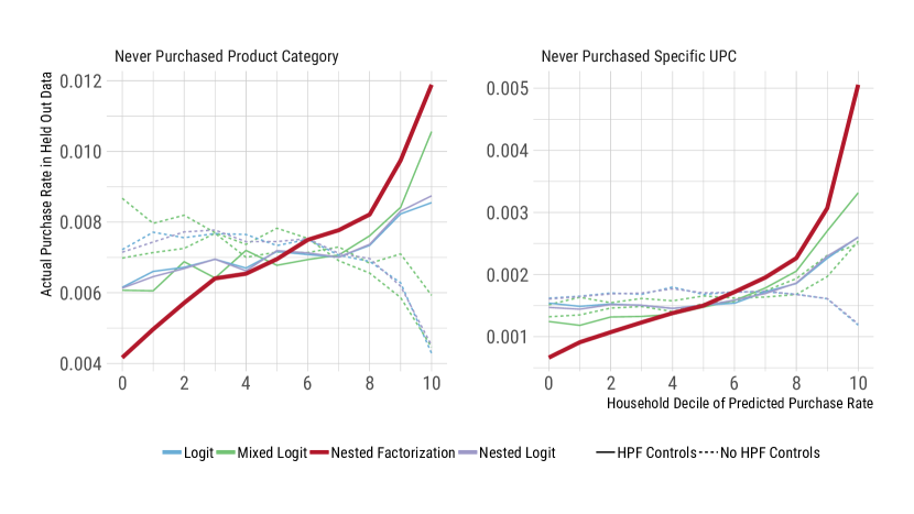
Figure 5: True purchase rate in held out test set for households who never purchased the UPC/Category in the training sample.

6.4 Estimated Elasticities

6.4.1 Cross-Price Elasticities Within and Between Products Subcategories

A different approach for assessing models is to see how well each does at learning patterns that we believe to be true about the world. None of the models were given data from the product hierarchy data about the “class” or “subclass” each product is categorized under. These groupings are more fine grained than the “category” level that we focused on for modeling product substitution. Nevertheless, we show that the Nested Factorization model correctly infers that products that are in the same class or subclass are more similar to each other, and as a result these models predict higher levels of cross-price elasticities between products that are in the same class or subclass than between items that are in different classes/subclasses.

Table 5: Comparison of Cross-Price Elasticities

	Class Cross Price			Subclass Cross Price
Model	Inside	Outside	%	Inside	Outside	%
Nested Factorization	0.0186	0.0080	132%	0.0196	0.0181	8.4%
Nested Logit with Demographic Controls	0.0119	0.0086	37%	0.0125	0.0115	8.5%
Mixed Logit with Random Price and Random Intercepts	0.0062	0.0053	16%	0.0062	0.0062	-0.7%
Mixed Logit with Random Price and HPF Controls	0.0063	0.0054	16%	0.0063	0.0065	-3.9%
Multinomial Logit with HPF Controls	0.0035	0.0030	16%	0.0036	0.0035	0.8%
Multinomial Logit with Demographic Controls	0.0034	0.0029	16%	0.0034	0.0034	2.1%
Mixed Logit with Random Price and Demographics	0.0067	0.0060	13%	0.0066	0.0069	-4.6%
Nested Logit with HPF Controls	0.0148	0.0158	-7%	0.0140	0.0157	-10.7%

We compare the mean estimated elasticities for products that are/aren’t in the same product class or product subclass. We would expect the cross-price elasticities inside of a class or subclass to be higher than those outside the class, since this implies substitution towards products that are more similar.

6.4.2 Aggregate Demand Curves

In Figure 6, we validate whether the households with higher predicted elasticities do in fact respond more to price changes in held-out test data. To do this, for each UPC we split households into terciles based on their predicted elasticity. We then compare the Tuesday-Wednesday change in aggregate demand in the test set depending on the size of the price change during the week. The household’s with the higher predicted elasticities do in fact appear to have aggregate demand that is more responsive to price changes. This establishes that the heterogeneity we estimate is useful for counterfactual predictions about heterogeneity in consumer response to price changes.

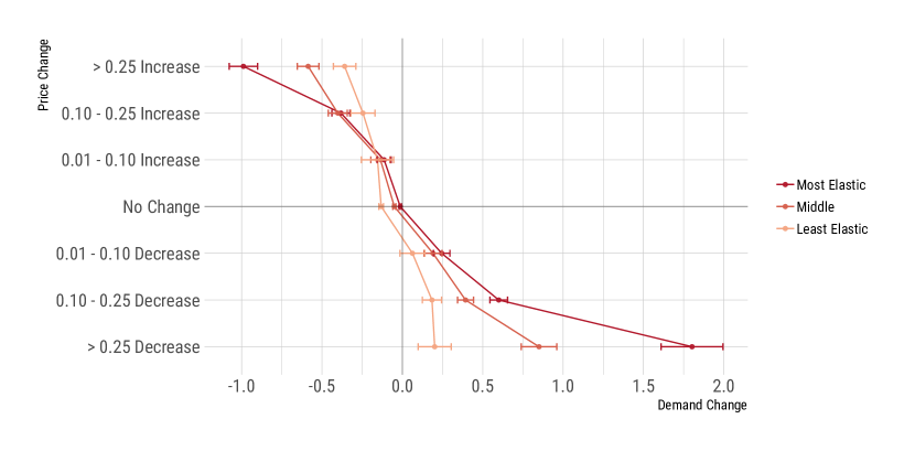
Figure 6: Test Set Aggregate Demand Change by Elasticity Tercile

6.5 Target Marketing

Understanding how preferences vary across customers can serve as an important input into the decision of how to allocate resources across marketing efforts such as advertising and coupons. In Table 6, we carry out an analysis similar to the classic study by Rossi et al. [1996] to estimate the potential impact of targeting coupons to customers based on their purchase histories. For each product category, we use each model to select the 30% of households for whom it would be most profitable for the store to offer a 30% off coupon for the most popular UPC in the category. We then evaluate how profitable this coupon targeting would be using the Nested Factorization model as ground truth. For each model, we evaluate three approaches to targeting the coupons. Under individualized targeting, the store is able to select individual households when choosing whom to target with the coupons. Under demographic targeting, the coupons must be allocated in a way that is uniform within demographic groups. Under behavioral targeting, the coupons must be allocated based on the number of times a household has made purchases in the product category. Under each scenario, we compare the predicted store profits to the profits that would have been earned if the store had allocated the coupons uniformly at random.

Table 6: Gains from Targeted Discounts:

	% Gains Relative to Uniform
Model	Behavioral	Demographic	Individualized
Nested Factorization (linear)	2.57%	4.55%	28.5%
Mixed Logit with Random Price Effects and HPF Controls (linear)	1.51%	2.38%	5.7%
Multinomial Logit with HPF Controls (linear)	1.37%	1.60%	5.7%
Nested Logit with HPF Controls (linear)	1.41%	1.57%	5.4%
Nested Logit with Demographic Controls (linear)	0.56%	3.03%	4.7%
Multinomial Logit with Demographic Controls (linear)	0.77%	2.17%	3.4%
Mixed Logit with Random Price Effects and Demographics (linear)	0.75%	2.53%	3.1%
Mixed Logit with Random Price and Random Intercepts (linear)	0.86%	1.31%	2.5%

Unfortunately, without the ability to run an experiment, it is difficult to validate our model’s predictions of the household specific profitability of pricing decisions. We can however approximate such an experiment by looking at consumers’ purchasing behavior under the various price regimes that happened to have occurred during each consumer’s test sample shopping trips. For each UPC, we identify the two most common prices, and for each consumer use our model to predict which of the prices will lead to higher store profits. We can then compare the average profit per shopping trip from the focal UPC under the two chosen prices. We aggregate these profits across the two groupings of households and calculate the increase in average profits per shopping trip from households shopping at their targeted price relative to the other price. In Figure 7, we can see that on average the store earns substantially more profit from households when they shop on days with the price that we predicted would lead to higher profits.

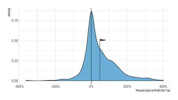
Figure 7: Distribution of Gain in Profit from Targeted Price
Percent gain calculated as $\frac{\text{Difference in Average Profit}}{\text{Average Profit}}$ for each item and price group, where the difference in average profit is the mean profit per shopping trip under the preferred price minus the mean profit per shopping trip under the alternative price.

In principal, a similar approach could be used to evaluate a model’s predictions about which users are most likely to switch brands when a new product enters a category. Unfortunately in our application, the sample selection criteria we used dropped most products that entered or exited the market during the sample period.

7 Conclusion

This paper proposes the Nested Factorization model for learning consumer preferences from panel data. This model allows rich heterogeneity in preferences and price responsiveness across consumers, and it gains efficiency and precision from simultaneously learning consumer preferences across many product categories. Using recent advances in variational Bayesian inference with stochastic gradient descent allows the model to remain tractable on the types of relatively large data sets that are increasingly becoming available as digitization progresses. We show that this approach can yield substantial improvements in out of sample predictive accuracy. This model is also able to predict price elasticities and patterns of substitution between products, which are often ignored or explicitly assumed away in most of the related recommender systems literature from computer science. Using the nested functional form, inspired by the nested logit model, allows our model to more efficiently learn these patterns of cross product substitution. We demonstrate an approach for validating a model’s ability to make predictions for counterfactual questions, by leveraging the large number of price changes and changes in product availability that occur in the data. Treating each such change as a “mini experiment”, we can evaluate a model’s predictions before and after the change on held-out data that was not used to fit the model. Pooling across many such sources of variation in the data reduces the noise and allows us to compare models in terms of their ability to make counterfactual predictions. We evaluate the potential gains from using flexible personalized models such as the one we propose here for targeting marketing efforts such as personalized price discounts or for identifying new consumers who might be interested in trying a product. More generally, we believe that flexible models of consumer demand, such as the Nested Factorization model proposed here, can be a useful tool for guiding the marketing strategies of firms or as part of a larger model for understanding patterns of competition between firms.

Declarations and Acknowledgments

• Acknowledgments: We are grateful to Tilman Drerup and Ayush Kanodia for exceptional research assistance. We thank the seminar participants at Harvard Business School, Stanford, the Microsoft Digital Economy Conference, and the Munich Lectures.

• Funding: We acknowledge generous financial support from Microsoft Corporation, the Sloan Foundation, the Cyber Initiative at Stanford, and the Office of Naval Research grant N00014-17-1-2131. Robert Donnelly is currently employed at Instacart (San Francisco, USA) but contributed to this research while a graduate student at Stanford Graduate School of Business. Ruiz is currently affiliated with DeepMind (London, UK) but contributed to this research while at Columbia University (New York, USA) and the University of Cambridge (London, UK), supported by the EU H2020 programme (Marie Skłodowska-Curie grant agreement 706760). The views expressed herein do not necessarily represent the views of Instacart or DeepMind.

• Availability of data and materials: The dataset is available to researchers at Stanford and Berkeley by application; it has been used previously in other research papers (see https://are.berkeley.edu/SGDC).

• Code availability: https://www.github.com/rodonn/nested-factorization Additional implementations of related variational inference models are available at https://github.com/franrruiz/shopper-src and https://www.openicpsr.org/openicpsr/project/114442/version/V1/view

8 Appendix

8.1 Data Construction and Sample Selection

The filters we use to select categories for study are outlined as follows:

1. For many of the mixed and nested logit specifications, we encountered difficulty with convergence in some of the product categories. To reduce these issues we ran all of the logit specifications using the top 10 items in each category along with an eleventh “pooled” option that combined all of the less popular items in the category. The NF and HPF models were run without any pooling of items. To make for a fair comparison, we evaluate model fit using only the top 10 items in each category. The relative performance of the NF model improves further if we compare the sum of the predicted purchase probabilities for the pooled items to the pooled item prediction from the logit models.

2. We eliminate categories in which more than 15% of shopping trips contain multiple items from the category or more than 10% of trips contain multiple top 10 items. Since for these categories the assumption of unit demand was substantially violated. For any remaining shopping trips in which multiple items from the same category were purchased, we selected one item at random from among the purchased items (and treated the remaining items as unpurchased).

3. We eliminate categories where the average absolute within-category correlation of the top 10 items’ prices is greater than $0.75\%$. This address the challenge of identifying cross-price elasticities in a handful of categories in which virtually all prices move in parallel.

4. We only include categories where at least 2 of the top 10 items have price variation from Tuesday to Wednesday in one of the sample weeks and at least 1 of them top 10 UPCs has price changes of at least 10 cents in a least 10% of the sample weeks.

5. We eliminate the top 15% of categories with the strongest demand seasonality. For each UPC, we first calculate seasonality as the Herfindahl index of daily demands over the sample period. We then calculate the percentile of each UPCs Herfindahl index over all UPCs and define a category’s seasonality as the average of the category’s top 10 items’ percentiles. While our approach of category level time controls at the week level should be able to control for any category level seasonality, it is not able to control for seasonal trends that affect individual UPCs.

The pricing information in our data comes from the transactions, which means we need to infer the prices a customer would have paid for any items they did not purchase. In addition, we need to account for coupons and deals (e.g. buy 2 get 1 free) that may cause different customers shopping on the same day to pay different price per unit. To resolve this, we use the daily median transacted price per unit calculated. In the event of a day with zero purchases, we carry forward the price data from the previous day.

Our data on product availability (i.e. out-of-stock items) is at granular level as described Che et al. [2012] based on the times employees scan items as out of stock and when they are restocked. However, for simplicity all of the models are run at a daily level. We consider an item unavailable to all shoppers on any days in which it is listed as out-of-stock during more than 75% of shopping trips on that day.

8.2 Variational Inference Algorithm

In this section, we provide additional details on the implementation of the variational inference model that is used to estimate the Nested Factorization model.

Recall from Section 3.2.4 that for the product choice stage of the model, we would like to approximate the posterior distribution of the latent parameters $\ell_{p}=\{\theta_{i},\beta_{j},\rho_{j},\sigma_{i},\gamma_{i},\lambda_{j}\}$. For notational convenience we will rewrite this as $\ell=\{\ell_{1},\ldots,\ell_{K}\}$ where the number of latent parameters $K=3N+3J$, where $N$ is the number of households and $J$ is the number of products. We will approximate the posterior using a multivariate Gaussian distribution with a diagonal covariance matrix. In general, imposing this “mean-field” assumption may limit the ability of our variational distribution to approximate the exact posterior, however this structure often works quite well in practice and still allows substantial flexibility in the resulting posterior approximation.

$$q\left(\ell;\nu\right)=\mathcal{N}(\ell;\mu,\Sigma)=\prod_{k=1}^{K}\mathcal{N}(\ell_{k};\mu_{k},\sigma^{2}_{k})$$ (11)

We want to find the variational parameters $\nu=\{\mu_{1},\ldots,\mu_{K},\ldots,\sigma^{2}_{K}\}$ that minimize the KL divergence between the variational distribution $q\left(\ell;\nu\right)$ and the exact posterior $p(\ell\mid\bm{y},\bm{x})$.

$$q^{*}(\ell;\nu)=\operatorname*{arg\,min}_{\nu}KL\left(q(\ell;\nu)\mid\mid p(\ell\mid\bm{y},\bm{x})\right)$$ (12)

This can be rearranged to show that minimizing the KL divergence is equivalent to maximizing an expression known as the evidence lower bound (ELBO) [Blei et al., 2017].

$$\mathscr{L}(\nu) =E_{q(\ell;\nu)}\left[\log p(\bm{y}\mid\bm{x},\ell)-\log q(\ell;\nu)\right]$$

$$=E_{q(\ell;\nu)}\left[\sum_{t}\log p(\bm{y}_{t}\mid x_{t},\ell)+\log p(\ell)+\log q(\ell;\nu)\right]$$ (13)

Unfortunately, the expectation in Equation 13 is analytically intractable. However, we can still seek the value of $\nu$ that maximizes $\mathscr{L}(\nu)$ with stochastic gradient descent if we are able to find a tractable expression for an unbiased estimate of the gradient $\nabla_{\nu}\mathscr{L}(\nu)$. We can do this by applying an approach that is known as the reparametrization trick [Kingma and Welling, 2014, Titsias and Lázaro-Gredilla, 2014, Rezende et al., 2014].

To do this, we introduce a transformation of the latent variables, so that rather than directly drawing from the distribution $\ell\sim q\left(\ell;\nu\right)$, we instead draw a new auxiliary random variable $\varepsilon\sim\mathcal{N}(0,I_{K})$ from a standard multivariate Gaussian distribution. By applying the transformation $\mathcal{T}(\varepsilon;\nu)=\mu+\Sigma^{\frac{1}{2}}\varepsilon$ we can generate draws $\ell=\mathcal{T}(\varepsilon;\nu)$ such that $\ell\sim q(\ell;\nu)$.

For notational ease, we will denote the expression inside the expectation in Equation 13 as $f(\ell;\nu)$. We can now rewrite the expectation in the gradient of the ELBO as

$$\nabla_{\nu}\mathscr{L}(\nu)=\nabla_{\nu}E_{q(\ell;\nu)}\left[f(\ell;\nu)\right]=\nabla_{\nu}E_{\varepsilon}\left[f(\mathcal{T}(\varepsilon;\nu);\nu)\right]$$ (14)

Now, bringing the gradient inside of the expectation and applying the chain rule gives us

$$\nabla_{\nu}\mathscr{L}(\nu)=E_{\varepsilon}\left[\nabla_{\ell}f(\ell;\nu);\nu)\mid_{\ell=\mathcal{T}(\varepsilon;\nu)}\nabla_{\nu}\mathcal{T}(\varepsilon;\nu)\right]$$ (15)

To obtain this expression, we used the fact that $E_{\varepsilon}\left[\nabla_{\nu}f(\ell,\nu)\mid_{\ell=\mathcal{T}(\varepsilon;\nu)}\right]=0$, since the only dependence of $f(\ell;\nu)$ on $\nu$ is through the term $\log q(\ell;\nu)$ and the expected value of the score function is 0.

Now we can obtain a Monte Carlo estimate of the gradient of the ELBO by sampling values of $\varepsilon$ from the standard multivariate Gaussian in order to approximate this expectation. In addition to making draws of $\varepsilon$ to evaluate the expectation, we also subsample customer shopping trips in each iteration. This allows the estimation to more easily scale to large datasets. By scaling the gradient estimates to account for this sampling, we can maintain the unbiasedness of the gradient estimator.

8.2.1 Hyperparameters

For each of the variational parameters we use a prior variance of 1.0 and a prior mean of 0 and a batch size of 5000 (number of customer trips to sample in each step of the stochastic gradient descent). We do a hyperparameter grid search across:

• {20,40,80} for the dimension of the latent factorization $\theta_{i}\beta_{j}$

• {20,40,80} for the dimension of the price term $\gamma_{i}\lambda_{j}$

• With and without user demographics $W_{i}$

• With and without product characteristics $X_{j}$

• {0.001,0.005,0.01} learning rates (i.e. step size for gradient descent)

• Product level model only: whether price should enter linearly or in logs

• Category level model only: {10,20} for the dimension of the time factorization $\mu_{c}\delta_{t}$

We selected models based on counterfactual price performance on the validation set. The selected product level model has hyperparameters {80, 20, yes, no, 0.005, linear price}. The selected category level model has hyperparameters {40, 40, no, no, 0.01, 10}.

8.3 Estimated Elasticities and Purchase Probabilities

In this section we compare the predicted own price elasticities across models and how those predicted elasticities vary within and between products. Table 7 shows the median own price elasticity estimated by each model. SD(Mean) is the standard deviation across the mean product level own-price elasticities. This captures how much variability there is in elasticities across products. Mean(SD) is the mean of the standard deviation of elasticities across consumers within a specific product. This captures the amount of variability in elasticities across consumers for the same product.

Figures 9 and 8 show the predicted elasticities and purchase rates for a sample of products and categories (entries are hidden when their text box would overlap with another entry).

Table 7: Comparison of Own-Price Elasticities

Model	Median	SD(Mean)	Mean(SD)
Nested Factorization	-1.7121	1.2008	1.7774
Nested Logit with Demographic Controls	-1.2976	1.0377	0.0532
Mixed Logit with Random Price and Random Intercepts	-2.2024	1.7822	0.8387
Mixed Logit with Random Price and HPF Controls	-2.7077	1.9084	1.1294
Multinomial Logit with HPF Controls	-1.1841	0.8904	0.0060
Multinomial Logit with Demographic Controls	-1.1813	0.8837	0.0017
Mixed Logit with Random Price and Demographics	-3.0897	2.4546	1.4785
Nested Logit with HPF Controls	-1.1017	0.8783	0.0182

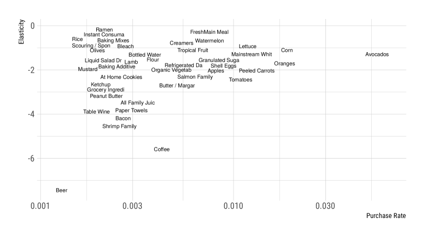
Figure 8: Category Level Elasticities and Predicted Purchase Probabilities:

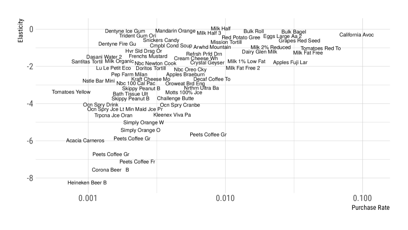
Figure 9: UPC Level Elasticities and Predicted Purchase Probabilities:

References

- Ackerberg [2001] D. Ackerberg. Empirically Distinguishing Informative and Prestige Effects of Advertising. The RAND Journal of Economics, 32(2):316–333, 2001. ISSN 0741-6261. doi: 10.2307/2696412. URL http://www.jstor.org/stable/2696412.
- Ackerberg [2003] D. Ackerberg. Advertising, Learning, and Consumer Choice in Experience Good Markets: An Empirical Examination. International Economic Review, 44(3):1007–1040, 2003. ISSN 0020-6598. URL http://www.jstor.org/stable/3663546.
- Athey and Imbens [2007] S. Athey and G. W. Imbens. Discrete choice models with multiple unobserved choice characteristics. International Economic Review, 48(4):1159–1192, nov 2007. ISSN 00206598. doi: 10.1111/j.1468-2354.2007.00458.x. URL http://onlinelibrary.wiley.com/doi/10.1111/j.1468-2354.2007.00458.x/abstract.
- Athey and Imbens [2017] S. Athey and G. W. Imbens. The State of Applied Econometrics - Causality and Policy Evaluation. Journal of Economic Perspectives, 31(2):3–32, may 2017. ISSN 0895-3309. doi: 10.1257/jep.31.2.3. URL http://pubs.aeaweb.org/doi/10.1257/jep.31.2.3.
- Athey and Stern [1998] S. Athey and S. Stern. An Empirical Framework for Testing Theories About Complementarities in Organizational Design. NBER Working Paper, 6600:1–38, 1998. doi: 10.1080/135943297399097. URL http://scholar.harvard.edu/files/athey/files/testcomp0498.pdf.
- Athey et al. [2018] S. Athey, D. Blei, R. Donnelly, F. Ruiz, and T. Schmidt. Estimating heterogeneous consumer preferences for restaurants and travel time using mobile location data. AEA Papers and Proceedings, 108:64–67, 2018. doi: 10.1257/pandp.20181031. URL http://www.aeaweb.org/articles?id=10.1257/pandp.20181031.
- Bai [2009] J. Bai. Panel Data Models With Interactive Fixed Effects. Econometrica, 77(4):1229–1279, 2009. ISSN 0012-9682. doi: 10.3982/ECTA6135. URL http://doi.wiley.com/10.3982/ECTA6135.
- Berry et al. [1995] S. Berry, J. Levinsohn, and A. Pakes. Automobile Prices in Market Equilibrium. Econometrica, 63(4):841, jul 1995. ISSN 00129682. doi: 10.2307/2171802. URL http://www.jstor.org/stable/2171802.
- Berry et al. [2004] S. Berry, J. Levinsohn, and A. Pakes. Differentiated Products Demand Systems from a Combination of Micro and Macro Data: The New Car Market. Journal of Political Economy, 112(1):68–105, nov 2004. ISSN 0022-3808. doi: 10.1086/379939. URL http://www.journals.uchicago.edu/doi/10.1086/379939.
- Berry et al. [2014] S. Berry, A. Khwaja, V. Kumar, A. Musalem, K. Wilbur, G. Allenby, B. Anand, P. Chintagunta, W. Hanemann, P. Jeziorski, and A. Mele. Structural models of complementary choices. Marketing Letters, 25(3):245–256, Aug. 2014. ISSN 0923-0645. doi: 10.1007/s11002-014-9309-y.
- Blei et al. [2017] D. M. Blei, A. Kucukelbir, and J. D. McAuliffe. Variational inference: A review for statisticians. Journal of the American Statistical Association, 112(518):859–877, 2017. doi: 10.1080/01621459.2017.1285773. URL https://doi.org/10.1080/01621459.2017.1285773.
- Bobadilla et al. [2013] J. Bobadilla, F. Ortega, A. Hernando, and A. Gutirrez. Recommender systems survey. Knowledge-Based Systems, 46:109–132, jul 2013. ISSN 09507051. doi: 10.1016/j.knosys.2013.03.012. URL http://linkinghub.elsevier.com/retrieve/pii/S0950705113001044.
- Che et al. [2012] H. Che, X. J. Chen, and Y. Chen. Investigating Effects of Out-of-Stock on Consumer Stockkeeping Unit Choice. Journal of Marketing Research (JMR), 49(4):502–513, aug 2012. doi: 10.1509/jmr.09.0528. URL http://journals.ama.org/doi/abs/10.1509/jmr.09.0528.
- Chintagunta [1994] P. K. Chintagunta. Heterogeneous logit model implications for brand positioning. Journal of Marketing Research, 31(May):304–311, 1994. doi: 10.2307/3152201. URL http://www.jstor.org/stable/3152201.
- Domencich and McFadden [1975] T. Domencich and D. McFadden. Urban Travel Demand: A Behavioral Analysis. North-Holland Publishing Co, 1975. ISBN 0444108300. URL https://trid.trb.org/view.aspx?id=48594.
- Dubé [2004] J.-P. Dubé. Multiple discreteness and product differentiation: Demand for carbonated soft drinks. Marketing Science, 2004. URL http://pubsonline.informs.org/doi/abs/10.1287/mksc.1030.0041.
- Dudik et al. [2011] M. Dudik, J. Langford, and L. Li. Doubly Robust Policy Evaluation and Learning. arXiv:1103.4601 [cs, stat], May 2011. URL http://arxiv.org/abs/1103.4601. arXiv: 1103.4601.
- Elrod [1988a] T. Elrod. Choice Map: Inferring a Product-Market Map from Panel Data. Marketing Science, 7(1):21–40, feb 1988a. ISSN 0732-2399. doi: 10.1287/mksc.7.1.21. URL http://pubsonline.informs.org/doi/abs/10.1287/mksc.7.1.21.
- Elrod [1988b] T. Elrod. Inferring an Ideal-Point Product-Market Map from Consumer Panel Data. Data, Expert Knowledge and Decisions, pages 240–249, 1988b. doi: 10.1007/978-3-642-73489-2˙20. URL http://www.springerlink.com/index/10.1007/978-3-642-73489-2_20.
- Elrod and Keane [1995] T. Elrod and M. P. Keane. A factor-analytic probit model for representing the market structure in panel data. Journal of Marketing Research, 1995. URL http://www.jstor.org/stable/3152106.
- Erdem et al. [2003] T. Erdem, S. Imai, and M. P. Keane. Brand and Quantity Choice Dynamics Under Price Uncertainty. Quantitative Marketing and Economics, 1(1):5–64, mar 2003. ISSN 1570-7156, 1573-711X. doi: 10.1023/A:1023536326497. URL http://link.springer.com/article/10.1023/A{%}3A1023536326497.
- Goettler and Shachar [2001] R. L. Goettler and R. Shachar. Spatial Competition in the Network Television Industry. Rand Journal of Economics, 32(4):624–656, 2001. ISSN 0741-6261. doi: 10.2307/2696385. URL http://goettler.simon.rochester.edu/research/papers/RAND_Winter2001_Goettler_Shachar.pdf.
- Gopalan et al. [2013] P. Gopalan, J. M. Hofman, and D. M. Blei. Scalable Recommendation with Poisson Factorization. arXiv:1311.1704 [cs, stat], nov 2013. URL http://arxiv.org/abs/1311.1704.
- Hausman and Wise [1978] J. A. Hausman and D. A. Wise. A Conditional Probit Model for Qualitative Choice: Discrete Decisions Recognizing Interdependence and Heterogeneous Preferences. Econometrica, 46(2):403, 1978. ISSN 00129682. doi: 10.2307/1913909. URL http://www.jstor.org/stable/1913909.
- Hendel [1999] I. Hendel. Estimating Multiple-Discrete Choice Models: An Application to Computerization Returns. Review of Economic Studies, 66(2):423–446, apr 1999. ISSN 0034-6527. doi: 10.1111/1467-937X.00093. URL https://doi.org/10.1111/1467-937X.00093.
- Hendel and Nevo [2006] I. Hendel and A. Nevo. Measuring the implications of sales and consumer inventory behavior. Econometrica, 74(6):1637–1673, nov 2006. ISSN 00129682. doi: 10.1111/j.1468-0262.2006.00721.x. URL http://onlinelibrary.wiley.com/doi/10.1111/j.1468-0262.2006.00721.x/abstract.
- Hole [2007] A. R. Hole. Fitting mixed logit models by using maximum simulated likelihood. The Stata Journal, 7(3):388–401, 2007.
- Jacobs et al. [2021] B. Jacobs, D. Fok, and B. Donkers. Understanding Large-Scale Dynamic Purchase Behavior. Marketing Science, Apr. 2021. ISSN 0732-2399. doi: 10.1287/mksc.2020.1279. URL https://pubsonline.informs.org/doi/abs/10.1287/mksc.2020.1279. Publisher: INFORMS.
- Jacobs et al. [2016] B. J. Jacobs, B. Donkers, and D. Fok. Model-Based Purchase Predictions for Large Assortments. Marketing Science, 35(3):389–404, may 2016. ISSN 0732-2399. doi: 10.1287/mksc.2016.0985. URL http://pubsonline.informs.org/doi/10.1287/mksc.2016.0985.
- Keane and Wasi [2013] M. P. Keane and N. Wasi. Comparing alternative models of heterogeneity in consumer choice behavior. Journal of Applied Econometrics, 28(6):1018–1045, 2013. ISSN 08837252. doi: 10.1002/jae.2304. URL http://onlinelibrary.wiley.com/doi/10.1002/jae.2304/full.
- Kim et al. [2002] J. Kim, G. Allenby, and P. E. Rossi. Modeling consumer demand for variety. Marketing Science, 2002. URL http://pubsonline.informs.org/doi/abs/10.1287/mksc.21.3.229.143.
- Kingma and Welling [2014] D. P. Kingma and M. Welling. Auto-Encoding Variational Bayes. arXiv:1312.6114 [cs, stat], May 2014. URL http://arxiv.org/abs/1312.6114. arXiv: 1312.6114.
- Koren et al. [2009] Y. Koren, R. Bell, and C. Volinsky. Matrix factorization techniques for recommender systems. Computer, 42(8):30–37, 2009. ISSN 00189162. doi: 10.1109/MC.2009.263. URL http://ieeexplore.ieee.org/abstract/document/5197422/.
- Luce [1959] R. D. Luce. Individual choice behavior. John Wiley & Sons, Inc., 1959. ISBN 9780486441368. doi: 10.2307/1911299.
- McFadden [1974] D. L. McFadden. Conditional Logit Analysis of Qualitative Choice Behavior. Frontiers of Economics, pages 105–142, 1974. URL https://elsa.berkeley.edu/reprints/mcfadden/zarembka.pdf.
- McFadden and Train [2000] D. L. McFadden and K. E. Train. Mixed MNL models for discrete response. Journal of Applied Econometrics, 15(5):447–470, 2000. ISSN 0883-7252. doi: 10.1002/1099-1255(200009/10)15:5¡447::AID-JAE570¿3.0.CO;2-1. URL http://www.jstor.org/stable/2678603.
- Moon and Weidner [2015] H. R. Moon and M. Weidner. Linear Regression for Panel With Unknown Number of Factors as Interactive Fixed Effects. Econometrica, 83(4):1543–1579, 2015. ISSN 0012-9682. doi: 10.3982/ECTA9382. URL https://www.econometricsociety.org/doi/10.3982/ECTA9382.
- Moon et al. [2014] H. R. Moon, M. Shum, and M. Weidner. Estimation of random coefficients logit demand models with interactive fixed effects, 2014. URL https://www.econstor.eu/handle/10419/97374.
- Nevo [2001] A. Nevo. Measuring Market Power in the Ready-to-Eat Cereal Industry. Econometrica, 69(2):307–342, mar 2001. ISSN 0012-9682. doi: 10.1111/1468-0262.00194. URL http://doi.wiley.com/10.1111/1468-0262.00194.
- Oquab et al. [2014] M. Oquab, L. Bottou, I. Laptev, and J. Sivic. Learning and Transferring Mid-Level Image Representations using Convolutional Neural Networks. In IEEE Conference on Computer Vision and Pattern Recognition (CVPR), pages 1717–1724, 2014. ISBN 9781479951178. doi: 10.1109/CVPR.2014.222. URL http://www.cv-foundation.org/openaccess/content_cvpr_2014/html/Oquab_Learning_and_Transferring_2014_CVPR_paper.html.
- Pan and Yang [2010] S. J. Pan and Q. Yang. A survey on transfer learning, oct 2010. ISSN 10414347. URL http://ieeexplore.ieee.org/document/5288526/.
- Petrin [2002] A. Petrin. Quantifying the Benefits of New Products: The Case of the Minivan. Journal of Political Economy, 110(4):705–729, aug 2002. ISSN 00223808. doi: 10.1086/340779. URL http://www.jstor.org/stable/10.1086/340779.
- Poole and Rosenthal [1985] K. T. Poole and H. Rosenthal. A Spatial Model for Legislative Roll Call Analysis. American Journal of Political Science, 29(2):357, 1985. ISSN 00925853. doi: 10.2307/2111172. URL http://www.jstor.org/stable/2111172.
- Rezende et al. [2014] D. J. Rezende, S. Mohamed, and D. Wierstra. Stochastic backpropagation and approximate inference in deep generative models. In E. P. Xing and T. Jebara, editors, Proceedings of the 31st International Conference on Machine Learning, volume 32 of Proceedings of Machine Learning Research, pages 1278–1286, Bejing, China, 22–24 Jun 2014. PMLR. URL https://proceedings.mlr.press/v32/rezende14.html.
- Rossi [2014] P. E. Rossi. Even the Rich Can Make Themselves Poor: A Critical Examination of IV Methods in Marketing Applications. Marketing Science, 33(5):655–672, sep 2014. ISSN 0732-2399. doi: 10.1287/mksc.2014.0860. URL http://pubsonline.informs.org/doi/abs/10.1287/mksc.2014.0860.
- Rossi et al. [1996] P. E. Rossi, R. E. McCulloch, and G. M. Allenby. The value of purchase history data in target marketing. Marketing Science, 15(4):321–340, 1996. ISSN 07322399, 1526548X. URL http://www.jstor.org/stable/184168.
- Ruiz et al. [2020] F. J. R. Ruiz, S. Athey, and D. M. Blei. Shopper: A probabilistic model of consumer choice with substitutes and complements. Annals of Applied Statistics, 14(1):1–27, Mar. 2020. ISSN 1932-6157, 1941-7330. doi: 10.1214/19-AOAS1265. URL https://projecteuclid.org/euclid.aoas/1587002662. Publisher: Institute of Mathematical Statistics.
- Steenburgh and Ainslie [2013] T. Steenburgh and A. Ainslie. Substitution Patterns of the Random Coefficients Logit. Harvard Business School Marketing Unit, 2013. URL http://papers.ssrn.com/sol3/papers.cfm?abstract_id=1535329.
- Titsias and Lázaro-Gredilla [2014] M. Titsias and M. Lázaro-Gredilla. Doubly stochastic variational bayes for non-conjugate inference. In E. P. Xing and T. Jebara, editors, Proceedings of the 31st International Conference on Machine Learning, volume 32 of Proceedings of Machine Learning Research, pages 1971–1979, Bejing, China, 22–24 Jun 2014. PMLR. URL https://proceedings.mlr.press/v32/titsias14.html.
- Train [2009] K. E. Train. Discrete choice methods with simulation. Cambridge University Press, 2009.
- Train [2016] K. E. Train. Mixed logit with a flexible mixing distribution. Journal of Choice Modelling, 19:40–53, 2016. ISSN 17555345. doi: 10.1016/j.jocm.2016.07.004. URL http://www.sciencedirect.com/science/article/pii/S1755534516300136.
- Wan et al. [2017] M. Wan, D. Wang, M. Goldman, M. Taddy, J. Rao, J. Liu, D. Lymberopoulos, and J. Mcauley. Modeling Consumer Preferences and Price Sensitivities from Large-Scale Grocery Shopping Transaction Logs. Www, 2017. doi: 10.1145/3038912.3052568. URL http://cseweb.ucsd.edu/jmcauley/pdfs/www17.pdf.
- Zhou et al. [2018] Z. Zhou, S. Athey, and S. Wager. Offline Multi-Action Policy Learning: Generalization and Optimization. arXiv:1810.04778 [cs, econ, stat], Nov. 2018. URL http://arxiv.org/abs/1810.04778. arXiv: 1810.04778.