A higher-dimensional quasicrystalline approach to the Hofstadter and Fibonacci butterflies topological phase diagram and band conductance: symbolic sequences, Sturmian coding and self-similar rules at all magnetic fluxes

Abstract

The topological properties of the quantum Hall effect in a crystalline lattice, described by Chern numbers of the Hofstadter butterfly quantum phase diagram, are deduced by using a geometrical method to generate the structure of quasicrystals: the cut and projection method. Based on this, we provide a geometric unified approach to the Hofstadter topological phase diagram at all fluxes. Then we show that for any flux, the bands conductance follow a two letter symbolic sequence . As a result, bands conductance at different fluxes obey inflation/deflation rules as the ones observed to build quasicrystals. The bands conductance symbolic sequences are given by the Sturmian coding of the flux and can be found by considering a circle map, a billiard or trajectories on a torus. Simple and fast techniques are thus provided to obtain Chern numbers at any magnetic flux. This approach rationalize the previously observed topological equivalences between the Fibonacci and Harper potentials (also known as the almost Mathieu operator problem) or with other trigonometric potential, as well as the relationship with Farey sequences and trees.

I Introduction

Historically, the quantum Hall effect (QHE) was the first discovered manifestation of a topological phase TKKN . Before, the spectrum as a function of the magnetic flux was firstly found by D. HofstadterHof . As seen in Fig. II, this spectrum is a beautiful fractal which was so-called the Hofstadter butterfly. It has been measured using different kind of effective systems, but only recently it has been possible to measure it in atomic systems Dean2013 . In this moment, there is a huge interest in this problem, as there is a connection yet no understood between the solutions of the QHE and the superconductance for Moiré patterns at magic angles made from graphene over graphene Tarnopolsky2019 .

Also, the interest on the Hofstadter butterfly has been growing in the context of topological insulators and two-dimensional materials TI ; KM2 ; Taboada ; Naumisreview ; Karnaukhov ; Rami . These insulators are exotic states of matter which are insulators in the bulk but conduct along the edgesTKKN ; Fradkin ; TI . They are characterized by topologically protected gapless boundary modes, known as edge-Chern modes. These modes manifest the nontrivial band structure topology of the bulkTKKN and their number equals the topological integer known as the Chern number ($\sigma_{r}$). These Chern numbers are the quanta of the Hall conductance for a system under a constant magnetic field TKKN . Each Chern quantum number is thus associated to a gap $r$. The Chern number for each gap is obtained by solving a Diophantine equation Fradkin . Recently, there have been many works to find the Hofstadter butterfly phases for other systems Square ; ThreeBand , usually related with graphene Igor1 ; Karnaukhov .

There is a vast amount of literature dedicated to the subject (the original paper by D. Hofstadter has more than $4,000$ citations), most of it usually looks for scaling properties for a given flux or by looking at replicas of the Landau states and not for the whole fractal, although now there is a growing interest in the global fractality and its relationship with other fractals Indubook ; InduEPJ . Moreover, the Hofstadter butterfly, obtained form the Harper equation Harper ; Ostlund ; Dana (which is also known as the almost Mathieu operator problem in mathemathics), is considered as one of the first examples of a quasiperiodic Hamiltonian, yet many works treat the QHE with different methodolgies than the ones used to describe quasicrystals QC ; Steurer . In a previous paper, we showed that the Harper potential and the Fibonacci chain were just examples of different kinds of trigonometric potentials NaumisPHYSB . Then one can follow the transformation of the Harper model into the Fibonacci one just by adding harmonics to the potential, leading to a ”Fibonacci butterfly” made from a square well potential NaumisPHYSB .

Later on, our work was extended by Kraus and Zilberberg to show that in fact, the Harper model and the Fibonacci chain are within the same topological class HarperFib . An explicit experimental demonstration of transport, mediated by the edge mode was shown by an experiment by pumping light across the QC QCti . Key to the topological characterization of Quasicrystals is the translational invariance that shifts the origin of a quasiperiodic system QCti ; InduPRL . Also, a novel manifestation of the topology that is unique to QCs has been found, since band edge modes encode topological invariants in their spatial profiles InduPRL .

Figure 1: On top left, topological map of the Hofstadter butterfly for the first Chern numbers, i.e., the filling fractions $r/q=\{\phi\sigma_{r}\}$ for $\sigma_{r}=\pm 1,\pm 2,\pm 3$ as a function of $\phi$. Bottom left, the map is compared with the Hofstadter butterfly where each gap has a Chern number associated with its conductance. Each gap associates with a line in the map. To the right, the topological map of the Hofstadter butterfly on a torus. This map is obtained by defining two angles $\Phi=2\pi\phi$ and $\theta=2\pi\{\sigma_{r}\phi\}$. Here $\Phi$ is the azimuth angle, also known as the ”toroidal” direction, and $\theta$ is the ”poloidal” angle. For each Chern number $\sigma_{r}$, a trajectory on the torus is obtained, represented here with a different color and with its corresponding label. Note how trajectories crossings produce topological sequences nearby Van Hove singularitiesNaumis .

This article continues the search for a common lenguage to encode topological properties and quasicrystals. First we formalize the relationship the topological properties of the Hofstadter and Fibonacci butterflies using a classic cut and projection quasicrystallographic description Dana ; Levine ; Naumis2005 . The second propose is to show how this approach allows to relate symbolic sequences to band conductances and then explain the relationship between electron diffraction and the topological phases.

The layout of this work is the following. In section II we revise a method developed previously by the author to find the Chern numbers. In section III the method is written in terms of the cut and projection method, while section IV is devoted to find the conductance as symbolic sequences. As shown in section V, this allows to obtain simple methods to find Chern numbers. In section VI we relate the cut and projection method with the Harper potential properties, and finally, the conclusions are given.

II Topological Phase diagram: Higher-Dimensional approach

In this section, we will consider some general properties of the Hoftstadter butterfly topological map. As shown by the author before, this topological phase diagram can be made by using a higher dimensional approach Naumis . Here we outline the main results to introduce the connection with the cut and projection method. First we observe that the Hoftstadter spectrum (see Fig. ) is produced from the Harper equation Ostlund ,

$$\psi_{m+1}^{r}+\psi_{m-1}^{r}+V(m)\psi_{m}^{r}=E_{r}\psi_{m}^{r}$$ (1)

where $\psi_{m}^{r}$ are the electron wavefunctions at site $m$ for the band $r$ with energies $E_{r}$. The Harper potential isOstlund ,

$$V(m)=2\lambda\cos(2\pi m\phi+2\pi\nu_{y})$$ (2)

and $0\leq\nu_{y}\leq 1/2$ for $p$ odd and $0\leq\nu_{y}\leq q/2p$ for $p$ evenTI .

The energy $E$ as a function of the flux $\phi$ produces the Hofstadter butterfly shown in Fig. II. For a given flux $\phi=p/q$, a Chern number $\sigma_{r\;\text{}\;}$ is associated with the gap $r$, counted from the bottom to the top of the spectrum. The Chern number gives the conductance of such gap TKKN . The gap and its corresponding Chern number is obtained by solving the following Diophantine equation TKKN ; Fradkin ; HK ,

$$r=p\sigma_{r}+q\tau_{r}$$ (3)

where $\tau_{r}$ is an integer. To solve this equation we can go to a higher dimension as followsNaumis . As seen in Fig. 2, define a flux vector ,

$$\bm{F}(\phi)=(p,q)$$ (4)

and a topology vector,

$$\bm{T}_{r}=(\sigma_{r},\tau_{r})$$ (5)

In this lenguage, the Diophantine is written as,

$$r=\bm{F}(\phi)\cdot\bm{T}_{r}$$ (6)

Thus the gap index $r$ is the projection of the topology vector onto the flux vector. This is no other than the distance between the point $(\sigma_{r},\tau_{r})$ and a line perpendicular to $\bm{F}(\phi)$.

This suggest a method to solve the Diophantine equation. First we take a 2D space, in which any point is denoted as $\bm{X}$. As seen in Fig. 2, we consider a vectorial subspace of lower dimensionality $E^{||}$, in this case a line perpendicular to $\mathbf{F}(\phi)$. Points in this line have the form $\bm{X}\cdot\bm{F}(\phi)=0$.

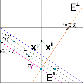
Figure 2: Cut and projection method applied to find the solutions of the Diophantine equation given by Eq. (3). Here, the flux vector is chosen to give $\phi=\tan\alpha=2/3$.The set of parallel lines gives possible solutions for $\bm{F}(\phi)\cdot\bm{T}_{r}=r$ for each gap $r$. For example, $\bf{T}_{1}$ and $\bf{T}_{2}$ are solutions for $r=1$ and $r=2$, others are indicated by open circles. Notice the periodicity of the solutions. In general, the flux vector $F$ defines a parallel subspace $E^{||}$, while $E^{\perp}$ is a perpendicular subspace defined by $F^{\perp}$. Any point $\bm{X}$, indicated by a black dot, can be decomposed as $\bm{X}=\bm{X}^{||}+\bm{X}^{\perp}$. Valid solutions require $\bm{X}$ to have integer coordinates and $|\bm{X}^{\perp}|<1$. Physically, $\bm{X}^{\perp}$ is the band filling ratio $r/q$.

A perpendicular subspace $E^{\perp}$ is now defined, as indicated in Fig. 2. All possible solutions to the Diophantine are contained in the family of parallel lines $\bm{X}\cdot\bm{F}(\phi)=r$. This is equivalent to find all integer coordinates that are within the parallel lines $\bm{X}\cdot\bm{F}(\phi)=0$ and $\bm{X}\cdot\bm{F}(\phi)=q$. We will call this region as the ”band”.

To find the solution of the Diophanitine equation we must proceed as in the cut and projection method. The steps are the following,

1) Consider a square lattice in 2D, such that $\bm{X}=(n_{1},n_{2})$ with $n_{1},n_{2}$ any integer.

2) Choose points such that $\bm{X}\cdot\bm{F}(\phi)\leq q$.

3) Then identify $n_{1}=\sigma_{r}$ and $n_{2}=\tau_{r}$. It is easy to show that integer coordinates points $\bm{X}$ within the band satisfy Naumis ,

$$\tau_{r}=-\lfloor\phi\sigma_{r}\rfloor$$ (7)

where $\lfloor z\rfloor$ denotes the floor function of $z$. The floor function allows to select points $\bm{X}$ that fall inside the band. Thus gaps are labeled by the coordinates of a two dimensional lattice,

$$(\sigma_{r},\tau_{r})=(\sigma_{r},-\lfloor\phi\sigma_{r}\rfloor)$$ (8)

By using that any number $z$ can be written as $z=\lfloor z\rfloor+\{z\}$, where $\{z\}$ denotes the fractional part of $z$ (observe that a negative number -$x$, we have $\{-x\}=1-\{x\}$), we can express $\tau_{r}$ as,

$$r=q\{\phi\sigma_{r}\}$$ (9)

Eq. (9) can be inverted using the same methodology giving the Chern numbers as a function of the gap index,

$$\sigma_{r}=\left(\frac{q}{2}-q\{\phi r+\frac{1}{2}\}\right)\zeta$$ (10)

where $\zeta=(-1)^{q-p}$ determines the correct sign in order to have a positive band index $r$. We will refer to these two previous equations as the hull functions. Several properties are deduced from Eq. (9) and Eq. (10). For rational $\phi$,

1. The solutions are periodic up to a vector $(-q,p)$ , i.e., Cherns numbers have a period $q$ while $\tau_{r}$ has period $p$.

2. The solutions for conductance correspond to Cherns between $-q/2$ and $q/2$. This defines a “first Brillouin zone” for Cherns.

3. The solution $\bm{T}_{1}$ for $r=1$ always exists, since a Diophantine equation of the form $ax+by=1$ always has solution if $p$ and $q$ are relative primes.

4. Then all solutions are obtained from the $r=1$ solution. To show this, consider the solution for $r=1$. It satisfies,

   $$\bm{F}(\phi)\cdot\bm{T}_{1}=1$$ (11)

   multiplying this equation by $r$, it will satisfy the Diophanite equation Eq. (6). Then,

   $$\bm{T}_{r}=r\bm{T}_{1}$$ (12)

5. Combining the previous properties, the solutions are given by,

   $$\bm{T}_{r}=r\bm{T}_{1}+s\bm{F}^{\perp}$$ (13)

   where $s$ is chosen to have Cherns between $-q/2$ and $q/2$. This is equivalent to take solutions modulus $q$ in $\sigma_{r}$ and modulus $p$ in $\tau_{r}$.

If we think Eq. (9) as a function of $\phi$ for each integer $\sigma_{r}$, we obtain the Claro-Wannier map CW seen in Fig. II a), which can be compared with the original butterfly II b). Each line corresponds to a gap and the slope of the line gives the Chern number. Fig. II b) the Chern labeling on the butterfly Naumis . The sawtooth function $\{\sigma_{r}\phi\}$ has period $1/\sigma_{r}$, and thus can be used to warp a torus for each Chern number $\sigma_{r}$. So consider the map $\Phi=2\pi\phi$ and $\theta=2\pi{\sigma_{r}\phi}$ as a parametrization of the torus, in which $\Phi$ is the azimuth angle, known as the ”toroidal” direction, and $\theta$ is the ”poloidal” angle. In Fig. II c) we present the trajectories on the tours for first Chern numbers. Notice how Fig. II c) is obtained by projecting the Claro-Wannier diagram of Fig. II onto a torus. It is interesting to observe that trajectories crossings corresponding to Van Hove singularities existing at all band centers due to saddle points of the energy dispersion Naumis .

III Cut and projection: structure of quasicrystals and topological phases

The method exposed in the previous section turns out to be the same as one of the used to generate the structure of quasicrystals: the cut and projection method Steurer . For further reference, let us now revist this method. To build the structure of a quasicristal, consider points $\bm{X}$ in a $D$ dimensional space periodic lattice,

$$\bm{X}=\sum_{j=1}^{D}n_{j}\bm{\hat{e}}_{j}$$ (14)

where $\bm{\hat{e}}_{j}$ are the lattice vectors of a hypercubic ($D>3$), cubic ($D=3$) or square lattice ($D=2$). These lattice points are projected onto a subspace $E^{||}$ using a projection operator $\hat{\Pi}(\bm{X})$. This projection will be called $\bm{X}^{||}$. A perpendicular subspace $E^{\perp}$ to $E^{||}$ is now defined. Any point $\bm{X}$ is decomposed as $\bm{X}=\bm{X}^{||}+\bm{X}^{\perp}$, where $\bm{X}^{\perp}$ is the projection onto $E^{\perp}$. Not all points $\bm{X}$ are selected to build the quasicrystal. Instead, points $\bm{X}$ are selected by using a band function $W(\bm{X}^{\perp})$ such that an acceptance width is given in the $E^{||}$ space, resulting in,

$$\bm{R}=\hat{\Pi}(\bm{X})W(\bm{X}^{\perp})=\bm{X}^{||}W(\bm{X}^{\perp})$$ (15)

where,

$$W(\bm{X}^{\perp})=\left\{\begin{array}[]{c}1\text{ if }|\bm{X}^{\perp}|<1\\ 0\text{ if }|\bm{X}^{\perp}|\geq 1\end{array}\right.$$ (16)

Since the points $\bm{X}$ form a lattice in D dimensions, using the linearity of the operator, it easy to prove that points in the quasicrystal are given by,

$$\bm{R}=\left(\sum_{j=1}^{D}n_{j}\bm{q}_{j}\right)W(n_{1},n_{2},...,n_{D})$$ (17)

where $n_{j}$ are integers and $\bm{q}_{j}$ is the projection of the higher-dimensionality base into $E^{||}$, i.e., $\bm{q}_{j}=\hat{\Pi}(\bm{\hat{e}}_{j})$.

Let us now use this method to build one dimensional quasicrystals and rational approximants. As explained in Fig. 2, we first consider a square-lattice. The subspace $E^{||}$ is now a line inclined with angle $-\alpha$, while $E^{\perp}$ is a line perpendicular to it.

The points $\bm{X}$ in 2D with integer coordinates have the form $\bm{X}\equiv\bm{X}_{n_{1},n_{2}}=(n_{1},n_{2})$. The projection in $E^{||}$ is given by,

$$\bm{X}^{||}\equiv\bm{X}_{n_{1},n_{2}}^{||}=n_{1}q_{1}-n_{2}q_{2}$$ (18)

where,

$$q_{1}=\cos\alpha=\frac{q}{\sqrt{p^{2}+q^{2}}};\ q_{2}=\sin\alpha=\frac{p}{\sqrt{p^{2}+q^{2}}}$$ (19)

and the perpendicular,

$$\bm{X}^{\perp}\equiv\bm{X}_{n_{1},n_{2}}^{\perp}=n_{1}q_{2}+n_{2}q_{1}$$ (20)

From this, the band condition (16) results here in a relationship between $n_{1}$ and $n_{2}$, to give $W(\bm{X}^{\perp})=\delta_{n_{1},-\lfloor n_{1}\tan\alpha\rfloor}$, with $\delta_{ij}$ is the Kronecker delta of $i$ and $j$. Finally, using the projection of the basis vectors $\bm{\hat{e}}_{1}=(1,0)$ and $\bm{\hat{e}}_{2}=(0,1)$ into the line $E^{||}$, we obtain the positions along the sequence,

$$R_{n_{1}}\equiv\bm{X}_{n_{1},n_{2}}^{||}W(\bm{X}_{n_{1},n_{2}}^{\perp})=n_{1}q_{1}+\lfloor n_{1}\tan\alpha\rfloor q_{2}$$ (21)

For irrational $\tan\alpha$, the sequence is quasiperiodic. The famous Fibonacci chain is obtained by using $\tan\alpha=\tau^{-1}$, where $\tau^{-1}=(\sqrt{5}-1)/2$ is the inverse golden mean. This method can be adapted to generate quasicrystals in 2D and 3D by using apropiate analytical expressions for the window function NaumisAragon1 ; NaumisAragon .

It is worthwhile mentioning that $R$ can be written as an average periodic chain, plus a flutuation part. Using the identity $x=\lfloor x\rfloor+\{x\}$

$$R_{n_{1}}=n_{1}<q>-\{n_{1}\tan\alpha\}q_{2}$$ (22)

where $<q>=q_{1}+\tan\alpha q_{2}$ is an average lattice parameter and the fractional part is the fluctuation part. The distances between consecutive points is given by,

$$|\delta R_{n_{1}}|=[\{(n_{1}+1)\tan\alpha\}-\{n_{1}\tan\alpha\}]q_{2}$$ (23)

Notice that other approximants or quasicrystals in the same local isomorphism class can be obtained by performing a translation of the width function along $E^{\perp}$. These extra degrees of freedom are known as phasons, which are related with the extra phases that appear in the Fourier transform when compared with a normal crystal. If the shift along $E^{\perp}$ is $\kappa$, then the sequence is transformed into,

$$R_{n_{1}}=n_{1}q_{1}+\lfloor n_{1}\tan\alpha+\kappa\rfloor q_{2}$$ (24)

or written as an average plus a fluctuation,

$$R_{n_{1}}=\kappa q_{2}+n_{1}<q>-\{n_{1}\tan\alpha+\kappa\}q_{2}$$ (25)

which shows that the effect is a shift of the origin.

Now we can see how the topological phases of the Hofstadter butterfly are determined by the same method used to build quasicrystal. We set $\tan\alpha=\phi$ and consider a higher-dimensional point $\bm{X}=\bm{X}_{\sigma_{r},\tau_{r}}=(\sigma_{r},\tau_{r})$ representing a possible topological phase. The distance between this topological phase point and the line $E^{||}$ is given by,

$$|\bm{X}_{\sigma_{r},\tau_{r}}^{\perp}|=\frac{\bm{X}_{\sigma_{r},\tau_{r}}\cdot\bm{F}(\phi)}{|\bm{F}(\phi)|}$$ (26)

and by using Eq. (8), we obtain,

$$|\bm{X}_{\sigma_{r},\tau_{r}}^{\perp}|=\frac{r}{\sqrt{p^{2}+q^{2}}}=\frac{q}{\sqrt{p^{2}+q^{2}}}\{\sigma_{r}\phi\}$$ (27)

Thus $|\bm{X}_{\sigma_{r},\tau_{r}}^{\perp}|$ determines the filling fraction $r/q$. From the previous equation, is clear a deep connection between the method to build quasicrystals and topological phases. We will explore such connections in the forthcoming sections,

IV Band conductance as a symbolic sequence

Let us first explain how the conductance is related with symbolic sequences akin to the structure of quasicrystals and its rational approximants. In general, the contribution of a band $r$ to the conductance is given by the difference between the Chern numbers associated with each band edge Fradkin ,

$$\sigma_{B}(r)=(\sigma_{r+1}-\sigma_{r})$$ (28)

where here the band and gap conductance is measured in units of $\frac{e}{h}$. By using Eq. (10) in the previous definition, we obtain that,

$$\sigma_{B}(r)=q\left(\{\phi r+\frac{1}{2}\}-\{\phi(r+1)+\frac{1}{2}\}\right)$$ (29)

This is precisely the distance between consecutive points in a sequence obtained from the cut and projection methods as in Eq. (25), i.e., is the set of distances between points in a rational approximant or in a quasicrystal. To see this, observe that the function $\{x\}$ has the property $\{a+b\}=\{a\}+\{b\}$ if $\{a\}+\{b\}<1$ and $\{a+b\}=1-(\{a\}+\{b\})$ if $\{a\}+\{b\}>1$. Thus, it turns out that $\sigma_{B}(r)$ only takes two values, $-p$ and $-q$. We map these two values to the letters $L$ and $S$. For $\zeta=1$,i.e., $q-p$ odd,

$$-p\rightarrow S$$ (30)

$$(q-p)\rightarrow L$$ (31)

while for $\zeta=-1$, i.e., $q-p$ even,

$$p\rightarrow S$$ (32)

$$(p-q)\rightarrow L$$ (33)

In Fig. 3 we show some sequences on the original Hofstadter butterfly. For each rational $\phi$, the periodicity of the sequence is given by $q$. In fact, by comparing Eqns. (28) and (23) and setting $\kappa=1/2$, we just proved that the band conductance is proportional to the fluctuation part of the sequence,

$$\sigma_{B}(r)=\delta R_{r+1}$$ (34)

To further understand the previous results, let us denote the band conductance sequences for a given $\phi$ as $S_{B}(\phi)$. In table 1 we show for several fluxes, the gap index $r$ and its associated Chern number $\sigma_{r}$, as well as the band conductances and the corresponding symbolic sequence. In these examples, each flux was chosen to match the first rational approximant of the golden mean $(\sqrt{5}-1)/2$, given by the ratio of two successive Fibonacci numbers $\phi_{j}=F(j-1)/F(j)$. The $j$-esim Fibonacci number is given by $F(j)=F(j-2)+F(j-1)$, with $F(0)=1$ and $F(1)=2$.

$\phi=1$  ($\zeta=1$)
$r$	$0$	$1$
$\sigma_{r}$	$0$	$1$
$\sigma_{B}(r)$	$1$	$-$
$S(1)$	L	-

$\phi=1/2$  ($\zeta=-1$)
$r$	$0$	$1$	$2$
$\sigma_{r}$	$0$	$-1$	$0$
$\sigma_{B}(r)$	$-1$	$1$	-
$S(1/2)$	L	S	-

$\phi=2/3$  ($\zeta=-1$)
$r$	$0$	$1$	$2$	$3$
$\sigma_{r}$	$0$	$-1$	$1$	0
$\sigma_{B}(r)$	$-1$	$2$	$-1$	-
$S(2/3)$	L	S	L	-

$\phi=3/5$  ($\zeta=1$)
$r$	$0$	$1$	$2$	$3$	$4$	$5$
$\sigma_{r}$	$0$	$2$	$-1$	$1$	$-2$	$0$
$\sigma_{B}(r)$	$2$	$-3$	$2$	$-3$	$2$	$-$
$S(3/5)$	L	S	L	S	L	$-$

$\phi=5/8$  ($\zeta=-1$)
$r$	$0$	$1$	$2$	$3$	$4$	$5$	$6$	$7$	$8$
$\sigma_{r}$	$0$	$-3$	$2$	$-1$	$-4$	$1$	$-2$	$3$	$0$
$\sigma_{B}(r)$	$-3$	$5$	$-3$	$-3$	$5$	$-3$	$-5$	$-3$	$-$
$S(5/8)$	L	S	L	L	S	L	S	L	-

Table 1: Gap number $r$, the associated Chern number $\sigma_{r}$, the band conductance given by $\sigma_{B}(r)=\sigma_{r+1}-\sigma_{r}$ and the associated symbolic sequence $S(\phi)$ for fluxes chosen as the first golden mean approximants. Notice how a given symbolic sequence is given by joining the previous two sequences. Such construction is seen in Figures 3 and 5, where bands conductances follow the same pattern. Also observe that sequences are similar to the usual Fibonacci ones up to a global phason due to the factor $1/2$ that appears in Eq. (28). Here all sequences are the same as in Fibonacci except for $\phi=3/5$.

As predicted by Eq. (29), a symbolic sequence is obtained for the band conductances. Moreover, we observe that in fact, the sequences for different fluxes also follow a recursive relation similar to the used for Fibonacci chains, i.e., form Table 1 we see that,

$$S(\phi_{j})=S(\phi_{j}-2)\oplus S(\phi_{j}-1)$$ (35)

where the sign $\oplus$ means join two sequences. From example, $S(5/8)=S(2/3)\oplus S(3/5)$. Although superficially this seems to be a Fibonacci sequence, in fact is very important to remark that the order of joining chains $S(\phi_{j}-2)\oplus S(\phi_{j}-1)$ is reversed when compared to the usual Fibonacci chain in which $S(\phi_{j}-1)\oplus S(\phi_{j}-2)$. For example, in Table 1 we see that the sequence for $\phi=3/5$ is $LSLSL$ while the Fibonacci is $LSLLS$. The reader may wonder why they are different or ”reversed”. The answer lies in the factor $1/2$ that appears in Eq. (28), this is equivalent to a global phason shift. However, in quasicrystals one needs to compare shifts of a sequence in order to decide if they are or not in the same isomorphism class NaumisPhason For example, we can apply several phason shifts to the sequence $LSLSL$. This is equivalent to an origin shift with cyclic boundary conditions. We obtain $LSLSL\rightarrow LLSLS\rightarrow SLLSL\rightarrow LSLLS$. Now the last sequence is the usual Fibonacci sequence and thus both sequences are in the same isomorphism class.

As is well known, an alternative way to generate such sequences is by using either deflation, inflation or recursive rulesLevine ; Steurer . The important result here is that we can relate different fluxes by such deflation/inflation rules. In Fig. 3 we explain the previous constructions on the original Hofstadter butterfly. Fig. 3 is meant to be compared with the sequence of Table 1.

Clearly, for other rational sequences as for the silver, bronce, etc. means, one can build such rules, and in fact, the general inflation/deflation rules generated by Eq. (29) have been extensively studied in the context of quasicrystals Levine ; Steurer .

In fact, a neat and suggestive way to write the symbolic sequences associated with each $\phi$ is by using $1$ and $0$ instead of $L$ and $S$. This is done by observing that,

$$S(\phi)=\left[sgn\left(\{\phi r+\frac{1}{2}\}-\{\phi(r+1)+\frac{1}{2}\}\right)+1\right]/2$$ (36)

where $sgn(x)$ is the algebraic sign of $x$ ($+1$ or $-1$) for $x\neq 0$ ($sgn(0)$ is defined as $0$). The previous equation can be interpreted as engineers do by looking at $r$ as a continuous variable, say the time, and $S(\phi)$ a square wave with period $\phi$ sampled with frequency one. A dynamical map can be assigned to such sequence,

$$S(\phi)=\left\{\begin{array}[]{cc}1&\text{if}\ \{\phi r+\frac{1}{2}\}<\phi\\ 0&\text{otherwise}\end{array}\right.$$ (39)

Both the symbolic sequence or the dynamical map gives what is called the Sturmian coding of a number Sturm , in this case $\phi$. The Sturmian coding is an alternative to the continued fraction approach which is very valuable in order to find good approximants of irrational numbers. The Sturmian coding can be easily visualized by a variant of the cut and projection. Take a square lattice, draw a line with slope $\phi$. As seen in Fig. 4 a), each intersection of this line with the verticals of the square lattice is labeled as a $0$, and each intersection with an horizontal line is labeled $1$. The labeling of the crossings is the Sturmian coding of $\phi$. Notice how in Fig. 4 a) the global phason shift discussed before turns out to be very clear. By shifting the line vertically we obtain the green line that produces a global shift of the chain, which is the one that needs to be compared with the Hofstadter butterfly conductance. For irrational $\phi$, the associated sequence is aperiodic and results in a Sturmian word Sturm .

Trajectories on the square lattice can also be warped into a torus or can be seen as a billard in which a particle with constant speed is reflected at the walls Bedaride . Each $0$ or $1$ is obtained by recording the collision with horizontal or vertical walls of a trajectory with initial slope $\phi$. Fig. 4 b) indicates such procedure.

The spectrum of the map defined by Eq. (39) is made with discrete frequences $f_{s,l}$ and amplitudes $\tilde{S}_{l}(\phi)$ given by,

$$\tilde{S}_{l}(\phi)=\frac{sin(\pi l\phi)}{\pi l},\hskip 170.71652ptf_{sl}=s+l\phi$$ (40)

The proposed scheme can also be used to characterize other systems, like the square well potential which contains as a special case, the Fibonacci chain potential NaumisPHYSB . As seen in Fig. 5, this allows to produce a Fibonacci butterfly . It has been shown that such potential is in the same topological class as the Hofstadter butterfly QCti . Thus, all of the methodology developed here can be applied. As an example, in Fig. 5 we indicate the same symbolic sequences for the band conductances seen in Fig. 3.

In Figs. 3 and 5, it is interesting to observe that band conductances are related to band widths. This can be understood in terms of general arguments concerning the electron’s wavefunction overlap in systems that are rational approximants to quasicrystals NaumisTrace . In fact, a dynamical map can be used to investigate the scaling exponents for critical states, and relate them with band-width scaling NaumisTrace ; NaumisJP .

Figure 3: Some symbolic sequences for bands conductance given in table 1, over imposed on the Hofstadter butterfly. Bands with index L are indicated in blue, while bands with S are in red. The sequence for $\phi=3/5$ is obtained by joining the sequences $\phi=1/2$ and $\phi=2/3$, as indicated at the figure top and by the green boxes. Notice the inflation/deflation rules and the scaling of bands.

Figure 4: Panel a), Sturmian coding of $\phi=3/5$. The black line going through the origin is the usual Sturmian coding for a flux $\phi=3/5=0.618$. This is an approximant of the Golden mean. The slope of the inclined line is $\phi$. Each intersection is labeled as $0$ or $1$ depending on the kind of intersection with the grid. The displaced green line is the same sequence with a global phason shift, and can be compared with the sequence of Table 1. Observe how the color coding is the same as in the Hofstadter butterfly conductances seen at $\phi=3/5$ in Fig. 3. Panel b), the coding can be found in a square colored billiard, in which each kind of reflection, with a vertical or horizontal wall is coded with a $0$ or $1$. The reason is that one can fold the trajectory shown in panel a) by thinking each intersection with the grid as mirrors.

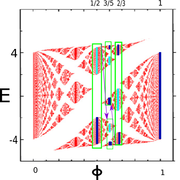
Figure 5: The same symbolic sequences for the fluxes seen in Fig. 3 over imposed on the Fibonacci butterfly, which is obtained by a square well potential NaumisPHYSB . Bands with index L are indicated in blue, while bands with S are in light blue. From this figure, the topological equivalence with the Hofstadter butterfly is clearly seen.

V Methods to calculate Chern numbers and global fractality

From the previous inflation/deflation rules is possible to reverse the procedure, i.e., to obtain the Chern numbers for each gap by a simple recurrence relation. This allows to bypass the need to solve a Diophantine equation. Such procedure is readly obtained from observing that the Chern number for a gap $r$ is the sum of all band conductances up to the given filling fraction Fradkin ,

$$\sigma_{r}=\sum_{s=1}^{r}\sigma_{B}(s)$$ (41)

from where,

$$\sigma_{r}=\sigma_{r-1}+\sigma_{B}(r)$$ (42)

It follows that we only need to find the two letter sequence and assign to each letter its numeric counterpart and then sum the sequence at each step. Let us show a simple example. Suppose that we want to calculate the Chern numbers for $\phi=5/8$ without solving the Diophantine equation. We simply use the Fibonacci rule $S(\phi_{j})=S(\phi_{j}-2)\oplus S(\phi_{j}-1)$ to produce the sequence $S(5/8)$,

$$S(5/8)=LSLLSLSL=-3,5,-3,-3,5,-3.-5,-3$$ (43)

where the last step requires the numerical equivalence of a letter, in this case $S\rightarrow-p$ and $L\rightarrow(q-p)$ as $q-p$ is odd. The sequence of Chern numbers is obtained by using the recurrence relationship Eq. (42) and the initial condition $\sigma_{0}=0$,

$$\sigma_{1}=0-3=-3\rightarrow\sigma_{2}=-3+5=2\rightarrow\sigma_{3}=2-3=-1\rightarrow\sigma_{4}=-1-3=-4$$ (44)

$$\sigma_{5}=-4+5=1\rightarrow\sigma_{6}=1-3=-2\rightarrow\sigma_{7}=-2+5=3\rightarrow\sigma_{8}=3-3=0.$$ (45)

A simple comparison with table 1 shows that the sequence is correct and valid for the Hofstadter and Fibonacci butterflies. If the recursion rule for sequence is not known, there are two options. The first is to build the Sturmian coding of $\phi$. The second option is much more efficient: use a simple recursive test. This option works as follows. Determine the sign $\zeta$. As always $\sigma_{0}=0$, the next Chern number $\sigma_{1}$ is either $\sigma_{0}-\zeta p$ or $\sigma_{0}+\zeta(q-p)$. A direct sustitution in the Diophantine equation gives the right choice. Once $\sigma_{1}$ is known, $\sigma_{2}$ can be calculated in a similar way. The method is iterated by using always the previous Chern number as a seed, i.e., $\sigma_{n+1}=\sigma_{n}-\zeta p$ or $\sigma_{n+1}=\sigma_{n}-\zeta(q-p)$.

Yet, there is another powerful method to find the Chern numbers. This method reveals several fractal properties of the butterfly. This method is based in the observation made is section II that solutions are obtained from $\bm{F}(\phi)\cdot\bm{T}_{1}=1$. With the vector $\bm{T}_{1}=(\sigma_{1},\tau_{1})$ we define a flux $\phi^{\prime}=-\tau_{1}/\sigma_{1}$, which turns out to be a Farey neighbor of $\phi$. The argument is follows; for two reduced fractions $\phi=p/q$ and $\phi^{\prime}=p^{\prime}/q^{\prime}$, the mediant is defined as Schroeder ,

$$\frac{p^{\prime\prime}}{q^{\prime\prime}}=\frac{p+p^{\prime}}{q+q^{\prime}}$$ (46)

This requires the fractions to be unimodular $|p^{\prime}q-pq^{\prime}|=1$. Such construction is easily understood in two dimensions, as,

$$\bm{F}(\phi^{\prime\prime})=\bm{F}(\phi)+\bm{F}(\phi^{\prime})$$ (47)

and the condition for unimodularity is $\bm{F}(\phi)\cdot\bm{F}^{\perp}(\phi^{\prime})=\pm 1$. Thus we can identify the fundamental solution as,

$$\bm{T}_{1}=\bm{F}^{\perp}(\phi^{\prime})\hskip 28.45274pt\text{with}\hskip 28.45274pt\phi^{\prime}=-\tau_{1}/\sigma_{1}$$ (48)

Mediants occurs naturalley in Farey sequences, defined as fractions between $0$ and $1$ of a given largest denominator Schroeder . In this sequence, each fraction is the median of its two neighbors. Thus, we just proved that given a flux $\phi$, the fundamental solution is given by one of the Farey neighbors. Let us workout an example to reproduce some results of Table 1. Consider the Farey sequence of order 5 built from a Farey tree Schroeder ,

$$\frac{0}{1},\ \frac{1}{5},\ \frac{1}{4},\ \frac{1}{3},\ \frac{2}{5},\ \frac{1}{2},\ \frac{3}{5},\ \frac{2}{3},\ \frac{3}{4},\ \frac{4}{5},\ \frac{1}{1}$$ (49)

and apply it to the flux $\phi=2/3$. Its upper Farey neighbor $\phi^{\prime}=3/4$ satisfies $\bm{F}(2/3)\cdot\bm{F}^{\perp}(3/4)=(2,3)\cdot(-4,3)=1$ as expected for a Farey sequence. Thus we identify $\bm{F}^{\perp}(3/4)=\bm{T}_{1}=(-4,3)$. The solution can be folded back to the ”Chern first Brillouin zone” by taking the modulus with $\bm{F}^{\perp}(2/3)$ as explained in section II, from where $\bm{T}_{1}=(-4,3)+(3,-2)=(-1,1)$ resulting in $\sigma_{1}=-1$, coinciding with Table I. As a matter of fact, each flux in the Farey sequence provides all its own solutions by using its right neighbor fraction in the sequence. Its is important to remark that the approximants of the golden ratio, given by the Fibonacci numbers, are also Farey neighbors Schroeder .

These observations suggest the possibility to understand the self-similarity of the topological phase diagram by observing how phases are related at different fluxes. Indeed this is the case. Consider the vectorial sum Eq. (47) applied to the product,

$$\bm{F}(\phi^{\prime\prime})\cdot\bm{T}_{1}(\phi)=[\bm{F}(\phi)+\bm{F}(\phi^{\prime})]\cdot\bm{T}_{1}(\phi)$$ (50)

where now we changed the notation to indicate that $\bm{T}_{1}(\phi)$ is a fundamental solution for flux $\phi$, i.e.,$\bm{F}(\phi)\cdot\bm{T}_{1}(\phi)=1$, before doing the folding using the vector $\bm{F}^{\perp}(\phi)$. Using this fact and that $\bm{F}(\phi^{\prime})\cdot\bm{T}_{1}(\phi)=\bm{F}(\phi^{\prime})\cdot\bm{F}_{1}^{\perp}(\phi^{\prime})$, it follows that,

$$\bm{F}(\phi^{\prime\prime})\cdot\bm{T}_{1}(\phi)=1$$ (51)

proving that $\bm{T}_{1}(\phi)$ is a fundamental solution of the mediant $\phi^{\prime\prime}$ obtained from $\phi$ and $\phi^{\prime}$. It is important to remark that the solution can be folded to have Cherns between $q/2$ and $-q/2$ by using the rule $\bm{T}_{1}(\phi)-s\bm{F}^{\perp}(\phi^{\prime\prime})$ for some integer $s$.

Consider as an example the same flux $\phi=2/3$, with Farey neighbour $\phi^{\prime}=3/4$. The resulting mediant is $\phi^{\prime\prime}=(2+3)/(4+3)=5/7$. We have that,

$$\bm{F}(5/7)\cdot\bm{T}_{1}(2/3)=(5,7)\cdot(-4,3)=1$$ (52)

as predicted. By folding back by $\bm{F}^{\perp}(5/7)=(-7,5)$ it gives the fundamental solution $(3,-1)$, i.e., the first Chern for $\phi=5/7$ is $3$. It is important to remark that if we use the unfolded solution $\bm{T}_{1}(\phi)=(-1,1)$, instead of $(-4,3)$, we will not get the fundamental solution but a shifted one. This comes out as follows, let us consider again the product (50) but with a folding,

$$\bm{F}(\phi^{\prime\prime})\cdot(\bm{T}_{1}(\phi)+s\bm{F}^{\perp}(\phi))=1+s\bm{F}(\phi^{\prime})\cdot\bm{F}^{\perp}(\phi)$$ (53)

The product $\bm{F}(\phi^{\prime})\cdot\bm{F}^{\perp}(\phi)$ although being integer, is not zero in general, resulting in a solution different from $r=1$.

What is remarkable about Eq. (51) is that the sequence for a flux $\phi^{\prime\prime}$ is contained and generated by the same solution than $\phi$, as we can simply multiply Eq. (51) by $r$,

$$\bm{F}(\phi^{\prime\prime})\cdot[r\bm{T}_{1}(\phi)]=\bm{F}(\phi^{\prime\prime})\cdot[\bm{T}_{r}(\phi)]=r$$ (54)

where $\bm{T}_{r}(\phi)$ is the solution for gap $r$ for a $\phi$ which is above $\phi^{\prime\prime}$ in the Farey tree. Yet the folding is dictated by $\phi^{\prime\prime}$ instead of $\phi$. As a matter of fact, it means that we were able to find a construction based in blocks of sequences as happens with the Fibonacci ones, but this time, for any rational flux, as the Farey tree will eventually contain the fraction. Such construction can be seen in Figs. 3 and 5 for the fractions $1/2,3/5,2/3$. This helps to explain the previously numerically observed relationships between the global fractality of the butterfly and Farey neighbors sequences, as well as for its representation as Ford circles InduEPJ ; Indubook .

VI Harper potential and the cut and projection method

One may wonder what is behind the fact that the cut and projection method predicts the topological phases. The reason is that band gaps where topological modes reside, are open due to electron diffraction, as stationary waves are produced when the wavevector $\bm{k}$ is equal to a reciprocal lattice vector $\bm{Q}$. Thus, a vanishing group velocity $\bm{v}_{g}(\bm{k})$ is observed and a Van Hove singularity occurs. Formally, band gaps and diffraction are related through the general formula for the density of states $\rho(\epsilon)$,

$$\rho(\epsilon)=\oint_{\bm{S}(\epsilon)}\frac{d\bm{S}}{2\pi^{2}|\bm{v}_{g}(\bm{k})|}$$ (55)

where $\epsilon$ is the energy and $\bm{k}$ the wavevector. The integral is made along contours $\bm{S}(\epsilon)$ of equal energy. The group velocity is determined by the energy dispersion $\bm{v}_{g}(\bm{k})=\nabla_{\bm{k}}\epsilon(\bm{k})$. Whenever diffraction occurs, $|\bm{v}_{g}(\bm{k})|=0$. The previous formula explains the Van Hove logarithm singularities and related topological collisions at each Hofstadter butterfly band center Naumis .

Let us now understand how the cut and projection method is related with bands. We start our analysis by using the identity $x=\lfloor x\rfloor+\{x\}$ applied to $m\phi+\nu_{y}$ in the Harper potential given in Eq. (1),

$$V(m)=2\lambda\cos(2\pi\{m\phi+\nu_{y}\})$$ (56)

Next we observe that lower band edges are obtained by seeting $\nu_{y}=0$ in Eq. (1). The other limiting value $\nu_{y}=1/2$ gives the upper band edges Thouless . As we are only interested in states at band edges, in whatfollows we will only consider lower band edges $\nu_{y}=0$ since upper band edges share the same Chern numbers as the contiguous lower band edge. In such case, using Eq. (9), we can reinterpret $m$ as a Chern number, i.e., $m=\sigma_{r}$, from where the fractional part can be associated with the band index,

$$V(\sigma_{r})=2\lambda\cos(2\pi\{\sigma_{r}\phi\}q/q)=2\lambda\cos(2\pi r/q)$$ (57)

Now is clear how the argument of the cosine is associated with a wave-vector $k=2\pi r/q$, having $r=0,...,q-1$. Furthermore, using Eq. (57) and Eq. (27), it follows that,

$$V(\sigma_{r})=2\lambda\cos(2\pi\sqrt{p^{2}+q^{2}}|\bm{X}_{\sigma_{r},\tau_{r}}^{\perp}|)$$ (58)

Also, as $|\bm{X}_{\sigma_{r},\tau_{r}}^{\perp}|<1$, this shows that $V(\bm{\sigma_{r}})$ induces an ordering of the potential according to its distances in $E^{\perp}$. Since band-level crossings do not happen Fradkin , the ordering is preserved for all $\lambda$. Alternatively, we can say that ordering is provided by the Chern number map of Eq. (27).

Let us explain in detail the previous assertion. Following Fradkin Fradkin , consider the limit $\lambda\rightarrow\infty$. Then $\psi_{m}^{r}\approx\delta(m-m_{r})$, i.e., the wave function is a delta centered at some site $m_{r}$ for band $r$. To find where is it localized, from Eq. (1) this will happen whenever the energy of the level is,

$$E_{r}\approx V(m_{r})=2\lambda\cos(2\pi\{m_{r}\phi\}q/q)$$ (59)

Setting $m_{r}=\sigma_{r}$ we obtain,

$$E_{r}\approx 2\lambda\cos(2\pi r/q)=2\lambda\cos(2\pi\sqrt{p^{2}+q^{2}}|\bm{X}_{\sigma_{r},\tau_{r}}^{\perp}|)$$ (60)

The process can be summarized as follows. For a band $r$, the state is localized at site $m_{r}=\sigma_{r}$. Or in an alternative way, given a site $m_{r}=\sigma_{r}$, its associated band position is determined by $|\bm{X}_{\sigma_{r},\tau_{r}}^{\perp}|$.

Notice that due to the parity of $V(m)$, the localization can also happen at $m=-\sigma_{r}$ for the same energy. Since for a rational $\phi$ the lattice is periodic, $m$ needs to be folded back into sites $m=0,...,q-1$. By performing the right folding depending wheter $q$ is odd or even, one finds that the delta functions are separated by a Chern number of sites, and results in the Chern phenomena beating discovered in Ref. InduPRL . This phenomena implies that edge states for each band are a convolution of the Chern doublets with the ground state. For the case of $\lambda=1$, the doublet is convoluted with a fractal ground state resulting in fractal doubletsInduPRL .

Also, Aubry and Andre proved that the Harper equation is self-reciprocal Harper , i.e, the Fourier coefficients of the wave-function follow the same Harper equation but with $\lambda$ replaced using the rule $\lambda\rightarrow 1/\lambda$. As a result, for $\lambda\rightarrow 0$, the Fourier coefficients of the wave-function are just delta-localized at $k=\pm\sigma_{r}$ resulting in the wave-function,

$$\psi_{m}^{r}\approx\frac{1}{q}cos(2\pi\sigma_{r}m)$$ (61)

for the band $r$.

Here we proved that the map $r=\{\sigma_{r}\phi\}q$ allows to order the energies in terms of the potential $V(\sigma_{r})$, and this ordering is the same as the one for the wave-function Fourier coefficients. We can also reinterpret Eq. (57) in the original framework proposed by Hofstadter, i.e. the Bloch-Floquet theorem for the wave-function in real space leads to just a re-ordering in reciprocal space for the original wave-functions Hof . The order is dictated by the perpendicular component of $\bm{X}$.

It is worthwhile mentioning that around a given flux, several topological sequences can be obtained by tilting Naumis $\phi$ by a small amount $\delta\phi$. This is equivalent to introduce phason disorder, and as a consequence, the resulting sequences have satellites in the diffraction pattern NaumisPhason . Similar patterns are observed on graphene over a sustrate Taboada ; TaboadaRipple .

VII Conclusions

Using ideas from quasicrystals, in particular the cut and projection method, we were able to find several interesting properties of the Diophantine equation which characterizes the Hofstadter butterfly as a topological phase diagram. We showed that the bands conductance for any given rational flux are described by symbolic sequences. Thus, bands conductance at different fluxes can be related by inflation/deflation rules as happens for rational approximants of quasiperiodic sequences. Such rules correspond to the Sturmian sequence of the flux. They can be obtained by using a dynamical map, a trajectory in a torus or in a square billiard, resulting in easy rules to find Chern numbers. The presented mechanism is also valid for the square well potential which leads to the Fibonacci butterfly NaumisPHYSB . We also have a higher dimensional construction that allows to find solutions and its self-similarity through Farey sequences, trees and neighbours. This allows to describe topological phases within the context of quasicrystals, which is seems to be useful in order to describe complex phases in Moire patterns of graphene over graphene at magical angles Tarnopolsky2019 .

This work has been supported by UNAM-DGAPA project IN102717.

References

- (1) D. J.Thouless,M.Kohmoto,M. P.Nightingale and M. den Nijs, PRL, 49, 405 (1982).
- (2) D. Hofstadter, Phys Rev B, 14 2239 (1976).
- (3) C. R. Dean and L. Wang and L. Maher and P. Forsythe and F. Ghahari and F. and Y. Gao and Katoch, J. Ishigami and M. Moon and P. Koshino and M. Taniguchi and T. Watanabe and K. Shepard and K. L. J. Hone and P. Kim, Nature, 497, 598, (2013).
- (4) Tarnopolsky, Grigory and Kruchkov, Alex Jura and Vishwanath, Ashvin, Phys. Rev. Lett., 122, 106405, (2019)
- (5) C.L. Kane and E. J. Mele, Phys Rev Lett, 95 146802 (2005).
- (6) M. Z.Hasan and C. L.Kane, Rev.Mod.Phys. 82 3045 (2010)
- (7) G.G Naumis, P Roman-Taboada Phys. Rev. B 89 , 241404 (2014)
- (8) G.G. Naumis, S. Barraza, M. Oliva-Leyva. H. Terrones, Rep. Prog. Phys. 9, 80 (2017)
- (9) Rami Ahmad El-Nabulsi, Journal of Physics and Chemistry of Solids, 127, 224-230 (2019).
- (10) Igor N. Karnaukhov, Physics Letters A 383, 2114-2119, (2019).
- (11) E. Fradkin, Field Theories of Condensed Matter Systems, 2nd Edition. Cambridge University Press, Cambridge (2013).
- (12) Hua-Ling Yu, Zhang-Yin Zhai, Xin-Tian Bian, Chinese Phys. Lett. 33, 117305 (2016).
- (13) H. L. Yu and Z. Y. Zhai, Modern Physics Letters B, 32, 1850158, (2018).
- (14) I.N. Karnaukhov, J. Phys. Commun. 1, 051001 (2017).
- (15) I. Satija, Butterfly in the Quantum World: The story of the most fascinating quantum fractal, Morgan Claypool Publishers, San Rafael, CA (2016).
- (16) I. satija, Eur. Phys. J. Special Topics225, 2533–2547 (2016).
- (17) S. Aubry and G. Andre, Ann. Isr. Phys. Soc. 3, 133 (1980).
- (18) S. Ostlund and R. Pandit, Phys Rev B, 29 1394 (1984).
- (19) I. Dana, Y. Avron and J. Zak, J. Phys. C, Solid State Phys 18 (1985) L679.
- (20) C. Janot, Quasicrystals (Clarendon, Oxford, 1994), 2nd ed.
- (21) Crystallography of Quasicrystals, W. Steurer, S. Deloudi, Springer Verlag, Berlin , Springer Series in Materials Sciences 126, (2009).
- (22) G.G. Naumis, F.J. López-Rodríguez, Physica B 403, 1755 (2008).
- (23) Yaacov E. Kraus and Oded Zilberberg, Phys. Rev. Lett., 109, 116404 (2012)
- (24) Yaacov E. Kraus, Yoav Lahini,Zohar Ringel,Mor Verbin, and Oded Zilberberg, PRL, 109 106402 (2012)
- (25) I. Satja, G.G. Naumis, Phys. Rev. B 88, 054204 (2013).
- (26) D. Levine, P.J. Steinhardt, Phys. Rev. B 34, 596 (1986).
- (27) G.G. Naumis, Phys. Rev. B 71, 144204 (2005).
- (28) G. G. Naumis, Phys. Lett. A 380 1772-1780, (2016).
- (29) F. H. Claro, W. H. Wannier, Phys. Rev. B 19 (1979) 6068-74.
- (30) Hatsugai and Kohmoto, Phys Rev B, 42, (1990), 8282
- (31) Substitutions in Dynamics, Arithmetics and Combinatorics, V. Berthé, S. Ferenczi, C. Mauduit, A. Siegel, Series Lecture Notes in Mathematics, Springer Verlag, Berlín, (2002)
- (32) N. Bedaride, Theoretical Computer Science 385, 214–225 (2007).
- (33) G.G Naumis Physical Review B 59 , 11315 (1999)
- (34) G.G Naumis, J. Phys: Condens. Matter 15, 5969 (2003).
- (35) M. Schroeder, Fractals, Chaos, Power Laws, Dover, New York (2009).
- (36) D. Thouless, Phys. Rev. B 28, 4272 (1983).
- (37) G.G Naumis, C Wang, MF Thorpe, RA Barrio Physical Review B 59 , 14302 (1999).
- (38) P Roman-Taboada, G.G Naumis Physical Review B 90, 195435 (2014).
- (39) G.G Naumis; Aragon, JL, Zeitschrift für Kristallographie, 218, 397 (2003).
- (40) J.L. Aragón, G.G. Naumis, M. Torres, Acta Cryst. A58, 352-360 (2002).
- (41) G.G Naumis, Phys. Rev. B 71, 144204 (2005).