Flexibly Fair Representation Learning by Disentanglement
Abstract
We consider the problem of learning representations that achieve group and subgroup fairness with respect to multiple sensitive attributes. Taking inspiration from the disentangled representation learning literature, we propose an algorithm for learning compact representations of datasets that are useful for reconstruction and prediction, but are also flexibly fair, meaning they can be easily modified at test time to achieve subgroup demographic parity with respect to multiple sensitive attributes and their conjunctions. We show empirically that the resulting encoder—which does not require the sensitive attributes for inference—enables the adaptation of a single representation to a variety of fair classification tasks with new target labels and subgroup definitions.
1 Introduction
Machine learning systems are capable of exhibiting discriminatory behaviors against certain demographic groups in high-stakes domains such as law, finance, and medicine (Kirchner et al., 2016; Aleo & Svirsky, 2008; Kim et al., 2015). These outcomes are potentially unethical or illegal (Barocas & Selbst, 2016; Hellman, 2018), and behoove researchers to investigate more equitable and robust models. One promising approach is fair representation learning: the design of neural networks using learning objectives that satisfy certain fairness or parity constraints in their outputs (Zemel et al., 2013; Louizos et al., 2016; Edwards & Storkey, 2016; Madras et al., 2018). This is attractive because neural network representations often generalize to tasks that are unspecified at train time, which implies that a properly specified fair network can act as a group parity bottleneck that reduces discrimination in unknown downstream tasks.
Current approaches to fair representation learning are flexible with respect to downstream tasks but inflexible with respect to sensitive attributes. While a single learned representation can adapt to the prediction of different task labels , the single sensitive attribute for all tasks must be specified at train time. Mis-specified or overly constraining train-time sensitive attributes could negatively affect performance on downstream prediction tasks. Can we instead learn a flexibly fair representation that can be adapted, at test time, to be fair to a variety of protected groups and their intersections? Such a representation should satisfy two criteria. Firstly, the structure of the latent code should facilitate simple adaptation, allowing a practitioner to easily adapt the representation to a variety of fair classification settings, where each task may have a different task label and sensitive attributes . Secondly, the adaptations should be compositional: the representations can be made fair with respect to conjunctions of sensitive attributes, to guard against subgroup discrimination (e.g., a classifier that is fair to women but not Black women over the age of 60). This type of subgroup discrimination has been observed in commercial machine learning systems (Buolamwini & Gebru, 2018).
In this work, we investigate how to learn flexibly fair representations that can be easily adapted at test time to achieve fairness with respect to sets of sensitive groups or subgroups. We draw inspiration from the disentangled representation literature, where the goal is for each dimension of the representation (also called the “latent code”) to correspond to no more than one semantic factor of variation in the data (for example, independent visual features like object shape and position) (Higgins et al., 2017; Locatello et al., 2019). Our method uses multiple sensitive attribute labels at train time to induce a disentangled structure in the learned representation, which allows us to easily eliminate their influence at test time. Importantly, at test time our method does not require access to the sensitive attributes, which can be difficult to collect in practice due to legal restrictions (Elliot et al., 2008; DCCA, 1983). The trained representation permits simple and composable modifications at test time that eliminate the influence of sensitive attributes, enabling a wide variety of downstream tasks.
We first provide proof-of-concept by generating a variant of the synthetic DSprites dataset with correlated ground truth factors of variation, which is better suited to fairness questions. We demonstrate that even in the correlated setting, our method is capable of disentangling the effect of several sensitive attributes from data, and that this disentanglement is useful for fair classification tasks downstream. We then apply our method to a real-world tabular dataset (Communities & Crime) and an image dataset (Celeb-A), where we find that our method matches or exceeds the fairness-accuracy tradeoff of existing disentangled representation learning approaches on a majority of the evaluated subgroups.
2 Background
Group Fair Classification
In fair classification, we consider labeled examples where are labels we wish to predict, are sensitive attributes, and are non-sensitive attributes. The goal is to learn a classifier (or ) which is predictive of and achieves certain group fairness criteria w.r.t. . These criteria are typically written as independence properties of the various random variables involved. In this paper we focus on demographic parity, which is satisfied when the predictions are independent of the sensitive attributes: . It is often impossible or undesirable to satisfy demographic parity exactly (i.e. achieve complete independence). In this case, a useful metric is demographic parity distance:
| (1) |
where here is a binary prediction derived from model output . When , demographic parity is achieved; in general, lower implies less unfairness.
Our work differs from the fair classification setup as follows: We consider several sensitive attributes at once, and seek fair outcomes with respect to each; individually as well as jointly (cf. subgroup fair classification, Kearns et al. (2018); Hebert-Johnson et al. (2018)); also, we focus on representation learning rather than classification, with the aim of enabling a range of fair classification tasks downstream.
Fair Representation Learning
In order to flexibly deal with many label and sensitive attribute sets, we employ representation learning to compute a compact but predicatively useful encoding of the dataset that can be flexibly adapted to different fair classification tasks. As an example, if we learn the function that achieves independence in the representations with or , then any predictor derived from this representation will also achieve the desired demographic parity, with .
The fairness literature typically considers binary labels and sensitive attributes: . In this case, approaches like regularization (Zemel et al., 2013) and adversarial regularization (Edwards & Storkey, 2016; Madras et al., 2018) are straightforward to implement. We want to address the case where is a vector with many dimensions. Group fairness must be achieved for each of the dimensions in (age, race, gender, etc.) and their combinations.
VAE
The vanilla Variational Autoencoder (VAE) (Kingma & Welling, 2013) is typically implemented with an isotropic Gaussian prior . The objective to be maximized is the Evidence Lower Bound (a.k.a., the ELBO),
which bounds the data log likelihood from below for any choice of . The encoder and decoder are often implemented as Gaussians
whose distributional parameters are the outputs of neural networks , , , , with the typically exhibiting diagonal structure. For modeling binary-valued pixels, a Bernoulli decoder can be used. The goal is to maximize —which is made differentiable by reparameterizing samples from —w.r.t. the network parameters.
-VAE
Higgins et al. (2017) modify the VAE objective:
The hyperparameter allows the practitioner to encourage the variational distribution to reduce its KL-divergence to the isotropic Gaussian prior . With this objective is a valid lower bound on the data likelihood. This gives greater control over the model’s adherence to the prior. Because the prior factorizes per dimension , Higgins et al. (2017) argue that increasing yields “disentangled” latent codes in the encoder distribution . Broadly speaking, each dimension of a properly disentangled latent code should capture no more than one semantically meaningful factor of variation in the data. This allows the factors to be manipulated in isolation by altering the per-dimension values of the latent code. Disentangled autoencoders are often evaluated by their sample quality in the data domain, but we instead emphasize the role of the encoder as a representation learner to be evaluated on downstream fair classification tasks.
FactorVAE and -TCVAE
Kim & Mnih (2018) propose a different variant of the VAE objective:
The main idea is to encourage factorization of the aggregate posterior so that correlates with if and only if . The authors propose a simple trick to generate samples from the aggregate posterior and its marginals using shuffled minibatch indices, then approximate the term using the cross entropy loss of a classifier that distinguishes between the two sets of samples, which yields a mini-max optimization.
Chen et al. (2018) show that the term above—a.k.a. the “total correlation” of the latent code—can be naturally derived by decomposing the expected KL divergence from the variational posterior to prior:
They then augment the decomposed ELBO to arrive at the same objective as Kim & Mnih (2018), but optimize using a biased estimate of the marginal probabilities rather than with the adversarial bound on the KL between aggregate posterior and its marginals.
3 Related Work
Most work in fair machine learning deals with fairness with respect to single (binary) sensitive attributes. Multi-attribute fair classification was recently the focus of Kearns et al. (2018)—with empirical follow-up (Kearns et al., 2019)—and Hebert-Johnson et al. (2018). Both papers define the notion of an identifiable class of subgroups, and then obtain fair classification algorithms that are provably as efficient as the underlying learning problem for this class of subgroups. The main difference is the underlying metric; Kearns et al. (2018) use statistical parity whereas Hebert-Johnson et al. (2018) focus on calibration. Building on the multi-accuracy framework of Hebert-Johnson et al. (2018), Kim et al. (2019) develop a new algorithm to achieve multi-group accuracy via a post-processing boosting procedure.
The search of independent latent components that explain observed data has long been a focus on the probabilistic modeling community (Comon, 1994; Hyvärinen & Oja, 2000; Bach & Jordan, 2002). In light of the increased prevalence of neural networks models in many data domains, the machine learning community has renewed its interest in learned features that “disentangle” semantic factors of data variation. The introduction of the -VAE (Higgins et al., 2017), as discussed in section 2, motivated a number of subsequent studies that examine why adding additional weight on the KL-divergence of the ELBO encourages disentangled representations (Alemi et al., 2018; Burgess et al., 2017). Chen et al. (2018); Kim & Mnih (2018) and Esmaeili et al. (2019) argue that decomposing the ELBO and penalizing the total correlation increases disentanglement in the latent representations. Locatello et al. (2019) conduct extensive experiments comparing existing unsupervised disentanglement methods and metrics. They conclude pessimistically that learning disentangled representations requires inductive biases and possibly additional supervision, but identify fair machine learning as a potential application where additional supervision is available by way of sensitive attributes.
Our work is the first to consider multi-attribute fair representation learning, which we accomplish by using sensitive attributes as labels to induce a factorized structure in the aggregate latent code. Bose & Hamilton (2018) proposed a compositional fair representation of graph-structured data. Kingma et al. (2014) previously incorporated (partially-observed) label information into the VAE framework to perform semi-supervised classification. Several recent VAE variants have incorporated label information into latent variable learning for image synthesis (Klys et al., 2018) and single-attribute fair representation learning (Song et al., 2019; Botros & Tomczak, 2018; Moyer et al., 2018). Designing invariant representations with non-variational objectives has also been explored, including in reversible models (Ardizzone et al., 2019; Jacobsen et al., 2019).
4 Flexibly Fair VAE
We want to learn fair representations that—beyond being useful for predicting many test-time task labels —can be adapted simply and compositionally for a variety of sensitive attributes settings after training. We call this property flexible fairness. Our approach to this problem involves inducing structure in the latent code that allows for easy manipulation. Specifically, we isolate information about each sensitive attribute to a specific subspace, while ensuring that the latent space factorizes these subspaces independently.
Notation
We employ the following notation:
-
•
: a vector of non-sensitive attributes, for example, the pixel values in an image or row of features in a tabular dataset;
-
•
: a vector of binary sensitive attributes;
-
•
: non-sensitive subspace of the latent code;
-
•
: sensitive subspace of the latent code111 In our experiments we used (same number of sensitive attributes as sensitive latent dimensions) to model binary sensitive attributes. But categorical or continuous sensitive attributes can also be accommodated. .
For example, we can express the VAE objective in this notation as
In learning a flexibly fair representations , we aim to satisfy two general properties: disentanglement and predictiveness. We say that is disentangled if its aggregate posterior factorizes as and is predictive if each has high mutual information with the corresponding . Note that under the disentanglement criteria the dimensions of are free to co-vary together, but must be independent from all sensitive subspaces . We have also specified factorization of the latent space in terms of the aggregate posterior , to match the global independence criteria of group fairness.
Desiderata
We can formally express our desiderata as follows:
-
•
(disentanglement of the non-sensitive and sensitive latent dimensions);
-
•
(disentanglement of the various different sensitive dimensions);
-
•
is large (predictiveness of each sensitive dimension);
where represents the mutual information between random vectors and . We note that these desiderata differ in two ways from the standard disentanglement criteria. The predictiveness requirements are stronger: they allow for the injection of external information into the latent representation, requiring the model to structure its latent code to align with that external information. However, the disentanglement requirement is less restrictive since it allows for correlations between the dimensions of . Since those are the non-sensitive dimensions, we are not interested in manipulating those at test time, and so we have no need for constraining them.
If we satisfy these criteria, then it is possible to achieve demographic parity with respect to some by simply removing the dimension from the learned representation i.e. use instead . We can alternatively replace with independent noise. This adaptation procedure is simple and compositional: if we wish to achieve fairness with respect to a conjunction of binary attributes222 and represent logical and and or operations, respectively. , we can simply use the representation .
By comparison, while FactorVAE may disentangle dimensions of the aggregate posterior——it does not automatically satisfy flexible fairness, since the representations are not predictive, and cannot necessarily be easily modified along the attributes of interest.
Distributions
We propose a variation to the VAE which encourages our desiderata, building on methods for disentanglement and encouraging predictiveness. Firstly, we assume assume a variational posterior that factorizes across and :
| (2) |
The parameters of these distributions are implemented as neural network outputs, with the encoder network yielding a tuple of parameters for each input: . We then specify and (i.e., is non-stochastic)333 We experimented with several distributions for modeling stochastically, but modeling this uncertainty did not help optimization or downstream evaluation in our experiments. .
Secondly, we model reconstruction of and prediction of separately using a factorized decoder:
| (3) |
where is the decoder distribution suitably chosen for the inputs , and is a factorized binary classifier that uses as the logit for predicting ( represents the sigmoid function). Note that the factor of the decoder requires no extra parameters.
Finally, we specify a factorized prior with as a standard Gaussian and as Uniform.
Learning Objective
Using the encoder and decoder as defined above, we present our final objective:
| (4) |
It comprises the following four terms, respectively: a reconstruction term which rewards the model for successfully modeling non-sensitive observations; a predictiveness term which rewards the model for aligning the correct latent components with the sensitive attributes; a disentanglement term which rewards the model for decorrelating the latent dimensions of from each other and ; and a dimension-wise KL term which rewards the model for matching the prior in the latent variables. We call our model FFVAE for Flexibly Fair VAE (see Figure 1 for a schematic representation).
The hyperparameters and control aspects relevant to flexible fairness of the representation. controls the alignment of each to its corresponding (predictiveness), whereas controls the aggregate independence in the latent code (disentanglement).
The -weighted total correlation term is realized by training a binary adversary to approximate the log density ratio . The adversary attempts to classify between “true” samples from the aggregate posterior and “fake” samples from the product of the marginals (see Appendix A for further details). If a strong adversary can do no better than random chance, then the desired independence property has been achieved.
We note that our model requires the sensitive attributes at training time but not at test time. This is advantageous, since often these attributes can be difficult to collect from users, due to practical and legal restrictions, particularly for sensitive information (Elliot et al., 2008; DCCA, 1983).
5 Experiments
5.1 Evaluation Criteria
We evaluate the learned encoders with an “auditing” scheme on held-out data. The overall procedure is as follows:
-
1.
Split data into a training set (for learning the encoder) and an audit set (for evaluating the encoder).
-
2.
Train an encoder/representation using the training set.
-
3.
Audit the learned encoder. Freeze the encoder weights and train an MLP to predict some task label given the (possibly modified) encoder outputs on the audit set.
To evaluate various properties of the encoder we conduct three types of auditing tasks—fair classification, predictiveness, and disentanglement—which vary in task label and representation modification. The fair classification audit (Madras et al., 2018) trains an MLP to predict (held-out from encoder training) given with appropriate sensitive dimensions removed, and evaluates accuracy and on a test set. We repeat for a variety of demographic subgroups derived from the sensitive attributes. The predictiveness audit trains classifier to predict sensitive attribute from alone. The disentanglement audit trains classifier to predict sensitive attribute from the representation with removed (e.g. ). If has low loss, our representation is predictive; if has high loss, it is disentangled.
5.2 Synthetic Data
DSpritesUnfair Dataset
The DSprites dataset444https://github.com/deepmind/dsprites-dataset contains -pixel images of white shapes against a black background, and was designed to evaluate whether learned representations have disentangled sources of variation. The original dataset has several categorical factors of variation—Scale, Orientation, XPosition, YPosition—that combine to create unique images. We binarize the factors of variation to derive sensitive attributes and labels, so that many images now share any given attribute/label combination (See Appendix B for details). In the original DSprites dataset, the factors of variation are sampled uniformly. However, in fairness problems, we are often concerned with correlations between attributes and the labels we are trying to predict (otherwise, achieving low is aligned with standard classification objectives). Hence, we sampled an “unfair” version of this data (DSpritesUnfair) with correlated factors of variation; in particular Shape and XPosition correlate positively. Then a non-trivial fair classification task would be, for instance, learning to predict shape without discriminating against inputs from the left side of the image.
Baselines
To test the utility of our predictiveness prior, we compare our model to -VAE (VAE with a coefficient on the KL term) and FactorVAE, which have disentanglement priors but no predictiveness prior. We can also think of these as FFVAE with . To test the utility of our disentanglement prior, we also compare against a version of our model with , denoted CVAE. This is similar to the class-conditional VAE (Kingma et al., 2014), with sensitive attributes as labels — this model encourages predictiveness but no disentanglement.
Fair Classification
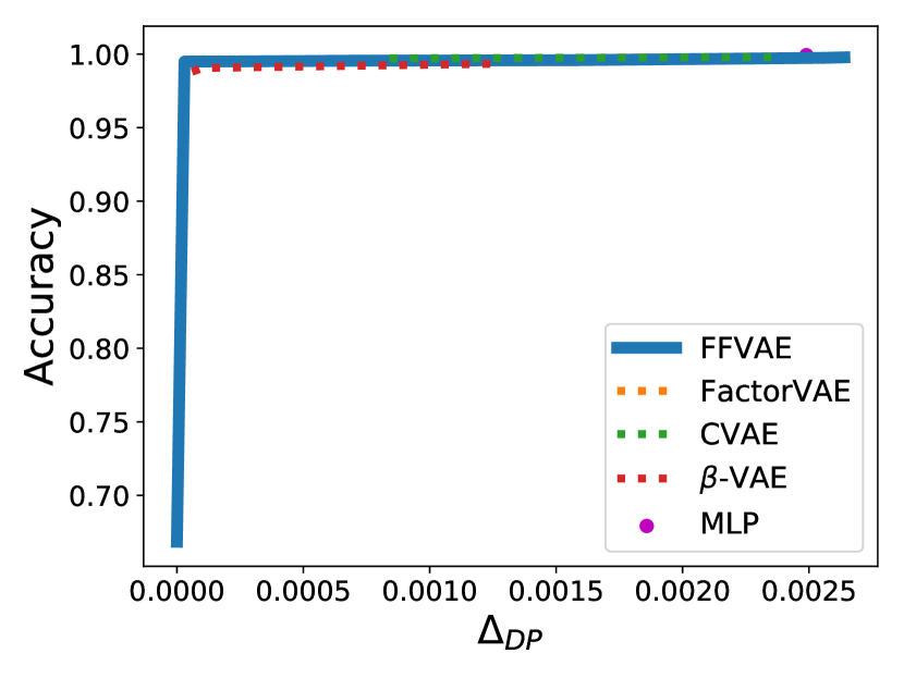
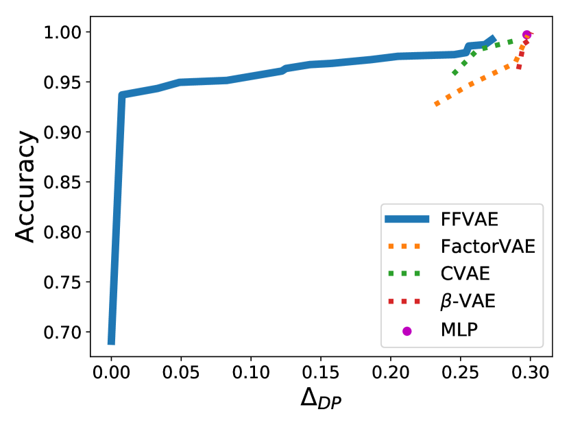
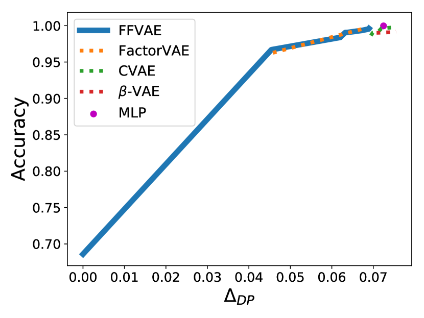
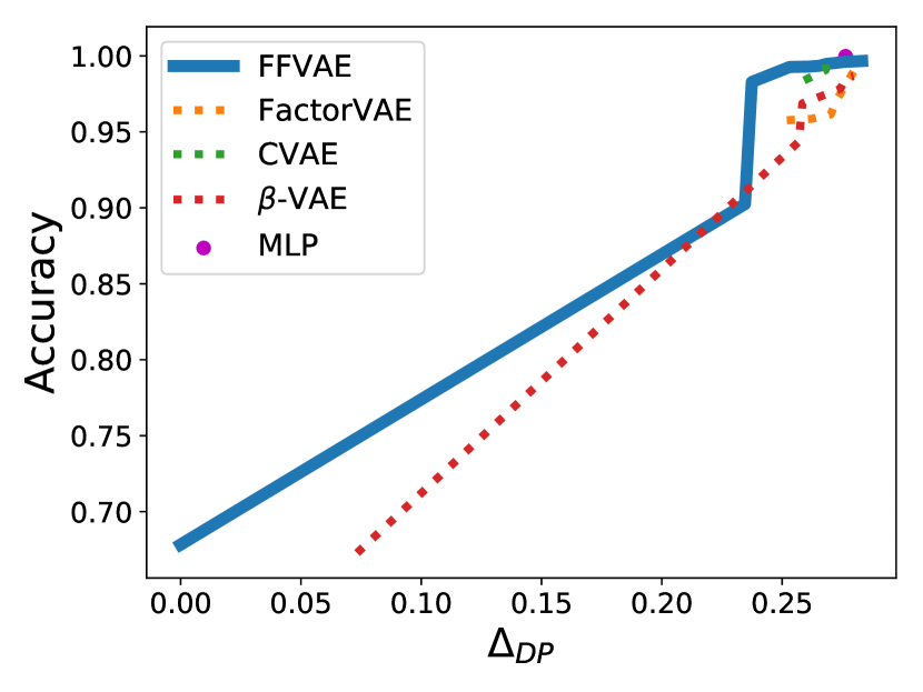
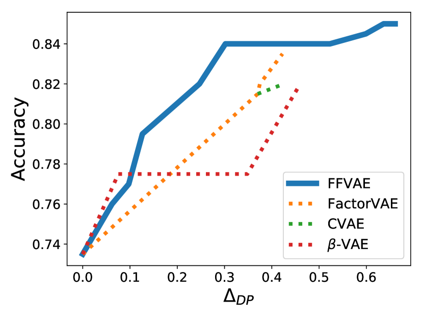
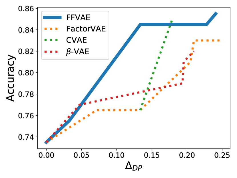
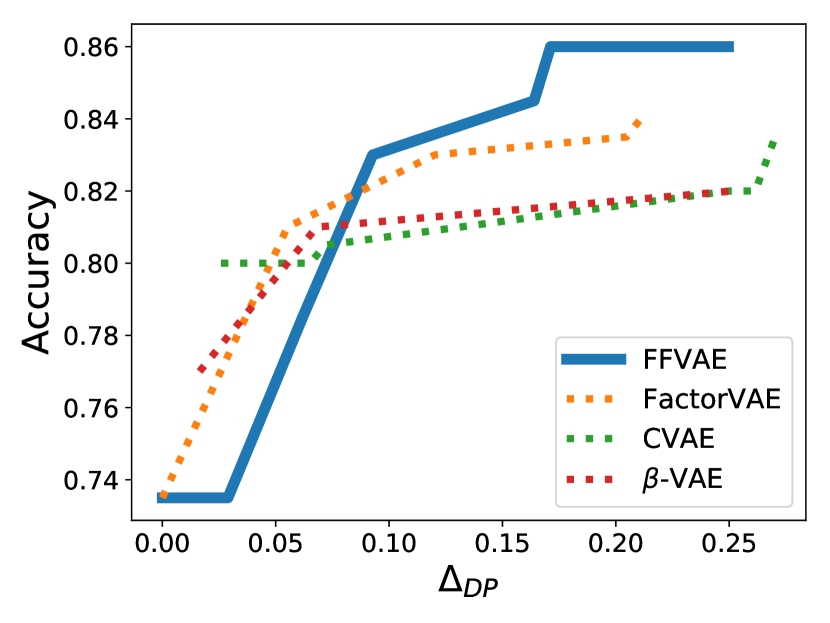
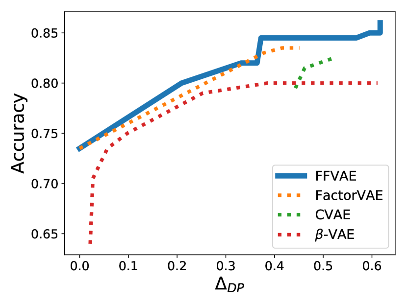
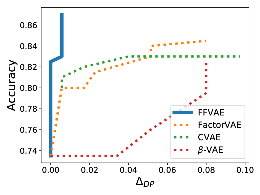
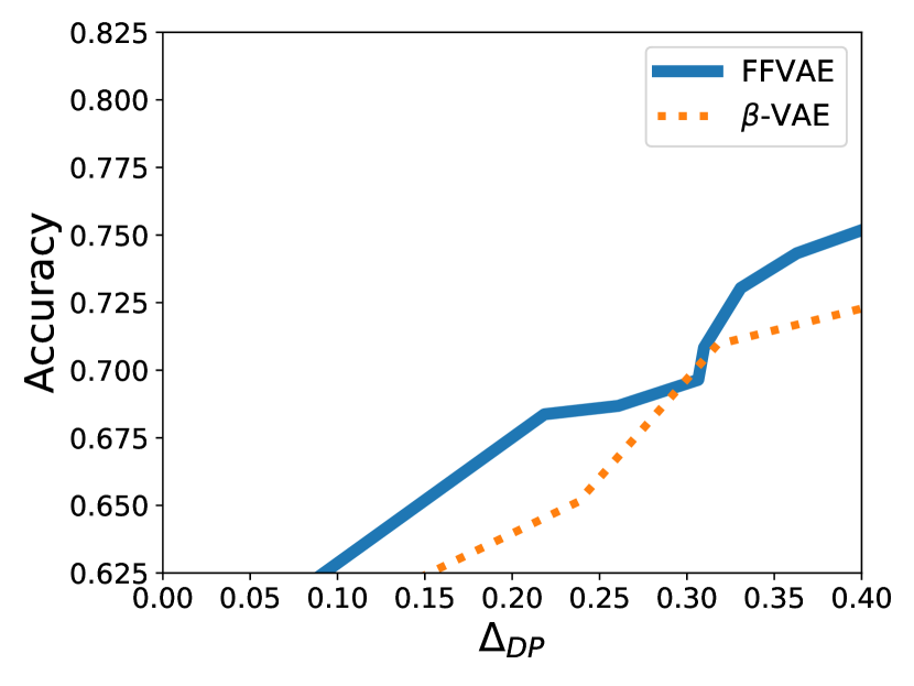
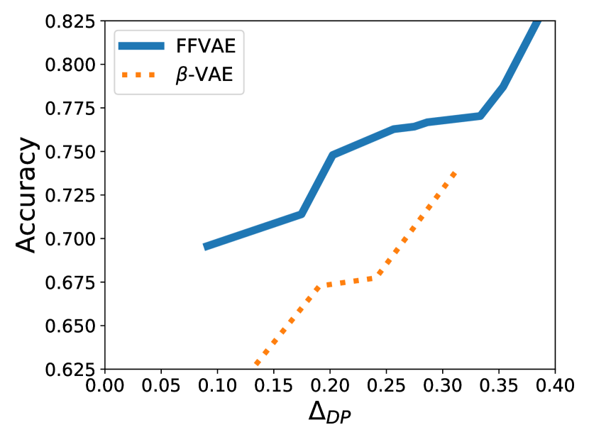
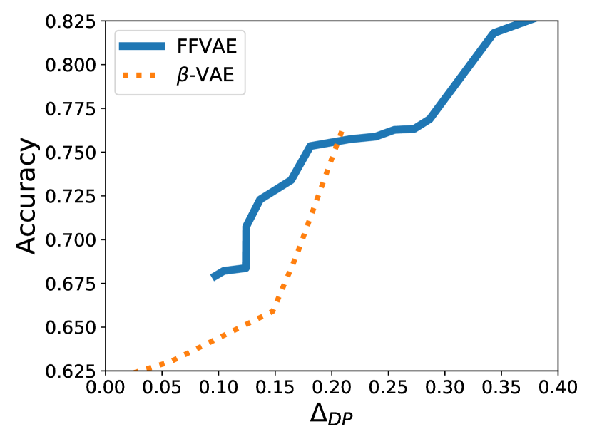
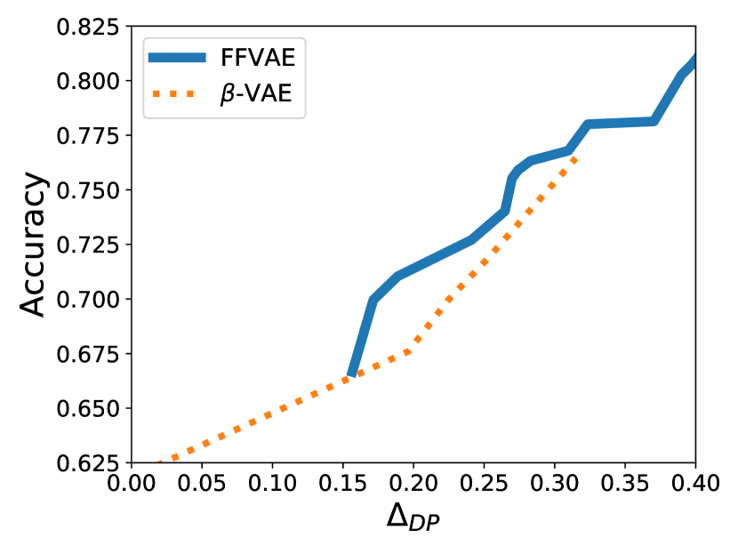
We perform the fair classification audit using several group/subgroup definitions for models trained on DSpritesUnfair (see Appendix D for training details), and report fairness-accuracy tradeoff curves in Fig. 2. In these experiments, we used Shape and Scale as our sensitive attributes during encoder training. We perform the fair classification audit by training an MLP to predict “XPosition”—which was not used in the representation learning phase—given the modified encoder outputs, and repeat for several sensitive groups and subgroups. We modify the encoder outputs as follows: When our sensitive attribute is we remove the associated dimension from ; when the attribute is a conjunction of and , we remove both and . For the baselines, we simply remove the latent dimension which is most correlated with , or the two most correlated dimensions with the conjunction. We sweep a range of hyperparameters to produce the fairness-accuracy tradeoff curve for each model. In Fig. 2, we show the “Pareto front” of these models: points in (, accuracy)-space for which no other point is better along both dimensions. The optimal result is the top left hand corner (perfect accuracy and ).
Since we have a 2-D sensitive input space, we show results for four different sensitive attributes derived from these dimensions: . Recall that Shape and XPosition correlate in the DSpritesUnfair dataset. Therefore, for sensitive attributes that involve Shape, we expect to see an improvement in . For sensitive attributes that do not involve Shape, we expect that our method does not hurt performance at all — since the attributes are uncorrelated in the data, the optimal predictive solution also has .
When group membership is uncorrelated with label (Fig. 2(a)), all models achieve high accuracy and low ( and successfully disentangled). When correlates with by design (Fig. 2(b)), we see the clearest improvement of the FFVAE over the baselines, with an almost complete reduction in and very little accuracy loss. The baseline models are all unable to improve by more than about 0.05, indicating that they have not effectively disentangled the sensitive information from the label. In Figs. 2(c) and 2(d), we examine conjunctions of sensitive attributes, assessing FFVAE’s ability to flexibly provide multi-attribute fair representations. Here FFVAE exceeds or matches the baselines accuracy-at-a-given- almost everywhere; by disentangling information from multiple sensitive attributes, FFVAE enables flexibly fair downstream classification.
Disentanglement and Predictiveness
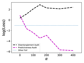
Fig. 3 shows the FFVAE disentanglement and predictiveness audits (see above for description of this procedure). This result aggregates audits across all FFVAE models trained in the setting from Figure 2(b). The classifier loss is cross-entropy, which is a lower bound on the mutual information between the input and target of the classifier. We observe that increasing helps both predictiveness and disentanglement in this scenario. In the disentanglement audit, larger makes predicting the sensitive attribute from the modified representation (with removed) more difficult. The horizontal dotted line shows the log loss of a classifier that predicts from the other DSprites factors of variation (including labels not available to FFVAE); this baseline reflects the correlation inherent in the data. We see that when (i.e. FactorVAE), it is slightly more difficult than this baseline to predict the sensitive attribute. This is due to the disentanglement prior. However, increasing increases disentanglement benefits in FFVAE beyond what is present in FactorVAE. This shows that encouraging predictive structure can help disentanglement through isolating each attribute’s information in particular latent dimensions. Additionally, increasing improves predictiveness, as expected from the objective formulation. We further evaluate the disentanglement properties of our model in Appendix E using the Mutual Information Gap metric (Chen et al., 2018).
5.3 Communities & Crime
Dataset
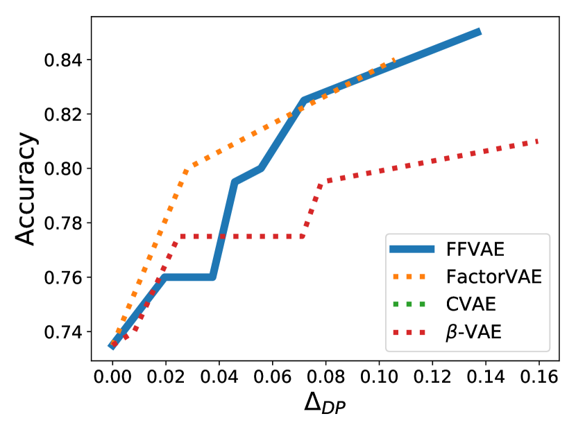
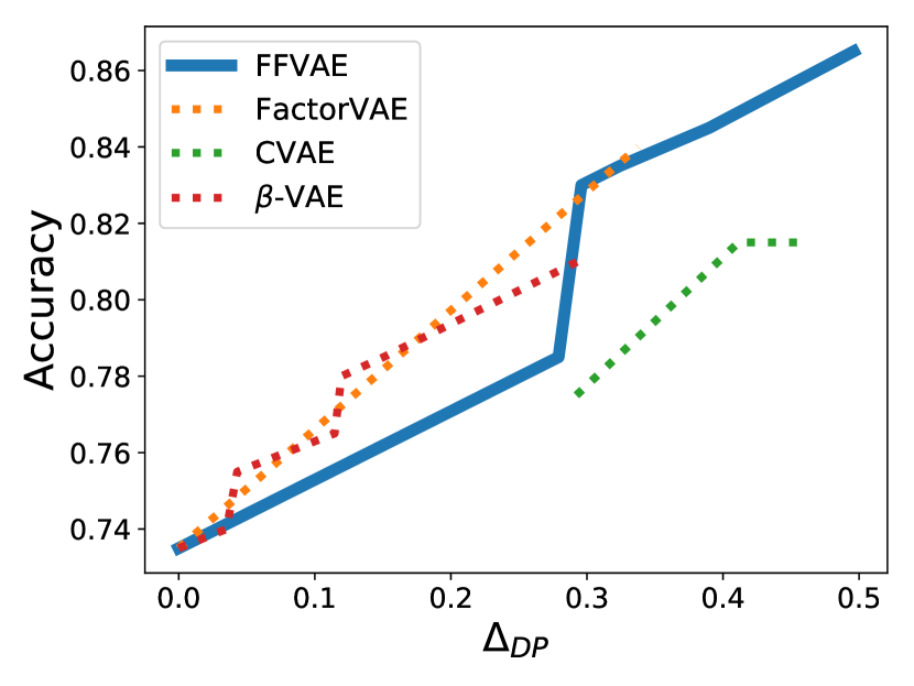
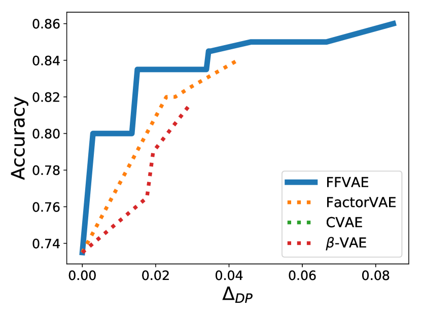
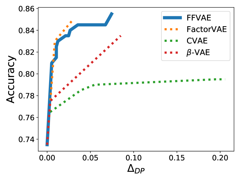
Communities & Crime555http://archive.ics.uci.edu/ml/datasets/communities+and+crime is a tabular UCI dataset containing neighborhood-level population statistics. 120 such statistics are recorded for each of the neighborhoods. Several attributes encode demographic information that may be protected. We chose three as sensitive: racePctBlack (% neighborhood population which is Black), blackPerCap (avg per capita income of Black residents), and pctNotSpeakEnglWell (% neighborhood population that does not speak English well). We follow the same train/eval procedure as with DSpritesUnfair - we train FFVAE with the sensitive attributes and evaluate using naive MLPs to predict a held-out label (violent crimes per capita) on held-out data.
Fair Classification
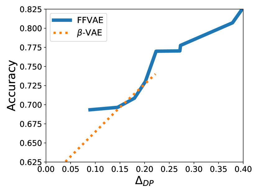
This dataset presents a more difficult disentanglement problem than DSpritesUnfair. The three sensitive attributes we chose in Communities and Crime were somewhat correlated with each other, a natural artefact of using real (rather than simulated) data. We note that in general, the disentanglement literature does not provide much guidance in terms of disentangling correlated attributes. Despite this obstacle, FFVAE performed reasonably well in the fair classification audit (Fig. 4). It achieved higher accuracy than the baselines in general, likely due to its ability to incorporate side information from during training. Among the baselines, FactorVAE tended perform best, suggesting achieving a factorized aggregate posterior helps with fair classification. While our method does not outperform the baselines on each conjunction, its relatively strong performance on a difficult, tabular dataset shows the promise of using disentanglement priors in designing robust subgroup-fair machine learning models.
5.4 Celebrity Faces
Dataset
The CelebA666http://mmlab.ie.cuhk.edu.hk/projects/CelebA.html dataset contains over images of celebrity faces. Each image is associated with 40 human-labeled binary attributes (OvalFace, HeavyMakeup, etc.). We chose three attributes, Chubby, Eyeglasses, and Male as sensitive attributes777 We chose these attributes because they co-vary relatively weakly with each other (compared with other attribute triplets), but strongly with other attributes. Nevertheless the rich correlation structure amongst all attributes makes this a challenging fairness dataset; it is difficult to achieve high accuracy and low . , and report fair classification results on 3 groups and 12 two-attribute-conjunction subgroups only (for brevity we omit three-attribute conjunctions). To our knowledge this is the first exploration of fair representation learning algorithms on the Celeb-A dataset. As in the previous sections we train the encoders on the train set, then evaluate performance of MLP classifiers trained on the encoded test set.
Fair Classification
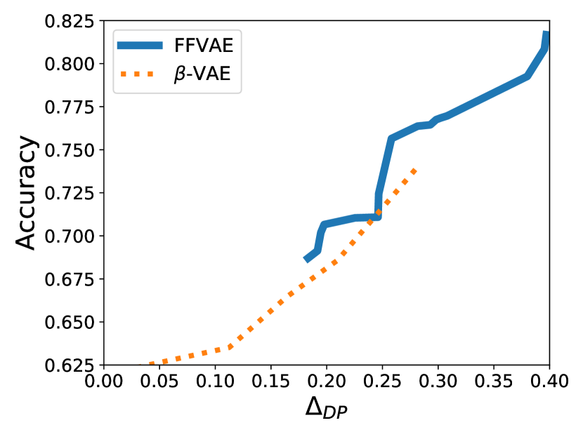
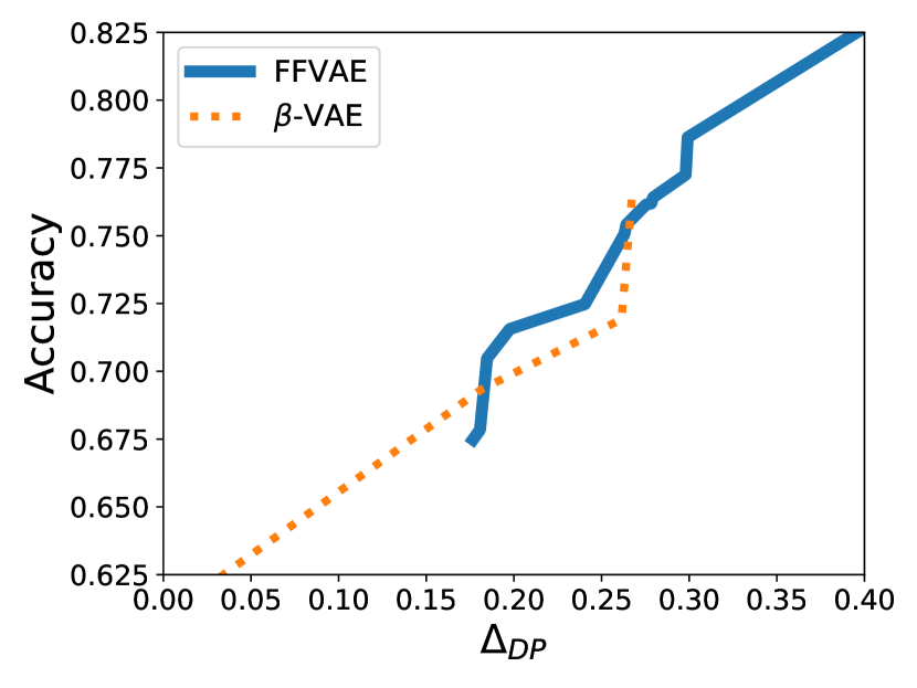
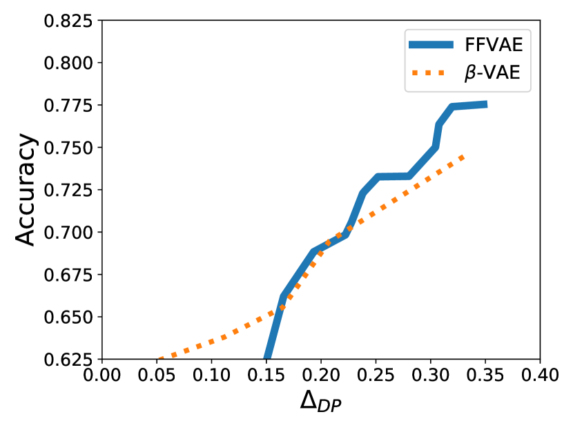
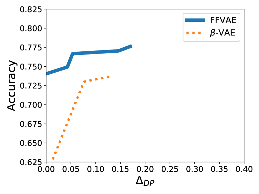
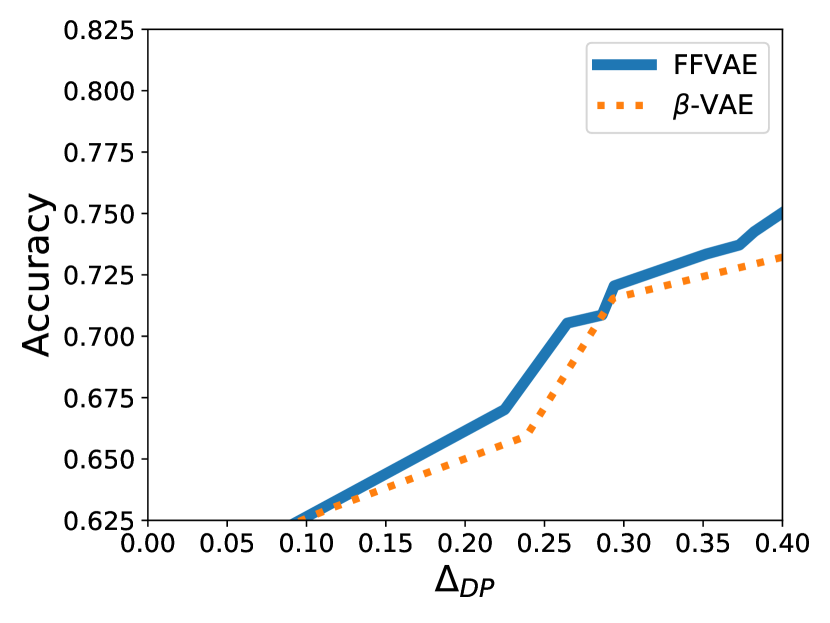
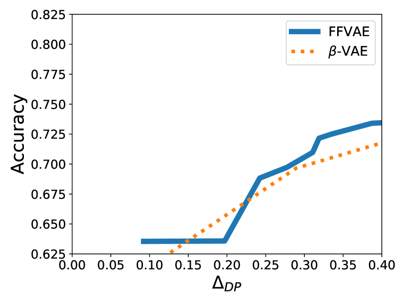
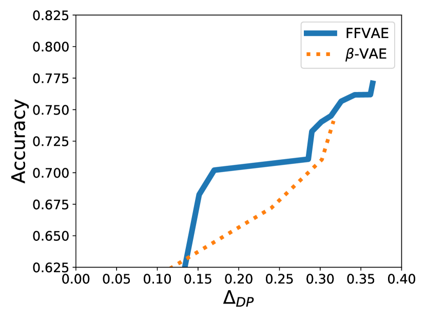
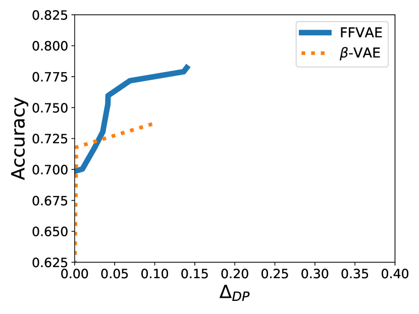
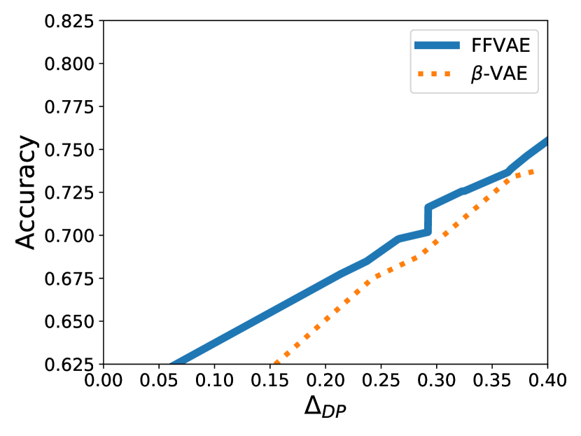
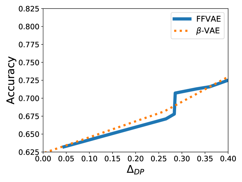
We follow the fair classification audit procedure described above, where the held-out label HeavyMakeup—which was not used at encoder train time—is predicted by an MLP from the encoder representations. When training the MLPs we take a fresh encoder sample for each minibatch (statically encoding the dataset with one encoder sample per image induced overfitting). We found that training the MLPs on encoder means (rather than samples) increased accuracy but at the cost of very unfavorable . We also found that FactorVAE-style adversarial training does not scale well to this high-dimensional problem, so we instead optimize Equation 4 using the biased estimator from Chen et al. (2018). Figure 5 shows Pareto fronts that capture the fairness-accuracy tradeoff for FFVAE and -VAE.
While neither method dominates in this challenging setting, FFVAE achieves a favorable fairness-accuracy tradeoff across many of subgroups. We believe that using sensitive attributes as side information gives FFVAE an advantage over -VAE in predicting the held-out label. In some cases (e.g., =EM) FFVAE achieves better accuracy at all levels, while in others (e.g., =CE) , FFVAE did not find a low- solution. We believe Celeb-A–with its many high dimensional data and rich label correlations—is a useful test bed for subgroup fair machine learning algorithms, and we are encouraged by the reasonably robust performance of FFVAE in our experiments.
6 Discussion
In this paper we discussed how disentangled representation learning aligns with the goals of subgroup fair machine learning, and presented a method for learning a structured latent code using multiple sensitive attributes. The proposed model, FFVAE, provides flexibly fair representations, which can be modified simply and compositionally at test time to yield a fair representation with respect to multiple sensitive attributes and their conjunctions, even when test-time sensitive attribute labels are unavailable. Empirically we found that FFVAE disentangled sensitive sources of variation in synthetic image data, even in the challenging scenario where attributes and labels correlate. Our method compared favorably with baseline disentanglement algorithms on downstream fair classifications by achieving better parity for a given accuracy budget across several group and subgroup definitions. FFVAE also performed well on the Communities & Crime and Celeb-A dataset, although none of the models performed robustly across all possible subgroups in the real-data setting. This result reflects the difficulty of subgroup fair representation learning and motivates further work on this topic.
There are two main directions of interest for future work. First is the question of fairness metrics: a wide range of fairness metrics beyond demographic parity have been proposed (Hardt et al., 2016; Pleiss et al., 2017). Understanding how to learn flexibly fair representations with respect to other metrics is an important step in extending our approach. Secondly, robustness to distributional shift presents an important challenge in the context of both disentanglement and fairness. In disentanglement, we aim to learn independent factors of variation. Most empirical work on evaluating disentanglement has used synthetic data with uniformly distributed factors of variation, but this setting is unrealistic. Meanwhile, in fairness, we hope to learn from potentially biased data distributions, which may suffer from both undersampling and systemic historical discrimination. We might wish to imagine hypothetical “unbiased” data or compute robustly fair representations, but must do so given the data at hand. While learning fair or disentangled representations from real data remains a challenge in practice, we hope that this investigation serves as a first step towards understanding and leveraging the relationship between the two areas.
References
- Alemi et al. (2018) Alemi, A., Poole, B., Fischer, I., Dillon, J., Saurous, R. A., and Murphy, K. Fixing a broken elbo. In Proceedings of the 35th International Conference on Machine Learning, 2018.
- Aleo & Svirsky (2008) Aleo, M. and Svirsky, P. Foreclosure fallout: the banking industry’s attack on disparate impact race discrimination claims under the fair housing act and the equal credit opportunity act. Public Law Interest Journal, 18(1):1–66, 2008. URL https://www.bu.edu/pilj/files/2015/09/18-1AleoandSvirskyArticle.pdf.
- Ardizzone et al. (2019) Ardizzone, L., Kruse, J., Wirkert, S., Rahner, D., Pellegrini, E. W., Klessen, R. S., Maier-Hein, L., Rother, C., and Köthe, U. Analyzing inverse problems with invertible neural networks. In International Conference on Learning Representations, 2019.
- Bach & Jordan (2002) Bach, F. R. and Jordan, M. I. Kernel independent component analysis. Journal of machine learning research, 3(Jul):1–48, 2002.
- Barocas & Selbst (2016) Barocas, S. and Selbst, A. D. Big data’s disparate impact. Calif. L. Rev., 104:671, 2016.
- Bose & Hamilton (2018) Bose, A. J. and Hamilton, W. L. Compositional fairness constraints for graph embeddings. Relational Representation Learning Workshop, Neural Information Processing Systems 2018, 2018.
- Botros & Tomczak (2018) Botros, P. and Tomczak, J. M. Hierarchical vampprior variational fair auto-encoder. In ICML 2018 Workshop on Theoretical Foundations and Applications of Deep Generative Models, 2018.
- Buolamwini & Gebru (2018) Buolamwini, J. and Gebru, T. Gender shades: Intersectional accuracy disparities in commercial gender classification. In Conference on Fairness, Accountability and Transparency, pp. 77–91, 2018.
- Burgess et al. (2017) Burgess, C. P., Higgins, I., Pal, A., Matthey, L., Watters, N., Desjardins, G., and Lerchner, A. Understanding disentangling in -VAE. In 2017 NIPS Workshop on Learning Disentangled Representations, 2017.
- Chen et al. (2018) Chen, T. Q., Li, X., Grosse, R. B., and Duvenaud, D. K. Isolating sources of disentanglement in variational autoencoders. In Advances in Neural Information Processing Systems, pp. 2610–2620, 2018.
- Comon (1994) Comon, P. Independent component analysis, a new concept? Signal processing, 36(3):287–314, 1994.
- DCCA (1983) DCCA. Division of consumer and community affairs. 2011-07. 12 cfr supplement i to part 202 - official staff interpretations. https://www.law.cornell.edu/cfr/text/12/appendix-Supplement_I_to_part_202, 1983.
- Edwards & Storkey (2016) Edwards, H. and Storkey, A. Censoring representations with an adversary. In International Conference on Learning Representations, 2016.
- Elliot et al. (2008) Elliot, M. N., Fremont, A., Morrison, P. A., Pantoja, P., and Lurie, N. A New Method for Estimating Race/Ethnicity and Associated Disparities Where Administrative Records Lack Self‐Reported Race/Ethnicity. Health Services Research, 2008.
- Esmaeili et al. (2019) Esmaeili, B., Wu, H., Jain, S., Bozkurt, A., Siddharth, N., Paige, B., Brooks, D. H., Dy, J., and van de Meent, J.-W. Structured disentangled representations. In The 22nd International Conference on Artificial Intelligence and Statistics, 2019.
- Hardt et al. (2016) Hardt, M., Price, E., Srebro, N., et al. Equality of opportunity in supervised learning. In Advances in neural information processing systems, pp. 3315–3323, 2016.
- Hebert-Johnson et al. (2018) Hebert-Johnson, U., Kim, M., Reingold, O., and Rothblum, G. Multicalibration: Calibration for the (Computationally-identifiable) masses. In Proceedings of the 35th International Conference on Machine Learning, 2018.
- Hellman (2018) Hellman, D. Indirect discrimination and the duty to avoid compounding injustice. Foundations of Indirect Discrimination Law, 2018.
- Higgins et al. (2017) Higgins, I., Matthey, L., Pal, A., Burgess, C., Glorot, X., Botvinick, M., Mohamed, S., and Lerchner, A. In International Conference on Learning Representations, 2017.
- Hyvärinen & Oja (2000) Hyvärinen, A. and Oja, E. Independent component analysis: algorithms and applications. Neural networks, 13(4-5):411–430, 2000.
- Jacobsen et al. (2019) Jacobsen, J.-H., Behrmann, J., Zemel, R., and Bethge, M. Excessive invariance causes adversarial vulnerability. In International Conference on Learning Representations, 2019.
- Kearns et al. (2018) Kearns, M., Neel, S., Roth, A., and Wu, Z. S. Preventing fairness gerrymandering: Auditing and learning for subgroup fairness. In Proceedings of the 35th International Conference on Machine Learning, 2018.
- Kearns et al. (2019) Kearns, M. J., Neel, S., Roth, A., and Wu, Z. S. An empirical study of rich subgroup fairness for machine learning. In Conference on Fairness, Accountability and Transparency, 2019.
- Kim & Mnih (2018) Kim, H. and Mnih, A. Disentangling by factorising. In Proceedings of the 35th International Conference on Machine Learning, 2018.
- Kim et al. (2019) Kim, M. P., Ghorbani, A., and Zou, J. Multiaccuracy: Black-box post-processing for fairness in classification. In AAAI Conference on AI, Ethics, and Society, 2019.
- Kim et al. (2015) Kim, S.-E., Paik, H. Y., Yoon, H., Lee, J. E., Kim, N., and Sung, M.-K. Sex- and gender-specific disparities in colorectal cancer risk. World Journal of Gastroentorology, 21(17):5167–5175, 2015.
- Kingma & Ba (2015) Kingma, D. and Ba, J. Adam: A method for stochastic optimization. In International Conference on Learning Representations, 2015.
- Kingma & Welling (2013) Kingma, D. P. and Welling, M. Auto-encoding variational bayes. arXiv preprint arXiv:1312.6114, 2013.
- Kingma et al. (2014) Kingma, D. P., Mohamed, S., Rezende, D. J., and Welling, M. Semi-supervised learning with deep generative models. In Advances in neural information processing systems, pp. 3581–3589, 2014.
- Kirchner et al. (2016) Kirchner, L., Mattu, S., Larson, J., and Angwin, J. Machine Bias: There’s Software Used Across the Country to Predict Future Criminals. And it’s Biased Against Blacks., May 2016. URL https://www.propublica.org/article/machine-bias-risk-assessments-in-criminal-sentencing.
- Klys et al. (2018) Klys, J., Snell, J., and Zemel, R. Learning latent subspaces in variational autoencoders. In Advances in Neural Information Processing Systems, pp. 6443–6453, 2018.
- Kusner et al. (2017) Kusner, M. J., Loftus, J., Russell, C., and Silva, R. Counterfactual fairness. In Advances in Neural Information Processing Systems 30. 2017.
- Locatello et al. (2019) Locatello, F., Bauer, S., Lucic, M., Gelly, S., Schölkopf, B., and Bachem, O. Challenging common assumptions in the unsupervised learning of disentangled representations. In Proceedings of the 36th International Conference on Machine Learning, 2019.
- Louizos et al. (2016) Louizos, C., Swersky, K., Li, Y., Welling, M., and Zemel, R. The variational fair autoencoder. In International Conference on Learning Representations, 2016.
- Madras et al. (2018) Madras, D., Creager, E., Pitassi, T., and Zemel, R. Learning adversarially fair and transferable representations. In Proceedings of the 35th International Conference on Machine Learning, 2018.
- Moyer et al. (2018) Moyer, D., Gao, S., Brekelmans, R., Galstyan, A., and Ver Steeg, G. Invariant representations without adversarial training. In Advances in Neural Information Processing Systems, pp. 9101–9110, 2018.
- Pleiss et al. (2017) Pleiss, G., Raghavan, M., Wu, F., Kleinberg, J., and Weinberger, K. Q. On fairness and calibration. In Advances in Neural Information Processing Systems. 2017.
- Rothenhäusler et al. (2018) Rothenhäusler, D., Meinshausen, N., Bühlmann, P., and Peters, J. Anchor regression: heterogeneous data meets causality. arXiv preprint arXiv:1801.06229, 2018.
- Song et al. (2019) Song, J., Kalluri, P., Grover, A., Zhao, S., and Ermon, S. Learning controllable fair representations. In The 22nd International Conference on Artificial Intelligence and Statistics, 2019.
- Zemel et al. (2013) Zemel, R., Wu, Y., Swersky, K., Pitassi, T., and Dwork, C. Learning fair representations. In Proceedings of the 30th International Conference on Machine Learning, 2013.
Appendix A Discriminator approximation of total correlation
This section describes how density ratio estimation is implemented to train the FFVAE encoder. We follow the approach of Kim & Mnih (2018).
Generating Samples
The binary classifier adversary seeks to discriminate between
-
•
, “true” samples from the aggregate posterior; and
-
•
, “fake” samples from the product of the marginal over and the marginals over each .
At train time, after splitting the latent code of the -example along the dimensions of as , the minibatch index order for each subspace is then randomized, simulating samples from the product of the marginals; these dimension-shuffled samples retain the same marginal statistics as “real” (unshuffled) samples, but with joint statistics between the subspaces broken. The overall minibatch of encoder outputs contains twice as many examples as the original image minibatch, and comprises equal number of “real” and “fake” samples.
As we describe below, the encoder output minibatch is used as training data for the adversary, and the error is backpropagated to the encoder weights so the encoder can better fool the adversary. If a strong adversary can do no better than random chance, then the desired independence property has been achieved.
Discriminator Approximation
Here we summarize the the approximation of the term from equation 4. Let be an indicator variable with indicating comes from a minibatch of “real” encoder distributions, while indicating is drawn from a “fake” minibatch of shuffled samples, i.e., is drawn from the product of the marginals of the aggregate posterior. The discriminator network outputs the probability that vector is a “real” sample, i.e., where is the discriminator and is the sigmoid function. If the discriminator is well-trained to distinguish between “real” and “fake” samples then we have
| (5) | ||||
We can substitute this into the KL divergence as
| (6) |
Meanwhile the discriminator is trained by minimizing the standard cross entropy loss
| (7) |
w.r.t. the parameters of . This ensures that the discriminator output is a calibrated approximation of the log density .
and (Equation 4) are then optimized in a min-max fashion. In our experiments we found that single-step alternating updates using optimizers with the same settings sufficed for stable optimization.
Appendix B DSpritesUnfair Generation
The original DSprites dataset has six ground truth factors of variation (FOV):
-
•
Color: white
-
•
Shape: square, ellipse, heart
-
•
Scale: 6 values linearly spaced in
-
•
Orientation: 40 values in
-
•
XPosition: 32 values in
-
•
YPosition: 32 values in
In the original dataset the joint distribution over all FOV factorized; each FOV was considered independent. In our dataset, we instead sample such that the FOVs Shape and X-position correlate. We associate an index with each possible value of each attribute, and then sample a (Shape, X-position) pair with probability proportional to , where are the indices, total number of options, and a real number for each of Shape and X-position ( respectively). We use . All other attributes are sampled uniformly, as in the standard version of DSprites.
We binarized the factors of variation by using the boolean outputs of the following operations:
-
•
Color
-
•
Shape
-
•
Scale
-
•
Rotation
-
•
XPosition
-
•
YPosition
Appendix C DSprites Architectures
The architectures for the convolutional encoder , decoder , and FFVAE discriminator are specified as follows.
import torch
from torch import nn
class Resize(torch.nn.Module):
def __init__(self, size):
super(Resize, self).__init__()
self.size = size
def forward(self, tensor):
return tensor.view(self.size)
class ConvEncoder(nn.Module):
def __init__(self, im_shape=[64, 64], latent_dim=10, n_chan=1):
super(ConvEncoder, self).__init__()
self.f = nn.Sequential(
Resize((-1,n_chan,im_shape[0],im_shape[1])),
nn.Conv2d(n_chan, 32, 4, 2, 1),
nn.ReLU(True),
nn.Conv2d(32, 32, 4, 2, 1),
nn.ReLU(True),
nn.Conv2d(32, 64, 4, 2, 1),
nn.ReLU(True),
nn.Conv2d(64, 64, 4, 2, 1),
nn.ReLU(True),
Resize((-1,1024)),
nn.Linear(1024, 128),
nn.ReLU(True),
nn.Linear(128, 2*latent_dim)
)
self.im_shape = im_shape
self.latent_dim = latent_dim
def forward(self, x):
mu_and_logvar = self.f(x)
mu = mu_and_logvar[:, :self.latent_dim]
logvar = mu_and_logvar[:, self.latent_dim:]
return mu, logvar
class ConvDecoder(nn.Module):
def __init__(self, im_shape=[64, 64], latent_dim=10, n_chan=1):
super(ConvDecoder, self).__init__()
self.g = nn.Sequential(
nn.Linear(latent_dim, 128),
nn.ReLU(True),
nn.Linear(128, 1024),
nn.ReLU(True),
Resize((-1,64,4,4)),
nn.ConvTranspose2d(64, 64, 4, 2, 1),
nn.ReLU(True),
nn.ConvTranspose2d(64, 32, 4, 2, 1),
nn.ReLU(True),
nn.ConvTranspose2d(32, 32, 4, 2, 1),
nn.ReLU(True),
nn.ConvTranspose2d(32, n_chan, 4, 2, 1),
)
def forward(self, z):
x = self.g(z)
return x.squeeze()
class Discriminator(nn.Module):
def __init__(self, n):
super(Discriminator, self).__init__()
self.model = nn.Sequential(
nn.Linear(n, 1000),
nn.LeakyReLU(0.2, inplace=True),
nn.Linear(1000, 1000),
nn.LeakyReLU(0.2, inplace=True),
nn.Linear(1000, 1000),
nn.LeakyReLU(0.2, inplace=True),
nn.Linear(1000, 1000),
nn.LeakyReLU(0.2, inplace=True),
nn.Linear(1000, 1000),
nn.LeakyReLU(0.2, inplace=True),
nn.Linear(1000, 2),
)
selftmax = nn.Softmax(dim=1)
def forward(self, zb):
logits = self.model(zb)
probs = nn.Softmax(dim=1)(logits)
return logits, probs
Appendix D DSpritesUnfair Training Details
All network parameters were optimized using the Adam (Kingma & Ba, 2015), with learning rate 0.001. Architectures are specified in Appendix C. Our encoders trained iterations with minibatch size 64 (as in Kim & Mnih (2018)). Our MLP classifier has two hidden layers with 128 units each, and is trained with patience of 5 epochs on validation loss.
Appendix E Mutual Information Gap
Evaluation Criteria
Here we analyze the encoder mutual information in the synthetic setting of the DSpritesUnfair dataset, where we know the ground truth factors of variation. In Fig. 6, we calculate the Mutual Information Gap (MIG) (Chen et al., 2018) of FFVAE across various hyperparameter settings. With latent variables and factors of variation , MIG is defined as
| (8) |
where , denotes mutual information, and is the number of factors of variation. Note that we can only compute this metric in the synthetic setting where the ground truth factors of variation are known. MIG measures the difference between the latent variables which have the highest and second-highest with each factor of variation, rewarding models which allocate one latent variable to each factor of variation. We test our disentanglement by training our models on a biased version of DSprites, and testing on a balanced version (similar to the “skewed” data in Chen et al. (2018)). This allows us to separate out two sources of correlation — the correlation existing across the data, and the correlation in the model’s learned representation.
Results
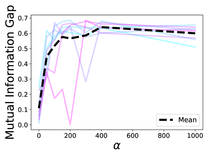
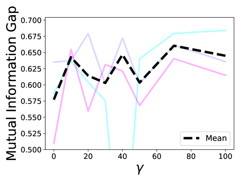
In Fig. 6(a), we show that MIG increases with , providing more evidence that the supervised structure of the FFVAE can create disentanglement. This improvement holds across values of , except for some training instability for the highest values of . It is harder to assess the relationship between and MIG, due to increased instability in training when is large and is small. However, in Fig. 6(b), we look only at , and note that in this range, MIG improves as increases. See Appendix E for more details.
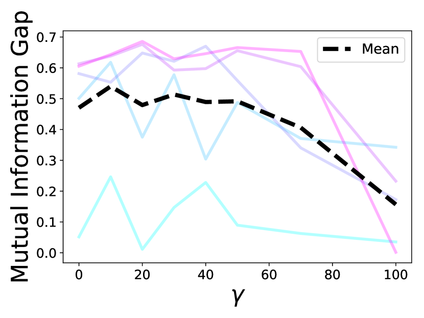
In Fig. 7(a), we show that for low values of , increasing leads to worse MIG, likely due to increased training instability. This is in contrast to Fig. 6(b), which suggests that for high enough , increasing can improve MIG. This leads us to believe that and have a complex relationship with respect to disentanglement and MIG.
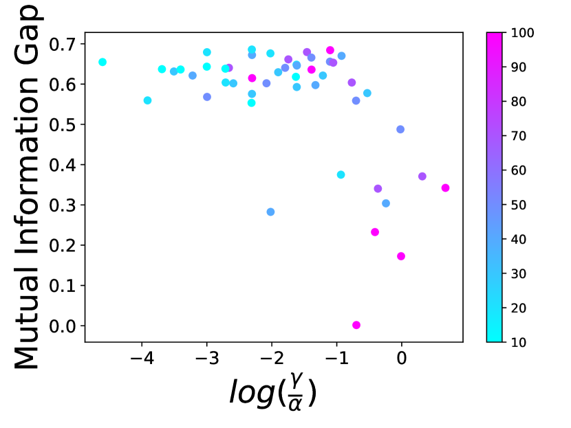
To better understand the relationship between these two hyperparameters, we examine how MIG varies with the ratio in Fig. 7(b). In We find that in general, a higher ratio yields lower MIG, but that the highest MIGs are around , with a slight tailing off for smaller ratios. This indicates there is a dependent relationship between the values of and .
Discussion
What does it mean for our model to demonstrate disentanglement on test data drawn from a new distribution? For interpretation, we can look to the causal inference literature, where one goal is to produce models that are robust to certain interventions in the data generating process (Rothenhäusler et al., 2018). We can interpret Figure 6 as evidence that our learned representations are (at least partially) invariant to interventions on . This property relates to counterfactual fairness, which requires that models be robust with respect to counterfactuals along (Kusner et al., 2017).