Estimation and Tracking of a Moving Target by Unmanned Aerial Vehicles

Abstract

An image-based control strategy along with estimation of target motion is developed to track dynamic targets without motion constraints. To the best of our knowledge, this is the first work that utilizes a bounding box as image features for tracking control and estimation of dynamic target without motion constraint. The features generated from a You-Only-Look-Once (YOLO) deep neural network can relax the assumption of continuous availability of the feature points in most literature and minimize the gap for applications. The challenges are that the motion pattern of the target is unknown and modeling its dynamics is infeasible. To resolve these issues, the dynamics of the target is modeled by a constant-velocity model and is employed as a process model in the Unscented Kalman Filter (UKF), but process noise is uncertain and sensitive to system instability. To ensure convergence of the estimate error, the noise covariance matrix is estimated according to history data within a moving window. The estimated motion from the UKF is implemented as a feedforward term in the developed controller, so that tracking performance is enhanced. Simulations are demonstrated to verify the efficacy of the developed estimator and controller.

I Introduction

Knowledge about the position and velocity of surrounding objects is important to the booming fields such as self-driving cars, target tracking and monitoring. In case of performing an object tracking task, position and velocity of the tracking target are typically assumed to be available to achieve better control performance [1] and [2] using visual servo controllers. When the target is not static, its velocity needs be considered in the system dynamics as to eliminate the tracking error and to calculate the accurate motion command for the camera. However, obtaining the knowledge online is challenging since the dynamics of the target might be complicated and unknown. Moreover, there are instances that the measurement can be unexpected. For example, the target can exceed the field of view (FOV) of the camera, or cannot be detected due to the unexpected occlusion. Several approaches have been proposed for estimating position or velocity of the target such as by using a fixed camera[3], sensor networks [4, 5, 6], radar [7], and some known reference information in the image scene[8]. In order to integrate with applications based on vision system such as target tracking, exploration, visual servo control and navigation [1] and [9, 10, 11], an algorithm for a monocular camera to estimate position and velocity of a moving target is developed in this work.

To continuously estimate the position or the velocity of a target, it needs to remain in the field of view of the camera, and therefore, motion of the target should be considered. Structure from motion (SfM), Structure and Motion (SaM) methods are usually used to reconstruct the relative position and motion between the vision system and objects in many applications [1] and [2]. With the knowledge of length between two feature points, [12] proposed methods to estimate position of the stationary features. In [13], 3D Euclidean structure of a static object is estimated based on the linear and angular velocities of a single camera mounted on a mobile platform, where the assumption is relaxed in [14]. However, SfM can only estimate the position of the object and usually the object is assumed to be stationary. In order to address the problem to estimate motion of moving objects, SaM is applied for estimation by using the knowledge of camera motion. Nonlinear observers are proposed in [15] and [16] to estimate the structure of a moving object with time-varying velocities. The velocity of the object in [15] is assumed to be constant, and [16] relaxes the constant-velocity assumption to time-varying velocities for targets moving in a straight line or on a ground plane. In practice, measurement can be intermittent when the object is occluded, outside the camera FOV, etc. [17, 18, 19] present the development of dwell time conditions to guarantee that the state estimate error converges to an ultimate bound under intermittent measurement. In [17, 18, 19], the estimation is based on the knowledge about the velocity of the moving object and the camera. However, in practice the velocity of the target is usually unknown, and modeling its dynamics is complicated and challenging.

In fact, the relationship between target motion estimator and vision-based controller is inseparable. Specifically, output from a high performance target motion estimator can be used as a feedforward term for the controller to keep the target in the field of view longer, which, in return, results in a longer period for the estimate error to converge. In this work, a dynamic monocular camera is employed to estimate the position and velocity of a moving target. Compared to the multi-camera system[20], using a monocular camera has the advantage of reducing power consumption and the quantity of image data. A You-Only-Look-Once (YOLO) deep neural network[21] is applied in this work for target detection, which relaxes the assumption of continuous availability of the feature point and minimizes the gap for applications, but it also introduces some challenges. That is, the detected box enclosing the target can lead to intermittent measurement, and the probability distribution function of the noise from inaccurate motion model may not follow the normal distribution. An Unscented Kalman Filter (UKF) based algorithm is developed in this work to deal with problems of intermittent measurement and to obtain continuous estimate the target motion even when it leaves the FOV. To deal with the uncertain noise during the estimation, method in [22] is applied to update the process noise covariance matrix online to guarantee the convergence and the accuracy of the estimation.

II Preliminaries and Problem Statement

II-A Kinematics Model

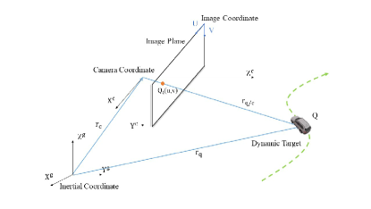
Figure 1: Kinematics model.

Based on the model in [19], Fig. 1 depicts the relationship between a moving target, a camera, and an image plane. The camera is mounted on the multirotor without relative motion. The subscript $\mathcal{G}$ denotes the inertial frame with its origin set arbitrarily on the ground, and the subscript $C$ represents the body-fixed camera frame with its origin fixed at the principle point of the camera, where $Z^{c}$ and $X^{c}$ are axes with denoted direction. The vectors $r_{q}=\left[\begin{array}[]{ccc}x_{q}&y_{q}&z_{q}\end{array}\right]^{T}$ denotes the position of the feature point of the target, which is unknown and to be estimated, $r_{c}=\left[\begin{array}[]{ccc}x_{c}&y_{c}&z_{c}\end{array}\right]^{T}$ denotes the position of the camera, which can be measured by the embedded GPS/Motion Capture Systems, and $r_{q/c}=\left[\begin{array}[]{ccc}X&Y&Z\end{array}\right]^{T}$ denotes the relative position between the feature point and the camera, all expressed in the camera frame. Their relation can be written as

$$r_{q/c} = r_{q}-r_{c}.$$ (1)

Taking the time derivative on the both sides of (1) yields the relative velocity as

$$\dot{r}_{q/c} = V_{q}-V_{c}-\omega_{c}\times r_{q/c},$$ (2)

where $V_{c}\triangleq\left[\begin{array}[]{ccc}v_{cx}&v_{cy}&v_{cz}\end{array}\right]^{T}$ is the linear velocity of the camera, $\omega_{c}\triangleq\left[\begin{array}[]{ccc}\omega_{cx}&\omega_{cy}&\omega_{cz}\end{array}\right]^{T}$ is the angular velocity of the camera, both are the control command to be designed. In (2), $V_{q}=\left[\begin{array}[]{ccc}v_{qx}&v_{qy}&v_{qz}\end{array}\right]^{T}$ is the linear velocity of the dynamic target, which is unknown and needs to be estimated. To relax the limitation of existing results, following assumption is made throughout this work.

Assumption 1.

The trajectory of the target is unknown but bounded.

Since the dynamics of the camera and the target are coupled, the states of the overall system are defined as

$$\mathbf{x}=\left[\begin{array}[]{ccccccccc}x_{1}&x_{2}&x_{3}&x_{q}&y_{q}&z_{q}&v_{qx}&v_{qy}&v_{qz}\end{array}\right]^{T}.$$ (3)

To estimate the position and velocity of the target, the state $\left[\begin{array}[]{ccc}x_{1}&x_{2}&x_{3}\end{array}\right]^{T}=\left[\begin{array}[]{ccc}\frac{X}{Z}&\frac{Y}{Z}&\frac{1}{Z}\end{array}\right]^{T}$ is defined to facilitate the subsequent analysis. Taking the time derivative on the both sides of (3) and using (2) obtain a nonlinear function that represents the dynamics of the overall system as

$$\dot{\mathbf{x}} = \left[\begin{array}[]{c}v_{qx}x_{3}-v_{qz}x_{1}x_{3}+\zeta_{1}+\eta_{1}\\ v_{qy}x_{3}-v_{qz}x_{2}x_{3}+\zeta_{2}+\eta_{2}\\ -v_{qz}x_{3}^{2}+v_{cz}x_{3}^{2}-(\omega_{cy}x_{1}-\omega_{cx}x_{2})x_{3}\\ V_{q}\\ \begin{array}[]{c}0\\ 0\\ 0\end{array}\end{array}\right],$$ (12)

where $\zeta_{1}$, $\zeta_{2}$, $\eta_{1}$, $\eta_{2}\in\mathbb{R}$ are defined as

$$\zeta_{1} =\omega_{cz}x_{2}-\omega_{cy}-\omega_{cy}x_{1}^{2}+\omega_{cx}x_{1}x_{2}$$

$$\zeta_{2} =-\omega_{cz}x_{1}+\omega_{cx}+\omega_{cx}x_{2}^{2}-\omega_{cy}x_{1}x_{2}$$

$$\eta_{1} =(v_{cz}x_{1}-v_{cx})x_{3}$$

$$\eta_{2} =(v_{cz}x_{2}-v_{cy})x_{3}.$$ (13)

Remark 1.

Since the trajectory and motion pattern of the target is unknown, it is modeled by a zero acceleration (i.e., constant velocity) dynamics as formulated in (12), which is reasonable during a short sampling time with the unneglectable mass of the moving target. The mismatch between the true and modeled dynamics can be considered as a process noise in an UKF developed in the subsequent section.

II-B Image Model

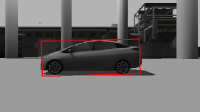
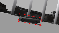
Figure 2: The images of the dynamic targets are captured from an onboard camera on the multirotor in the Gazebo simulator. Note that the center of the bounding box is considered as a feature point for the subsequent analysis, and the bounding boxes, enclosing the vehicles from different angles of inclination, are obtained from a YOLO network that is trained for this work.

By projecting the feature point $Q$ into the image frame using the pinhole model yields the projection point $q=\left[\begin{array}[]{cc}x_{1}&x_{2}\end{array}\right]^{T}\in\mathbb{R}^{2}$ as

$$\begin{array}[]{c}x_{1}=\frac{u-c_{u}}{f_{x}}\\ x_{2}=\frac{v-c_{v}}{f_{y}},\end{array}$$ (14)

where $[u,\,v]^{T}$ denotes the position of the feature point in the image frame, $f_{x}$ and $f_{y}$ are the focal length of pixel unit, and $[c_{u},\,c_{v}]^{T}$ represents the position of the center of the image. The area of the bounding box is defined as $a$ , and based on the pinhole model the relation between $a$ and $x_{3}$ can be expressed as

$$a = Af_{x}f_{y}x_{3}^{2}$$ (15)

where $A$ is the area of the target on the side, observed from the camera.

Assumption 2.

The optical axis of the camera remains perpendicular to $A$ to ensure better detection accuracy from YOLO.

Remark 2.

To estimate $x_{3}$ precisely from (15), $A$ needs to be accurate. Since $A$ is a fixed value, the optical axis of the camera needs to remain at fixed angle relative to the plane of $A.$

II-C Measurement Model

To correct the unobserved system states, the measurement is defined as

$$\mathbf{z}=\left[\begin{array}[]{cccc}u&v&a&r_{c}\end{array}\right]^{T},$$

where $u$, $v$ and $a$ can be obtained directly from the detected bounding box, and $r_{c}$ is measurable as described in Section II-A. By using (1), (14), and (15), the estimate measurement $\hat{\mathbf{z}}$ for the UKF can be obtained as

$$\hat{\mathbf{z}}=\left[\begin{array}[]{c}f_{x}\hat{x}_{1}+c_{u}\\ f_{y}\hat{x}_{2}+c_{v}\\ Af_{x}f_{y}\hat{x}_{3}^{2}\text{sgn}(\hat{x}_{3})\\ \hat{r}_{q}-\hat{r}_{q/c}\end{array}\right]$$ (16)

where $\text{sgn}(\cdotp)$ is a signum function, and $\hat{\left(\cdot\right)}$ is the estimate of the denoted argument obtained from the process step in the UKF developed in the next section. In (15), the area of bounding box $a$ remains positive despite of the sign of $x_{3},$ which is positive since the depth is nonnegative. Therefore, to ensure $\hat{x}_{3}$ converge to a positive value, the term $\text{sgn}(\hat{x}_{3})$ is added to (16).

Remark 3.

Despite the aforementioned advantages, bounding boxes can lose unexpectedly, or the Intersection over Union (IoU) may sometime decrease, leading to intermittent or inaccurate measurements. These inherited defects from the data-driven-based detection motivate the need of Kalman filter for estimation. As the target velocity changes, state predicted by the constant-velocity dynamics model can be inaccurate, and the prediction error can considered as process noise.

III Position and Velocity Estimation

III-A Unscented Kalman Filter

To estimate state of dynamic systems with noisy measurement or intermittent measurement, Unscented Kalman Filter[23] has been applied in this work. Based on (12) and (16), the UKF for nonlinear dynamic system can be expressed as

$$\mathbf{x}_{k+1} =F(\mathbf{x}_{k})+w_{k},$$ (17)

$$\mathbf{z}_{k} =H(\mathbf{x}_{k})+v_{k},$$ (18)

where $w_{k}$ and $v_{k}$ represent the process and measurement noise, respectively, and $F(\cdot)$ and $H(\cdot)$ are the corresponding nonlinear dynamics and measurement model defined in (12) and (16), respectively.

Based on Remark 3, the YOLO detection might fail incidentally, which makes the measurement correction step in (18) unavailable. When it happens, the state is only predicted by the dynamics model using (17), which is used as a feedforward term to keep the target in the field of view, which is reliable in a short period of time before the detection is recovered.

III-B Estimation of Noise Covariance Matrices

When applying Kalman filter, the process and measurement noise covariance matrices are usually provided in prior. As mentioned in Remark 3, the unmodeled dynamics model can be considered as process noises, and the covariance matrix is sensitive to the convergence of estimation. It has been confirmed in our simulations that inaccurate constant covariance matrices can lead to large estimate error or converge failure. To dynamically estimate the process noise covariance matrices, a method developed in [22] is applied in this work to estimate and update the covariance matrices online, so that a faster and reliable convergence performance can be obtained. That is, the process noise $w_{k}$ is assumed to be uncorrelated, time-varying, and nonzero means Gaussian white noises that satisfies

$$Q_{k}\delta_{kj} =cov(w_{k},w_{j})$$ (19)

where $\delta_{kj}$ is the Kronecker $\delta$ function. By selecting a window of size $N,$ the estimate of the process noise covariance matrix $\hat{Q}_{k-1}\in\mathbb{R}^{m\times m}$ can be expressed as

$$\hat{Q}_{k-1} ={\displaystyle\sum_{j=1}^{N}v_{j}\left[P_{k-j}+K_{k-j}\varepsilon_{k-j}\varepsilon_{k-j}^{T}K_{k-j}^{T}\right.}$$ (20)

$$-\sum_{i=0}^{2n}\omega_{i}^{c}\left(\xi_{i,k-j/k-1-j}-\hat{X}_{k-j/k-1-j}\right)\times$$

$$\left.\left(\xi_{i,k-j/k-1-j}-\hat{X}_{k-j/k-1-j}\right)^{T}\right],$$

Since $\hat{Q}_{k-1}$ might not be a diagonal matrix and positive definite, it is further converted to a diagonal, positive definite matrix as

$$\hat{Q}_{k-1}^{*}=\text{diag}\left\{|\hat{Q}_{k-1}(1)|,|\hat{Q}_{k-1}(2)|,\cdots,|\hat{Q}_{k-1}(m)|\right\},$$ (21)

where $\hat{Q}_{k-1}(i)$ is the $i$-th diagonal element of the matrix $\hat{Q}_{k-1}$. On the other hand, the measurement noise can be measured in advance.

IV Tracking Control

In this section, a motion controller for the multirotor is designed using vision feedback. Compared to the existing Image-based Visual Servo (IBVS) control methods[24], the controller developed in this work not only uses feedback but also includes a feedforward term to compensate the target motion and to ensure better tracking performance, where the feedforward term is obtained from the UKF developed in Section III-A. Most existing approaches either focus on the estimate of target position/velocity or camera position/velocity, but yet the controllers designed for the cameras are rarely discussed, and vice versa. Additionally, the relation between estimating the target motion and controlling the camera are highly coupled. That is, a high performance motion controller can minimizes the estimate error (i.e., the camera is controlled to keep the target in the field-of-view longer), which, in return, yields a precise feedforward term to facilitate the tracking performance, and vice versa. Finally, since YOLO deep neural network is employed to enclose the target in the image, the envelop area is defined as a new reference signal for the controller to track.

IV-A Target Recognition

YOLO[21] is a real-time object detection system with reasonable accuracy after training. Our YOLO network is trained by using a large number of dataset and the performance is verified before implementation in this work.

IV-B Controller

The IBVS controller based on [25] is employed in this work for achieving tracking control of dynamic targets. To this end, a vector $s\left(t\right)=\left[x_{1},\,x_{2},\,x_{3}\right]^{T}\colon\left[0,\,\infty\right)\rightarrow\mathbb{R}^{3}$ denoted a feature vector is defined as the control state which is defined in (3). The visual error $e(t)\colon\left[0,\,\infty\right)\rightarrow\mathbb{R}^{3}$ to be controlled is defined as

$$e=s-s^{*}$$ (22)

where $s^{*}\in\mathbb{R}^{3}$ is a desired constant vector of the feature vector predefined by the user (i.e., typically $\left[x_{1}^{*},\,x_{2}^{*}\right]^{T}$ is selected as the center of the image and $x_{3}^{*}$ is a function of the expected distance to the target). Taking the time derivative of (22) and using (12) yield the open-loop error system as

$$\dot{e}=\dot{s}=L_{e}\left[\begin{array}[]{c}V_{c}-V_{q}\\ \omega_{c}\end{array}\right],$$

where $V_{c}$ and $\omega_{c}$ are considered as the control inputs, $V_{q}$ is the feedforward term estimated by the UKF, and $L_{e}\in\mathbb{R}^{3\times 6}$ is the interaction matrix defined as

$$L_{e} =$$

$$\left[\begin{array}[]{cccccc}-x_{3}&0&x_{1}x_{3}&x_{1}x_{2}&-\left(x_{1}^{2}+1\right)&x_{2}\\ 0&-x_{3}&x_{2}x_{3}&(x_{2}^{2}+1)&-x_{1}x_{2}&-x_{1}\\ 0&0&x_{3}^{2}&x_{2}x_{3}&-x_{1}x_{3}&0\end{array}\right].$$ (26)

Note that as the error signal $e$ converges to zero, the position of the camera relative to the target is not unique, due to the fact that the camera control input $V_{c}$ and $\omega_{c}$ have a higher dimension compared to $e.$ To keep the camera staying on the left-hand-side of the target as to maintain high detection accuracy from YOLO, $v_{cx}$ is controlled to track the moving target as to stay on the specified angle facing toward the target as

$$v_{cx}=-\frac{w_{im}d_{exp}(\psi-\psi_{exp})}{FOV_{u}\times f_{x}},$$ (27)

where the design is inspired from [26]. In (27), $w_{im}$ is the width of the image in pixel, $d_{exp}$ denotes the expected distance to the target, $FOV_{u}$ is the horizontal field of view of the camera, and $\psi$ and $\psi_{exp}$ are the current and the expected angle of view with respect to the target, respectively. Since $v_{cx}$ is specified in (27), the corresponding column in the interaction matrix $L_{e}$ defined in (26) can be removed, which gives the resultant matrix $\hat{L}_{e}\in\mathbb{R}^{3\times 5}$ as

$$\hat{L}_{e} =$$

$$\left[\begin{array}[]{ccccc}0&x_{1}x_{3}&x_{1}x_{2}&-\left(x_{1}^{2}+1\right)&x_{2}\\ -x_{3}&x_{2}x_{3}&(x_{2}^{2}+1)&-x_{1}x_{2}&-x_{1}\\ 0&x_{3}^{2}&x_{2}x_{3}&-x_{1}x_{3}&0\end{array}\right].$$ (31)

Using the Moore-Penrose pseudo-inverse of $\hat{L}_{e}$ as well as adding a feedforward term, the tracking controller for the camera can be designed as

$$v_{cx} =-\frac{w_{im}d_{exp}(\psi-\psi_{exp})}{FOV_{u}\times f_{x}}+v_{qx}$$

$$\left[\begin{array}[]{c}v_{cy}\\ v_{cz}\\ \omega_{cx}\\ \omega_{cy}\\ \omega_{cz}\end{array}\right] =-\lambda\hat{L}_{e}^{+}e+\left[\begin{array}[]{c}v_{qy}\\ v_{qz}\\ 0\\ 0\\ 0\end{array}\right].$$

The block diagram of the controller is shown in Fig. 3.

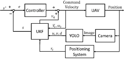
Figure 3: Block diagram of the controller.

V Simulations

V-A Environment Setup

In the simulation, a car is considered as a moving target and is tracked by a quadrotor, where the developed controller as well as the UKF are implemented. A camera is implemented on the quadrotor to provide visual feedback. Specifically, bounding boxes are generated in the image to enclose detected cars as shown in Fig. 2, which is achieved by a pretrained YOLO deep neural network. The simulation is conducted in the ROS framework (16.04, kinetic) with Gazebo simulator. In the simulation environment, the value of $A=4.6\text{m}\times 1.5\text{m},$ and the resolution of the image is $640$x$480$ with 50 fps. The intrinsic parameters matrix of the camera is

$$K = \left[\begin{array}[]{ccc}381.36&0&320.5\\ 0&381.36&240.5\\ 0&0&1\end{array}\right].$$

which is obtained by calibration.

A time moving window of width $N$ is set to be 150 with sampling rate of $50\>\text{sample}/\text{sec}$. The initial process and measurement noise covariance matrices are selected as $diag\left\{\left[20,\,20,\,500,\,0.0001,\,0.0001,\,0.0001\right]\right\}$ and $diag\left\{\left[0.08,\,0.08,\,0.02,\,5,\,5,\,5,\,1,\,1,\,1\right]\times 10^{-2}\right\},$ respectively, and the process noise covariance matrix is estimated online using (21).

The initial location of the car and the drone are $\left[\begin{array}[]{ccc}0&0&0\end{array}\right]^{T}$ and $\left[\begin{array}[]{ccc}0&5.5&1.0\end{array}\right]^{T}$ along with the initial orientations $\left[\begin{array}[]{ccc}0&0&0\end{array}\right]^{T}$ and $\left[\begin{array}[]{ccc}0&0&-\frac{pi}{2}\end{array}\right]^{T}$ in radians, respectively, all expressed in the global frame. The car is free to move on the $XY$ plane, and its velocity is specified based on the real-time user command.

V-B Simulation Results

Fig. 4 depicts the position estimate errors of the moving vehicle with simulation period of 223 seconds. The position estimate errors are reduced from 14% to 7% as the target moves from time-varying velocity to constant velocity, despite some noises. Note that in practice the drone may not react fast enough to the rapid change of velocity, in which the optical axis cannot remain facing right to the target, leading to a slight deviation in the depth estimate (i.e., $x_{3}$). Note that the position estimate error in the $Z$-axis increases as the velocity in the $Y$-axis increases. This can be attributed to the fact that the increasing velocity of the vehicle in the $Y$-axis causes the quadrotor to tilt forward for tracking, which breaks the assumption 2 that the optical axis is facing toward the side of the vehicle and leads to a large estimate error.

Remark 4.

In Gazebo environment, the velocity of the car is set below 4 m/s due to a large drag. As the speed of the car increases, the quadrotor accelerates with a tilt angle, which increases the chance of object detection failure. However, the problem can be resolved by expanding the training dataset with images from different angles of view, which will be part of the future work.

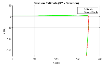
Figure 4: Estimate and ground truth of the target trajectory in the $XY$ plane in the global frame.

Fig. 5 depicts the velocity estimate errors of the moving vehicle. The estimate performance is slightly compromised when the vehicle is accelerated (i.e., due to the constant-velocity model utilized in the UKF), but better estimate performance can be expected by increasing the sensing rate for the UKF measurement. The increase of the velocity estimate error between 103-223 seconds can be attributed to the acceleration of the target in the $Y$-direction.

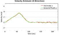
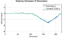
Figure 5: Estimate and ground truth of the target velocity in the $X$ and $Y$ direction of the global frame.

Fig. 6 depicts the estimate error without process noise estimation, where the constant covariance matrix $Q$ is same as the initial value. Compared to Fig. 5, using the estimated noise covariance matrix developed in (21) yields a better velocity estimate performance.

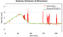
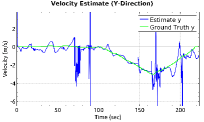
Figure 6: Estimate and ground truth of the target velocity without estimation of noise covariance matrix.

VI Conclusion

In this work, a motion controller for a camera on an UAV is developed to track a dynamic target with unknown motion and without motion constraint. The unknown target motion is estimated in the developed UKF with process noise covariance matrix estimated based on the past data within a moving window, and the intermittent measurement caused by YOLO detection is addressed. The estimated target velocity is then included as a feedforward term in the developed controller to improve tracking performance. Compared to the case without noise estimation, the developed approach is proven to obtain better tracking performance. Although Assumption 2 is rigorous in practice, this work is the first one to prove the feasibility of the overall control architecture, and future work will be relaxing the assumption by training a YOLO network to detect the target from any angles. Additionally, eliminating the knowledge of the ground truth will be another future works.

References

- [1] N. R. Gans, A. Dani, and W. E. Dixon, “Visual servoing to an arbitrary pose with respect to an object given a single known length,” in Proc. Am. Control Conf., Seattle, WA, USA, Jun. 2008, pp. 1261–1267.
- [2] A. Dani, N. Gans, and W. E. Dixon, “Position-based visual servo control of leader-follower formation using image-based relative pose and relative velocity estimation,” in Proc. Am. Control Conf., St. Louis, Missouri, Jun. 2009, pp. 5271–5276.
- [3] V. Chitrakaran, D. M. Dawson, W. E. Dixon, and J. Chen, “Identification of a moving object’s velocity with a fixed camera,” Automatica, vol. 41, pp. 553–562, 2005.
- [4] A. Stroupe, M. Martin, and T. Balch, “Distributed sensor fusion for object position estimation by multi-robot systems,” in Proc. IEEE Int. Conf. Robotics and Automation, Seoul, South Korea, May 2001, pp. 1092–1098.
- [5] A. Kamthe, L. Jiang, M. Dudys, and A. Cerpa, “Scopes: Smart cameras object position estimation system,” in EWSN ’09, Berlin, Heidelberg, Feb. 2009, pp. 279–295.
- [6] H. S. Ahn and K. H. Ko, “Simple pedestrian localization algorithms based on distributed wireless sensor networks,” IEEE Trans. Ind. Electron., vol. 56, no. 10, pp. 4296–4302, Mar. 2009.
- [7] J. Schlichenmaier, N. Selvaraj, M. Stolz, and C. Waldschmidt, “Template matching for radar-based orientation and position estimation in automotive scenarios,” in Proc. IEEE MTT-S Int. Conf. Microw. Intell. Mobility (ICMIM), Nagoya, Japan, Mar. 2017, pp. 95–98.
- [8] Z. Huang, W. Liu, and J. Zhong, “Estimating the real positions of objects in images by using evolutionary algorithm,” in Proc. Int. Conf. Mach. Vis. Inf. Technol., Singapore, Feb. 2017, pp. 34–39.
- [9] J. Thomas, J. Welde, G. Loianno, K. Daniilidis, and V. Kumar, “Autonomous flight for detection, localization, and tracking of moving targets with a small quadrotor,” IEEE Robot. Autom. Lett., vol. 2, no. 3, pp. 1762–1769, Jul. 2017.
- [10] E. Palazzolo and C. Stachniss, “Information-driven autonomous exploration for a vision-based mav,” in Proc. of the ISPRS Int. Conf. on Unmanned Aerial Vehicles in Geomatics (UAV-g), Bonn, Germany, Sep. 2017, pp. 59–66.
- [11] D. Scaramuzza, M. Achtelik, L. Doitsidis, F. Fraundorfer, E. Kosmatopoulos, A. Martinelli, M. Achtelik, M. Chli, S. Chatzichristofis, L. Kneip, D. Gurdan, L. Heng, G. Lee, S. Lynen, L. Meier, M. Pollefeys, A. Renzaglia, R. Siegwart, J. Stumpf, P. Tanskanen, C. Troiani, and S. Weiss, “Vision-controlled micro flying robots: From system design to autonomous navigation and mapping in gps-denied environments,” IEEE Robot. Autom. Mag., vol. 21, no. 3, pp. 26–40, Aug. 2014.
- [12] V. K. Chitrakaran and D. M. Dawson, “A lyapunov-based method for estimation of euclidean position of static features using a single camera,” in Proc. Am. Control Conf., New York, NY, USA, Jul. 2007, pp. 1988–1993.
- [13] D. Braganza, D. M. Dawson, and T. Hughes, “Euclidean position estimation of static features using a moving camera with known velocities,” in Proc. IEEE Conf. Decis. Control, New Orleans, LA, USA, Dec 2007, pp. 2695–2700.
- [14] A. P. Dani, N. R. Fischer, and W. E. Dixon, “Single camera structure and motion,” IEEE Transactions on Automatic Control, vol. 57, no. 1, pp. 238–243, Jan. 2012.
- [15] A. Dani, Z. Kan, N. Fischer, and W. E. Dixon, “Structure and motion estimation of a moving object using a moving camera,” in Proc. Am. Control Conf., Baltimore, MD, 2010, pp. 6962–6967.
- [16] A. Dani, Z. Kan, N. Fischer, and W. E. Dixon, “Structure estimation of a moving object using a moving camera: An unknown input observer approach,” in Proc. IEEE Conf. Decis. Control, Orlando, FL, 2011, pp. 5005–5012.
- [17] A. Parikh, T.-H. Cheng, and W. E. Dixon, “A switched systems approach to image-based localization of targets that temporarily leave the field of view,” in Proc. IEEE Conf. Decis. Control, 2014, pp. 2185–2190.
- [18] A. Parikh, T.-H. Cheng, and W. E. Dixon, “A switched systems approach to vision-based localization of a target with intermittent measurements,” in Proc. Am. Control Conf., Jul. 2015, pp. 4443–4448.
- [19] A. Parikh, T.-H. Cheng, H.-Y. Chen, and W. E. Dixon, “A switched systems framework for guaranteed convergence of image-based observers with intermittent measurements,” IEEE Trans. Robot., vol. 33, no. 2, pp. 266–280, April 2017.
- [20] K. Zhang, J. Chen, B. Jia, and Y. Gao, “Velocity and range identification of a moving object using a static-moving camera system,” in IEEE Conf. Decis. Control, Las Vegas, NV, USA, Dec. 2016, pp. 7135–7140.
- [21] J. Redmon and A. Farhadi, “Yolov3: An incremental improvement,” arXiv preprint arXiv:1804.02767, Tech. Rep., 2018.
- [22] S. Gao, G. Hu, and Y. Zhong, “Windowing and random weighting-based adaptive unscented kalman filter,” Int. J. Adapt. Control Signal Process., vol. 29, no. 2, pp. 201–223, Feb. 2015.
- [23] E. A. Wan and R. van der Menve, “The unscented kalman filter for nonlinear estimation,” in Proc. IEEE 2000 Adaptive Syst. Signal Process., Commun., Control Symp., Lake Louise, Alberta, Canada, Oct. 2000, pp. 153–158.
- [24] F. Chaumette and S. Hutchinson, “Visual servo control part I: Basic approaches,” IEEE Rob. Autom. Mag., vol. 13, no. 4, pp. 82–90, 2006.
- [25] N. Shahriari, S. Fantasian, F. Flacco, and G. Oriolo, “Robotic visual servoing of moving targets,” in Proc. IEEE/RSJ Int. Conf. Intell. Robots Syst., Tokyo, Japan, Nov. 2013, pp. 77–82.
- [26] J. Pestana, J. L. Sanchez-Lopez, S. Saripall, and P. Campoy, “Computer vision based general object following for gps-denied multirotor unmanned vehicles,” in Am. Control Conf., Portland, OR, USA, Jun. 2014, pp. 1886–1891.