An End-to-End Learning-based Cost Estimator

Abstract

Cost and cardinality estimation is vital to query optimizer, which can guide the plan selection. However traditional empirical cost and cardinality estimation techniques cannot provide high-quality estimation, because they cannot capture the correlation between multiple columns. Recently the database community shows that the learning-based cardinality estimation is better than the empirical methods. However, existing learning-based methods have several limitations. Firstly, they can only estimate the cardinality, but cannot estimate the cost. Secondly, convolutional neural network (CNN) with average pooling is hard to represent complicated structures, e.g., complex predicates, and the model is hard to be generalized.

To address these challenges, we propose an effective end-to-end learning-based cost estimation framework based on a tree-structured model, which can estimate both cost and cardinality simultaneously. To the best of our knowledge, this is the first end-to-end cost estimator based on deep learning. We propose effective feature extraction and encoding techniques, which consider both queries and physical operations in feature extraction. We embed these features into our tree-structured model. We propose an effective method to encode string values, which can improve the generalization ability for predicate matching. As it is prohibitively expensive to enumerate all string values, we design a patten-based method, which selects patterns to cover string values and utilizes the patterns to embed string values. We conducted experiments on real-world datasets and experimental results showed that our method outperformed baselines.

1 Introduction

Query optimizer is a vital component of database systems, which aims to select an optimized query plan for a SQL query. However, recent studies show that the classical query optimizer [15, 16, 20] often generates sub-optimal plans due to poor cost and cardinality estimation. First, traditional empirical cost/cardinality estimation techniques cannot capture the correlation between multiple columns, especially for a large number of tables and columns. Second, the cost model requires to be fine-tuned by DBAs.

Recently, the database community attempts to utilize machine learning models to improve cardinality estimation. MSCN [14] adopts the convolutional neural network to estimate the cardinality. However, this method has three limitations. Firstly, it can only estimate the cardinality, but cannot estimate the cost. Secondly, the deep neural network with average pooling is hard to represent complicated structures, e.g., complex predicates and tree-structured query plan, and thus the model is hard to be generalized to support most of SQL queries. Thirdly, although MSCN outperforms PostgreSQL in cardinality estimation, its performance can be further improved. For example, on the JOB-LIGHT workload, the mean error is over 50 and the max error is over 1,000. We can improve them to 24.9 and 289 respectively.

There are four challenges to design an effective learning-based cost estimator. First, it requires to design an end-to-end model to estimate both cost and cardinality. Second, the learning model should capture the tree-structured information of the query plan, e.g., estimating the cost of a plan based on its sub-plans. Third, it is rather hard to support predicates with string values, e.g., predicate "not LIKE ‘%(co-production)%’", if we don’t know which values contain pattern ‘(co-production)’. As the string values are too sparse, it is rather hard to embed the string values into the model. Fourth, the model should have a strong generalization ability to support various of SQL queries.

To address these challenges, we propose an end-to-end learning-based cost estimation framework by using deep neural network. We design a tree-structured model that can learn the representation of each sub-plan effectively and can replace traditional cost estimator seamlessly. The tree-structured model can also represent complex predicates with both numeric values and string values.

In summary, we make the following contributions.

(1) We develop an effective end-to-end learning-based cost estimation framework based on a tree-structured model, which can estimate both cost and cardinality simultaneously. To the best of our knowledge, this is the first end-to-end cost estimator based on deep learning (see Section 3).

(2) We propose effective feature extraction and encoding techniques, which consider both queries and physical execution in feature extraction. We embed these features into our tree-structured model, which can estimate the cost and cardinality utilizing the tree structure (see Section 4).

(3) For predicates with string values, we propose an effective method to encode string values for improving the generalization ability. As it is prohibitively expensive to enumerate all possible string values, we design a pattern-based method, which selects patterns to cover string values and utilizes the patterns to embed the string values (see Section 5).

(4) We conducted experiments on real-world datasets, and experimental results showed that our method outperformed existing approaches (see Section 6).

2 Related Work

Traditional Cardinality Estimation. Traditional cardinality estimation techniques can be broadly classified into three classes. The first is histogram-based methods [13]. The core idea is to divide the cell values into equal depth or equal width buckets, keep the cardinality of each bucket, and estimate the cardinality according to the buckets. The method is easy to implement and has been widely used in commercialized databases. However, it is not effective to estimate the correlations between different columns. The second is sketching, which aims to solve distinct cardinality estimation problem, including FM [7], MinCount [10], LinearCount [27], LogLog [6], HyperLogLog [8]. The basic idea first maps the tuple values to bitmaps, then counts the continuous zeros or the number of hitting for each position, and finally infers the approximate number of distinct values. These methods can estimate the distinct number of rows for each dataset effectively. However, they are not suitable for estimating range query. The third is sampling-based methods [18, 25, 29, 16]. These methods utilize the data samples to estimate the cardinality. In order to address the sample vanishing problem (valid samples decrease rapidly for joins), [16] proposed index-based sampling. Sampling methods improve the accuracy of cardinality estimation, but they bring space overhead and only be adopted by in-memory database like HyPer [24]. Another limitation of this method is 0-tuple problem, i.e., when a query is sparse, if the bitmap equals to 0, the sample is invalid.

Traditional Cost Model. Traditional cost estimation is estimated by combining multiple factors like cost of sequential page fetch, cost of random page fetch, cost of CPU cost of processing a tuple and cost of performing operation. Firstly, these factors are highly correlated to the cardinality of data affected by the query. Secondly, the weight of each factor has to be tuned. There are some works focusing the cost model tuning [28, 19, 15], and [15] conducted experiments on the IMDB dataset to show that cardinality estimation is much more crucial than the cost model for cost estimation and query optimization.

Learning-based Cardinality Estimation. The database community starts to solve this problem by using learning-based method like statistic machine learning or deep neural network. The first learning based work on cardinality estimation [21] first classifies queries according to the query structure (join condition, attributes in predicates etc.), and then trains a model on the values of the predicates, but the model is ineffective to train on unknown structured query. The state-of-the-art method [14] trains a multi-set convolutional network on queries, but this method is not suitable for query optimization, because the query-based encoding is too tricky when optimizing on a tree structure, and the generalization is limited. [26] proposed a vision of training representation for the join tree with reinforcement learning. However, this method does not support query plans with a complex tree structure and cannot support complex queries.

Learning-based Performance Prediction. There are several works on performance prediction by using machine learning and statistics [4, 28, 17, 9, 30], but they all require experts to select the features according to operation properties. A deep learning based approach [22] is also proposed. However, this method must take the estimated cardinality and the cost of PostgreSQL as features without learning the semantic of predicates, and it is not an end-to-end solution.

3 Overview of End-to-end Cost Estimator

Cost estimation is to estimate the execution cost of a query plan, and the estimated cost is used by the query optimizer to select physical plans with low cost. Cardinality estimation is to estimate the number of tuples in the result of a (sub)query. In this section we propose the system overview of cost and cardinality estimation.

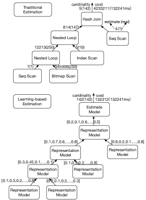
Figure 1: Comparison of Traditional Cost Estimation and Learning-based Cost Estimation.

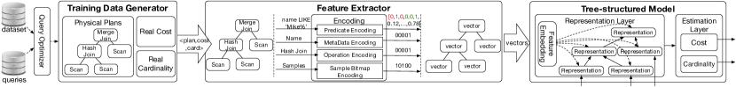
Figure 2: Architecture of learning-based cost estimator

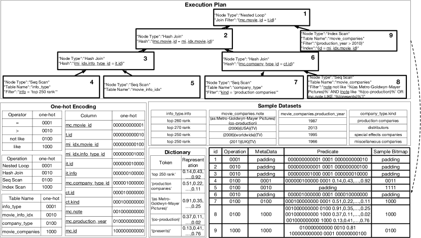
Figure 3: Running Example of query plan encoding

Traditional databases estimate the cost and cardinality using statistics. For filter operations, cardinality estimator (e.g., PostgreSQL[2], DB2[1]) estimates the cardinality using the histograms; for join operations, the cardinality is estimated by empirical functions with selectivity of joined tables (nodes) as variables. In Figure 1, the numbers on top of each node are estimated cardinality and real cardinality. We find that there exist large errors in traditional methods.

In general, we can effectively estimate the cardinality for leaf nodes (like Scan) by using the histogram; however, the error would be very large for joins because of the correlations between tables. Usually the more joins are, the larger error is. Unlike traditional cost estimation methods, our learning-based model can learn the correlation among multiple columns and tables, and the representation can retain accurate information on distribution of results even for the queries with dozens of operations.

Moreover, the query plan is a tree structure, and the plan is executed in a bottom-up manner. Intuitively, the cost/cardinality of a plan should be estimated based on its sub-plans. To this end, we design a tree-structured model that matches the plan naturally, where each model can be composed of some sub-models in the same way as a plan is made up of sub-plans. We use the tree-structured model to estimate the cost/cardinality of a plan in a bottom-up manner.

Learning-based Cost Estimator. The end-to-end learning-based tree-structured cost estimator includes three main components, including training data generator, feature extractor, and tree-structured model, as shown in Figure 2.

1) Training Data Generator generates training data based on the data and query workload. It first generates a large number of queries according to the potential join graph of the dataset and the predicates in the workload. Then for each query, it extracts a physical plan by the optimizer and gets the real cost/cardinality. Thus a training data is a triple $\langle$a physical plan, the real cost of the plan, the real cardinality of the plan$\rangle$.

2) Feature Extractor extracts useful features from the query plan, e.g., query operation and predicates. Each node in the query plan is encoded into feature vectors and each vector is organized into tensors. Then the tree-structured vectors are taken as input of the training model. For simple features, we can encode them by using one-hot vector or bitmap. While for complicated features, e.g., LIKE predicate, we encode each tuple $\langle$column, operator, operand$\rangle$ into vectors, by using a one-to-one mapping (see Section 4.1).

3) Tree-structured Model defines a tree-structured model which can learn representations for the (sub)plans, and the representations can be used in cost and cardinality estimation. The model is trained based on the training data, stores the updated parameters in the model, and estimates cost and cardinality for new query plans.

Workflow. For offline training, the training data are generated by Training Data Generator, which are encoded into tensors by Feature Extractor. Then the training data is fed into the Training Model and the model updates weights by back-propagating based on current training loss. The details of model training is discussed in Section 4.3.

For online cost estimation, when the query optimizer asks the cost of a plan, Feature Extractor encodes it in a up-down manner recursively. If the sub-plan rooted at the current node has been evaluated before, it extracts representation from Representation Memory Pool, which stores a mapping from a query plan to its estimated cost. If the current sub-plan is new, Feature Extractor encodes the root and goes to its children nodes. We input the encoded plan vector into Tree-structured Model, and then the model evaluates the cost and cardinality of the plan and returns them to the query optimizer. Finally, the estimator puts all the representations of ‘new’ sub-plans into Representation Memory Pool.

Figure 3 shows a running example of feature encoding for a plan extracted from the JOB workload. The plan is encoded as a vector using the one-hot encoding scheme, which considers both query and database samples. Then the vectors are taken as an input of the training model.

4 Tree-based Learning Model

In this section, we introduce a tree-structured deep neural network based solution for end-to-end cost estimation. We first introduce feature extraction in Section 4.1, and then discuss model design in Section 4.2. Finally we present the model training in Section 4.3.

4.1 Feature extraction and encoding

We first encode a query node as a node vector, and then transform the node vectors into a tree-structured vector.

There are four main factors that may affect the query cost, including the physical query operation, query predicate, meta data, and data. Next we discuss how to extract these features and encode them into vectors.

Operation is the physical operation used in the query node, including Join operation (e.g., Hash Join, Merge Join, Nested Loop Join); Scan operation (e.g., Sequential Scan, Bitmap Heap Scan, Index Scan, Bitmap Index Scan, Index Only Scan); Sort operation (e.g., Hash Sort, Merge Sort); Aggregation operation (e.g., Plain Aggregation, Hash Aggregation). These operations significantly affect the cost. Each operation can be encode as a one-hot vector. Figure 3 shows the one-hot vectors of different operations.

Predicate is the set of filter/join conditions used in a node. The predicate may contain join conditions like ‘movie.movie_id = mi_idx.movie_id’ or filter conditions like ‘production_year > 1988’. Besides the atomic predicates with only one condition, there may exist compound predicates with multiple conditions, like ‘production_year > 1988 AND production_year < 1993’. The predicates affect the query cost, because the qualified tuples will change after applying the predicates.

Table 1: Main Plan Operations

Operation	Features
$Aggregate$	$[Operator,Name_{keys}]$
$Sort$	$[Operator,Name_{keys}]$
$Join$	$[Operator,Predicate_{join}]$
$Scan$	$[Operator,Name_{table},Name_{index},$ $Predicate_{filter},SampleBitmap]$

Table 2: Features of Condition Operators

Operators	Features
and/or/not	$[Operator]$
=/!=/>/</LIKE/IN	$[Operator,Column,$ $Operand]$

Each atomic predicate is composed of three parts, Column, Operator, and Operand. Operator and Column can be encoded as one-hot vectors. For Operand, if it is a numeric value, we encode it by a normalized float; if it is string value, we encode it with a string representation (see Section 5 for details). Then the vector of an atomic predicate is the concatenation of the vectors for column, operator and operand. Table 2 shows the vector of each predicate.

For a compound predicate, we first generate a vector for each atomic predicate and then transfer multiple vectors into a vector using a one-to-one mapping strategy. There are multiple ways to transfer a tree structure to a sequence in a one-to-one mapping, and here we take the depth first search (DFS) as an example. We first transfer the nodes to a sequence using DFS, and then concatenate the vectors following the sequence order. Figure 4 shows an example of encoding a compound predicate. We transfer the nodes into a sequence in the visited order, where the solid lines with arrow represent forward search, and each dotted line represents one step backtracking. We append an empty node to the end of sequence for each dotted line. Thus, we can encode each distinct complex predicate tree as a unique vector and the compound predicate can be encoded as a tensor.

MetaData is the set of columns, tables and indexes used in a query node. We use a one-hot vector for columns, tables, and indexes respectively. Then the meta node vector is a concatenation of column vectors, table vectors and table vectors. (Note that a node may contain multiple tables, columns and indexes, and we can compute the unions of different vectors using the OR semantic.) We encode both meta data and predicate, because some nodes may not contain predicates. Figure 4 shows an example.

Sample Bitmap is a fix-sized 0-1 vector where each bit denotes whether the corresponding tuple satisfies the predicate of the query node. If the data tuple matches the predicate, the corresponding bit is 1; 0 otherwise. This feature is only included in nodes with predicates. Since it is expensive to maintain a vector for all tuples, we select some samples for each table and maintain a vector for the samples. Figure 4 shows an example of encoding sample data.

After encoding each node in the plan, we need to encode the tree-structured plan into a vector using a one-to-one mapping strategy. We also adopt the DFS method in the same ways as encoding compound predicates.

4.2 Model Design

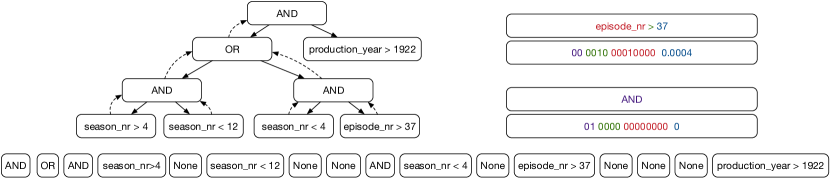
Figure 4: Predicates Encoding

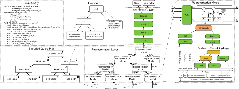
Figure 5: Two Level Tree Model

Our model is composed of three layers, embedding layer, representation layer and estimation layer as shown in Figure 5. Firstly, feature vectors in each plan node are large and sparse, we should condense them and extract high-dimensional information of features, and thus the embedding layer embeds the vector for each plan node. Secondly, the representation layer employs a tree-structured model, where each node is a representation model and the tree structure is the same as the plan. Each representation model learns two vectors (global vector and local vector) for the corresponding sub-plan, where the global vector captures the information of the sub-plan rooted at the node and the local vector captures the information of the node. Node that each representation model learns the two vectors based on the vectors of its two children and the feature vector of the corresponding node. Finally, based on the vectors of the root node, estimation layer estimates the cost and cardinality.

4.2.1 Embedding Layer

The embedding layer aims to embed a sparse vector to a dense vector.

As discussed in Section 4.1, there are 4 types of features, Operation, Metadata, Predicate and Sample Bitmap. Operation is a one-hot encoding vector, and Metadata and Sample Bitmap are bitmap vectors. We use a one-layer fully connected neural network with ReLU activator to embed these three vectors. However, the structure of the Predicate vector is complicated because it contains multiple AND/OR semantics, and we design an effective model to learn the representation of predicates.

Our goal is to estimate the number of tuples that satisfy a predicate. For an atomic predicate, we can directly use the vector. But for a compound predicate with multiple conditions, we need to learn the semantic of the predicates and the distribution of the results after applying the predicates on the dataset.

Consider a compound predicate with two atomic predicates using the AND semantic. We can estimate the number of results satisfying the predicate by the minimum number of estimated results satisfying the atomic predicates. Thus we use the min pooling layer to combine the two atomic predicates. Consider a compound predicate with two atomic predicates using the OR semantic. We can estimate the number of results satisfying the predicate by the maximum number of estimated results satisfying the atomic predicates. Thus we use the max pooling layer to combine the two atomic predicates.

In this way, we use a tree pooling to encode a predicate, where the tree structure is the same as the predicate tree structure. Particularly, the leaf node is a fully connected neural network, the OR semantic is replaced with the max pooling layer and the AND semantic is replaced with the min pooling layer. The advantages of this model are two folds. The first is that only the leaf nodes need to be trained so that it’s easy to do efficient batch training. The second is that this model converges faster and performs better.

Figure 4 shows a compound predicate and its embedded model. For leaf nodes, we use a fully connected neural network. For conjunction nodes, we use max pooling layer for ‘OR’ and min pooling layer for ‘AND’ which meet the semantic of ‘AND’ and ‘OR’.

Embedding Formulation. We denote features Operation, Metadata, Predicate and Sample Bitmap of $node_{t}$ as $O_{t},M_{t},P_{t},B_{t}$ respectively, and we denote each node of feature Predicate as $P_{t}$ with $P^{l}_{t}$ as its left child and $P^{r}_{t}$ right child. Embedding Model can be formalized as below. $E$ is the embedding output. $W$ is the weight of a fully connected neural network. $b$ is a bias.

$$\begin{split}&E=[embed(O_{t}),embed(M_{t}),embed(B_{t}),embed(P_{t})]\\ &embed(O_{t})=ReLU(W_{o}\cdot O_{t}+b_{o})\\ &embed(M_{t})=ReLU(W_{m}\cdot M_{t}+b_{m})\\ &embed(B_{t})=ReLU(W_{b}\cdot B_{t}+b_{b})\\ &embed(P_{t})=\left\{\begin{array}[]{lr}min(embed(P^{l}_{t}),embed(P^{r}_{t}))&type(P_{t})=AND,\\ max(embed(P^{l}_{t}),embed(P^{r}_{t}))&type(P_{t})=OR,\\ W_{p}\cdot P_{t}+b_{p}&type(P_{t})=Exp.\end{array}\right.\\ \end{split}$$

where $type(P_{t})$ is the type of a node, which includes AND, OR, and a predicate expression.

4.2.2 Representation Layer

Cost estimation has two main challenges – information vanishing and space explosion. First, it is easy to estimate the cost for simple operations, e.g., estimating the cost of a filtering predicate on a single table, but it is rather hard to estimate the cost of joining multiple tables, because the join space is large and the joined tuples are sparse. In other words, in leaf nodes, we can capture much information for single table processing. But for upper nodes in the query plan, the correlation among nodes may be lost and this is the information vanishing problem. Second, to retain enough information to capture the correlations among tables, it requires to store much more space and intermediate results. But the space grows exponentially and becomes prohibitively expensive for a large number of tables. This is the space explosion problem.

Representation layer aims to address these two problems, by capturing the global cost information from leaf nodes to the root and avoiding information loss (e.g., correlation between columns). The representation layer trains representation for sub-plan recursively, instead of using data sketch to represent intermediate results of sub-plans. The representation layer uses the representation vector learned from features to represent results of sub-plans. As Figure 5 shows, all the units in this layer are neural networks in the same structure and share common parameters and we call these units as representation models. Each representation model has three inputs, the embedding vector $E$, the representation vector $[G^{l}_{t-1},R^{l}_{t-1}]$ of its left child, and the representation vector $[G^{r}_{t-1},R^{r}_{t-1}]$ of its right child. (Note that for leaf nodes, we use zero vectors as their children vectors.) The output is $[G_{t},R_{t}]$.

The most important design issue in this layer is the choice of recurrent neural network. As a joint network of the tree-structured model, it decides which information to be passed over. A naive implementation is using fully connected neural network which takes as input the concatenate of local transformed features and its children’s output. However, the lost information would never be utilized by upper nodes any more. Therefore, representation model with naive neural networks suffers from gradient vanishing and gradient explosion problems.

Compared to naive deep neural network, LSTM cell can efficiently address these problems by using an extra information channel. The structure of LSTM cell is shown in Figure 5, where $G_{t}$ is the channel for long memory, $f_{t}$ controls which information should be forgot in the long memory. $k^{1}_{t}$ controls which information should be added into the long memory channel. $k^{2}_{t}$ controls which information in the memory channel should be taken as the representation of the sub-plans. As $G_{t}$ can be a path without any multiplication, LSTM avoids gradient vanishing. The forget gate of Sigmoid can help LSTM to address gradient explosion problem. The representation layer can be formalized as below:

$$\begin{split}&x_{t}=E\\ &G_{t-1}=(G^{l}_{t-1}+G^{r}_{t-1})/2\\ &R_{t-1}=(R^{r}_{t-1}+R^{r}_{t-1})/2\\ &f_{t}=Sigmoid(W_{f}\cdot[R_{t-1},x_{t}]+b_{f})\\ &k^{1}_{t}=Sigmoid(W_{k_{1}}\cdot[R_{t-1},x_{t}]+b_{k_{1}})\\ &r_{t}=tanh(W_{r}\cdot[R_{t-1},x_{t}]+b_{r})\\ &k^{2}_{t}=Sigmoid(W_{k_{2}}\cdot[R_{t-1},x_{t}]+b_{k_{2}})\\ &G_{t}=f_{t}\times G_{t-1}+k^{1}_{t}\times r_{t}\\ &R_{t}=k^{2}_{t}\times tanh(G_{t})\\ \end{split}$$

where $E$ is the vector, $W$ is a weight and $b$ is a bias.

4.2.3 Estimation Layer

The Estimation Layer is a two-layer fully connected neural network, and the activator is a ReLU function and the output layer is a sigmoid function to predict the normalized cardinality and cost. The output layer should be able to evaluate cost or cardinality for any sub-plan by its representation vector. This layer takes the representation $R_{t}$ of the upper model in Representation Layer as input, and can be formalized as below:

$$\begin{split}&cost^{\prime}=ReLU(W_{cost^{\prime}}\cdot R_{t}+b_{cost^{\prime}})\\ &card^{\prime}=ReLU(W_{card^{\prime}}\cdot R_{t}+b_{card^{\prime}})\\ &cost=Sigmoid(W_{cost}\cdot cost^{\prime}+b_{cost})\\ &card=Sigmoid(W_{card}\cdot card^{\prime}+b_{card})\\ \end{split}$$

As we need to estimate both cost and cardinality, we use multitask learning [5] in order to improve the generalization by using the domain information contained in the training signals of related tasks as an inductive bias. Parameter sharing is one of the most common implementation strategies for multitask learning, which means that we train several tasks simultaneously, and the models of these tasks share some network layers.

Since the cost of the query plan is correlated to the cardinality of each node in the plan tightly, we train the cost estimation task and cardinality estimation task simultaneously. These two tasks share common embedding layer and representation layer and we expect these two layers to learn general representations for both tasks, and the estimation layer can extract cost and cardinality from representations respectively. In this way, the generality of the learning model is better than training on cost only task, and thus the model can achieve much better performance.

4.3 Training Model

Training Data Generation. Our model has strong generalization ability. Given a dataset and a workload, e.g., IMDB, we generate potential join relations from the PK-FK index and query workload. According to the join graph, we select the number of tables ($N$) involved in the query workload, and then we select $N$ connected tables. For predicates, we generate numeric expressions and string expressions individually. For numeric expressions, we randomly select $M$ columns with numeric type in the chosen tables and select a value from dataset for each column. Then we pick operators from ‘$>,<,=,!=$’ for each column. While for expressions with string value, we first pick operators from ‘$=,!=,LIKE,NOT~{}LIKE,IN$’, and then select values from substring dictionary (see Section 5). After generating expressions for each table, we aggregate these expressions into complex predicates by using the ‘AND’/‘OR’ semantics. For projection, we select several columns in tables as outputs, and select MIN, MAX, COUNT or Non for each attribute. After we obtain all the training SQL queries, we get physical plans from DBMS by using plan analysis tools. Then we transform plans to sequences and divide them into mini-batches to train.

Loss Function. Our model trains cost and cardinality simultaneously. The loss function can be a linear combination of cost loss and cardinality loss, and the weight can be regarded as hyper-parameters. We try different loss weights in $\{0.1,0.2,0.5,1,2,5,10\}$, and pick the one with the lowest validation error by cross validation. In order to achieve high quality and accelerate convergence speed, we take the normalized true cardinality/cost as the targets. The loss functions are formalized as below:

$$\begin{split}loss=\frac{1}{n}\sum_{i}\bigl{(}\omega\cdot qerror(cost_{i},estimated\_cost_{i})+\\ qerror(card_{i},estimated\_card_{i})\bigr{)}\end{split}$$

where $n$ is the number of training queries, $cost_{i}$ and $card_{i}$ are respectively the real cost and cardinality, and $estimated\_cost_{i}$ and $estimated\_card_{i}$ are respectively the estimated cost and cardinality.

$$qerror(cost_{i},estimated\_cost_{i})=\frac{\max(cost_{i},estimated\_cost_{i})}{\min(cost_{i},estimated\_cost_{i})}$$

$$qerror(card_{i},estimated\_card_{i})=\frac{\max(card_{i},estimated\_card_{i})}{\min(card_{i},estimated\_card_{i})}$$

Batch Training. In a batch of training samples with size $\mathcal{N}$, let $\mathcal{D}$ denote the maximum depth of the tree structure. We change the depth-first encoding into width-first encoding, where the input of each batch is organized hierarchically which means the first dimension of the nodes tensor equals to $\mathcal{D}$ while not $\mathcal{N}$. An extra tensor is needed to represent the edge of different layers of trees where each element indicates positions of the left child and right child. For each time, the model batches nodes in certain level of encoded plan trees and trains them all at once. In this way, the model only needs to run LSTM cell for each level of trees ($\mathcal{D}$ times) instead of running for each node, which reduces the training and evaluating time by $\mathcal{O}(\frac{2^{\mathcal{D}}\mathcal{N}}{\mathcal{D}})$ times.

5 String Embedding

The distribution of numeric values can be learned, even though some values do not appear in the training data, because most numeric values are in a continuous space. For example, predicate $production\_year\in[1990,2000)$ can be inferred from $production\_year\in[1990,1995)$ and $production\_year\in[1995,2000)$. However, string values are sparse and discrete, and thus hard to learn. So it is much harder to learn the predicates with string values than predicates with numeric values.

There are four intuitive ways to represent a predicate with string values, including one-hot, selectivity, sample bitmap, hash bitmap. The one-hot embedding maps a string to a bit in the vector. However it cannot estimate an approximate result for unseen string values. The selectivity embedding first translates the selectivity of a string value into a numerical value, and then utilizes to the numeric value to embed the string. However, it can not reflect the details on which tuples satisfy the predicate. The sample bitmap embedding uses samples to embed a string value, i.e., the string value is 1 if the sample contains it; 0 otherwise. However, it suffers from the 0-tuple problem for sparse predicates. The hash bitmap embedding first initializes a zero vector $\mathcal{V}$, and then for each character in the string, calculates its hash value $\mathcal{H}$ and set position $\mathcal{H}\%|\mathcal{V}|$ in the bitmap as 1. The number of character types is small (e.g., only 60 distinct characters in the JOB workload, including numbers, characters, punctuations, and other special characters). Therefore, the embedding vectors with hundreds of bits could effectively avoid hash collision even for unseen strings. The hash-bitmap embedding carries the characters contained in a string, so we can know the approximate overlap of two strings by taking ‘AND’ on their hash bitmap. However, the hash bitmap embedding can only capture the similarity between two strings but cannot reveal the co-occurrences of two strings.

Embedding-based Method. In order to represent the distribution of the string values in a dataset, we need to learn representations for string values in the predicates, and the representations can capture the co-occurrences of strings that co-exist in the same tuple. There are two kinds of possible string predicates in a query. The first is exact matching predicate (e.g., using keywords ‘=’ and ‘IN’), and query strings in exact matching predicates will match the tuple values. The second is pattern matching predicate (e.g., using keywords ‘LIKE’), and query strings in pattern matching predicates match substrings of some values in the dataset. In this section, our goal is to pre-train all the substrings in the predicates so that each substring can be encoded by coexistence-aware representation. There are two challenges. The first is how to build a dictionary covering all the strings/substrings in both current and future workloads and the size of the dictionary is bounded. The second is how to maintain all the substrings in the dictionary to efficiently get the encoding of each string/substring with little space overhead. We first give the overview of the embedding method in Section 5.1, and then address these two challenges in Sections 5.2 and 5.3 respectively.

5.1 String Embedding Overview

Given a dataset and a query workload, we aim to encode all the strings/substrings that either are used in the current workload or will be used in the future workload. Thus we do not just encode the plain strings appearing in the query workload. Instead, we generalize the strings/substrings and generate some important rules which could extract all the strings/substrings in the query workload from the dataset. Then we extract all substrings that satisfy the rules and train a model to learn a representation for each string/substring. We take a collection of (sub)strings with the key values in one tuple as a sentence and use the skip-gram model [23] (a kind of model for word2vec) to train the string embedding. To efficiently get the embedding of each string in order to encode the queries online, we build an index with small space overhead and support fast prefix/suffix searching. Thus we address two challenges in string embedding.

Rule Generation. We find rules to generalize the (sub)strings in the query workload.

String Indexing. We use the patterns to extract all the substrings. Then we encode these substrings. To efficiently get the code of each substring, we construct trie indexes for storing all these substrings with their codes.

Table 3: Example of substring extraction

Predicate	Extraction
title LIKE ‘Din%’	"Dinos in Kas" $\rightarrow$ "Din"
title LIKE ‘Sch%’	"Schla in Tra" $\rightarrow$ "Sch"
title LIKE ‘%06%’	"(2002-06-29)" $\rightarrow$ "06"
title LIKE ‘%08%’	"(2014-08-26)" $\rightarrow$ "08"

Table 4: Candidate rules for "Dinos in Kas" $\rightarrow$ "Din%"

	Rules
"Din" $\rightarrow$ "Din"	$\langle Prefix,P_{t}(``Din"),3\rangle$ $\langle Prefix,P_{C}P_{t}(``in"),3\rangle$
"Dinos" $\rightarrow$ "Din"	$\langle Prefix,P_{t}(``D")P_{l},3\rangle$ $\langle Prefix,P_{C}P_{l},3\rangle$ $\langle Prefix,P_{C}P_{t}(``i")P_{l},3\rangle$ $\langle Prefix,P_{C}P_{t}(``in")P_{l},3\rangle$ $\langle Prefix,P_{t}(``Din")P_{l},3\rangle$
"Dinos " $\rightarrow$ "Din"	$\langle Prefix,P_{t}(``D")P_{l}P_{s},3\rangle$ $\langle Prefix,P_{C}P_{l}P_{s},3\rangle$ $\langle Prefix,P_{C}P_{t}(``i")P_{l}P_{s},3\rangle$ $\langle Prefix,P_{C}P_{t}(``in")P_{l}P_{s},3\rangle$ $\langle Prefix,P_{t}(``Din")P_{l}P_{s},3\rangle$
"Dinos in" $\rightarrow$ "Din"	$\langle Prefix,P_{t}(``D")P_{l}P_{s}P_{l},3\rangle$ $\langle Prefix,P_{C}P_{l}P_{s}P_{l},3\rangle$ $\langle Prefix,P_{C}P_{t}(``i")P_{l}P_{s}P_{l},3\rangle$ $\langle Prefix,P_{C}P_{t}(``in")P_{l}P_{s}P_{l},3\rangle$ $\langle Prefix,P_{t}(``Din")P_{l}P_{s}P_{l},3\rangle$
"Dinos in " $\rightarrow$ "Din"	$\langle Prefix,P_{t}(``D")P_{l}P_{s}P_{l}P_{s},3\rangle$ $\langle Prefix,P_{C}P_{l}P_{s}P_{l}P_{s},3\rangle$ $\langle Prefix,P_{C}P_{t}(``i")P_{l}P_{s}P_{l}P_{s},3\rangle$ $\langle Prefix,P_{C}P_{t}(``in")P_{l}P_{s}P_{l}P_{s},3\rangle$ $\langle Prefix,P_{t}(``Din")P_{l}P_{s}P_{l}P_{s},3\rangle$
"Dinos in Kas" $\rightarrow$ "Din"	$\langle Prefix,P_{t}(``D")P_{l}P_{s}P_{l}P_{s}P_{C}P_{l},3\rangle$ $\langle Prefix,P_{C}P_{l}P_{s}P_{l}P_{s}P_{C}P_{l},3\rangle$ $\langle Prefix,P_{C}P_{t}(``i")P_{l}P_{s}P_{l}P_{s}P_{C}P_{l},3\rangle$ $\langle Prefix,P_{C}P_{t}(``in")P_{l}P_{s}P_{l}P_{s}P_{C}P_{l},3\rangle$ $\langle Prefix,P_{t}(``Din")P_{l}P_{s}P_{l}P_{s}P_{C}P_{l},3\rangle$

Table 5: Candidate rules for "(2002-06-29)" $\rightarrow$ "%06%"

	Rules
"06" $\rightarrow$ "06"	$\langle Prefix,P_{t}(``06"),2\rangle$ $\langle Prefix,P_{n}P_{t}(``6"),2\rangle$ $\langle Prefix,P_{n},2\rangle$ $\langle Prefix,P_{t}(``0")P_{n},2\rangle$
"06-" $\rightarrow$ "06"	$\langle Prefix,P_{t}(``06")P_{t}(``\mathcal{-}"),2\rangle$ $\langle Prefix,P_{n}P_{t}(``6")P_{t}(``\mathcal{-}"),2\rangle$ $\langle Prefix,P_{n}P_{t}(``\mathcal{-}"),2\rangle$ $\langle Prefix,P_{t}(``0")P_{n}P_{t}(``\mathcal{-}"),2\rangle$
"06-29" $\rightarrow$ "06"	$\langle Prefix,P_{t}(``06")P_{t}(``\mathcal{-}")P_{n},2\rangle$ $\langle Prefix,P_{n}P_{t}(``6")P_{t}(``\mathcal{-}")P_{n},2\rangle$ $\langle Prefix,P_{n}P_{t}(``\mathcal{-}")P_{n},2\rangle$ $\langle Prefix,P_{t}(``0")P_{n}P_{t}(``\mathcal{-}")P_{n},2\rangle$
"06-29)" $\rightarrow$ "06"	$\langle Prefix,P_{t}(``06")P_{t}(``\mathcal{-}")P_{n}P_{t}(``)"),2\rangle$ $\langle Prefix,P_{n}P_{t}(``6")P_{t}(``\mathcal{-}")P_{n}P_{t}(``)"),2\rangle$ $\langle Prefix,P_{n}P_{t}(``\mathcal{-}")P_{n}P_{t}(``)"),2\rangle$ $\langle Prefix,P_{t}(``0")P_{n}P_{t}(``\mathcal{-}")P_{n}P_{t}(``)"),2\rangle$
"06" $\rightarrow$ "06"	$\langle Suffix,P_{t}(``06"),2\rangle$ $\langle Suffix,P_{n}P_{t}(``6"),2\rangle$ $\langle Suffix,P_{n},2\rangle$ $\langle Suffix,P_{t}(``0")P_{n},2\rangle$
"-06" $\rightarrow$ "06"	$\langle Suffix,P_{t}(``\mathcal{-}")P_{t}(``06"),2\rangle$ $\langle Suffix,P_{t}(``\mathcal{-}")P_{n}P_{t}(``6"),2\rangle$ $\langle Suffix,P_{t}(``\mathcal{-}")P_{n},2\rangle$ $\langle Suffix,P_{t}(``\mathcal{-}")P_{t}(``0")P_{n},2\rangle$
"2002-06" $\rightarrow$ "06"	$\langle Suffix,P_{n}P_{t}(``\mathcal{-}")P_{t}(``06"),2\rangle$ $\langle Suffix,P_{n}P_{t}(``\mathcal{-}")P_{n}P_{t}(``6"),2\rangle$ $\langle Suffix,P_{n}P_{t}(``\mathcal{-}")P_{n},2\rangle$ $\langle Suffix,P_{n}P_{t}(``\mathcal{-}")P_{t}(``0")P_{n},2\rangle$
"(2002-06" $\rightarrow$ "06"	$\langle Suffix,P_{t}(``(")P_{n}P_{t}(``\mathcal{-}")P_{t}(``06"),2\rangle$ $\langle Suffix,P_{t}(``(")P_{n}P_{t}(``\mathcal{-}")P_{n}P_{t}(``6"),2\rangle$ $\langle Suffix,P_{t}(``(")P_{n}P_{t}(``\mathcal{-}")P_{n},2\rangle$ $\langle Suffix,P_{t}(``(")P_{n}P_{t}(``\mathcal{-}")P_{t}(``0")P_{n},2\rangle$

5.2 Rule Generation

Rule Definition. Each rule can be expressed as a program. We borrow the idea from domain specific language (DSL) proposed by Gulwani [11, 12] to define a rule, which is composed of three parts, pattern, string function and size. The pattern matches substrings of tuples in the dataset. The string function decides which substring of tuples should be extracted. The size indicates the length of the substring to be extracted.

The pattern includes capital letters $\mathcal{P}_{C}$, lowercase letters $\mathcal{P}_{l}$, numerical values $\mathcal{P}_{n}$, white spaces $\mathcal{P}_{s}$ and exact matching token $\mathcal{P}_{t}(T)$ which can only match a specific substring $T$. The string function includes two types, Prefix and Suffix. Prefix extracts the prefix of the string and Suffix extracts the suffix of the string. The rule can be formalized as below:

$$\begin{split}&\mathcal{F}\in\{\text{Prefix, Suffix}\}\\ &\mathcal{P}\in combination\{\mathcal{P}_{C},\mathcal{P}_{l},\mathcal{P}_{s},\mathcal{P}_{n},\mathcal{P}_{t}(T)\}\\ &\qquad\mathcal{P}_{C}=[A\mathcal{-}Z]+\\ &\qquad\mathcal{P}_{l}=[a\mathcal{-}z]+\\ &\qquad\mathcal{P}_{s}=whitespace+\\ &\qquad\mathcal{P}_{n}=[0\mathcal{-}9]+\\ &\qquad\mathcal{P}_{t}(T)=T\\ &rule=\langle\mathcal{F},\mathcal{P},\mathcal{L}\rangle\end{split}$$

where $\mathcal{P}$ is a pattern, $\mathcal{F}$ is a string function, and $\mathcal{L}$ is the length of a substring.

Rule Candidate Set. Given a query string in the predicate and a tuple string in the dataset, we first find all substrings of the tuple string that match the query string. Then for each matched substring, we generate all possible patterns that map the query string to the substring, by enumerating all possible combinations of patterns in $\mathcal{P}_{C}$, $\mathcal{P}_{l}$, $\mathcal{P}_{n}$, $\mathcal{P}_{s}$, $\mathcal{P}_{t}(T)$. If the predicate is prefix search (e.g., LIKE “Din%”), then for each possible pattern $p$, we generate a rule (prefix, $p$, size of the query string). If the predicate is suffix search, we generate a rule (suffix, $p$, size of the query string). If the predicate is substring search, we generate a rule (prefix/suffix, $p$, size of the query string), based on how the query string matches the substring. All the possible rules will form a Rule Candidate Set.

For example, Table 4 shows some predicates and their sample substrings where ‘Dinos in Kas’ is a value selected by the predicate "title LIKE ‘Din%’". Table 5 shows the rules for “%06%”.

Rule Selection. Based on the candidate rules, we aim to find an optimal set of rules, which finds the minimum number of rules to cover the query workload. However, if we select those too general rules, the number of substrings would be too large. Therefore, we set an upper bound for the total number of extracted substrings.

Let $\mathcal{R}$ denote a subset of candidate rule set $C_{\mathcal{R}}$ which could cover the strings in the workload, $S_{\mathcal{R}}$ be the set of substrings which are extracted by rules in $\mathcal{R}$ from the datasets, and $S_{\mathcal{W}}$ is the set of strings in the workload. We aim to minimize the size of $\mathcal{R}$ with an upper bound $\mathcal{B}$ where $S_{\mathcal{R}}$ contains all strings in $S_{\mathcal{W}}$. The problem is formalized below:

$$\begin{split}&\mathcal{R}=arg\min_{\mathcal{R}\subseteq C_{\mathcal{R}}}(|\mathcal{R}|)\\ &\mathrm{s.t.}\quad|S_{\mathcal{R}}|<\mathcal{B},S_{\mathcal{W}}\subseteq S_{\mathcal{R}}\\ \end{split}$$

This is an NP-hard problem by a reduction from a classical set cover problem (SCP)[3]. Now the universe is $S_{\mathcal{W}}$, and the subset is $S_{r}\cap S_{\mathcal{W}}$ where $r\in C_{\mathcal{R}}$. We also have that the union of subsets $\sum_{r\in C_{\mathcal{R}}}S_{r}\cap S_{\mathcal{W}}$ equals to the universe $S_{\mathcal{W}}$. Our target is to find the minimum number of subsets to cover the universe.

We propose a greedy solution to address this problem approximately. We add a rule $r$ to the rule set $\mathcal{R}$ covering the most substrings in $S_{\mathcal{W}}$ each time. If the total size of $S_{\mathcal{R}}$ exceeds the bound $\mathcal{B}$, we remove the rule $r$ with the largest $S_{r}$ and repeat. The pseudo code of the algorithm is shown in Algorithm 1.

For example, consider three rules in the Table 5, $\langle Prefix,P_{t}(``06"),2\rangle$, $\langle Prefix,P_{n},2\rangle$ and $\langle Suffix,P_{t}(``(")P_{n}P_{t}(``\mathcal{-}")P_{n},2\rangle$. The first rule can only extract ‘06’. The second rule can extract 6 substrings including {‘2002’, ‘06’, ‘29’, ‘2014’, ‘08’, ‘26’}. The third rule can extract {‘06’, ‘08’}. The third rule would be selected in our algorithm, because it’s general and will not extract too many substrings.

Input: Candidate rules set $C_{\mathcal{R}}$; An upper bound $B$; All string sets $S_{r}$ extracted by rules in $C_{\mathcal{R}}$ from datasets; Set of strings in the workload $S_{\mathcal{W}}$;

Output: Selected rule set $\mathcal{R}$

Initialize rule set $\mathcal{R}=\emptyset$;AlgoLine0.1

for r $\in$ $C_{\mathcal{R}}$ do  $r$ $\rightarrow$ $\langle r,S_{r},|S_{r}\mathcal{-}S_{\mathcal{W}}|\rangle$; AlgoLine0.2

  Sort $C_{\mathcal{R}}$ in descending order of $|S_{r}\mathcal{-}S_{\mathcal{W}}|$;AlgoLine0.3

while $S_{\mathcal{W}}-S_{\mathcal{R}}\neq\emptyset$ or $C_{\mathcal{R}}\neq\emptyset$ do  $r^{*}$,$S_{r^{*}}$,$\mathcal{L}^{*}$ = $pop(C_{\mathcal{R}})$; AlgoLine0.4

$\mathcal{R}$ = add($\mathcal{R}$, $r^{*}$);AlgoLine0.5

$S_{\mathcal{R}}$ = add($S_{r^{*}}$,$S_{\mathcal{R}}$);AlgoLine0.6

if $|S_{\mathcal{R}}|\geq\mathcal{B}$ then  $r^{\prime}$ = $arg\min_{r\in\mathcal{R}}\frac{|S_{\mathcal{R}}\cap S_{\mathcal{W}}|}{|S_{\mathcal{R}}|}$; AlgoLine0.7

$\mathcal{R}$ = remove($r^{\prime}$,$\mathcal{R}$);AlgoLine0.8

$S_{\mathcal{R}}$ = remove($S_{r^{\prime}}$,$S_{\mathcal{R}}$);AlgoLine0.9

    return $\mathcal{R}$;AlgoLine0.10

Algorithm 1 RuleSelection

10

10

10

10

10

10

10

10

10

10

Based on the selected rules, we generate all the string values in the dataset and store the extracted substrings in the dictionary.

5.3 String Indexing

Figure 6: Trie Index Structure

There could be a large number of strings and it is expensive to maintain all strings in a dictionary. In order to avoid storing a huge number of duplicate tokens, we build a trie index to store the mapping from a string to its code.

String Indexing. We use both prefix trie and suffix trie as string index. Figure 6 shows an example of a prefix trie. Substrings extracted by the prefix function are stored into prefix trie and substrings extracted by the suffix function are stored in suffix trie. In this way, each string in the dictionary must have one or two paths in the index. Leaf nodes of the trie index are representation vectors of strings.

Online Searching. When a new query comes, there may be some query strings which do not exist in the dictionary. These query strings may be in prefix searching (LIKE s%), suffix searching(LIKE %s), keyword searching(=) or containment searching(LIKE %s%). For prefix search, we search the longest prefix of the query string. For suffix search, we search the longest suffix of the query string. For other searches, we search both the longest prefix and longest suffix of the query string, and then pick the longest one as the representation. Considering "title LIKE ‘Dino%’", we search the prefix trie and take the representation of ‘Din’ as the representation of ‘Dino’. In this way, we can encode queries online quickly.

6 Experiments

We conduct extensive experiments to evaluate our method from three aspects. (1) The effectiveness of our tree-structured model on cost and cardinality estimation. (2) The effectiveness of predicates embedding. (3) The efficiency of our model on cost estimation.

6.1 Experiment Setting

Datasets. We use the real dataset IMDB and the real workload JOB. It is much harder to estimate the cardinality and cost on the IMDB dataset than TPC-H, because of the correlations and skew distributions of the real-world data. The IMDB dataset includes 22 tables, which are joined on primary keys and foreign keys. We build indexes on primary keys. We use two types of query workloads.

(1) The first workload contains predicates with numeric attributes only [14]. It contains synthesis workload, scale workload and JOB-light workload. We adopt all three workloads with only numeric predicates. The Synthesis workload contains queries with 2 joins at most and there are 5000 queries. The Scale workload contains queries with 0-4 joins and there are 500 queries. The JOB-light workload contains queries with 1-4 joins, and there are 70 queries.

(2) The second workload contains complex predicates with string attributes. We generate training data based on the join graph of IMDB and predicates used in the JOB workloads. We take 90% of generated queries as training data and 10% as validation data. The 113 JOB queries are taken as the test workload. Different from previous cardinality estimation methods [14], we obtain query plans from PostgreSQL, and use the plans to train our model.

Metrics. The $mean$ is the average errors of all the tested queries. The $max$ is the maximum errors in the tested workload. The $median$ is the median of errors of all the tested queries. The $\mathcal{K}th$ is the average of top-{1-$\mathcal{K}\%$} largest errors in the tested workload.

Environment. We use a machine with Intel(R) Xeon(R) CPU E5-2630 v4, 128GB Memory, and GeForce GTX 1080.

Table 6: Methods on numeric workloads

Methods	Target	Represent	Predicate	Estimate	Sample
PGCard	Card	No	No	No	No
MSCNCard	Card	No	No	SING	Yes
MSCNNSCard	Card	No	No	SING	No
TLSTMNSCard	Card	LSTM	LSTM	SING	No
TNNCard	Card	NN	LSTM	SING	Yes
TLSTMCard	Card	LSTM	LSTM	SING	Yes
PGCost	Cost	No	No	No	No
MSCNCost	Cost	No	No	SING	Yes
TLSTMCost	Cost	LSTM	LSTM	SING	Yes
TNNMCost	Cost	NN	LSTM	MULT	Yes
TLSTMMCost	Cost	LSTM	LSTM	MULT	Yes

Table 7: Cardinality errors on numeric workloads

JOB-light	median	90th	95th	99th	max	mean
PGCard	7.93	164	1104	2912	3477	174
MSCNCard	3.82	78.4	362	927	1110	57.9
TNNCard	2.95	76.8	275	799	902	49.8
TLSTMCard	3.73	50.8	157	256	289	24.9
Synthetic	median	90th	95th	99th	max	mean
PGCard	1.69	9.57	23.9	465	373901	154
MSCNCard	1.18	3.32	6.84	30.51	1322	2.89
TNNCard	1.40	5.51	10.7	43.1	441	3.57
TLSTMCard	1.20	3.21	6.12	25.2	357	2.87
Scale	median	90th	95th	99th	max	mean
PGCard	2.59	200	540	1816	233863	568
MSCNCard	1.42	37.4	140	793	3666	35.1
TNNCard	1.59	58.7	141	573	2238	31.3
TLSTMCard	1.43	38.8	139	469	1892	28.1

Table 8: Cost errors on numeric workloads

JOB-light	median	90th	95th	99th	max	mean
PGCost	26.8	332	696	2740	3020	173
MSCNCost	4.75	11.3	40.1	563	987	27.4
TLSTMCost	3.66	32.1	80.3	445	583	17
TNNMCost	2.06	25.5	134	293	401	19.1
TLSTMMCost	1.85	13.2	22.9	95	123	5.81
Synthetic	median	90th	95th	99th	max	mean
PGCost	15.1	65.1	173	1200	8040	62.7
MSCNCost	3.14	7.43	18.1	65.8	739	10.3
TLSTMCost	1.56	4.47	10.7	57.7	689	4.45
TNNMCost	1.49	4.50	10.6	61.5	718	4.35
TLSTMMCost	1.49	4.33	10.2	55.8	624	4.16
Scale	median	90th	95th	99th	max	mean
PGCost	13.3	38.9	81.1	718	1473	35.7
MSCNCost	1.79	10.6	27.1	88.8	1027	8.22
TLSTMCost	1.58	5.51	14.4	70.1	611	5.21
TNNMCost	1.61	5.37	13.5	72.7	714	5.53
TLSTMMCost	1.56	5.56	12.2	68.6	254	4.41

6.2 Effectiveness on workloads with only numeric predicates

Methods. Table 8 shows the methods evaluated on workloads with numeric predicates. The Target is cardinality or cost. The Represent is the model we use as representation layer described in Section 4.2.2, including LSTM and Neural Network. The Predicate is the model we use as a predicate embedding layer described in Section 4.2.1, including Min-Max Pooling model and tree-LSTM. The Estimate is the model we use as an estimation layer described in Section 4.2.3, and it indicates whether using multitask training or using cost estimation only. The Sample indicates whether the sample bitmap is used.

As existing methods only support the predicates with numerical values only, we report the results of different methods running on the workload which is composed of queries with numeric predicates only. The validation error is shown in Figure 7(a) and Figure 7(b). After models are converged, we test them on the workload including Synthetic, Scale and JOB-light, and report the results in Tables 8 and 8.

Sample vs Non-Sample. As shown in Figure 7(a), the methods with sample bitmap (e.g., TLSTMCard and MSCNCard) outperform the methods without bitmap (e.g., TLSTMNSCard and MSCNNSCard) on the validation data, because sample bitmap reveals both the distribution of data and the semantic of predicates explicitly, and the model could easily extract the approximate intermediate result distribution from the bitmap.

Tree-structured Model vs CNN. TLSTMCard outperforms MSCNCard, because the tree-structured model could capture the query predicate and learn the semantic of them much better than convolutional network. However, MSCNCard and TLSTMCard make no much difference on validation queries because the validation workload contains only easy queries like the training workload, and the sample bitmap of length 1000 is sufficient to represent distribution of each intermediate result and brings little error for the cardinality estimation of queries. Thus the advantage of tree-structured model is not significant on easy queries for cardinality estimation. However, if we apply the model to harder queries like the JOB-light workload, then small bias or 0-tuple problem of the sample bitmap would lead to large errors of the estimated cardinality. On the JOB-light workload, TNNCard with tree-structured model outperforms MSCNCard by 20% on mean error for cardinality estimation, and TNNMCost outperforms MSCNCost by 40% on mean error for cost estimation. On the Scale workload, TNNCard outperforms MSCNCard by 2 times on max error for cardinality estimation and TNNMCost outperforms MSCNCost by 2 times on mean error for cost estimation. On Synthetic workload, TNNCard outperforms MSCNCard by 4 times on max error for cardinality estimation and TNNMCost outperforms MSCNCost by 3 times on max error. The main reasons are three-fold. (1) Tree-structured model is good at representing complicated plans and predicates. (2) Tree-structured model captures more correlations for complex queries. (3) Cost model used by PGCost and MSCNCost is hard to be tuned.

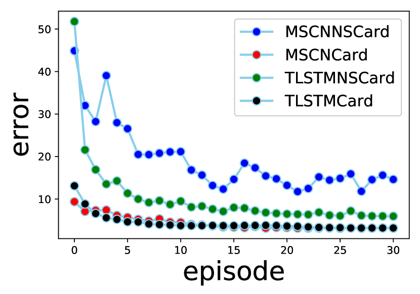
(a) Card Validation Error

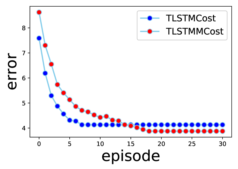
(b) Cost Validation Error

Figure 7: Validation Error on Numeric Workload

LSTM vs NN. On the JOB-light workload, TLSTMCard outperforms TNNCard by 3 times on max error for cardinality estimation and 2 times on the mean error. TLSTMMCost outperforms TNNMCost by 3 times on mean error and max error for cost estimation. On the Synthetic workload, TLSTMCard outperforms TNNCard on all the cardinality errors. On the Scale workload, tree-LSTM outperforms tree-NN on all the cardinality errors and cost errors. TLSTMCard outperforms TNNCard on harder queries for cardinality estimation, and TLSTMMCost outperforms TNNMCost on all the cost errors. These results show that LSTM can help the representation model to learn more robust representations for sub-plans, because the LSTM has an extra channel to avoid information vanishing for complex queries.

Multi-Learning vs Cost Only Learning. On the JOB-light workload, multitask technique can help the model to achieve 3 times improvement on 90-99th, mean and max error for cost estimation. On the Synthetic workload, TLSTMMCost outperforms TLSTMCost on all the cost errors. On the Scale workload, TLSTMMCost outperforms TLSTMCost by more than 2 times on max error for cost estimation. The reason is that multitask learning can improve the generalization ability of the model for complex queries.

In summary, sample bitmap, tree-structured model, LSTM, and multitask learning can improve the quality of cost and cardinality estimation.

6.3 Effectiveness on the JOB workload with both string and numeric predicates

Methods. Table 11 shows the methods tested on the JOB workload with string and numeric predicates. The String shows methods in Section 5 which use the string embedding technique, including embedding on rules generation strings and embedding only on string values in datasets.

Table 9: Methods on JOB workload (with strings)

Methods	Target	Represent	Predicate	Estimate	String
PGCard	Card	No	No	No	No
TLSTMHashCard	Card	LSTM	LSTM	MULT	Hash
TLSTMEmbNRCard	Card	LSTM	LSTM	MULT	Embed
TLSTMEmbRCard	Card	LSTM	LSTM	MULT	Rule+Embed
TPoolEmbRCard	Card	LSTM	Pool	MULT	Rule+Embed
PGCost	Cost	No	No	No	No
TLSTMHashMCost	Cost	LSTM	LSTM	MULT	Hash
TLSTMEmbNRMCost	Cost	LSTM	LSTM	MULT	Embed
TLSTMEmbRMCost	Cost	LSTM	LSTM	MULT	Rule+Embed
TPoolEmbRMCost	Cost	LSTM	Pool	MULT	Rule+Embed

Table 10: Cardinality errors on the JOB workload

Cardinality	median	90th	95th	99th	max	mean
PGCard	184	8303	34204	1.06e5	6.70e5	10416
TLSTMHashCard	11.1	207	359	824	1371	83.3
TLSTMEmbNRCard	11.6	181	339	777	1142	70.2
TLSTMEmbRCard	10.9	136	227	682	904	55.0
TPoolEmbRCard	10.1	74.7	193	679	798	47.5

Table 11: Cost errors on the JOB workload

Cost	median	90th	95th	99th	max	mean
PGCost	4.90	80.8	104	3577	4920	105
TLSTMHashMCost	4.47	53.6	149	239	478	24.1
TLSTMEmbNRMCost	4.12	18.1	44.1	105	166	10.3
TLSTMEmbRMCost	4.28	13.3	22.5	104	126	8.6
TPoolEmbRMCost	4.07	11.6	17.5	63.1	67.3	7.06

In order to investigate different techniques proposed in the paper effectively, we divide the training data into two parts and train on them respectively. The first is workload without join, and the second is workload with multiple joins. All these training queries contain complicated predicates on both numeric and string values, and they are generated randomly. Firstly, we train our models on the first workload and test them on single table validation workload, and this can compare the performance of different predicate embedding techniques directly. Secondly, we train our models on the second workload and evaluate them on 113 JOB queries, and this can compare the effects of different predicate embedding techniques on complicated queries estimation.

6.3.1 Evaluation on single table workload

The predicates in the workload contain string equal search, string pattern search, range query and numeric equal search. For conjunction predicates, the complex predicates are composed of expressions with ‘AND’ and ‘OR’ semantics. The most complex predicate in the workload has 4 boolean conjunctions and 5 expressions. We set the batch size as 64 and divide all 56,000 queries into 882 batches. We take the first 800 batches as the training data, and the remainders as validation data. We use the Adam optimizer and the learning rate is 0.001. Since the semantic of predicates doesn’t have much effect on execution cost on single table queries (Scan operation on the same table takes similar time no matter what predicate is.), we only report the validation error for cardinality estimation. The results are shown in Figure 8.

Hash Bitmap vs String Embedding. As shown in Figure 8, TLSTMHashCard performs the worst on validation queries and it converge speed is the slowest. TLSTMEmbNRCard outperforms TLSTMHashCard by 30%, because string embedding can capture coexistence relation among different strings to improve the performance on the validation workload.

Rule vs No-Rule. In Figure 8, TLSTMEmbRCard outperforms TLSTMEmbNRCard by around 15% on cardinality estimation, because the coverage of strings in the workload to be trained is different, and the rules are selected for covering more strings in the workload and the method with rule can pre-train many more strings and encode them with more accurate distributed representations.

Tree-Pooling Predicate vs Tree-LSTM Predicate. Both TLSTMEmbRCard and TPoolEmbRCard can make full use of string embedding, but they make difference in cardinality estimation (TPoolEmbRCard outperforms TLSTMEmbRCard by 20% on validation workload), because the tree structure with Min-Max pooling is more capable of representing compound predicate in semantic, and it can learn a better predicate representation with stronger generalization ability.

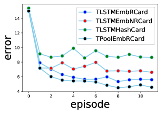
Figure 8: Cardinality Validation Error on A Single Table

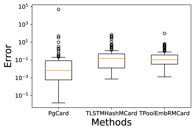
(a) Cardinality

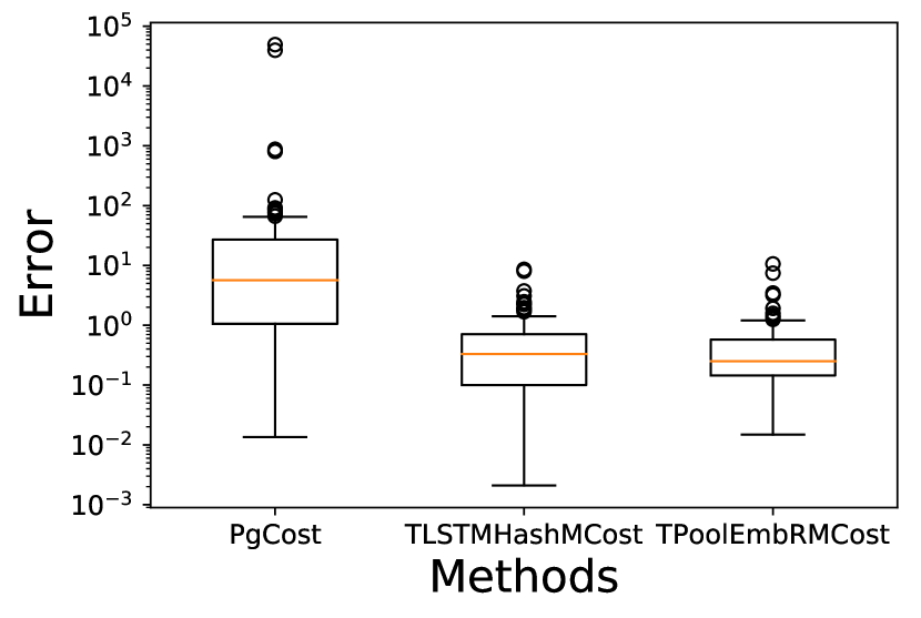
(b) Cost

Figure 9: Estimation errors on the JOB workload. The box boundaries are at the 25th/50th/75th percentiles

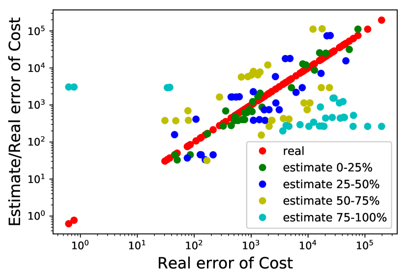
(a) PGCost

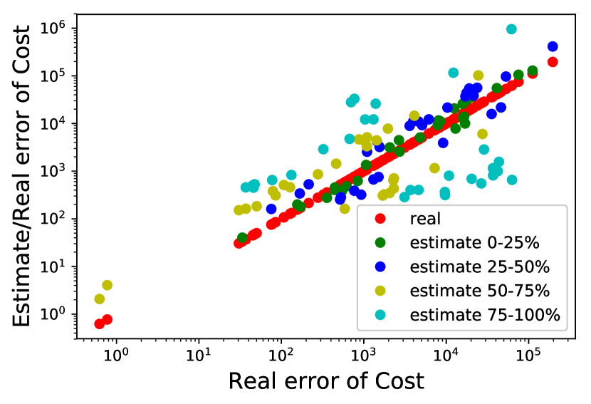
(b) TLSTMEmbNRMCost

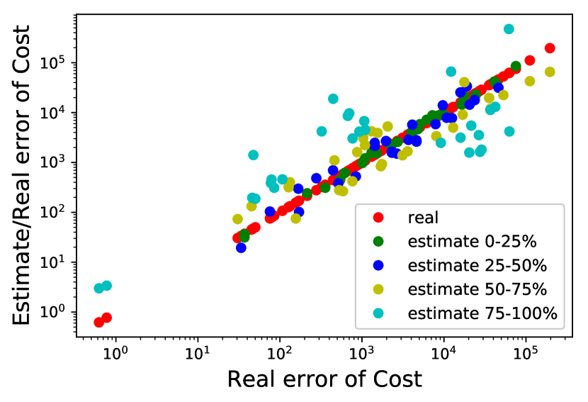
(c) TPoolEmbRMCost

Figure 10: Distribution of Estimated Cost

6.3.2 Evaluation on the JOB workload

We train the representation and output layers on 100,000 queries with multiple joins. We take 90% of multi-table join queries as training data and 10% of them as validation data. We train the model until the validation cardinality error will not decrease anymore, and then we evaluate the trained model on JOB queries. The results for cardinality estimation are shown in Table 11 and the results for cost estimation are shown in Table 11.

Hash Bitmap vs String Embedding. TLSTMEmbNRCard outperforms TLSTMHashCard on 90-99th errors, max error and mean error for cardinality estimation, because with highly representative of string embedding, the string embedding not only learns the correlations among columns but learns the correlations among tables, and thus the methods with string embedding perform well for cardinality estimation on complex queries with multiple joins. Moreover, the performance difference between TLSTMEmbNRMCost and TLSTMHashMCost is even larger. TLSTMEmbNRMCost outperforms TLSTMHashMCost by 2 times on mean and 99th errors, and 3 times on max, 95th and 90th errors. Similar to cardinality estimation, the improvement on complex queries in TLSTMEmbNRMCost is due to the correlations carried by string embedding.

Rule vs No-Rule. TLSTMEmbRCard outperforms TLSTMEmbNRCard on all the errors for cardinality estimation, especially on 90-99th errors, max error and mean error. The methods with rules achieve better performance, because the rules extract lots of substrings from datasets so that all the strings in the workload are trained and the distribution representations of strings contain more coexistence relations. Complex queries tend to gain more benefit from rules, because errors would accumulate rapidly for complex queries. Similar to cardinality estimation, TLSTMEmbRMCost outperforms TLSTMEmbNRMCost on 90-95th,max and mean errors.

Tree-Pooling Predicate vs Tree-LSTM Predicate. The difference between TLSTMEmbRCard and TPoolEmbRCard is the structure of the predicate embedding model, and TPoolEmbRCard outperforms TLSTMEmbRCard on all the cardinality errors and TPoolEmbRMCost outperforms TLSTMEmbRMCost on all the cost errors. This is because the tree model using the Min-Max Pooling can represent the compound predicate better and train a more robust model for cardinality and cost estimation. On 99th and max errors for cost estimation, TPoolEmbRMCost outperforms TLSTMEmbRMCost by 1.5-2 times, because the predicates representation trained by the Min-Max Pooling structure still keeps accurate for complex queries.

Distribution of errors. Figure 9 shows the error variance on the JOB workload. For PostgreSQL, we have tuned the factor of page IO so that the unit of the estimated cost equals to the unit of time (milliseconds here). However, it still overestimates the cost and underestimates the cardinality, and the maximal error is very large in both negative and positive sides. Our methods underestimate both cost and cardinality of queries, but errors of our methods are more concentrated and smaller. We adjust the unit of estimated cost to be the same as real execution time by using a factor for each method, and we draw the real time and estimated cost together in Figure 10, which is more intuitive and comprehensive. The cost estimated by TPoolEmbRMCost fits the real time very well. PGCost can not estimate the small cost at all and the estimated cost is very scattered. The error distribution of TLSTMHashMCost is between the TPoolEmbRMCost and PGCost.

In summary, the string embedding, using rules to embed the strings, and tree-pooling can improve the quality of cost and cardinality estimation.

6.4 Efficiency

Table 12 shows the efficiency of different methods on 113 queries on the JOB workload. The Batch indicates whether the batch technique described in Section 4.3 is used. The cost evaluation time of PostgreSQL is obtained from the planning time without query optimization. TLSTM and TPool estimate these queries one by one, and TLSTMBatch and TPoolBatch estimate these queries in batch.

Table 12: Efficiency Evaluation

Methods	Represent	Predicate	Estimate	Batch	Time(ms)
PostgreSQL	No	No	No	No	18.9
MSCN	No	No	SING	No	14.2
MSCNBatch	No	No	SING	Yes	6.28
TLSTM	LSTM	LSTM	MULT	No	70.3
TLSTMBatch	LSTM	LSTM	MULT	Yes	7.79
TPool	LSTM	Pool	MULT	No	47.3
TPoolBatch	LSTM	Pool	MULT	Yes	3.63

Batch vs No-Batch. TPoolBatch outperforms TPool by one order of magnitude, TLSTMBatch also outperforms TLSTM by one order of magnitude. This is because that the batch evaluation reduces the number of times computing the model in nodes of the trees, and increases the parallelism as discussed in Section 4.3.

Tree-Pooling Predicate vs Tree-LSTM Predicate. TPool outperforms TLSTM by 50%, and TPoolBatch outperforms TLSTMBatch by 2 times. This is because tree-pooling replaces some neural networks in the predicate model, and thus has less computation cost in estimation.

7 Conclusion

In this paper, we proposed an end-to-end learning-based tree-structured cost estimator for estimating both cost and cardinality. We encoded query operation, meta data, query predicate and some samples into the model. The model contained embedding layer, representation layer and estimation layer. We proposed an effective method to encode string values into the model to improve the model generalization. Extensive results on real datasets showed that our method outperformed existing techniques.

References

- [1] Db2. https://en.wikipedia.org/wiki/IBM_Db2_Family.
- [2] Postgresql. https://www.postgresql.org/.
- [3] Set cover problem. https://en.wikipedia.org/wiki/Set_cover_problem, 2014.
- [4] M. Akdere, U. Çetintemel, M. Riondato, E. Upfal, and S. B. Zdonik. Learning-based query performance modeling and prediction. In ICDE, pages 390–401, 2012.
- [5] R. Caruana. Multitask learning. Machine Learning, 28(1):41–75, 1997.
- [6] M. Durand and P. Flajolet. Loglog counting of large cardinalities. In Algorithms - ESA, pages 605–617, 2003.
- [7] P. Flajolet and G. N. Martin. Probabilistic counting algorithms for data base applications. Journal of Computer and System Sciences, 31(2):182 – 209, 1985.
- [8] P. Flajolet, Éric Fusy, O. Gandouet, and et al. Hyperloglog: The analysis of a near-optimal cardinality estimation algorithm. In AOFA, 2007.
- [9] A. Ganapathi, H. Kuno, U. Dayal, J. L. Wiener, A. Fox, M. Jordan, and D. Patterson. Predicting multiple metrics for queries: Better decisions enabled by machine learning. In ICDE, pages 592–603, 2009.
- [10] F. Giroire. Order statistics and estimating cardinalities of massive data sets. Discrete Applied Mathematics, 157(2):406 – 427, 2009.
- [11] S. Gulwani. Automating string processing in spreadsheets using input-output examples. In T. Ball and M. Sagiv, editors, POPL, pages 317–330, 2011.
- [12] S. Gulwani, W. R. Harris, and R. Singh. Spreadsheet data manipulation using examples. Commun. ACM, 55(8):97–105, 2012.
- [13] Y. E. Ioannidis. The history of histograms (abridged). In J. C. Freytag, P. C. Lockemann, S. Abiteboul, M. J. Carey, P. G. Selinger, and A. Heuer, editors, PVLDB, pages 19–30, 2003.
- [14] A. Kipf, T. Kipf, B. Radke, V. Leis, P. A. Boncz, and A. Kemper. Learned cardinalities: Estimating correlated joins with deep learning. In CIDR, 2019.
- [15] V. Leis, A. Gubichev, A. Mirchev, P. A. Boncz, A. Kemper, and T. Neumann. How good are query optimizers, really? PVLDB, 9(3):204–215, 2015.
- [16] V. Leis, B. Radke, A. Gubichev, A. Kemper, and T. Neumann. Cardinality estimation done right: Index-based join sampling. In CIDR, 2017.
- [17] J. Li, A. C. König, V. Narasayya, and S. Chaudhuri. Robust estimation of resource consumption for sql queries using statistical techniques. PVLDB, 5(11):1555–1566, July 2012.
- [18] R. J. Lipton, J. F. Naughton, and D. A. Schneider. Practical selectivity estimation through adaptive sampling. SIGMOD Rec., 19(2):1–11, May 1990.
- [19] F. Liu and S. Blanas. Forecasting the cost of processing multi-join queries via hashing for main-memory databases. In SoCC, pages 153–166, 2015.
- [20] G. Lohman. Is query optimization a "solved" problem?, 2014.
- [21] T. Malik, R. C. Burns, and N. V. Chawla. A black-box approach to query cardinality estimation. In CIDR, pages 56–67, 2007.
- [22] R. Marcus and O. Papaemmanouil. Plan-structured deep neural network models for query performance prediction. CoRR, abs/1902.00132, 2019.
- [23] T. Mikolov, I. Sutskever, K. Chen, G. S. Corrado, and J. Dean. Distributed representations of words and phrases and their compositionality. In C. J. C. Burges, L. Bottou, Z. Ghahramani, and K. Q. Weinberger, editors, NIPS, pages 3111–3119, 2013.
- [24] T. Neumann, V. Leis, and A. Kemper. The complete story of joins (in hyper). In BTW, pages 31–50, 2017.
- [25] F. Olken and D. Rotem. Random sampling from database files: A survey. In Statistical and Scientific Database Management, 1990.
- [26] J. Ortiz, M. Balazinska, J. Gehrke, and S. S. Keerthi. Learning state representations for query optimization with deep reinforcement learning. In DEEM@SIGMOD, pages 4:1–4:4, 2018.
- [27] K. Whang, B. T. V. Zanden, and H. M. Taylor. A linear-time probabilistic counting algorithm for database applications. ACM Trans. Database Syst., 15(2):208–229, 1990.
- [28] W. Wu, Y. Chi, S. Zhu, J. Tatemura, H. Hacigümüs, and J. F. Naughton. Predicting query execution time: Are optimizer cost models really unusable? In ICDE, pages 1081–1092, April 2013.
- [29] W. Wu, J. F. Naughton, and H. Singh. Sampling-based query re-optimization. In SIGMOD, pages 1721–1736, 2016.
- [30] N. Zhang, P. J. Haas, V. Josifovski, G. M. Lohman, and C. Zhang. Statistical learning techniques for costing xml queries. In PVLDB, pages 289–300, 2005.