Assouad spectrum thresholds for some random constructions

Abstract.

The Assouad dimension of a metric space determines its extremal scaling properties. The derived notion of the Assouad spectrum fixes relative scales by a scaling function to obtain interpolation behaviour between the quasi-Assouad and box-counting dimensions. While the quasi-Assouad and Assouad dimensions often coincide, they generally differ in random constructions. In this paper we consider a generalised Assouad spectrum that interpolates between the quasi-Assouad to the Assouad dimension. For common models of random fractal sets we obtain a dichotomy of its behaviour by finding a threshold function where the quasi-Assouad behaviour transitions to the Assouad dimension. This threshold can be considered a phase transition and we compute the threshold for the Gromov boundary of Galton-Watson trees and one-variable random self-similar and self-affine constructions. We describe how the stochastically self-similar model can be derived from the Galton-Watson tree result.

1. Introduction

The Assouad dimension is an important notion in embedding theory due to the famous Assouad embedding theorem [Ass77, Ass79], which implies that a metric space $X$ cannot be embedded by a bi-Lipschitz map into $\operatorname{\mathbb{R}}^{d}$ for any $d$ less than the Assouad dimension of $X$. The Assouad dimension is therefore a good indicator of thickness in a metric space and is an upper bound to most notions of dimensions in use today [Fra14, Rob11]. In particular, it is an upper bound to the Hausdorff, box-counting, and packing dimension. Heuristically, the Assouad dimension “searches” for the thickest part of a space relative to two scales $0<r<R$ by finding the minimal exponent $s$ such that the every $R$-ball can be covered by at most $(R/r)^{s}$ balls of diameter $r$.

Over the last few years much progress has been made towards our understanding of this dimension and it is now a crucial part of fractal geometry, see e.g. [Che19, Fra14, FMT18, GHM16, KR16, Tro19] and references therein. Several other notions of dimension were derived from its definition and this family of Assouad-type dimensions has attracted much interest. An important notion is the $\theta$-Assouad spectrum introduced by Fraser and Yu [FY18] which aims to interpolate between the upper box-counting and the Assouad dimension to give fine information on the structure of metric spaces, see [Fra19] for a recent survey. It analyses sets by fixing the relation $r=R^{1/\theta}$ in the definition of the Assouad dimension for parameters $\theta\in(0,1)$.

It turns out that the Assouad spectrum interpolates between the upper box-counting dimension and the quasi-Assouad dimension introduced by Lü and Xi [LX16]. That is, for $\theta\to 0$ the $\theta$-Assouad spectrum tends to the upper box-counting dimension, whereas for $\theta\to 1$ it approaches the quasi-Assouad dimension, see [FHH+19]. In fact, the quasi-Assouad could be defined in terms of the Assouad spectrum.

In many cases the quasi-Assouad dimension and Assouad dimension coincide and the Assouad spectrum gives best relative scaling information. However, in many stochastic settings they differ. This can be explained by the Assouad dimension picking up very extreme behaviour that is almost surely lost over all geometric scales [FMT18].

In their landmark paper [FY18], Fraser and Yu discuss the possibility of extending the definition of the Assouad spectrum to analyse the case when quasi-Assouad and Assouad dimension differ. These general spectra, which we shall also refer to as generalised Assouad spectra, would then shed some line on the behaviour of ‘in-between’ scales. This is done by changing the relation $r=R^{1/\theta}$ to a general dimension function $r=\varphi(R)$. García, Hare and Mendivil studied this notion of spectrum (including their natural dual: the lower Assouad dimension spectrum) and obtain similar interpolation results as are the case for the Assouad spectrum, see [GHM19]. A common observation is that the intermediate spectrum is constant and equal to either the quasi-Assouad or Assouad dimension around a threshold function. That is, there exists a function $\phi(x)$ such that $\operatorname{{\dim}_{\mathrm{A}}^{\,\varphi}}F=\operatorname{\dim_{\,\mathrm{qA}}}F$ for $\operatorname{\varphi}(x)=\upomega(\phi(x))$ and $\operatorname{{\dim}_{\mathrm{A}}^{\,\varphi}}F=\operatorname{\dim_{\mathrm{A}}}F$ for $\operatorname{\varphi}(x)=o(\phi(x))$, where we have used the standard little omega- and $o$-notation. The standard examples where quasi-Assouad and Assouad dimensions differ are random constructions and this threshold can be considered a phase transition in the underlying stochastic process. In this paper we will explore this threshold function for various random models.

García et al. [GHM19a] considered the following random construction: Let $(l_{i})$ be a non-increasing sequence such that $\sum l_{i}=1$. For each $i$, let $U_{i}$ be an i.i.d. copy of $U$, the random variable that is uniformly distributed in $[0,1]$. Note that, almost surely $U_{i}\neq U_{j}$ for all $i\neq j$. Therefore, almost surely, there is a total ordering of the $(U_{i})$. The complementary set of the random arrangement $E$ is defined as the complement of arranging open intervals of length $l_{i}$ in the order induced by $(U_{i})$. That is,

$$E=\bigcup_{y\in[0,1]}\left\{x=\sum_{V_{y}}l_{i}\;:\;V_{y}=\{i:U_{i}<y\}\right\}.$$

Almost surely, this set in uncountable and has a Cantor-like structure. García et al. have previously determined the (quasi-)Assouad dimension of deterministic realisations [GHM16], where the order is taken as $U_{i}<U_{i+1}$ as well as the Cantor arrangement, when $U_{i}$ is equal to the right hand end point of the canonical construction intervals of the Cantor middle-third set (ignoring repeats). They confirmed in [GHM19a] that the quasi-Assouad dimension of $E$ is almost surely equal to the quasi-Assouad dimension of the Cantor arrangement $C$, whereas the Assouad dimension takes the value $1$. They further gave the threshold function, which they computed as $\phi(x)=\log|\log x|/|\log x|$.

Theorem 1.1 (García et al. [GHM19a]).

Let $\phi(x)=\log|\log x|/|\log x|$ and $l_{i}$ be a decreasing sequence such that $\sum l_{i}=1$. Assume further that there exists $\operatorname{\varepsilon}>0$ such that

$$\operatorname{\varepsilon}<\frac{\sum_{j\geq 2^{n+1}}l_{j}}{\sum_{j\geq 2^{n}}l_{j}}<1-\operatorname{\varepsilon}.$$

Then, almost surely, $\operatorname{{\dim}_{\mathrm{A}}^{\,\varphi}}E=\operatorname{{\dim}_{\mathrm{A}}^{\,\varphi}}C$ for $\operatorname{\varphi}=\upomega(\phi(x))$ and $\operatorname{{\dim}_{\mathrm{A}}^{\,\varphi}}E=1$ for $\operatorname{\varphi}=o(\phi(x))$.

In this article we give elementary proofs of the threshold dimension functions for several canonical random sets. Under separation conditions we obtain the threshold for one-variable random iterated function systems with self-similar maps and self-affine maps of Bedford-McMullen type. We also determine the threshold for the Gromov boundary of Galton-Watson trees. While we do not state it explicitly, using the methods found in [Tro19], our results for Galton-Watson trees directly applies to stochastically self-similar and self-conformal sets as well as fractal percolation sets.

Our proofs rely on the theory of large deviations as well as a dynamical version of the Borel-Cantelli lemmas.

2. Definitions and Results

Let $\phi:\operatorname{\mathbb{R}}^{+}\to\operatorname{\mathbb{R}}^{+}$. We say that $\phi$ is a dimension function if $\phi(x)$ and $\phi(x)|\log x|$ are monotone. Let $N_{r}(X)$ be the minimal number of sets of radius at most $r$ needed to cover $X$. The generalised Assouad spectrum (or intermediate Assouad spectrum) with respect to $\phi$ is given by

$$\operatorname{{\dim}_{\mathrm{A}}^{\phi}}F=\inf\bigg{\{}s\;:\;(\exists C>0)(\forall 0<r=R^{1+\phi(R)}<R<1)\\ \sup_{x\in F}N_{r}(F\cap B(x,R))\leq C\left(\frac{R}{r}\right)^{s}=R^{-\phi(R)s}\bigg{\}}.$$

We will also refer to this quantity as the $\phi$-Assouad dimension of $F$. Many other variants of the Assouad dimension can now be obtained by restricting $\phi$ in some way: The Assouad spectrum $\operatorname{{\dim}_{\mathrm{A}}^{\,\theta}}$ considered by Fraser and Yu can be obtained by setting $\phi(R)=1/\theta-1$. The quasi-Assouad dimension $\operatorname{\dim_{\,\mathrm{qA}}}F$ is given by the limit $\operatorname{\dim_{\,\mathrm{qA}}}F=\lim_{\theta\to 1}\operatorname{{\dim}_{\mathrm{A}}^{\,\theta}}F$, whereas the Assouad dimension is obtained by letting $\phi(R)=0$ and allowing $r\leq R$. We note that we define the generalised Assouad spectrum slightly differently than in [FY18]. Instead of requiring $r=\varphi(R)$, we consider the dimension function $\phi$ setting $r=R^{1+\phi(R)}$. Hence, $\varphi(R)/R=R^{\phi(R)}$. We use this notation as it is slightly more convenient to use.

In fractal geometry two canonical models are used to obtain random fractal sets: stochastically self-similar sets and one-variable random sets. Instead of computing the result for stochastically self-similar sets, we compute it for Galton-Watson processes from which the stochastically self-similar case will follow. We will then move on to one-variable random constructions and analyse random self-similar constructions, as well as a randomisation of Bedford-McMullen carpets.

2.1. Galton-Watson trees and stochastically self-similar sets

Let $X$ be a random variable that takes values in $\{0,\cdots,N\}$ and write $\theta_{j}=\operatorname{\mathbb{P}}\{X=j\}$ for the probability that $X$ takes value $j$. The Galton-Watson process $Z_{i}$ is defined inductively by letting $Z_{0}=1$ and $Z_{k+1}=\sum_{j=1}^{Z_{k}}X_{j}$, where each summand $X_{j}$ is an i.i.d. copy of $X$. The Galton-Watson tree is obtained by considering a tree with single root and determining ancestors for every node with law $X$, independent of all other nodes. The number of nodes at level $k$ is then given by $Z_{k}$ and, conditioned on non-extinction, this process generates a (random) infinite tree. We endow the set of infinite descending paths starting at the root with the standard metric $d(x,y)=2^{-\lvert x\wedge y\rvert}$, where $\lvert x\wedge y\rvert$ is the level of the least common ancestor. This gives rise to the Gromov boundary of the random tree that we refer to as $F_{\tau}$.

Throughout, we assume that we are in the supercritical case, i.e.

$$m=\operatorname{\mathbb{E}}(X)=\sum_{k=1}^{N}\theta_{k}k>1.$$

The normalised Galton-Watson process is defined by $W_{k}=Z_{k}/m^{k}$. It is a standard application of the martingale convergence theorem to show that $W_{k}\to W$ almost surely. Conditioned on non-extinction we additionally have $W\in(0,\infty)$ almost surely. We refer the reader to [Liu00] and [LPP95] for some other fundamental dimension theoretic results of Galton-Watson processes.

It was established in [FMT18] that the Gromov boundary, using the standard metric, has Assouad dimension $\log N/\log 2$ almost surely. In [Tro19], the quasi-Assouad dimension was computed as

$$\operatorname{\dim_{\,\mathrm{qA}}}F_{\tau}=\frac{\log\operatorname{\mathbb{E}}(X)}{\log 2}=\operatorname{\dim_{\mathrm{B}}}F_{\tau}=\operatorname{\dim_{\mathrm{H}}}F_{\tau}$$

almost surely. This means, in particular, that the $\theta$-Assouad spectrum is constant and equal to the Hausdorff dimension. This is in fact the typical behaviour for all dimension functions $\phi(x)\leq C(\log|\log x|/|\log x|)$, where $C>0$ is some constant. Conversely, for $\phi(x)=\upomega(\log|\log x|)/|\log x|)$ we recover the Assouad dimension, c.f. Theorem 1.1.

Theorem 2.1.

Let $F_{\tau}$ be the Gromov boundary of a supercritical Galton-Watson tree with bounded offspring distribution. Let

$$\phi(x)>\frac{\log|\log x|}{|\log x|}(\varepsilon\log m)^{-1}$$

be a dimension function. Then

$$\operatorname{{\dim}_{\mathrm{A}}^{\phi}}F_{\tau}\leq(1+\varepsilon)\operatorname{\dim_{\mathrm{B}}}F_{\tau}$$

almost surely.

Note that we trivially have $\operatorname{{\dim}_{\mathrm{A}}^{\phi}}F\geq\operatorname{\dim_{\mathrm{B}}}F$ and so

Corollary 2.2.

Let $\phi(x)=\upomega(\log|\log x|/|\log x|)$ be a dimension function. Then $\operatorname{{\dim}_{\mathrm{A}}^{\phi}}F_{\tau}=\operatorname{\dim_{\mathrm{B}}}F_{\tau}=\operatorname{\dim_{\mathrm{H}}}F_{\tau}$ almost surely.

For the reverse direction we obtain the following bound.

Theorem 2.3.

Let $F_{\tau}$ be the Gromov boundary of a supercritical Galton-Watson tree with bounded offspring distribution. Let $N$ be the maximal integer s.t. $\theta_{N}>0$. Further, let

$$\phi(x)<\frac{\log|\log x|}{|\log x|}\frac{\log(N/m)}{\varepsilon\log m\log N}.$$ (2.1)

be a dimension function. Then, almost surely,

$$\operatorname{{\dim}_{\mathrm{A}}^{\phi}}F_{\tau}\geq\min\{(1+\varepsilon)\operatorname{\dim_{\mathrm{B}}}F_{\tau},\operatorname{\dim_{\mathrm{A}}}F_{\tau}\}.$$

almost surely.

Assume that $m<N$ and so $\operatorname{\dim_{\mathrm{B}}}F_{\tau}<\operatorname{\dim_{\mathrm{A}}}F_{\tau}$ almost surely. Then, for $\varepsilon$ satisfying $(1+\varepsilon)=\operatorname{\dim_{\mathrm{A}}}F/\operatorname{\dim_{\mathrm{B}}}F=\log N/m$, we obtain $\operatorname{{\dim}_{\mathrm{A}}^{\phi}}F_{\tau}\geq\operatorname{\dim_{\mathrm{A}}}F_{\tau}$ almost surely. It follows that for

$$\phi(x)<\frac{\log|\log x|}{\log(1/x)}\frac{\log(N/m)}{(N/m)\log m\log N}=\frac{m}{N}\left(\frac{1}{\log m}-\frac{1}{\log N}\right)\frac{\log|\log x|}{|\log x|}$$

we get $\operatorname{{\dim}_{\mathrm{A}}^{\phi}}F=\operatorname{\dim_{\mathrm{A}}}F$.

Corollary 2.4.

There exists $C>0$ such that, almost surely, $\operatorname{{\dim}_{\mathrm{A}}^{\phi}}F_{\tau}=\operatorname{\dim_{\mathrm{A}}}F_{\tau}$ for all dimension functions $\phi(x)\leq C\log|\log x|/|\log x|)$.

We will prove both theorems in Section 3. These two bounds are not optimal in the sense that there is a slight gap between the upper and the lower bound. This gap, after rearranging, is of order $1-\log m/\log N=1-\operatorname{\dim_{\mathrm{B}}}F/\operatorname{\dim_{\mathrm{A}}}F$. Let $\phi_{\varepsilon}$ be equal to the right hand side of (2.1). We can combine Theorems 2.1 and 2.3 to give

$$(1+\varepsilon)\operatorname{\dim_{\mathrm{B}}}F\leq\dim_{\textrm{A}}^{\phi_{\varepsilon}}F\leq(1+\varepsilon)\frac{\operatorname{\dim_{\mathrm{A}}}F}{\operatorname{\dim_{\mathrm{A}}}F-\operatorname{\dim_{\mathrm{B}}}F}\operatorname{\dim_{\mathrm{B}}}F$$

for an appropriate range of $\varepsilon>0$.

2.1.1. Stochastically self-similar sets

This result can also be applied in the setting of stochastically self-similar sets that were first studied by Falconer [Fal86] and Graf [Gra87]. Since we do not exclude the case where there is no descendant, the analysis also applies to fractal percolation in the sense of Falconer and Jin [FJ15]. In the case of Mandelbrot percolation, where a $d$-dimensional cube is split into $n^{d}$ equal subcubes of sidelength $1/n$ and is kept with probability $p>0$, the number of subcubes is a Galton-Watson process and the surviving subcubes at level $k$ can be modelled by a Galton-Watson tree. Since subcubes at the same level have the same diameters, the limit set is almost surely bi-Lipschitz to the Gromov boundary of an appropriately set up Galton-Watson tree with the small caveat that the graph metric need to be changed from $d(x,y)=2^{-|x\wedge y|}$ to $d^{\prime}(x,y)=n^{|-x\wedge y|}$. This change, however, just affects the results above by a constant and not their asymptotic behaviour. For non-homogeneous self-similar sets, where the size may vary at a given generation, one needs to set up a Galton-Watson tree that models the set. This is described in full detail in [Tro19] and we omit its full derivation for this model here. Using those methods, Theorems 2.1 and 2.3 become the following corollary.

Corollary 2.5.

Let $F_{\tau}$ be a stochastically self-similar set arising from finitely many self-similar IFS that satisfy the uniform open set condition. Then, if $\phi(x)=\upomega(\log|\log x|/|\log x|)$, we obtain $\operatorname{{\dim}_{\mathrm{A}}^{\phi}}F_{\tau}=\operatorname{\dim_{\mathrm{B}}}F_{\tau}$ almost surely. Conversely, if $\phi(x)=o(\log|\log x|/|\log x|)$, then $\operatorname{{\dim}_{\mathrm{A}}^{\phi}}F_{\tau}=\operatorname{\dim_{\mathrm{A}}}F_{\tau}$.

2.2. One-variable random sets

A different popular model for random fractal sets is the one-variable model. It is sometimes also referred to as a homogeneously random construction. We will avoid the latter term to avoid ambiguity with homogeneous iterated function systems. Let $\Lambda\subset\operatorname{\mathbb{R}}^{n}$ be a compact set supporting the Borel-probability measure $\mu$. For each $\lambda\in\Lambda$ we associate an iterated function system $\mathbb{I}_{\lambda}=\{f^{\lambda}_{1},\dots,f^{\lambda}_{N_{\lambda}}\}$, where each $f_{i}^{\lambda}$ is a strictly contracting diffeomorphism on some non-empty open set $V$. Throughout this section we make the standing assumption that $\sup_{\lambda}N_{\lambda}<\infty$, that $0<\inf_{\lambda,i,x}\lvert(f_{i}^{\lambda})^{\prime}(x)\rvert\leq\sup_{\lambda,i,x}\lvert(f_{i}^{\lambda})^{\prime}(x)\rvert<1$, and that there exists a non-empty compact set $\Delta\subset V$ such that $f_{i}^{\lambda}(\Delta)\subseteq\Delta$ for all $\lambda\in\Lambda$ and $1\leq i\leq N_{\lambda}$. To each $\omega\in\Omega=\Lambda^{\operatorname{\mathbb{N}}}$, we associate the set $F_{\omega}$ given by

$$F_{\omega}=\bigcap_{k=1}^{\infty}\;\bigcup_{\begin{subarray}{c}1\leq i_{j}\leq N_{\lambda_{j}}\\ 1\leq j\leq k\end{subarray}}f_{i_{k}}^{\lambda_{k}}\circ\dots\circ f_{i_{1}}^{\lambda_{1}}(\Delta).$$

Let $\operatorname{\mathbb{P}}=\mu^{(\operatorname{\mathbb{N}})}$ be the product measure on $\Omega=\Lambda^{\operatorname{\mathbb{N}}}$. We write

$$\operatorname{\mathbb{E}}(X(\omega))=\int_{\Omega}X(\omega)d\operatorname{\mathbb{P}}(\omega)\quad\text{and}\quad\operatorname{\mathbb{E}}^{g}(X(\omega))=\exp\int_{\Omega}\log X(\omega)d\operatorname{\mathbb{P}}(\omega)$$

The one-variable random attractor $F_{\omega}$ is then obtained by choosing $\omega\in\Omega$ according to the law $\operatorname{\mathbb{P}}$.

2.2.1. One-variable random self-similar sets

To make useful dimension estimates we have to restrict the class of functions. The simplest model is that of self-similar sets, where we restrict $f_{i}^{\lambda}$ to similarities. That is, $\lvert f_{i}^{\lambda}(x)-f_{i}^{\lambda}(y)\rvert=c_{i}^{\lambda}\lvert x-y\rvert$ for all $x,y\in V$ and some $c_{i}^{\lambda}>0$. It is well-known that for self-similar maps and our standing assumptions, the Hausdorff and box-counting dimensions are bounded above by the unique $s$ satisfying

$$\operatorname{\mathbb{E}}^{g}\left(\sum_{1\leq i\leq N_{\omega_{1}}}(c_{i}^{\omega_{1}})^{s}\right)=1.$$ (2.2)

If one further assumes that there exists a non-empty open set $U$ such that the union $\bigcup_{i=1}^{N_{\lambda}}f_{i}^{\lambda}(U)$ is disjoint for all $\lambda$ and $f_{i}^{\lambda}(U)\subseteq U$ we say that the uniform open set condition holds. Under this assumption the unique $s$ in (2.2) coincides with the Hausdorff, box-counting, and quasi-Assouad dimension of $F_{\omega}$ for $\operatorname{\mathbb{P}}$-almost all $\omega$, see e.g. [Tro17] and references therein. Since we refer to the sum above quite frequently we write $\operatorname{\mathfrak{S}}_{\lambda}^{t}=\sum(c_{i}^{\lambda})^{t}$. To avoid the trivial case when the Assouad dimension coincides with the Hausdorff dimension, and there is nothing to prove as the generalised Assouad dimension coincides with this common value, we make the assumption that the systems is not almost deterministic. That is, $\operatorname{\mathbb{P}}(\operatorname{\mathfrak{S}}_{\omega_{1}}^{s}=1)\neq 1$, where $s$ is the almost sure Hausdorff dimension. In particular, this implies that the Assouad dimension is strictly bigger than the Hausdorff (and upper box-counting) dimension. In fact, the Assouad dimension of $F_{\omega}$ is, almost surely, given by

$$\operatorname{\dim_{\mathrm{A}}}F_{\omega}=\sup\{s\;:\;\mu(\{\lambda\in\Lambda\;:\;\operatorname{\mathfrak{S}}_{\lambda}^{s}\geq 1\})>0\}$$

see [FMT18, Tro17]. To not obscure the result with needless technicality, we only analyse the case when the iterated function systems are homogeneous, i.e. $c_{i}^{\lambda}=c_{j}^{\lambda}$ for all $\lambda$. We write $c(\lambda)$ for the common value, then $\operatorname{\mathfrak{S}}_{\lambda}^{s}=N_{\lambda}c(\lambda)^{s}$.

Theorem 2.6.

Let $F_{\omega}$ be a one-variable random self-similar set generated by homogeneous iterated functions systems satisfying the uniform open set condition. Then the following dichotomy holds: Let $\phi(x)$ be a dimension function such that

$$\sum_{k=1}^{\infty}e^{-\phi(e^{-k})k}<\infty.$$

Then $\operatorname{{\dim}_{\mathrm{A}}^{\,\varphi}}F_{\omega}=\operatorname{\dim_{\mathrm{B}}}F_{\omega}$ for dimension functions $\operatorname{\varphi}(x)=\upomega(\phi(x))$, almost surely.

Conversely, let $\phi(x)$ be a dimension function such that

$$\sum_{k=1}^{\infty}e^{-\phi(e^{-k})k}=\infty.$$

Then $\operatorname{{\dim}_{\mathrm{A}}^{\,\varphi}}F_{\omega}=\operatorname{\dim_{\mathrm{A}}}F_{\omega}$ for dimension functions $\operatorname{\varphi}(x)=o(\phi(x))$, almost surely. Additionally, assume there exists $\Lambda^{\prime}\subset\Lambda$ such that $\operatorname{\mathfrak{S}}_{\lambda}^{s_{A}}=1$ for all $\lambda\in\Lambda^{\prime}$, where $s_{A}$ is the almost sure Assouad dimension of $F_{\omega}$, and $\mu(\Lambda^{\prime})>0$. Then the above result holds for all $\varphi(x)\leq C(\phi(x))$, where $C>0$ is some constant.

We prove this in Section 4. The methods we have used rely on the individual iterated function systems being homogeneous but we need not have made this argument. One can construct a subtree such that for this random realisation the covering numbers are comparable. Since this is somewhat more technical, we leave this case open.

2.2.2. One-variable random Bedford-McMullen carpets

Bedford-McMullen carpets are simple self-affine iterated function systems that are often the easiest to give as counterexamples to the self-similar theory [Bed84, McM84]. They consist of non-overlapping images of the unit square with fixed horizontal and vertical contraction of $1/m$ and $1/n$, respectively that align in an $m\times n$ grid of the unit square, see Figure 1 for two examples.

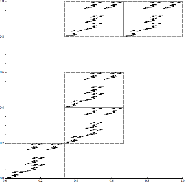
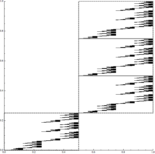
Figure 1. Two Bedford-McMullen carpets with their generating affine maps. The left example $F_{1}$ has $m_{1}=3$, $n_{1}=5$, $C_{1}=3$, $B_{1}=3$, and $N_{1}=5$. The right example $F_{2}$ has $m_{2}=2$, $n_{2}=4$, $C_{2}=3$, $B_{2}=2$, and $N_{2}=4$.

We randomise the construction in the same one-variable random fashion by choosing different sub rectangles at every step from the finite collection of possible arrangements. We denote these in the same way and write $2\leq m_{\lambda}<n_{\lambda}\leq N<\infty$ for the subdivisions. Then, $f_{i}^{\lambda}(x)$ are of the form

$$f_{i}^{\lambda}(x)=\begin{pmatrix}1/m_{\lambda}&0\\ 0&1/n_{\lambda}\end{pmatrix}x+\begin{pmatrix}a_{i}^{\lambda}\\ b_{i}^{\lambda}\end{pmatrix}$$

where $a_{i}^{\lambda}\in\{0,\dots,m_{\lambda}-1\}$ and $b_{i}^{\lambda}\in\{0,\dots,n_{\lambda}-1\}$. The boundedness of $n_{\lambda}$ implies that there are only finitely many IFSs with finitely many maps. Hence $\Lambda$ is finite and $\mu$ is finitely supported. We write $p_{\lambda}=\mu(\lambda)$.

We heavily rely on results in [FT18], where the $\theta$-Assouad spectrum of these attractors are found. In fact, this part can be considered an extension of [FT18], in the sense that the previous work gave a complete characterisation of the spectrum between the upper box-counting and the quasi-Assouad dimension, whereas we extend this to the Assouad dimension. Let $C_{\lambda}$ be the maximal number of maps that align in a column and $B_{\lambda}$ be the maximal number of non-empty columns. Further, let $N_{\lambda}$ be the number of maps in the IFS indexed by $\lambda$. See also Figure 1 for an example. Write $\overline{n}=\operatorname{\mathbb{E}}^{g}(n_{\lambda})$ and $\overline{m}=\operatorname{\mathbb{E}}^{g}(m_{\lambda})$. Similarly, let $\overline{B},\overline{C}$, and $\overline{N}$ denote their respective geometric means. The almost sure Assouad spectrum was found in [FT18] to be

$$\operatorname{{\dim}_{\mathrm{A}}^{\,\theta}}F_{\omega}=\begin{cases}\dfrac{1}{1-\theta}\left(\dfrac{\log\left(\overline{B}\,\overline{C}^{\theta}\overline{N}^{-\theta}\right)}{\log\overline{m}}+\dfrac{\log\left(\overline{N}\,\overline{B}^{-1}\overline{C}^{-\theta}\right)}{\sum_{\lambda}p_{\lambda}\log n_{\lambda}}\right),&0<\theta\leq\dfrac{\log\overline{m}}{\log\overline{n}};\\ \dfrac{\log\overline{B}}{\log\overline{m}}+\dfrac{\log\overline{C}}{\log\overline{n}},&\dfrac{\log\overline{m}}{\log\overline{n}}<\theta<1\,.\end{cases}$$

From this we can further deduce that

$$\operatorname{\dim_{\mathrm{B}}}F_{\omega}=\dfrac{\log\overline{B}}{\log\overline{m}}+\dfrac{\log\overline{N}\,\overline{B}^{-1}}{\log\overline{n}}\quad\text{ and }\quad\operatorname{\dim_{\,\mathrm{qA}}}=\frac{\log\overline{B}}{\log\overline{m}}+\frac{\log\overline{C}}{\log\overline{n}}.$$

However, the almost sure Assouad dimension is generally distinct from the quasi-Assouad dimension and given by

$$\operatorname{\dim_{\mathrm{A}}}F_{\omega}=\max_{\lambda\in\Lambda}\,\frac{\log B_{\lambda}}{\log m_{\lambda}}\,+\,\max_{\lambda\in\Lambda}\,\frac{\log C_{\lambda}}{\log n_{\lambda}}.$$

see [FMT18]. Note, in particular, that the dimension does not depend on the exact form of $\mu$, provided it is supported on $\Lambda$. Our main result in this section is bridging this gap with a similar dichotomy as for self-similar sets.

Theorem 2.7.

Let $F_{\omega}$ be a one-variable random Bedford-McMullen carpet. Then the following dichotomy holds: Let $\phi(x)\leq\log\overline{n}/\log\overline{m}-1$ be a dimension function such that

$$\sum_{k=1}^{\infty}e^{-\phi(e^{-k})k}<\infty.$$

Then $\operatorname{{\dim}_{\mathrm{A}}^{\,\varphi}}F_{\omega}=\operatorname{\dim_{\,\mathrm{qA}}}F_{\omega}$ for dimension functions $\operatorname{\varphi}(x)=\upomega(\phi(x))$, almost surely.

Conversely, let $\phi(x)$ be a dimension function such that

$$\sum_{k=1}^{\infty}e^{-\phi(e^{-k})k}=\infty.$$

There exists $C>0$ such that $\operatorname{{\dim}_{\mathrm{A}}^{\,\varphi}}F_{\omega}=\operatorname{\dim_{\mathrm{A}}}F_{\omega}$ for all dimension functions $\operatorname{\varphi}(x)\leq C\phi(x)$, almost surely.

Remark 2.8.

The dichotomies, or phase transitions, observed in Theorems 2.1, 2.3, 2.6 and 2.7 can be seen as a form of random mass transference principle, as described in [AT19, §5]. In the theorems described there, no assumptions are being made on the overlaps and it would be interesting to know if any separation condition assumptions are needed in our results at all.

3. Proofs for Galton-Watson trees

In this section we prove Theorems 2.1 and 2.3. We rely on the following lemma.

Lemma 3.1.

Assume there exists $\tau^{\prime}>0$ such that $\sup_{k}\operatorname{\mathbb{E}}(\exp(\tau^{\prime}W_{k}))<\infty$, then there exists $\tau>0$ such that

$$\operatorname{\mathbb{P}}(Z_{k}\geq m^{(1+\varepsilon)k})\leq C\exp(-\tau m^{\varepsilon k}).$$

The proof of this lemma follows easily from a standard Chernoff bound, see [Tro19, Lemma 3.4] for details. Further, the conditions of Lemma 3.1 are satisfied for supercritical Galton-Watson processes with finitely supported offspring distribution, see Athreya [Ath94, Theorem 4] and [Tro19, §3] for details.

Note that a ball of size $r$ in the metric on $F_{\tau}$ with centre $x\in F_{\tau}$ is simply the unique subtree containing $x$ that starts at level $k$ satisfying $2^{-k}\leq r<2^{-(k-1)}$. Hence, for two scales $r<R$ the quantity $N_{r}(B(x,R))$ is equal to the number of nodes at level $l$ satisfying $2^{-l}\leq r<2^{-(l-1)}$ that share a common ancestor with $x$ at level $k$ satisfying $2^{-k}\leq R<2^{-(k-1)}$. Using independence, this is an independent copy of $Z_{l-k+1}$ and so $N_{r}(B(x,R))\sim Z_{\log_{2}(1/r)-\log_{2}(1/R)}$.

Proof of Theorem 2.1.

Fix $\varepsilon>0$. By Lemma 3.1 we have

$$\operatorname{\mathbb{P}}\{Z_{k}\geq m^{(1+\varepsilon)k}\text{ for some }k\geq l\}\leq\sum_{j=l}^{\infty}C\exp(-\tau m^{\varepsilon k})\lesssim\exp(-\tau m^{\varepsilon l})$$

For large enough $k$, there exists $A$ (depending on the realisation) such that $Z_{k}\leq Am^{k}$, almost surely. Thus, the probability $P_{k}$ that there is a node at generation k that exceeds the average from generation $(1+\phi(e^{-k}))k$ onwards satisfies

$$P_{k}\lesssim m^{k}\exp(-\tau m^{\varepsilon\phi(e^{-k})k})=\exp\left(k\log m-\tau m^{\varepsilon\phi(e^{-k})k}\right)\leq\exp\left(k\log m-\tau m^{(1+\delta)\log k/\log m}\right)$$

for some $\delta>0$ be assumption on $\phi$. Finally, as $k\log m-\tau k^{(1+\delta)}<-k^{1+\delta/2}$ for large enough $k$, we have

$$\sum_{k=1}^{\infty}P_{k}\lesssim\sum_{k=1}^{\infty}\exp\left(k\log m-\tau k^{1+\delta}\right)\lesssim\sum_{k=1}^{\infty}\exp(-\tau k^{1+\delta/2})<\infty.$$

An application of the Borel-Cantelli lemma shows that, almost surely, there exists a level $k_{0}$ from which no node at level $k\geq k_{0}$ in the Galton-Watson tree will have more than $m^{(1+\varepsilon)l}$ many descendants for $l\geq\phi(e^{-k})k$. Geometrically, this means that for all $r\sim 2^{-l}<R^{(1+\phi(e^{-k}))k}\sim 2^{-(1+\phi(e^{-k})k}$ small enough we obtain

$$N_{r}(B(x,R))\,\sim\,Z_{l-k}\,\lesssim\,m^{(1+\varepsilon)(\log_{2}(1/r)-\log_{2}(1/R))}\,=\,\left(\frac{R}{r}\right)^{(1+\varepsilon)\log m/\log 2},$$

which gives the required result. ∎

Proof of Theorem 2.3.

Let $N=\max\{i\,:\,\theta_{i}>0\}$ and assume that $N>m$ as otherwise there is nothing to prove. There exists $q>0$ and $k_{0}\geq 1$ such that $\operatorname{\mathbb{P}}(Z_{k}>m^{k})\geq q$ for all $k\geq k_{0}$ by the martingale convergence theorem. Write $p=\theta_{N}$. Fix $k$ such that $k-l_{k}>k_{0}$, where $l_{k}=\varepsilon k\log m/\log(N/m)$. Consider the probability that the maximal branching is chosen in the first $l_{k}$ levels after the root. Then, at level $l_{k}$, there are $N^{l_{k}}$ descendants. This occurs with probability $p\,p^{N}p^{N^{2}}\cdots p^{N^{l_{k}-1}}$. Each descendant has $m^{k-l_{k}}$ descendants at level $k$ with probability at least $q$ and therefore the probability that $Z_{k}\geq m^{(1+\varepsilon)k}$ is bounded below by

$$p\cdots p^{N^{l_{k}-1}}q^{N^{l_{k}}}\geq\varrho^{N^{l_{k}+1}}=\exp(N^{\varepsilon k\log m/\log(N/m)+1}\cdot\log\varrho)$$ (3.1)

for some $\varrho>0$. Let $(k_{i})$ be a sequence such that $(1+\phi(e^{-k_{i}}))k_{i}<k_{i+1}$. Then,

$$\widetilde{P}_{i}=\operatorname{\mathbb{P}}(\exists\text{ node at level }k_{i}\text{ s.t. }Z_{n_{i}}\geq m^{(1+\varepsilon)n_{i}}\text{ for }n_{i}=\phi(e^{-k_{i}})k_{i}\geq\left(1-\left(1-\varrho^{N^{l_{k_{i}}}}\right)^{Am^{k}}\right)$$ (3.2)

by independence and the fact that there are at least $Am^{k}$ nodes at level $k$. Note that combining (2.1) with (3.1) one obtains

$$\varrho^{N^{l_{k}+1}}\geq\exp\left(Nk^{1-\delta}\log\varrho\right)$$

for some $\delta>0$. Since further $Am^{k}=A\exp(k\log m)$ we obtain

$$\exp\log\left(1-\varrho^{N^{l_{k_{i}}}}\right)^{Am^{k}}\leq\exp\left(-Am^{k}\varrho^{N^{l_{k_{i}}}}\right)\\ \leq\exp\left(-A\exp\left(k\log m-Nk^{1-\delta}\log(1/\varrho)\right)\right)\to 0$$

Therefore, for large enough $k$, the quantity in (3.2) is bounded below by $1/2$ and

$$\sum_{i}\widetilde{P}_{i}\;\gtrsim\;\sum_{i}1/2=\infty.$$

The disjointness combined with the Borel-Cantelli lemma therefore posit the existence of infinitely many $i$ for which such a maximal chain exists. The dimension result directly follows by taking $R_{i}=2^{-k_{i}}$ and $r_{i}=2^{-n_{i}}$ to give a sequence of $N_{r_{i}}(B(x_{i},R_{i}))$ such that

$$N_{r_{i}}(B(x_{i},R_{i}))\gtrsim m^{(1+\varepsilon)(n_{i}-k_{i})}=\left(\frac{R}{r}\right)^{(1+\varepsilon)\log m/\log 2}.\qed$$

4. One variable proofs

4.1. Cramér’s theorem for i.i.d. variables

Cramér’s theorem is a fundamental result in large deviations concerning the error of sums of i.i.d. random variables. Given a sequence of i.i.d. random variables $(X_{i})_{i}$, we write $S_{n}=\sum_{i=1}^{n}X_{i}$. The rate function of this process is defined by the Legendre transform of the moment generating function of the random variable. That is, the moment generating function is $M(\theta)=\operatorname{\mathbb{E}}(\exp(\theta X_{1}))$ and its Legendre transform is $I(x)=\sup_{\theta\in\operatorname{\mathbb{R}}}\theta x-\log M(\theta)$.

Theorem 4.1.

Let $(X_{i})_{i}$ be a sequence of centred i.i.d. random variables with common finite moment generating function $M(\theta)=\operatorname{\mathbb{E}}(\exp(\theta X_{1}))$. Then, if $M(\theta)$ is well-defined for all $\theta$, the following hold:

1. For any closed set $F\subseteq\operatorname{\mathbb{R}}$,

   $$\limsup_{n\to\infty}\frac{1}{n}\log\operatorname{\mathbb{P}}(S_{n}\in F)\leq-\inf_{x\in F}I(x);$$

2. For any open set $U\subseteq\operatorname{\mathbb{R}}$,

   $$\liminf_{n\to\infty}\frac{1}{n}\log\operatorname{\mathbb{P}}(S_{n}\in U)\geq-\inf_{x\in U}I(x).$$

Letting $F=[a,\infty)$ and $U=(a,\infty)$ for $0<a<\operatorname{ess}\sup X_{1}$ we have $I(a)>0$ and for all $\delta>0$ there exists $N_{\delta}\in\operatorname{\mathbb{N}}$ such that

$$-\inf_{x\in U}I(x)-\delta\leq \frac{1}{n}\log\operatorname{\mathbb{P}}\{S_{n}\in U\}\leq\frac{1}{n}\operatorname{\mathbb{P}}\{S_{n}\in F\}\leq-\inf I(x)+\delta$$

$$e^{-(I(a)+\delta)n}\leq \operatorname{\mathbb{P}}\left\{\sum_{i=1}^{n}X_{i}\geq an\right\}\leq e^{-(I(a)-\delta)n}$$

for all $n\geq N_{\delta}$ since $I$ is non-decreasing. Note that this holds for any $n$ large enough and so in particular even if $n$ depends on the stochastic process.

4.2. A dynamical Borel-Cantelli Lemma

To establish the strong dichotomy of the almost sure existence of extreme events we will need a theorem slightly stronger than the second Borel-Cantelli lemma.

Let $E_{n}$ be a sequence of events such that $\sum\operatorname{\mathbb{P}}(E_{n})=\infty$. If those events were independent, the second Borel-Cantelli lemma would assert that almost every $\omega\in\Omega$ is contained in $\omega\in E_{n}$ for infinitely many $n$, i.e. $\operatorname{\mathbb{P}}(\bigcap_{K=1}^{\infty}\bigcup_{k=K}^{\infty}E_{k})=1$. Since we will be dealing with events that are not independent we will use a stronger version. Define the correlation by

$$\mathcal{R}_{n,m}=\operatorname{\mathbb{P}}(E_{n}\cap E_{m})-\operatorname{\mathbb{P}}(E_{n})\operatorname{\mathbb{P}}(E_{m}).$$

The following follows from the work of Sprindžuk [Spr79], see also [CK01, Theorem 1.4].

Theorem 4.2.

Let $E_{n}$ be a sequence of events such that $\sum\operatorname{\mathbb{P}}(E_{n})=\infty$. If there exists $C>0$ such that

$$\sum_{N\leq n,m\leq M}\mathcal{R}_{n,m}\quad\leq\quad C\sum_{i=N}^{M}\operatorname{\mathbb{P}}(E_{i})$$

for all $1\leq N<M<\infty$. Then, for $\operatorname{\mathbb{P}}$-almost every $\omega$, $\omega\in E_{n}$ for infinitely many $n$.

Proof.

This is a direct application of [Spr79, §7, Lemma 10] with $f_{k}(\omega)=\chi_{E_{k}}(\omega)$, $f_{k}=\varphi_{k}=\operatorname{\mathbb{P}}(E_{k})$ and the conclusion that $\sum\chi_{E_{k}}(\omega)$ diverges. ∎

4.3. Proof of Theorem 2.6: self-similar sets

Let $X_{i}=\log\operatorname{\mathfrak{S}}_{\omega_{i}}^{s}=\log N_{\omega_{i}}c(\omega_{i})^{s}$. Observe that $\operatorname{\mathbb{E}}(X_{i})=0$ and that $\operatorname{ess}\sup\lvert X_{\lambda}\rvert<\infty$. Hence the moment generating function of $X_{i}$ is well-defined for all $\theta$ and we can apply Cramér’s theorem. Let $r<R^{1+\operatorname{\varphi}(R)}<R<R_{0}$ and set $k(R)$ and $k(r)$ such that

$$\prod_{i=1}^{k(R)}c(\omega_{i})\sim R\quad\text{ and }\quad\prod_{i=1}^{k(r)}c(\omega_{i})\sim r.$$

Since $\phi(e^{-x})x$ is non-increasing we can, without loss of generality, take $R_{0}$ (depending on the realisation) small enough such that Cramér’s theorem holds for $k(r)-k(R)$. Thus, for all $\operatorname{\varepsilon}>0$,

$$\operatorname{\mathbb{P}}\left\{\sum_{i=k(R)}^{k(r)}X_{i}\,\geq\,\operatorname{\varepsilon}(k(r)-k(R))\right\}\leq e^{-(I(\operatorname{\varepsilon})-\delta)(k(r)-k(R))}$$

Therefore, the probability $P(R)$ that there exists $r<R^{1+\operatorname{\varphi}(R)}<R<R_{0}$, given $R$ is bounded by

$$P(R)\leq\sum_{l=k(R^{1+\operatorname{\varphi}(R)})}^{\infty}\operatorname{\mathbb{P}}\left\{\sum_{i=k(R)}^{l}X_{i}\,\geq\,\operatorname{\varepsilon}(l-k(R))\right\}\leq\sum_{l=k(R^{1+\operatorname{\varphi}(R)})}^{\infty}e^{-\tau(l-k(R))}\lesssim e^{-\tau(k(R^{1+\operatorname{\varphi}(R)})-k(R))},$$

where we have written $\tau=I(\operatorname{\varepsilon})-\delta$ to ease notation. Without loss of generation, using Cramér’s theorem, we can assume that $R_{0}$ is also chosen small enough such that

$$\operatorname{\mathbb{E}}^{g}(c(\lambda))^{(1+\delta)(k(R^{1+\operatorname{\varphi}(R)})-k(R))}\leq\prod_{i=k(R)}^{k(R^{1+\operatorname{\varphi}(R)})}c(\omega_{i})\sim\frac{R^{1+\operatorname{\varphi}(R)}}{R}=R^{\operatorname{\varphi}(R)}.$$

Thus,

$$k(R^{1+\operatorname{\varphi}(R)})-k(R)\geq-\tau^{\prime}\,\operatorname{\varphi}\left(\prod_{i=1}^{k(R)}c(\omega_{i})\right)\cdot\log\left(\prod_{i=1}^{k(R)}c(\omega_{i})\right)$$

for some $\tau^{\prime}>0$. Now, for any given $\omega$, the number of levels such that $\log(R)=n$ is uniformly bounded. Further, the number of products of $\prod c(\omega_{i})$ that are comparable to $e^{-n}$ is uniformly bounded. Therefore the sum over the probabilities that there exists a ball $B(x,R)$ at level $k(R)$ such that $X_{i}$ exceeds the mean by more than $\operatorname{\varepsilon}$ is bounded by

$$\sum_{\log R=1}^{\infty}P(R)\leq C\sum_{n=1}e^{-\tau\tau^{\prime}\operatorname{\varphi}(R)\log 1/R}\leq C^{\prime}\sum_{n=1}e^{-\tau\tau^{\prime}\operatorname{\varphi}(e^{-n})n}<C^{\prime\prime}\sum_{n=1}^{\infty}e^{-\phi(e^{-n})n}<\infty.$$

By the Borel-Cantelli lemma this happens only finitely many times, almost surely. Finally, we can conclude that almost surely for small enough $R$ (depending on the realisation) there are no pairs $r<R^{1+\operatorname{\varphi}(R)}$ such that $\sum_{i=k(R)}^{k(r)}X_{i}>\operatorname{\varepsilon}(k(r)-k(R))$. Then

$$\sum_{i=k(R)}^{k(r)}\log N_{\omega_{i}}c(\omega_{i})^{s}\leq\operatorname{\varepsilon}(k(r)-k(R)).$$

Observe that the number of $r$ coverings is comparable to the number of descendants of the $B(x,R)$ cylinder. Therefore,

$$N_{r}(B(x,R)\cap F_{\omega})\sim\prod_{i=k(R)}^{k(r)}N_{\omega_{i}}\lesssim\prod_{i=k(R)}^{k(r)}\frac{e^{\operatorname{\varepsilon}}}{c(\omega_{i})^{s}}\lesssim\left(\frac{R}{r}\right)^{s+\operatorname{\varepsilon}^{\prime}}$$

for some $\operatorname{\varepsilon}^{\prime}$ such that $\operatorname{\varepsilon}^{\prime}\to 0$ as $\operatorname{\varepsilon}\to 0$. Since $\operatorname{\varepsilon}$ was arbitrary, we have the desired conclusion for the first part.

We now prove the second half of the theorem. Recall that the almost sure Assouad dimension $s_{A}$ of $F_{\omega}$ is given by $s_{A}=\sup_{\lambda\in\operatorname{supp}\mu}\{-\log N_{\lambda}/\log c(\lambda)\}$. Let $\operatorname{\varepsilon}>0$ and take

$$T_{\operatorname{\varepsilon}}=\left\{\lambda\in\Lambda\;:\;\frac{-\log N_{\lambda}}{\log c(\lambda)}\geq s_{A}-\operatorname{\varepsilon}\right\}\text{ and }p_{\operatorname{\varepsilon}}=\mu(T_{\operatorname{\varepsilon}}).$$

Define $c_{\sup}=\sup_{\lambda}c(\lambda)$ and $c_{\inf}=\inf_{\lambda}c(\lambda)$. Let $\psi(n)=\operatorname{\varphi}((c_{\sup})^{n})\gamma$, where $\operatorname{\varphi}$ is given as $\operatorname{\varphi}(R)=o(\phi(R))$ and $\gamma=\log c_{\inf}/\log c_{\sup}$. Recall that $\psi$ is non-increasing and consider the events

$$E_{n}=\{\omega\in\Omega\;:\;\omega_{i}\in T_{\operatorname{\varepsilon}}\text{ for }n\leq i<n+\psi(n)n\}.$$

Clearly, $\operatorname{\mathbb{P}}(E_{n})=p_{\operatorname{\varepsilon}}^{\psi(n)n}$. The event $E_{n}\cap E_{m}$ for $n\leq m$ has probability

$$\operatorname{\mathbb{P}}(E_{n}\cap E_{m})=p_{\operatorname{\varepsilon}}^{\psi(m)m+m-n}$$

due to the overlap of $[n,\psi(n)n]\cap[m,\psi(m)m]$. The correlation is

$$\mathcal{R}_{n,m}=\operatorname{\mathbb{P}}(E_{n}\cap E_{m})-\operatorname{\mathbb{P}}(E_{n})\operatorname{\mathbb{P}}(E_{m})=p_{\operatorname{\varepsilon}}^{\psi(m)+m-n}-p_{\operatorname{\varepsilon}}^{\psi(n)n+\psi(m)m}$$

Therefore

$$\sum_{N\leq n,mM}\mathcal{R}_{n,m}\leq 2\sum_{m=N}^{M}\sum_{n=N}^{m}\mathcal{R}_{n,m}\leq 2\sum_{m=N}^{M}p_{\operatorname{\varepsilon}}^{\psi(m)m}\sum_{n=N}^{m}p_{\operatorname{\varepsilon}}^{m-n}\\ \leq 2\sum_{m=N}^{M}p_{\operatorname{\varepsilon}}^{\psi(m)m}\sum_{i=0}^{\infty}p_{\operatorname{\varepsilon}}^{i}\leq C_{\operatorname{\varepsilon}}\sum_{m=N}^{M}p_{\operatorname{\varepsilon}}^{\psi(m)m}\leq C_{\operatorname{\varepsilon}}\sum_{m=N}^{M}\operatorname{\mathbb{P}}(E_{m}).$$

for all $1\leq N<M<\infty$. To use Theorem 4.2 it remains to check divergence the latter sum. As we are in the diverging case, $\operatorname{\varphi}(x)x$ increases as $x$ tends to $0$ and $\operatorname{\varphi}(x)=o(\phi(x))$ as $x\to 0$. Then,

$$\sum_{n=1}^{\infty}\operatorname{\mathbb{P}}(E_{m})=\sum_{n=1}^{\infty}p_{\operatorname{\varepsilon}}^{\psi(n)n} =\sum_{n=1}^{\infty}e^{-\operatorname{\varphi}((c_{\sup})^{n})\gamma n\log(1/p_{\operatorname{\varepsilon}})}$$

$$=\sum_{n=1}^{\infty}\exp\left(-\operatorname{\varphi}(e^{-n\log(1/c_{\sup})})n\log(1/c_{\sup})\gamma\frac{\log(1/p_{\operatorname{\varepsilon}})}{\log(1/c_{\sup})}\right)$$ (4.1)

$$\gtrsim\sum_{n=1}^{\infty}\exp\left(-\phi(e^{-n\log(1/c_{\sup})})n\log(1/c_{\sup})\right)$$ (4.2)

$$\sim\sum_{n=1}^{\infty}\exp\left(-\phi(e^{-n})n\right)=\infty$$ (4.3)

where we have used the integration test and the substitution rule to obtain (4.3). We have obtained (4.2) by $\operatorname{\varphi}(x)=o(\phi(x))$ to combat the final fraction in (4.1). However, if $p_{\operatorname{\varepsilon}}$ is bounded away from $0$ as $\operatorname{\varepsilon}\to 0$ we can sharpen this to $\operatorname{\varphi}(x)\leq C\phi(x)$ by taking $\operatorname{\varepsilon}=0$ and using the bound on $p_{\operatorname{\varepsilon}}$. This can happen when there exists $\Lambda^{\prime}\subset\Lambda$ with $\mu(\Lambda^{\prime})>0$ that maximises $-\log N_{\lambda}/\log c(\lambda)$, i.e. when $\operatorname{\mathfrak{S}}_{\lambda}^{s_{A}}=1$ for all $\lambda\in\Lambda^{\prime}$.

Application of Theorem 4.2 gives us that $\omega\in E_{n}$ for infinitely many $n$, almost surely. That is, given a generic $\omega\in\Omega$, there are infinitely many $n$ such that $\omega_{k}\in T_{\operatorname{\varepsilon}}$ for $n\leq k\leq\psi(n)n$. Therefore, considering the ball $f_{\omega\rvert_{n}}(\Delta)\cap F_{\omega}$ of diameter $R\sim\prod_{k=1}^{n}c(\omega_{k})$, we can use the fact that the interiors are separated and standard arguments (see e.g. [Tro19, Lemma 3.2]) to claim that this ball must be covered by at least $C\prod_{k=n}^{(1+\psi(n))n}N_{\omega_{k}}$ many balls of radius $r\sim\prod_{k=1}^{(1+\psi(n))n}c(\omega_{k})$. Therefore, there exist $x,r,R$ such that

$$N_{r}(B(x,R)\cap F_{\omega})\gtrsim\prod_{k=n}^{(1+\psi(n))n}N_{\omega_{k}}\geq\prod_{k=n}^{(1+\psi(n))n}c(\omega_{k})^{-(s-\operatorname{\varepsilon})}\sim\left(\frac{R}{r}\right)^{s_{A}-\operatorname{\varepsilon}}.$$

Finally, we check that $r\lesssim R^{1+\operatorname{\varphi}(R)}$. Equivalently we check whether $r/R\lesssim R^{\operatorname{\varphi}(R)}$.

$$\frac{r}{R}\sim\prod_{k=n}^{(1+\psi(n))n}c(\omega_{k})\leq(c_{\sup})^{\psi(n)n}=\exp\left(\operatorname{\varphi}((c_{\sup})^{n})n\gamma\log(1/c_{\sup})\right)=(c_{\inf})^{\operatorname{\varphi}((c_{\sup})^{n})n}\leq R^{\operatorname{\varphi}(R)}$$

as required. Therefore $\operatorname{{\dim}_{\mathrm{A}}^{\,\varphi}}F_{\omega}\geq s_{A}-\operatorname{\varepsilon}$ almost surely. Since $\operatorname{\varepsilon}>0$ was arbitrary (or can in cases be chosen to be $0$) we obtain the required result.

4.4. Proof of Theorem 2.7 Bedford-McMullen carpets

Proof.

We define the random variables $k_{1}^{\omega}(R),k_{2}^{\omega}(R)$ as the levels when the rectangles in the construction have base length $R$ and height $R$, respectively. That is,

$$\prod_{i=1}^{k_{2}^{\omega}(R)}n^{-1}_{\omega_{i}}\sim R\quad\text{and}\quad\prod_{i=1}^{k_{1}^{\omega}(R)}m^{-1}_{\omega_{i}}\sim R.$$

It follows from the estimates in [FT18] that

$$N_{R^{1+\operatorname{\varphi}(R)}}(B(x,R)\cap F_{\omega})\sim\prod_{l=k_{2}^{\omega}(R)}^{k_{2}^{\omega}(R^{1+\operatorname{\varphi}(R)})}C_{\omega_{l}}\prod_{l=k_{1}^{\omega}(R)}^{k_{1}^{\omega}(R^{1+\operatorname{\varphi}(R)})}B_{\omega_{l}}.$$ (4.4)

Let $X_{i}=\log C_{\omega_{i}}-\log\operatorname{\overline{C}}$ and $Y_{i}=\log B_{\omega_{i}}-\log\operatorname{\overline{B}}$, where $\operatorname{\overline{C}}=\operatorname{\mathbb{E}}^{g}(C_{\lambda})$ and $\operatorname{\overline{B}}=\operatorname{\mathbb{E}}^{g}(C_{\lambda})$. As in the self-similar case we have $E(X_{i})=E(Y_{i})=0$ and due to the finiteness of $\Lambda$, the moment generating function exists for all $\theta$. Hence we can apply Cramér’s theorem. Let $r<R^{1+\operatorname{\varphi}(R)}<R<R_{0}$, where $R_{0}$ is chosen small enough such that Cramér’s theorem holds for $k_{i}^{\omega}(R)-k_{i}^{\omega}(r)$, ($i=1,2$). Thus, for all $\operatorname{\varepsilon}>0$,

$$\operatorname{\mathbb{P}}\left\{\sum_{i=k_{2}^{\omega}(R)}^{k_{2}^{\omega}(r)}X_{i}+\sum_{i=k_{1}^{\omega}(R)}^{k_{1}^{\omega}(r)}Y_{i}\,\geq\,\operatorname{\varepsilon}(k_{2}^{\omega}(r)-k_{2}^{\omega}(R)+k_{1}^{\omega}(r)-k_{1}^{\omega}(R))\right\}$$

$$\leq\operatorname{\mathbb{P}}\left\{\sum_{i=k_{2}^{\omega}(R)}^{k_{2}^{\omega}(r)}X_{i}\geq\,\operatorname{\varepsilon}(k_{2}^{\omega}(r)-k_{2}^{\omega}(R))\right\}+\operatorname{\mathbb{P}}\left\{\sum_{i=k_{1}^{\omega}(R)}^{k_{1}^{\omega}(r)}Y_{i}\,\geq\,\operatorname{\varepsilon}(k_{1}^{\omega}(r)-k_{1}^{\omega}(R))\right\}.$$

Applying Cramér’s theorem to both probabilities and analogous to the self-similar case, we obtain that, almost surely, for all $r<R^{1+\operatorname{\varphi}(R)}$ with $R$ small enough (and depending on the realisation) that

$$\sum_{i=k_{2}^{\omega}(R)}^{k_{2}^{\omega}(r)}X_{i}+\sum_{i=k_{1}^{\omega}(R)}^{k_{1}^{\omega}(r)}Y_{i}\,<\,\operatorname{\varepsilon}(k_{2}^{\omega}(r)-k_{2}^{\omega}(R)+k_{1}^{\omega}(r)-k_{1}^{\omega}(R)).$$

Thus following the same argument as in [FT18], and using (4.4), gives

$$N_{R^{1+\operatorname{\varphi}(R)}}(B(x,R)\cap F_{\omega})\lesssim\operatorname{\overline{C}}^{(1+\operatorname{\varepsilon}^{\prime})(k_{2}^{\omega}(R^{1+\phi(R)})-k_{2}^{\omega}(R))}\operatorname{\overline{B}}^{(1+\operatorname{\varepsilon}^{\prime})(k_{1}^{\omega}(R^{1+\phi(R)})-k_{1}^{\omega}(R))}\lesssim\left(\frac{R}{r}\right)^{(1+\operatorname{\varepsilon}^{\prime\prime})s_{q}},$$

where $s_{q}=\operatorname{ess}\operatorname{\dim_{\,\mathrm{qA}}}F_{\omega}$ and $\operatorname{\varepsilon}^{\prime\prime}\to 0$ as $\operatorname{\varepsilon}\to 0$. As $\operatorname{\varepsilon}>0$ was arbitrary we conclude that $\operatorname{{\dim}_{\mathrm{A}}^{\,\varphi}}F_{\omega}=\operatorname{\dim_{\,\mathrm{qA}}}F_{\omega}$ almost surely. This concludes the first part.

For the second part, recall that the almost sure Assouad dimension $s_{A}$ of $F_{\omega}$ is given by

$$s_{A}=\max_{\lambda\in\Lambda}\frac{\log B_{\lambda}}{\log m_{\lambda}}+\max_{\lambda\in\Lambda}\frac{\log C_{\lambda}}{\log n_{\lambda}}.$$

Without loss of generality assume the first summand is maximised by $1\in\Lambda$, whereas the second is maximised by $2\in\Lambda$ (where we may identify $1\sim 2$ if necessary). Define $\psi(j)=\operatorname{\varphi}(n_{\min}^{j})\log n_{2}/\log n_{\max}$, where $\operatorname{\varphi}(x)\leq\gamma\phi(x)$ with

$$\gamma=\frac{\log n_{\min}\log n_{\max}}{(\log(1/p_{2})+\kappa\log(1/p_{1}))\log n_{2}}\quad\text{and}\quad\kappa=\log n_{2}/\log m_{1}.$$

Consider the events

$$E_{l}=\{\omega\in\Omega\;:\;\omega_{i}=2\text{ for }l\leq i<\psi(l)l\text{ and }\omega_{i}=1\text{ for }l^{\prime}\leq i<l^{\prime}+\kappa\psi(l)l\\ \text{ where }l^{\prime}=k_{1}^{\omega}(R)\text{ and }R\text{ is the least value satisfying }k_{2}^{\omega}(R)=l\}.$$

Almost surely, $k_{1}^{\omega}(R)-k_{2}^{\omega}(R)\gg\psi(l)l$ for large enough $l$. Therefore $E_{l}$ consists of two fixed strings of letters $2$ and $1$ of lengths $\psi(l)l$ and $\kappa\psi(l)l$, respectively, that do not overlap. This further gives $\operatorname{\mathbb{P}}(E_{l})\sim p_{2}^{\psi(l)l}p_{1}^{\kappa\psi(l)l}$. Considering an $\omega\in E_{l}\cap E_{j}$ for $j\leq l$ there are only two cases that appear (with large probability):

• $[j,j+\psi(j)j]$ intersects $[l,l+\psi(l)l]$ and $[j^{\prime},j^{\prime}+\kappa\psi(j)j]$ intersects $[l^{\prime},l^{\prime}+\kappa\psi(l)l]$.

• $[j^{\prime},j^{\prime}+\psi(j)j]$ intersects $[l,l+\psi(l)l]$.

In the first case the probability is given by

$$\operatorname{\mathbb{P}}(E_{j}\cap E_{l})\sim p_{2}^{\psi(l)l+l-j}p_{1}^{\kappa\psi(l)l+l^{\prime}-j^{\prime}}\leq p_{2}^{\psi(l)l+l-j}p_{1}^{\kappa\psi(l)l+\tau(l-j)}\sim\operatorname{\mathbb{P}}(E_{l})p_{2}^{l-j}p_{1}^{\tau(l-j)}.$$ (4.5)

The estimate that $l-j\lesssim l^{\prime}-j^{\prime}$ arises from the observation that the $R_{l}$ associated with $l$ is related to $R_{j}$ by $R_{l}/R_{j}\leq n_{\min}^{-(l-j)}$ and $R_{l}/R_{j}\geq m_{\max}^{-(l^{\prime}-j^{\prime})}$. This gives $\tau\geq\log n_{\min}/\log m_{\max}$. Note further that the last term in (4.5) implies uniform summability over $1\leq j\leq l$.

The second case can only occur if the maximal letters are identical, that is $1=2$ and $p_{1}=p_{2}$. This gives

$$\operatorname{\mathbb{P}}(E_{j}\cap E_{l})\sim p_{2}^{\kappa\psi(l)l+\psi(l)l+l-j^{\prime}+\psi(j)j}\sim\operatorname{\mathbb{P}}(E_{l})p_{2}^{l-j^{\prime}+\psi(j)j},$$

which is also uniformly summable over $1\leq j\leq l$.

We can conclude that for any $1\leq J\leq l$,

$$\sum_{j=J}^{l}\mathcal{R}_{j,l}\leq\sum_{j=J}^{l}\operatorname{\mathbb{P}}(E_{j}\cap E_{l})\leq\sum_{j=1}^{l}\operatorname{\mathbb{P}}(E_{j}\cap E_{l})\lesssim\operatorname{\mathbb{P}}(E_{l})$$

and so for $1\leq J\leq L$,

$$\sum_{J\leq j,l\leq L}\mathcal{R}_{j,l}\leq 2\sum_{l=J}^{L}\sum_{j=J}^{l}\operatorname{\mathbb{P}}(E_{j}\cap E_{l})\lesssim\sum_{l=J}^{L}\operatorname{\mathbb{P}}(E_{l}).$$

To use Theorem 4.2 we need to show that $\sum\operatorname{\mathbb{P}}(E_{j})=\infty$. This is similar to proving divergence in Theorem 2.6:

$$\sum_{j=1}^{\infty}\operatorname{\mathbb{P}}(E_{j})\sim\sum_{j=1}^{\infty}p_{2}^{\psi(l)l}p_{1}^{\kappa\psi(l)l} =\sum_{j=1}^{\infty}\exp(-(\log(1/p_{2})+\kappa\log(1/p_{1}))\psi(l)l)$$

$$=\sum_{j=1}^{\infty}\exp(-\phi((n_{\min})^{-j})j\log n_{\min})$$

$$\sim\sum_{j=1}^{\infty}\exp(-\phi(e^{-j})j)=\infty.$$

Hence the conditions of Theorem 4.2 are satisfied and $E_{l}$ happens infinitely often.

As $\omega\in E_{j}$ for infinitely many $j$, almost surely, we have $k_{2}^{\omega}(R)=j$ and $k_{1}^{\omega}(R)=j^{\prime}>(1+\psi(j)j$ for arbitrarily large $j$. Then, by the definition of $k_{2}$, and $\psi$, we have $R^{1+\operatorname{\varphi}(R)}\geq Rn_{2}^{-\psi(j)j}$ and $R^{\operatorname{\varphi}(R)}\geq n_{2}^{-\psi(j)j}$. Similarly, $R^{\operatorname{\varphi}(R)}\geq m_{1}^{-\kappa\psi(j)j}=n_{2}^{-\psi(j)j}$ and thus by the estimate (4.4),

$$N_{R^{1+\operatorname{\varphi}(R)}}(B(x,R)\cap F_{\omega}) \sim\prod_{l=k_{2}^{\omega}(R)}^{k_{2}^{\omega}(R^{1+\operatorname{\varphi}(R)})}C_{\omega_{l}}\prod_{l=k_{1}^{\omega}(R)}^{k_{1}^{\omega}(R^{1+\operatorname{\varphi}(R)})}B_{\omega_{l}}$$

$$=C_{2}^{k_{2}^{\omega}(R^{1+\operatorname{\varphi}(R)})-k_{2}^{\omega}(R)}B_{1}^{k_{1}^{\omega}(R^{1+\operatorname{\varphi}(R)})-k_{1}^{\omega}(R)}$$

$$=R^{-\operatorname{\varphi}(R)(\log C_{2}/\log n_{2}+\log B_{1}/\log m_{1})}$$

for infinitely many pairs $(x_{i},R_{i})$ almost surely. Therefore the almost sure generalised Assouad spectrum with respect to $\operatorname{\varphi}$ is equal to the almost sure Assouad dimension. ∎

Acknowledgements

Part of this work was started when the author visited Acadia University in October 2018. ST thanks everyone at Acadia and Wolfville, Nova Scotia for the pleasant stay. The author further thanks Jayadev Athreya, Jonathan M. Fraser, Kathryn Hare, Franklin Mendivil, and Mike Todd for many fruitful discussions. The author does not thank that one driver in Wolfville who nearly killed him at a pedestrian crossing and then swore at him for having the right of way.

References

• [AT19] D. Allen and S. Troscheit. The Mass Transference Principle: Ten years on. Horizons of Fractal Geometry and Complex Dimensions, AMS Contemporary Mathematics Series, (to appear).
• [Ass77] P. Assouad. Espaces métriques, plongements, facteurs. Ph.D. thesis, Univ. Paris XI, Orsay, 1977.
• [Ass79] P. Assouad. Étude d’une dimension métrique liée à la possibilité de plongements dans ${\bf R}^{n}$. C. R. Acad. Sci. Paris Sér. A-B, 288, no. 15, (1979), A731–A734.
• [Ath94] K. B. Athreya. Large deviation rates for branching processes. I. Single type case. Ann. Appl. Probab., 4, no. 3, (1994), 779–790.
• [Bed84] T. Bedford. Crinkly curves, Markov partitions and box dimensions in self-similar sets. PhD thesis, University of Warwick (1984).
• [CK01] N. Chernov and D. Kleinbock. Dynamical Borel-Cantelli lemmas for Gibbs measures. Israel J. Math., 122, (2001), 1–27.
• [Che19] H. Chen. Assouad dimensions and spectra of Moran cut-out sets. Chaos Sol. Fract., 119, (2019), 310–317.
• [Fal86] K. J. Falconer. Random fractals. Math. Proc. Cambridge Philos. Soc., 100, (1986), 559–582.
• [FJ15] K. Falconer and X. Jin. Dimension conservation for self-similar sets and fractal percolation. Int. Math. Res. Not. IMRN, 24, (2015), 13260–13289.
• [Fra14] J. M. Fraser. Assouad type dimensions and homogeneity of fractals. Trans. Amer. Math. Soc., 366, (2014), 6687–6733.
• [Fra19] J. M. Fraser. Interpolating between dimensions. Proceedings of Fractal Geometry and Stochastics VI, Birkhäuser, Progress in Probability, 2019, (to appear). Preprint available at arXiv:1905.11274.
• [FHH+19] J. M. Fraser, K. E. Hare, K. G. Hare, S. Troscheit, and H. Yu. The Assouad spectrum and the quasi-Assouad dimension: a tale of two spectra. Annales Academiæ Scientiarum Fennicæ, 44(1), (2019), 379–387.
• [FMT18] J. M. Fraser, J.-J. Miao, and S. Troscheit. The Assouad dimension of randomly generated fractals. Ergodic Theory Dynam. Systems, 38, (2018), 982–1011.
• [FT18] J. M. Fraser and S. Troscheit, The Assouad spectrum of random self-affine carpets, preprint, (2018), arXiv:1805.04643.
• [FY18] J. M. Fraser and H. Yu. New dimension spectra: finer information on scaling and homogeneity. Advances in Mathematics, 329, (2018), 273–328.
• [GHM16] I. García, K. Hare, and F. Mendivil. Assouad dimensions of complementary sets. Math. Proc. Cambridge Philos. Soc., 148, (2016), 517–540.
• [GHM19] I. García, K. Hare, and F. Mendivil. Almost sure Assouad-like Dimensions of Complementary sets. Preprint, (2019), arXiv:1903.07800.
• [GHM19a] I. García, K. Hare, and F. Mendivil. Intermediate Assouad-like dimensions. Preprint, (2019), arXiv:1903.07155.
• [Gra87] S. Graf. Statistically self-similar fractals. Probab. Theory Related Fields, 74, no. 3, (1987), 357–392.
• [KR16] A. Käenmäki and E. Rossi. Weak separation condition, Assouad dimension, and Furstenberg homogeneity. Ann. Acad. Sci. Fenn., 41, (2016), 465–490.
• [Liu00] Q. Liu. Exact packing measure on a Galton-Watson tree. Stoch. Proc. Appl., 85, (2000), 19–28.
• [LPP95] R. Lyons, R. Pemantle, and Y. Peres. Ergodic theory on Galton-Watson trees, Speed of random walk and dimension of harmonic measure. Ergodic Theory Dyn. Systems, 15, (1995), 593–619.
• [LX16] F. Lü and L.-F. Xi. Quasi-Assouad dimension of fractals. J. Fractal Geom., 3, no. 2, (2016), 187–215.
• [McM84] C. T. McMullen. The Hausdorff dimension of general Sierpiński carpets. Nagoya Math. J., 96, (1984), 1–9.
• [Rob11] J. C. Robinson. Dimensions, Embeddings, and Attractors. Cambridge University Press, (2011).
• [Spr79] V. G. Sprindžuk. Metric theory of Diophantine approximations, John Wiley & Sons, Washington, 1979.
• [Tro17] S. Troscheit. On the dimensions of attractors of random self-similar graph directed iterated function systems. J. Fractal Geometry, 4(3), (2017), 257–303.
• [Tro19] S. Troscheit. The quasi-Assouad dimension of stochastically self-similar sets. Proc. Royal Soc. Edinburgh, FirstView, 2019, https://doi.org/10.1017/prm.2018.112.