Role of Velocity Field and Principal Axis of Tilted Dirac Cones in Effective Hamiltonian of Non-Coplanar Nodal Loop

Abstract

A nodal line in a single-component molecular conductor [Pd(dddt)₂] with a half-filled band has been examined to elucidate the properties of a Dirac cone on the non-coplanar loop. The velocity of the tilted cone is evaluated at respective Dirac points on the nodal loop, which is obtained by our first-principles band structure calculations [J. Phys. Soc. Jpn. 87, 113701 (2018)]. In the previous study, we proposed a new method of deriving an effective Hamiltonian with a 2 $\times$ 2 matrix using two kinds of velocity of the Dirac cone on the nodal line, by which the momentum dependence of the Dirac points is fully reproduced only at symmetric points. In this work, we show that our improved method well reproduces reasonable behavior of all the Dirac cones and a very small energy dispersion of 6 meV among the Dirac points on the nodal line, which originates from the three-dimensionality of the electronic state. The variation of velocities along the nodal line is shown by using the principal axes of the gap between the conduction and valence bands. Furthermore, such an effective Hamiltonian is applied to calculate the density of states close to the chemical potential and the orbital magnetic susceptibility.

1 Introduction

The class of three-dimensional (3D) topological semimetals called nodal line semimetals is a recent topic in condensed matter physics. [1, 2, 3, 4, 5, 6] Although a number of band calculations have predicted the existence of nodal line semimetals near the Fermi level[11, 14, 12, 9, 8, 13, 10, 7, 15], only a few candidate materials have been experimentally confirmed by angle-resolved photoemission and magnetoresistance.[17, 16, 18, 19] There are several protection mechanisms of nodal line against vanishing, such as a combination of inversion and time-reversal symmetry, mirror reflection symmetry, and nonsymmorphic symmetry.[20] The nodal line takes the form of an extended line running across the Brillouin zone (BZ), a closed loop inside the BZ or even a chain of tangled loops. Such forms originate from accidental degeneracies in energy bands with an inversion symmetry [21]. The existence of an odd or even number of nodal loops inside the BZ corresponds to the condition of a negative or positive sign of a product of parity eigenvalues of filled bands at the time-reversal-invariant momentum (TRIM), respectively. This condition is also valid for weak spin–orbit coupling (SOC) materials with light elements such as molecular conductors. The classification of band nodes has been recognized as underpinning topological materials since the discovery of the $\mathbb{Z}_{2}$ topological insulator. [22, 23, 24]

A notable molecular conductor that shows a single nodal-loop semimetal was discovered by first-principles calculation and transport measurement under pressure. A single-component molecular conductor [Pd(dddt)₂] (dddt = 5,6-dihydro-1,4-dithiin- 2,3-dithiolate) exhibits nearly massless Dirac electrons under high pressure, as shown by its almost temperature-independent electronic resistivity and by theoretical structural optimization using first-principles calculations based on density functional theory (DFT). [25] Furthermore, the nodal line with a loop of Dirac points has been analyzed using an extended Hückel calculation for the DFT-optimized structure. [26] The formation of Dirac points originates from the multiorbital nature, where the parity is different between the highest occupied molecular orbital (HOMO) and the lowest unoccupied molecular orbital (LUMO).

The characteristic property of the nodal line semimetal has been examined to comprehend such a nodal line. We have calculated the anisotropic electric conductivity at absolute zero and finite temperatures [27, 28] and proposed the reduced Hamiltonian with two components. [26, 29] Furthermore, the extensive studies have been performed on the topological behavior of the Berry phase [30] and on a method of obtaining an effective Hamiltonian directly from the nodal line. [31] To elucidate the condition of the Dirac electrons, [22, 11] the present Dirac nodal line semimetal in a 3D system is compared with the previous case of massless Dirac electrons in a two-dimensional molecular conductor.  [32, 33, 34, 26] Note that [Pd(dddt)₂] may be regarded as a Dirac electron system with a gapless nodal line, [25, 31] although it becomes a strong topological insulator [35] in the presence of SOC. [23]

In the previous work, a reduced model was introduced to analyze Dirac cones in [Pd(dddt)₂]. [31] In fact, an effective Hamiltonian with a 2 $\times$ 2 matrix was derived by employing a new method where two kinds of velocities of the cone are successfully calculated from the momentum dependence of the Dirac points on the nodal line. However, the description of the the matrix element is insufficient to reproduce the quantitative behavior of all the Dirac cones on the nodal line. The directions of both the velocity and the principal axes of the cone are nontrivial, and the cone is tilted when the energy of the Dirac point depends on the line. Furthermore, it is significant to determine the principal axes of the cone to calculate the correct response to the external field, as seen from the deviation of the current from the electric field for the anisotropic conductivity. [36]

In the present paper, by improving the previous method, [31] we demonstrate the effective model that reproduces all the Dirac points obtained in the DFT calculation. In Sect. 2, the velocities of the Dirac cone are calculated from the gradient of matrix elements, while the tilting velocity is obtained from the energy variation of the Dirac point. In Sect. 3, the variation of the Dirac cone along the nodal line is examined by calculating the velocity fields and principal axes of the cone, which is obtained from the gap between the conduction and valence bands. The effect of tilting the cone is shown by calculating a tilting parameter. In Sect. 4, using the present effective Hamiltonian, the density of states (DOS) and orbital magnetic susceptibility are calculated to understand the characteristics of the nodal line semimetal. A summary is given in Sect. 5.

2 Nodal Line and Two-Band Model

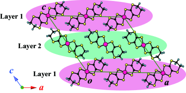
Figure 1: (Color online) Crystal structure of [Pd(dddt)₂] on the plane with the $\bm{a}$ and $\bm{c}$ axes. [25] The most conducting axis is given by $\bm{b}$ being perpendicular to the $\bm{a}$-$\bm{c}$ plane. There are four Pd(dddt)₂ molecules in the unit cell (the solid line), which consists of two layers shown by Layer 1 and Layer 2. Each molecule on an inversion center at Pd atom has HOMO and LUMO with the different parity.

2.1 Effective Hamiltonian

Figure 1 shows the crystal structure of the single-component molecular conductor [Pd(dddt)₂], where there are two layers, 1 and 2, that are crystallographically independent. The Dirac point is determined by the HOMO band of Layer 1 and the LUMO band of Layer 2. In the molecule, there is an inversion center at the Pd atom, where the HOMO and LUMO have different parities of ungerade and gerade symmetries. Since there are four molecules in the unit cell, there are eight energy bands, $E_{1}>E_{2}>E_{3}>\cdots>E_{8}$, where the upper (lower) four bands are mainly determined by the LUMO (HOMO). Under a high pressure of 8 GPa, the electronic state shows the Dirac point due to the reverse given by $E_{4}(\bm{k})$ for the HOMO and $E_{5}(\bm{k})$ for the LUMO close to the $\Gamma$ point. The tight-binding model shows that the Dirac points $\bm{k}_{0}$ with $E_{4}(\bm{k}_{0})=E_{5}(\bm{k}_{0})$ form a loop, i.e., a nodal line between the conduction and valence bands. [26] Such a line has been verified by first-principles DFT calculation. [31]

Figure 2(a) shows a nodal line obtained by the DFT calculation, [31] which is utilized in the present calculation. Although the shape of the line is slightly different from that of the tight-binding model, the condition of the Dirac point at the TRIM remains the same. [35] In the previous paper, [31] it was shown that the Dirac points in Fig. 2(a) can be obtained using a two-band model of the following effective Hamiltonian $H_{\rm eff}(\bm{k})$ in the form of a 2 $\times$ 2 matrix;

$${H_{\rm eff}(\bm{k})} = \begin{pmatrix}f_{0}(\bm{k})+f_{3}(\bm{k})&-if_{2}(\bm{k})\\ if_{2}(\bm{k})&f_{0}(\bm{k})-f_{3}(\bm{k})\end{pmatrix}\ .$$ (1)

The base is given by $|H(\bm{k})>$ and $|L(\bm{k})>$, the wave functions of $H^{0}(\bm{k})$ corresponding to HOMO and LUMO, i.e.,

$$H^{0}(\bm{k})|\alpha(\bm{k})>=E_{\alpha}(\bm{k})|\alpha(\bm{k})>\;$$ (2)

with $\alpha$ = H and L. $\bm{k}=(k_{x},k_{y},k_{z})$ denotes a 3D wave vector. $k_{x}$, $k_{y}$, and $k_{z}$ correspond to the reciprocal vector for $\bm{a}+\bm{c}$, $\bm{b}$, and $\bm{c}$, respectively. [25] Matrix elements $f_{0}(\bm{k})$, $f_{2}(\bm{k})$, and $f_{3}(\bm{k})$ in Eq. (1) are given by

$$f_{2}(\bm{k}) = i<{\rm H}(\bm{k})|H_{\rm int}|{\rm L}(\bm{k})>\;,$$ (3)

$$f_{3}(\bm{k}) = (E_{\rm H}(\bm{k})-E_{\rm L}(\bm{k}))/2\;,$$ (4)

$$f_{0}(\bm{k}) = (E_{\rm H}(\bm{k})+E_{\rm L}(\bm{k}))/2\;,$$ (5)

where $H_{\rm int}$ denotes the HOMO–LUMO (H–L) interaction. Although the off-diagonal element is treated by the perturbation, such an effective Hamiltonian is justified for the limiting case of $f_{2}(\bm{k})\rightarrow 0$, which is the present case of finding the Dirac point. The energy of Eq. (1) is calculated as $E_{\pm}=f_{0}\pm\sqrt{f_{2}^{2}+f_{3}^{2}}$, where $E_{+}(E_{-})=E_{c}(E_{v})$ corresponds to the energy of the conduction (valence) band. The Dirac point $\bm{k}_{\rm 0}$, which is given by $E_{+}=E_{-}$, is obtained from

$$f_{2}(\bm{k}_{\rm 0}) = 0\;,$$ (6a)

$$f_{3}(\bm{k}_{\rm 0}) = 0\;.$$ (6b)

Note that $f_{0}(\bm{k})$ and $f_{2}(\bm{k})$ are even functions of $\bm{k}$ because of time-reversal symmetry and $f_{2}(\bm{k})$ is an odd function of $\bm{k}$ because the HOMO and LUMO have different parities. Instead of calculating Eq. (2) directly, we utilize the numerical results of the DFT calculation as follows. The function $f_{2}(\bm{k})$ is estimated by projecting the nodal line on the $k_{x}$ - $k_{z}$ plane, while $f_{3}(\bm{k})$ is estimated by projecting the nodal line on the $k_{x}$ - $k_{y}$ plane. [31] Such a method is justified in the present because of the presence of the inversion symmetry at $k_{y}=0$.

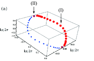
Figure 2: (Color online) (a) Nodal line in the 3D momentum space $(k_{x},k_{y},k_{z})$, which connects the Dirac point $\bm{k}_{\rm 0}[=(k_{\rm 0x},k_{\rm 0y},k_{\rm 0z})]$ calculated from first-principles calculation for the optimized structure at 8 GPa.[31] For example, Dirac points $\bm{k}_{\rm 0}[=(k_{\rm 0x},k_{\rm 0y},k_{\rm 0z})]$ which are scaled by $2\pi$ are given by (-0.1967, 0.000, 0.3924) (II), (0, 0.086, 0) (I), and (0.1967, 0.0, -0.3924) with decreasing $k_{z}$. The other points are taken from Ref. Tsumuraya2018_JPSJ. These Dirac points show a mirror symmetry in the plane of $k_{y}=0$, i.e., two points $(k_{\rm 0x},\pm k_{\rm 0y},k_{\rm 0z})$ are symmetric. The nodal line corresponding to the large symbols (i.e., $k_{y}\geq 0$ ) is examined in the present paper. (b) Energy $\delta E_{\rm D}(=E_{\rm D}-C_{0})$ in the unit of eV along the Dirac point as a function of $k_{z}(\equiv k_{z}/2\pi)$, where $C_{0}$ denotes $E_{\rm D}$ at $\bm{k}_{\rm 0}/2\pi$ = $(0,0.086,0)$ (I). For example, $\delta E_{\rm D}$ = 0 for (I), -0.00321 for (II), and -0.0064 (minimum) for (-0.143, 0.054, 0.238). The solid line was obtained by substituting $\bm{k}_{\rm 0}$ of Eqs. (6a) and (6b) into Eq. (9). The open squares show eigenvalues calculated using the first-principles band structure. The dotted line denotes the chemical potential $\mu$ at the Dirac points (-0.085, 0.075, 0.108) and (-0.191, 0.019, 0.372).

Here we discuss the linear dispersion in the present effective Hamiltonian of Eq. (1). Close to the Dirac point, we rewrite $f_{j}(\bm{k})$ as $f_{j}(\bm{k})\simeq f_{j}(\bm{k}_{\rm 0})+\bm{v}_{j}\cdot\delta\bm{k}$ ($j$ = 2, 3 and 0) with $\delta\bm{k}=\bm{k}-\bm{k}_{\rm 0}$, where $f_{2}(\bm{k}_{\rm 0})=f_{3}(\bm{k}_{\rm 0})=0$ and $f_{0}(\bm{k}_{\rm 0})\not=0$. Diagonalizing Eq. (1), the energy of the Dirac cone is obtained as $E_{\pm}(\bm{k})\simeq f_{0}(\bm{k}_{\rm 0})+\bm{v}_{0}\cdot\delta\bm{k}$ $\pm\sqrt{(\bm{v}_{2}\cdot\delta\bm{k})^{2}+(\bm{v}_{3}\cdot\delta\bm{k})^{2}}$. Thus, the energy difference corresponding to half the energy difference between the two bands is expressed as

$$\Delta_{\bm{k}} = [E_{+}(\bm{k})-E_{-}(\bm{k})]/2$$ (7)

$$=\sqrt{(\bm{v}_{2}\cdot\delta\bm{k})^{2}+(\bm{v}_{3}\cdot\delta\bm{k})^{2}}\;.$$

Note that the momenta $\delta{\bm{k}}$ forming this linear dispersion are within the $\bm{v}_{2}$-$\bm{v}_{3}$ plane. This plane is perpendicular to the tangent of the nodal line since the latter is parallel to $\bm{v}_{2}\times\bm{v}_{3}$.[30]

2.2 Calculation of matrix elements

In this subsection, we examine $f_{2}(\bm{k})$, $f_{3}(\bm{k})$, and $f_{0}(\bm{k})$ in terms of the power law of $\bm{k}$. Hereafter, we take the lattice constant as unity and scale $k_{x}$, $k_{y}$, and $k_{z}$ by 2$\pi$, i.e., $k_{\alpha}/2\pi\rightarrow k_{\alpha}$ for $\alpha=x,y$, and $z$. The unit of energy is taken as eV. First, to reproduce the nodal line in Fig. 2(a), [31] we determine

$$f_{2}(\bm{k}) \simeq C_{2}(k_{z}+k_{x}+40k_{x}^{3}-380k_{x}^{5})\;,$$ (8a)

$$f_{3}(\bm{k}) \simeq C_{3}((k_{x}/0.1967)^{2}+(k_{y}/0.086)^{2}$$ (8b)

$$+((k_{x}k_{y})^{2}/0.027^{2}-1)\;.$$

Compared with the previous case, [31] the present calculation was improved by adding arbitrary $C_{2}$ and $C_{3}$. Note that a non-coplanar nodal line is understood from the nonlinear terms in Eq. (8a). We have determined the coefficients in Eq. (8a) and (8b) except for $C_{2}$ and $C_{3}$ by comparing Eqs. (6a) and (6b) with Dirac points in Fig. 2(a). In fact, we used the two Dirac points (0,0.086,0) (I) and ( - 0.1967, 0, 0.3924) (II), and some other Dirac points in the intermediate region in Fig. 2(a). Coefficients $C_{2}$ and $C_{3}$, which also depend on the location on the nodal line, are determined using the velocities of Dirac points (I) and (II). Here, the velocity of the cone at the Dirac point $\bm{k}_{\rm 0}$ is obtained as $\bm{v}_{2}=\nabla_{\bm{k}_{\rm 0}}f_{2}$, $\bm{v}_{3}=\nabla_{\bm{k}_{\rm 0}}f_{3}$. [30] From the DFT calculation, the velocities at point (I) are $\bm{v}_{2}$ = (0.148, 0, 0.148) and $\bm{v}_{3}$ = (0, 1.25, 0), while the velocities at Dirac point (II) are $v_{x}\simeq 0.36$ and $v_{z}\simeq 0.09$. Furthermore, by interpolation between points (I) and (II), we obtain $C_{2}=0.148(1-0.39(k_{z}/0.392)^{2})$ and $C_{3}=0.053(1-0.53(k_{z}/0.392)^{2})$ for Eqs. (8a) and (8b).

Next, we examine $f_{0}({\bm{k}})$ assuming that it has the form

$$f_{0}(\bm{k}) \simeq b_{x}k_{x}^{2}+b_{y}k_{y}^{2}+b_{z}k_{z}^{2}$$ (9)

$$+bk_{x}^{2}k_{z}^{2}+d_{x}k_{y}^{2}k_{x}^{2}+d_{z}k_{y}^{2}k_{z}^{2}+C_{0}\;,$$

where $f_{0}(\bm{k}_{\rm 0})$ ( = $E_{\rm D}$) denotes the energy at Dirac point $\bm{k}_{\rm 0}$.

Figure 2(b) shows the energy of the Dirac points as a function of $k_{z}(\leftarrow k_{z}/2\pi)$, where the open squares denote the numerical results of the DFT calculation. Using these data to fit Eq. (9), we obtain $b_{x}=-0.88,b_{y}=-2.62,b_{z}=-0.069$, $b=3.7,d_{x}=-98$, and $d_{z}=32$. Note that terms with coefficients $b$, $d_{x}$, and $d_{z}$ are added in contrast to the previous case [31], since terms with only $b_{x}$, $b_{y}$ and $b_{z}$ are insufficient to reproduce the data in Fig. 2(b). The coefficients $b_{x}$, $b_{y}$, $b_{z}$, and $b$ in $f_{0}(\bm{k})$ are determined from $\delta E_{\rm D}(\equiv E_{\rm D}-C_{0})$ at Dirac point (II), and the tilting velocities $\bm{v}_{0}=(0,-0.45,0)$ and $\bm{v}_{0}=(0.12,0,0.06)$ at Dirac points (I) and (II), respectively. $C_{0}$ denotes $E_{\rm D}$ at Dirac point (I). Furthermore, coefficients $d_{x}$ and $d_{z}$ are determined from Dirac points (symbols) with $\delta E_{\rm D}$ = -0.0539 and -0.0642 close to the minimum in Fig. 2(b). The energy $E_{\rm D}$ (solid line) is calculated by substituting the Dirac point into Eq. (9), where $\bm{k}_{\rm 0}$ is obtained from Eqs. (6a) and (6b). It turns out that $E_{\rm D}$ (solid line) coincides reasonably well with that obtained from first-principles calculation (open squares).

The chemical potential $\mu$ (dotted line) is obtained from the condition of the half-filled band, which is shown later. It is found that the Fermi surface cuts the entire line eight times followed by the alternation of the hole and electron pockets, e.g., the hole pockets are obtained for (I) and (II).

From Eqs. (8a), (8b), and (9), the explicit form of $\bm{v}_{j}$ is given as

$$\bm{v}_{2} = \nabla_{\bm{k}_{\rm 0}}f_{2}\simeq C_{2}(1+120k_{\rm 0x}^{2}-1900k_{\rm 0x}^{4},0,1),$$ (10a)

$$\bm{v}_{3} = \nabla_{\bm{k}_{\rm 0}}f_{3}\simeq C_{3}(2k_{\rm 0x}/0.1967^{2}+2k_{\rm 0x}k_{\rm 0y}^{2}/0.027^{2},$$ (10b)

$$2k_{\rm 0y}/0.086^{2}+2k_{\rm 0x}^{2}k_{\rm 0y}/0.027^{2},0)\;,$$

$$\bm{v}_{0} = \nabla_{\bm{k}_{\rm 0}}f_{0}\simeq(2k_{\rm 0x}(b_{x}+bk_{\rm 0z}^{2}+d_{x}k_{\rm 0y}^{2}),$$ (10c)

$$2k_{\rm 0y}(b_{y}+d_{x}k_{\rm 0x}^{2}+d_{z}k_{\rm 0z}^{2}),$$

$$2k_{\rm 0z}(b_{z}+bk_{\rm 0x}^{2}+d_{z}k_{\rm 0y}^{2}))\;.$$

Although the derivatives of $C_{2}(\bm{k}_{\rm 0})$ and $C_{3}(\bm{k}_{\rm 0})$ with respect to $\bm{k}_{\rm 0}$ are finite, Eqs. (11a) and (10b) are still valid owing to $f_{2}(\bm{k}_{\rm 0})/C_{2}=0$ and $f_{3}(\bm{k}_{\rm 0})/C_{3}\ =0$.

Here, we mention the behaviors of the velocity of the Dirac cone in the region of $-0.3924\leq k_{z}\leq 0.3924$ and for $k_{y}\geq 0$, which corresponds to the line given by the large symbols in Fig. 2(a). An arbitrary $\bm{k}_{\rm 0}$ is calculated self-consistently from Eqs. (6a) and (6b) with Eqs. (8a) and (8b). Using these Dirac points, the velocities of the Dirac cone $\bm{v}_{2}$ and $\bm{v}_{3}$ are obtained from Eqs. (11a) and (10b). Velocities $\bm{v}_{2}(\bm{k}_{\rm 0})$ and $\bm{v}_{3}(\bm{k}_{\rm 0})$ as a function of $k_{z}$ show that $v_{2x}$, $v_{2z}$, and $v_{3y}$ are even but $v_{3x}$ is odd. The tilting velocities of the cone $\bm{v}_{0}(\bm{k}_{\rm 0})$ as a function of $k_{z}$ show that $v_{0y}$ and $v_{0x}$ are even but $v_{0z}$ is odd. These properties originate from $f_{3}(\bm{k})$ and $f_{0}(\bm{k})$ being even and $f_{2}(\bm{k})$ being odd with respect to $\bm{k}\rightarrow-\bm{k}$.

3 Properties of Dirac Cone

3.1 Unit vector along nodal line

Since $\bm{v}_{2}$ is not orthogonal to $\bm{v_{3}}$ except for $k_{0z}=0$, we calculate the principal axes to understand clearly the Dirac cone for an arbitrary Dirac point on the nodal line. First, we introduce a set of three orthogonal unit vectors, $\bm{e}_{1}$, $\bm{e}_{2}$, and $\bm{e}_{\perp}$. Quantities $\bm{e}_{2}$, $\bm{e}_{3}$, and $\bm{e}_{1}$ are unit vectors parallel to $\bm{v}_{2}$, $\bm{v}_{3}$, and $\bm{v}_{2}\times\bm{v}_{3}$, respectively. Since the direction of $\bm{e}_{1}$ is the tangent of the nodal line, the vectors of principal axes for the Dirac cone are located on the plane perpendicular to $\bm{e}_{1}$, i.e., on the $\bm{e}_{2}$-$\bm{e}_{3}$ plane. To consider the orthogonal basis on the $\bm{e}_{2}$-$\bm{e}_{3}$ plane, we introduce $\bm{e}_{\perp}(=\bm{e}_{1}\times\bm{e}_{2})$, which is orthogonal to both $\bm{e}_{1}$ and $\bm{e}_{2}$. These vectors expressed as

$$\bm{e}_{2}=\bm{v}_{2}/v_{2}=(v_{2x},0,v_{2z})/v_{2}\;,$$ (11a)

$$\bm{e}_{3}=\bm{v}_{3}/v_{3}=(v_{3x},v_{3y},0)/v_{3},$$ (11b)

$$\bm{e}_{1}=\bm{e}_{2}\times\bm{e}_{3}/|\bm{e}_{2}\times\bm{e}_{3}|\;,$$ (11c)

$$\bm{e}_{\perp}=\bm{e}_{1}\times\bm{e}_{2}\;,$$ (11d)

where $v_{2}=\sqrt{v_{2x}^{2}+v_{2z}^{2}}$ and $v_{3}=\sqrt{v_{3x}^{2}+v_{3y}^{2}}$. Figure 3(a) shows the components of $\bm{e}_{1}$ as a function of $k_{z}$; $e_{1y}$ is odd while $e_{1x}$ and $e_{1z}$ are even. With increasing $k_{z}$, $e_{1y}$ changes from 1 to -1, while the signs of $e_{1x}$ and $e_{1z}$ remain unchanged. Note that $\bm{e}_{1}$ with $k_{y}<0$ [small symbols in Fig. 2(a)] is obtained from $\bm{e}_{1}$ with $k_{y}>0$ by the replacement $(k_{\rm 0x},k_{\rm 0y},k_{\rm 0z})\rightarrow(-k_{\rm 0x},k_{\rm 0y},-k_{\rm 0z})$.

3.2 Principal axes and velocities

Next, we examine the principal axes of the linear dispersion $\Delta_{\bm{k}}$ of Eq. (7), which is expressed in terms of $\bm{e}_{2}$ and $\bm{e}_{\perp}$. Since $\bm{v}_{2}$ is not orthogonal to $\bm{v}_{3}$ except when $k_{z}=0$, we introduce $\phi$ as the angle between $\bm{v}_{2}$ and $\bm{v}_{3}$,

$$\cos\phi=(\bm{v}_{2}\cdot\bm{v}_{3})/(v_{2}v_{3})\;,$$ (12a)

where $$\phi-\pi/2 k_{z} |\cos\phi| |k_{z}| \Delta_{\bm{k}} \Delta({\bm{q}}) \bm{q}=\bm{k}-\bm{k}_{0}=q_{1}\bm{e}_{1}+q_{2}\bm{e}_{2}+q_{3}\bm{e}_{\perp} \cos\phi=\bm{e}_{2}\cdot\bm{e}_{3} \bm{v}_{2}=v_{2}\bm{e}_{2} \bm{v}_{3}=v_{3}\cos(\phi)\bm{e}_{2}+v_{3}\sin(\phi)\bm{e}_{\perp}$$ is an odd function of and increases monotonically with . When is expressed in terms of the principal axes, we note that , where , is written in terms of the principal axes. Noting that , , and , we obtain

$$\bm{v}_{2}\cdot\bm{q}=v_{2}q_{2}\;,$$ (12b)

$$\bm{v}_{3}\cdot\bm{q}=v_{3}q_{2}\cos\phi+v_{3}q_{3}\sin\phi\;.$$ (12c)

Thus, the explicit form of $\Delta(\bm{q})$ of Eq. (7) is written as

$$\Delta(\bm{q})^{2} = (\bm{v}_{2}\cdot\bm{q})^{2}+(\bm{v}_{3}\cdot\bm{q})^{2}$$ (13a)

$$=Aq_{2}^{2}+2Cq_{2}q_{3}+Bq_{3}^{2}\;,$$

$$A = v_{2}^{2}+(v_{3}\cos\phi)^{2}\;,$$ (13b)

$$B = v_{3}^{2}(\sin\phi)^{2}\;,$$ (13c)

$$C = v_{3}^{2}\sin\phi\cos\phi\;.$$ (13d)

The principal axes are obtained by rotation from the $q_{2}-q_{3}$ plane to the $q_{-}-q_{+}$ plane to eliminate the second term that is proportional to $q_{-}q_{+}$. The result is obtained as

$$\Delta(\bm{q})^{2} = V_{+}^{2}q_{+}^{2}+V_{-}^{2}q_{-}^{2}\;,$$ (14a)

$$V_{\pm}^{2} = \frac{1}{2}\left[A+B\pm\sqrt{(A-B)^{2}+4C^{2}}\right]\;,$$ (14b)

$$\tan(2\theta) = \frac{2C}{A-B}=\frac{v_{3}^{2}\sin 2\phi}{v_{2}^{2}+v_{3}^{2}\cos 2\phi}\;,$$ (14c)

where $q_{+}$ and $q_{-}$ are the rotated coordinates of principal axes given by

$$\bm{q}=q_{1}\bm{e}_{1}+q_{+}\bm{e}_{+}+q_{-}\bm{e}_{-}\;,$$ (15a)

$$\bm{e}_{-}=\cos\theta\bm{e}_{2}+\sin\theta\bm{e}_{\perp}\;,$$ (15b)

$$\bm{e}_{+}=-\sin\theta\bm{e}_{2}+\cos\theta\bm{e}_{\perp}\;.$$ (15c)

$\theta$ is the angle between $\bm{e}_{-}$ and $\bm{e}_{2}$ and is chosen to be $|\theta|\leq\pi/2$. $V_{+}$ and $V_{-}$ are the velocities of the principal axes. Note that $V_{+}>V_{-}$.

Figures 3(b) and 3(c) show the $k_{z}$ dependence of the unit vector, $\bm{e}_{\pm}$, for the respective principal axes. Figure 3(b) shows the component of $\bm{e}_{-}=(e_{-,x},e_{-,y},e_{-,z})$. As a function of $k_{z}$, $e_{-,x}$ and $e_{-,z}(>0)$ are even and $e_{-,y}$ is odd. $e_{-,z}$ takes a minimum and $\simeq 1$ for $k_{z}=\pm 0.3924$, while $e_{-,x}$ takes a maximum and decreases almost to zero for $|k_{z}|\simeq 0.3924$. With increasing $|k_{z}|$, $|e_{-,y}|$ increases linearly, followed by a sudden decrease to zero at $|k_{z}|\simeq 0.3924$. Figure 3(c) shows the $k_{z}$ dependence of the component for $\bm{e}_{+}=(e_{+,x},e_{+,y},e_{+,z})$. $e_{+,y}$ is an even function, where $e_{+,y}=1$ at $k_{z}=0$ and decreases to zero monotonically with $|k_{z}|$ increasing to 0.3924. $e_{+,x}$ and $e_{+z}$ are odd functions, and $e_{+,x}$ changes from $\simeq 1$ to $\simeq-1$. The variation of $e_{+,z}$ is much smaller than that of $e_{+,x}$. The rotation of $\bm{e}_{+}$ with $k_{z}$ increasing from $0$ to $0.3924$ is also reasonable compared with that of $\bm{e}_{-}$, because $\bm{e}_{+}\cdot\bm{e}_{-}=0$.

The cross section for $\Delta(\bm{k})=E_{0}$ is an ellipse with the radius of the minor (major) axis calculated as $a=E_{0}/V_{+}$ ($b=E_{0}/V_{-}$). Using $V_{+}$ and $V_{-}$, the area of the ellipse, $S$, for the gap $2E_{0}=E_{+}-E_{-}$ is given by $S(\bm{k}_{\rm 0})=\pi ab=\pi E_{0}^{2}/(V_{+}V_{-})$ $=\pi E_{0}^{2}/\sqrt{AB-C^{2}}$ $=\pi E_{0}^{2}/|\bm{v}_{2}(\bm{k}_{\rm 0})\times\bm{v}_{3}(\bm{k}_{\rm 0})|=\pi E_{0}^{2}/(v_{2}v_{3}|\sin\phi|)$. As a function of $|k_{z}|$, $S$ is almost constant but exhibits a rapid increase at large $|k_{z}|$.

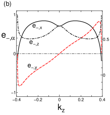
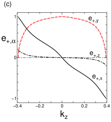
Figure 3: (Color online) (a) $k_{z}$ dependence of unit vector $\bm{e}_{1}$ [Eq. (11d)] parallel to the nodal line, where the components are given by $e_{1,x}$, $e_{1,y}$, and $e_{1,z}$. $e_{1y}$ is odd while $e_{1x}$ and $e_{1z}$ are even. $\bm{e}_{1}=(-1,0,1)/\sqrt{2}$ for $k_{z}=0$ and $\bm{e}_{1}=(0,\mp 1,0)$ for $k_{z}=\pm 0.3924$. (b) $k_{z}$ dependence of unit vector $\bm{e}_{-}$ [Eq. (15b)] for the principal axis of $V_{-}$, where the components are given by $e_{-,x}$, $e_{-,y}$, and $e_{-,z}$. (c) $k_{z}$ dependence of unit vector $\bm{e}_{+}$, [Eq. (15c)], for the principal axis of $V_{+}$, where the components are given by $e_{+,\alpha}$ ($\alpha=x,y,z)$. The vector $\bm{e}_{+}$ is also obtained from $\bm{e}_{+}=\bm{e}_{1}\times\bm{e}_{-}$ with $\bm{e}_{1}$ in (a).

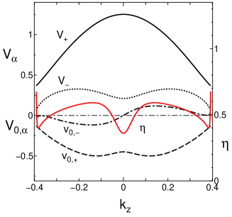
Figure 4: (Color online) Velocities $V_{+}$ and $V_{-}$, obtained from Eq. (14b). $v_{0\pm}$ [Eq. (16b)], denotes the tilting velocity for the corresponding axis. The quantity $\eta$ denotes a tilting parameter given by $\eta=((v_{0,-}/V_{-})^{2}+(v_{0,+}/V_{+})^{2})^{1/2}$, as shown in Eq. (18c).

Figure 4 shows the velocities $V_{\pm}$ obtained from Eq. (14b). The principal axes of the ellipsoid are obtained by a rotation of $\theta$ from the $q_{x}$-$q_{y}$ plane to the $q_{-}$-$q_{+}$ plane. The quantity $\theta$ is odd with respect to $k_{z}$ and becomes $\simeq\pm\pi/2$ for $k_{z}=\pm 0.3924$. The velocity $V_{+}$ decreases monotonically but $V_{-}$ takes a maximum with increasing $|k_{z}|$. Principal values $V_{\pm}$ ($V_{+}>V_{-}$) show a large anisotropy, where $V_{+}/V_{-}$ is maximum ($\simeq$ 6.0) at $k_{z}=0$ and minimum ($\simeq$ 2.3) at $|k_{z}|$ = 0.324.

3.3 Effect of tilting

We briefly mention the Dirac cone in the presence of the tilting velocity $\bm{v}_{0}$. In terms of $\bm{e}_{\pm}$, the tilting velocity is rewritten as

$$\bm{v}_{0} = (v_{0x},v_{0y},v_{0z}),$$ (16a)

$$= v_{0,1}\bm{e}_{1}+v_{0,-}\bm{e}_{-}+v_{0,+}\bm{e}_{+}\;,$$

$$v_{0,\pm} = \bm{v}_{0}\cdot\bm{e}_{\pm}\;,$$ (16b)

with $v_{0,1}=\bm{v}_{0}\cdot\bm{e}_{1}$. Figure 4 shows $v_{0,\pm}$, where $v_{0,-}$ ( $v_{0,+}$) is an odd (even) function with respect to $k_{z}$. By taking account of $\bm{v}_{0}\cdot\bm{q}$ with $\bm{q}=q_{-}\bm{e}_{-}+q_{+}\bm{e}_{+}$, the energy of the upper band $E_{+}(\bm{q})=E$ is written as

$$\sqrt{(V_{-}q_{-})^{2}+(V_{+}q_{+})^{2}}+v_{0.-}q_{-}+v_{0,+}q_{+}=E\;.$$ (17)

Defining $\tilde{q}_{\pm}=V_{\pm}q_{\pm}$, we examine the tilting on the plane of $\tilde{q}_{-}$ and $\tilde{q}_{+}$. Equation (17) is rewritten as

$$\sqrt{\tilde{q}_{-}^{2}+\tilde{q}_{+}^{2}}+\vec{\delta}\cdot(\tilde{q}_{-}\bm{e}_{-}+\tilde{q}_{+}\bm{e}+)=E\;,$$ (18c)

$$\vec{\delta}=(v_{0,-}/V_{-})\bm{e}_{-}+(v_{0.+}/V_{+})\bm{e}_{+}\;,$$

$$\eta=|\vec{\delta}|=\sqrt{(v_{0,-}/V_{-})^{2}+(v_{0,+}/V_{+})^{2}}\;.$$

The quantity $\eta$ denotes a tilting parameter and its $k_{z}$ dependence is shown in Fig. 4. The Dirac cone is tilted but not overtilted because $\eta<1$. Defining $\theta^{\prime}$ by $\bm{e}_{-}\sin\theta^{\prime}-\bm{e}_{+}\cos\theta^{\prime}=\vec{\delta}/|\vec{\delta}|$, Eq. (18c) is rewritten as

$$(1-\eta^{2})Q_{-}^{2}+(1-\eta^{2})^{2}\left(Q_{+}-\frac{E\eta}{1-\eta^{2}}\right)^{2}=E^{2}\;,\;\;\;$$

where

$$\tilde{q}_{-}\bm{e}_{-}+\tilde{q}_{+}\bm{e}_{+}=Q_{-}\bm{e}_{\delta 2}+Q_{+}\bm{e}_{\delta 1}\;,$$ (19b)

$$\bm{e}_{\delta 2}=\cos\theta^{\prime}\bm{e}_{-}+\sin\theta^{\prime}\bm{e}_{+}\;,$$ (19c)

$$\bm{e}_{\delta 1}=-\sin\theta^{\prime}\bm{e}_{-}+\cos\theta^{\prime}\bm{e}_{+}\;,$$ (19d)

$$\sin\theta^{\prime}=\frac{(v_{0,-}/V_{-})}{\eta}\;.$$ (19e)

Equation (19) shows an ellipsoid with radius $E(1-\eta^{2})^{-1}$ [$E(1-\eta^{2})^{-1/2}$] for $Q_{+}(Q_{-})$. The center is located at $[E\eta/(1-\eta^{2})](-\sin\theta^{\prime},\cos\theta^{\prime})$ on the plane of $\tilde{q}_{-}$ and $\tilde{q}_{+}$. The phase $\theta^{\prime}$ is the angle between $\bm{e}_{\delta,2}$ and $\bm{e}_{-}$, where $\bm{e}_{\delta,1}$ and $\bm{e}_{\delta,2}$ are orthogonal to each since due to $\bm{e}_{+}\cdot\bm{e}_{-}=0$. For $k_{z}=0$, the principal axis is given by $\bm{e}_{+}=\bm{e}_{\delta 1}$, i.e., $\tilde{q}_{+}=Q_{+}$ with $\theta^{\prime}=0$ owing to $v_{0,-}=0$. Thus, the rotation angle of the axes of the ellipsoid is obtained as $\theta^{\prime}$, i.e., $Q_{-}=\tilde{q}_{-}\cos\theta^{\prime}+\tilde{q}_{+}\sin\theta^{\prime}$ and $Q_{+}=-\tilde{q}_{-}\sin\theta^{\prime}+\tilde{q}_{+}\cos\theta^{\prime}$ from Eqs. (19b), (19c), and (19d). Note that it is straightforward to calculate the anisotropic conductivity by projecting the electric field on the axes of $\bm{e}_{\delta,1}$ and $\bm{e}_{\delta,2}$. [36]

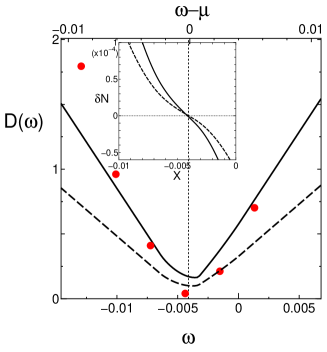
Figure 5: (Color online) Density of states (DOS) as a function of $\omega$ (solid line), which is given by Eq. (21). The origin is taken at $E_{d}$ of Dirac point (1). The dashed line denotes the DOS without tilting. The inset denotes the corresponding $\delta N$, which is given by Eq. (20). The vertical dotted line denotes the location of the chemical potential. The closed circles denote DOS values obtained by the first-principles DFT calculation.

4 Electronic States and Response to Magnetic Field

In this section, the present effective Hamiltonian is applied to calculate the density of states and orbital magnetic susceptibility.

4.1 Density of states

To calculate the number of states, we note that the area of the ellipse of the Dirac cone with $\mu=E_{0}$ is given by $S(\bm{k}_{\rm 0})=\pi E_{0}^{2}/(V_{+}V_{-})$. Here $V_{+}V_{-}$ turns out to be $v_{2}v_{3}|\sin\phi|$ from Eqs. (13b), (13c), (13d), (14a), and (14b). Furthermore, this area is modified as $S/(1-\eta^{2})^{3/2}$ in the presence of tilting, as can be seen from Eq. (19). Taking the origin of the number at the respective Dirac point, the deviation of the total number of states from that of a half-filled band is calculated as

$$\delta N(X) = \int_{\overline{C}}{\rm d}\bm{s}\cdot\bm{e}_{1}\;\;\;(\delta E_{D}(\bm{k}_{0})-X)^{2}$$ (20)

$$\times\frac{2\pi\;{\rm sgn}(\delta E_{D}(\bm{k}_{0})-X)}{v_{2}v_{3}|\sin(\phi)|(1-\eta^{2})^{3/2}}\;,$$

where $X$ and $\delta E_{D}(\bm{k}_{0})$ are measured from the energy of the Dirac point (I), i.e., $E_{D}(\bm{k})$ at $\bm{k}=(0,0.086,0)$. The quantity $X$ is introduced as a chemical potential, which gives the variation of $\delta N(X)$. Here, $\int_{\overline{C}}$ represents the integral [corresponding to large symbols in Fig. 2(a)], and the integral is performed using $\int{\rm d}\bm{s}\cdot\bm{e}_{1}=\int{\rm d}z/{\rm e}_{1z}$. From $\delta N(X)$, the DOS is given by

$$D(\omega) = -\frac{\partial(\delta N)}{\partial X}|_{X=\omega}\;.$$ (21)

In Fig. 5, the solid lines show $D(\omega)$ and $\delta N(X)$ (in the inset) as a function of $\omega$ (or $X$). Note that $X$ at which $\delta N(X)=0$ holds corresponds to the chemical potential $\mu$. This gives $\mu=-0.0041$, as can be seen in Fig. 5. The dashed line denotes the DOS without tilting, i.e., $\eta=0$, which is lower than the solid line, because the tilting increases the area of the ellipsoid, $S$, with fixed energy $E_{0}$. Within the numerical accuracy, one finds the relation (see the top $x$-axis in Fig. 5)

$$D(\omega-\mu)\propto|\mu-\omega|\;,$$ (22)

for $0.005<|\omega-\mu|$, while there is a slight deviation for $|\omega-\mu|<0.005$. This comes from the nonmonotonic variation of $E_{D}$ with respect to $k_{z}$, as seen in Fig. 2(b).

Next, we compare the above results with those in the DFT calculation. To obtain DOS using the first-principles DFT method, we need a more elaborate numerical calculation than that described in Sect. 2. For this purpose, $\bf{k}$-point meshes are taken as 16 $\times$ 32 $\times$ 16 for the DFT-optimized structure under the pressure of 8 GPa, [25, 31] where Kohn–Sham equations are self-consistently solved in a scalar-relativistic fashion by the all-electron full-potential linearized augmented plane wave (FLAPW) method[37, 38, 39] within an exchange-correlation functional of a generalized gradient approximation (GGA)[40]. The obtained DOS values are shown in Fig. 5 by the closed circles. The finite DOS for small $\omega$ suggests a metallic behavior. This is qualitatively consistent with the experimental results [28] and also with the solid line in Fig. 5, while the behavior close to the minimum shows a deviation from the solid line. Thus, the present calculation in terms of the effective model may provide reasonable results for a nodal line semimetal.

4.2 Some properties of non-coplanar nodal loop

In this subsection, we clarify several properties of the nodal line (loop). First, we define the average for some quantity $F$ along the nodal line by

$$<F>=\frac{\int_{\overline{C}}{\rm d}\bm{s}\cdot\bm{e}_{1}\;F}{\int_{\overline{C}}{\rm d}\bm{s}\cdot\bm{e}_{1}}\;.$$ (23)

In the present nodal line, a length of the line is obtained as $L=2\int_{\overline{C}}{\rm d}\bm{s}\cdot\bm{e}_{1}$ = 1.856, which is smaller than 4, being the length of the square of the Brillouin zone. This can be verified by noting that the present nodal line is almost an ellipse with major axis $a\simeq 0.44$ and minor axis $b\simeq 0.086$. The ellipse length $\tilde{L}$ is given by $\tilde{L}=4aE(k)$ with $k^{2}=1-(b/a)^{2}$, $E(k)$ being the complete elliptic integral of the second kind defined by $E(k)=\int^{\pi/2}_{0}[1-k^{2}\sin^{2}x]^{1/2}dx$. Since $E(k)\simeq 1.05$ with $k^{2}=0.96$ for the present case, we obtain $\tilde{L}=1.85\simeq L$, which well reproduces the above numerical result. Furthermore, the area of the nodal line (ellipse) is estimated as $\pi ab=\pi\tilde{L}^{2}(1-k^{2})^{1/2}/(16E(k)^{2})\simeq 0.118$, which is much smaller than 1, corresponding to the area of the first Brillouin zone.

Figure 6: (Color online) Orbital magnetic susceptibility $\chi_{N}$ under magnetic field $\bm{B}$ $(=B\bm{e}_{B})$ applied in the plane of the nodal line and given by Eq. (26). The phase $\phi$ is the rotation angle around a normal vector $\bm{e}_{np}[=(\sin\theta_{0},0,\cos\theta_{0})]$ perpendicular to the plane of the nodal line, where $\bm{e}_{B}=(-\cos\theta_{0},0,\sin\theta_{0})$ for $\phi=0$. Line (1) corresponds to a half-filled band and line (2) denotes a case of hole doping, where the chemical potential is given by $\delta\mu$ = 0 (1) and -0.003 (2). $\delta\mu=\mu-\mu_{0}$ and $\mu_{0}$ = -0.0041. The dashed line denotes $R$ defined by $R=\chi_{N}/<(\bm{e}_{B}\cdot\bm{e}_{1})^{2}>$, which is almost constant except in the region close to the minimum (at $\phi/\pi=0.5$). In the inset, $E_{L}$ is shown as a function of $\phi/\pi$ for a magnetic field perpendicular to the normal vector $\bm{e}_{np}$.

Next, to examine the plane of the nodal line, we calculate a unit vector $\bm{e}_{np}$ perpendicular to the plane. Since the present nodal line is non-coplanar, the condition $\bm{e}_{np}\cdot\bm{e}_{1}=0$ is not always satisfied on the line. Therefore, we determine $\bm{e}_{np}$ to give the minimum $<|\bm{e}_{np}\cdot\bm{e}_{1}|>$, where $\bm{e}_{1}$ is given by Fig. 3(a). Because of the mirror symmetry at $k_{y}=0$, we calculate $\bm{e}_{np}$ in the form of $\bm{e}_{np}=(\sin\theta,0,\cos\theta)$, where $\theta$ denotes the angle between $\bm{e}_{z}$ and $\bm{e}_{np}$. The minimum $<|\bm{e}_{np}\cdot\bm{e}_{1}|>$ is obtained at $\theta=\theta_{0}\simeq 0.36\pi$, where $<|\bm{e}_{np}\cdot\bm{e}_{1}|>\simeq 0.029$. This means that the deviation of the nodal line from te plane is moderately small.

4.3 Orbital magnetic susceptibility

As one of the characteristic physical quantities, we calculate the orbital susceptibility for the nodal line semimetal. It is well known that the two-dimensional massless Dirac electrons (or electrons in graphene) give a delta-function-like orbital magnetic susceptibility, [41, 42, 43]

$$\chi_{\rm GR}=-\frac{e^{2}v^{2}}{3\pi^{2}\Gamma_{0}}\frac{1}{1+X_{0}^{2}},$$ (24)

where $v$ is the velocity of the Dirac cone, $X_{0}=\mu/\Gamma_{0}$, and the relaxation rate $\Gamma_{0}$ has been introduced phenomenologically. Note that in the limit of $\Gamma_{0}\rightarrow 0$, $1/\Gamma_{0}(1+X_{0}^{2})$ becomes $\pi\delta(\mu)$. The effect of tilting on the magnetic susceptibility was studied previously.[44, 45] Here we use

$$\chi_{\rm tilting}=-\frac{e^{2}v^{2}}{3\pi^{2}\Gamma_{0}}\frac{1}{1+X_{0}^{2}}(1-\eta^{2})^{3/2}.$$ (25)

In this study, we estimate the orbital magnetic susceptibility $\chi$ for the present nodal line, assuming that $\chi$ is given by the sum of $\chi_{\rm tilting}$ over the nodal line. To study the angle dependence of $\chi$, the direction of the magnetic field is chosen to be within the nodal plane. For this purpose, the unit vector of the magnetic field, $\bm{e}_{B}=\bm{B}/B$, is taken as

$$\bm{e}_{B}=(-\cos\phi\cos\theta_{0},\sin\phi,\cos\phi\sin\theta_{0})\;,$$ (26)

so that $\bm{B}$ is always perpendicular to $\bm{e}_{np}=(\sin\theta_{0},0,\cos\theta_{0})$. The phase $\phi$ represents the angle of $\bm{B}$ and is chosen such that $\bm{e}_{B}=(-\cos\theta_{0},0,\sin\theta_{0})$ when $\phi=0$. Therefore, the phase $\phi=0$ corresponds to the case where $\bm{B}$ is parallel to the tangential direction at Dirac point (I). In the same way, $\phi=\pi/2$ corresponds to the case where $\bm{B}$ is tangential at Dirac point (II).

Since the principal axes for the Dirac cone are located in the $\bm{e}_{2}$-$\bm{e}_{3}$ plane, the effective magnetic field is considered to be $(\bm{e}_{B}\cdot\bm{e}_{1})B$. Taking account of the variation of velocities and $\delta E_{\rm D}$ along the nodal line, $\chi$ is written as

$$\chi=-\frac{e^{2}<V_{+}V_{-}>L}{3\pi^{2}\Gamma_{0}}\chi_{N}\;,$$ (27a)

$$\chi_{N}=\left<(\bm{e}_{B}\cdot\bm{e}_{1})^{2}\frac{V_{+}V_{-}}{<V_{+}V_{-}>}\frac{1}{1+\tilde{X}^{2}}(1-\eta^{2})^{3/2}\right>\;,$$

(27b)

where $$\tilde{X}=(\mu-\delta E_{D})/\Gamma_{0} \Gamma_{0}=0.001 V_{\pm},\eta \tilde{X} \chi_{N} \phi \chi_{N} \chi_{N}\simeq \phi/\pi \chi_{N}\simeq \phi/\pi \chi \bm{B} \bm{e}_{1} \chi_{N} \phi/\pi$$ with . Quantities , and vary along the 3D nodal line [Fig. 2(a)]. Figure 6 shows [line (1)] as a function of , where is maximum, 0.0165, at = 0 and 1, and minimum, 0.0003, at = 0.5. This means that the maximum (minimum) occurs when is parallel to at Dirac point (I) (Dirac point (II)). The reason why is minimum at = 0.5 is that the Dirac cone near Dirac point (II) is fairly distorted, as seen from Figs. 3(b), 3(c), and 4. The experimental observation of such an extremum will be useful in finding the direction of the principal axis of the nodal plane.

We examine $\chi_{N}$ using a quantity $R$ given by

$$R=\frac{\chi_{N}}{<(\bm{e}_{B}\cdot\bm{e}_{1})^{2}>}\;,$$ (27c)

which is shown as a function of $\phi$ in Fig. 6. The quantity $R$ gives an estimation of the average of orbital magnetic susceptibility along the nodal line without considering the weight, $(\bm{e}_{B}\cdot\bm{e}_{1})^{2}$. We obtain $R\simeq 0.2477$ at $\phi/\pi$ = 0 and $R\simeq 0.2293$ at $\phi/\pi$ =0.5. Since the variation of $R$ is small compared with that of $\chi_{N}$, the $\phi$ dependence of $\chi_{N}$ is essentially determined by $(\bm{e}_{B}\cdot\bm{e}_{1})^{2}$, i.e., the geometric property of the nodal line. The average of the respective quantities in Eq. (27b) is estimated as $<V_{+}V_{-}>$ = 0.2462, $\sqrt{<\eta^{2}>}$ = 0.528, $<1/(1+\tilde{X}^{2})>$ = 0.364, and $<(\bm{e}_{B}\cdot\bm{e}_{1})^{2}>$ = 0.0665 (for $\phi/\pi$ = 0), and $<(1-\eta^{2})^{3/2}>$ = 0.614. Furthermore, we note that $(1-<\eta^{2}>)^{3/2}\simeq 0.612$. Using the average quantity, we obtain $<1/(1+\tilde{X}^{2})><(1-\eta^{2})^{3/2}>\simeq$ 0.223, which is slightly smaller than $R$ in Fig. 6. Such an enhancement of $R$ compared with the product of the average quantities comes from a combined effect of $(\bm{e}_{B}\cdot\bm{e}_{1})^{2}$, $V_{+}V_{-}$, $1/(1+\tilde{X}^{2})$, and $(1-\eta^{2})^{3/2}$.

Here, we briefly mention the effect of carrier doping, which is given by the variation of chemical potential, i.e., $\delta\mu(=\mu-\mu_{0})$ with $\mu_{0}$= - 0.0041. In Fig. 6, $\chi_{N}$ for hole doping is shown by line (2) with $\delta\mu$ = -0.003, which is smaller than that of line (1). Note that,the $\phi$-dependence of $\chi_{N}$ does not change qualitatively. We find that, with decreasing $\delta\mu$, $\chi_{N}$ first becomes maximum at $\delta\mu$ = -0.0018 and decreases rapidly, whereas $\chi_{N}$ decreases monotonically for increasing $\delta\mu(>0)$. Such asymmetry comes from that of the DOS (Fig. 5) and the variation in the energy $\delta E_{\rm D}$ on the nodal line in Fig. 2(a).

Finally, we discuss the average Landau level of the nodal line for a magnetic field $\bm{B}=B\bm{e}_{B}$ in the nodal plane. The $N$th Landau level is given by $E_{\pm N}=\pm\sqrt{2Ne\hbar B(1-\eta^{2})^{3/2}v^{2}}$ [46]. When we take the average over the nodal line, we obtain $E_{\pm N}=\pm\sqrt{2Ne\hbar B}<\sqrt{V_{+}V_{-}}>E_{L}+E_{0}$, where

$$E_{L}=\frac{<\sqrt{V_{+}V_{-}}(1-\eta^{2})^{3/4}\sqrt{|\bm{e}_{B}\cdot\bm{e}_{1}|}>}{<\sqrt{V_{+}V_{-}}>}\;.$$ (28)

The quantity $E_{0}$ is the average energy of the zeroth Landau level measured from the chemical potential, which is given by $<\delta E_{D}(\bm{k}_{0})-\mu>\simeq-0.0002$. The $\eta$-dependence of Eq. (28) has a common feature with that of Eq. (25), suggesting that the effect of the magnetic field on the Landau orbit is reduced by a factor of $(1-\eta^{2})^{3/2}$ [47]. In the inset of Fig. 6, $E_{L}$ is shown as a function of $\phi$ for a magnetic field perpendicular to $\bm{e}_{np}=(\sin\theta_{0},0,\cos\theta_{0})$. Note that $E_{L}$ in the plane perpendicular to $(\sin\theta,0,\cos\theta)$ is maximum at $\theta=\theta_{0}$. The behavior in the inset is similar to that of $\chi_{N}$ but differs at around $\phi/\pi=1/2$. $|E_{\pm 1}|$ will be identified when $|E_{\pm 1}|$ is larger than the variation of $\delta E_{D}$. For a two-dimensional organic conductor,[48] it has been claimed that the peak of the temperature dependence of interlayer longitudinal magnetoresistance is associated with the energy separation between the $N=0$ and $N=\pm 1$ Landau levels. Therefore, if the $\phi$-dependence of $|E_{\pm 1}|$ is estimated from such a magnetoresistance experiment, we can find the direction of the principal axis of the nodal line.

5 Summary

We examined an effective Hamiltonian of a two-band model, which describes the Dirac cone close to the nodal line of a molecular conductor [Pd(dddt)₂] with a half-filled band. The energy with a dispersion perpendicular to the nodal line was evaluated using the Dirac points obtained by the DFT calculation. The energy difference between the conduction and valence bands was calculated to obtain the principal axes and corresponding velocities, $V_{+}$ and $V_{-}$, which rotate along the nodal line. Furthermore, the effect of tilting on the Dirac cone was examined, where the mutual relationship between the principal axis and the tilting direction was clarified. The Dirac cone obtained by varying the nodal line gave reasonable energies, since the density of states showing the characteristics of the nodal line semimetal was i compatible with that obtained by the DFT calculation. The determination of the tilting axis of the respective Dirac cone in terms of the original momentum space $\bm{k}$ is useful for calculaing an response to the external field with arbitrary direction. As an example, we demonstrated the angular dependence of orbital magnetic susceptibility $\chi_{N}$, where the magnetic field was applied in the plane of the nodal line. Finally, we noted that the present method of deriving the effective Hamiltonian for the Dirac cone could be applied to other systems of a nodal line with an inversion symmetry.

- [1] S. Murakami, New J. Phys. 9, 356 (2007).
- [2] A. A. Burkov, D. Hook, and L. Balents, Phys. Rev. B 84, 235126 (2011).
- [3] C. Fang, H. Weng, X. Dai, and Z. Fang, Chin. Phys. B 25, 117106 (2016).
- [4] M. Hirayama, R. Okugawa, and S. Murakami, J. Phys. Soc. Jpn. 87, 041002 (2018).
- [5] A. Bernevig, H. Weng, Z. Fang, and X. Dai, J. Phys. Soc. Jpn. 87, 041001 (2018).
- [6] C. Fang, Y. Chen, H.-Y. Kee, and L. Fu, Phys. Rev. B 92, 081201 (2015).
- [7] M. Hirayama, R. Okugawa, T. Miyake, and S. Murakami, Nat. Commun. 8, 14022 (2017).
- [8] H. Huang, J. Liu, D. Vanderbilt, and W. Duan, Phys. Rev. B 93, 201114(R) (2016).
- [9] A. Yamakage, Y. Yamakawa, Y. Tanaka, and Y. Okamoto, J. Phys. Soc. Jpn. 85, 013708 (2016).
- [10] Y. Quan, Z. P. Yin, and W. E. Pickett, Phys. Rev. Lett. 118, 176402 (2017).
- [11] Y. Kim, B. J. Wieder, C. L. Kane, and A. M. Rappe, Phys. Rev. Lett. 115, 036806 (2015).
- [12] R. Yu, H. Weng, Z. Fang, X. Dai, and X. Hu, Phys. Rev. Lett. 115, 036807 (2015).
- [13] L. S. Xie, L. M. Schoop, E. M. Seibel, Q. D. Gibson, W. Xie, and R. J. Cava, APL Mater. 3, 083602 (2015).
- [14] K. Mullen, B. Uchoa, and D. T. Glatzhofer, Phys. Rev. Lett. 115, 026403 (2015).
- [15] I. Takeishi and H. Matsuura, J. Phys. Soc. Jpn. 87, 073702 (2018).
- [16] L. M. Schoop, M. N. Ali, C. Strasser, A. Topp, A. Varykhalov, D. Marchenko, V. Duppel, S. S. Parkin, B. V. Lotsch, and C. R. Ast, Nat. Commun. 7, 11696 (2016).
- [17] Y. Okamoto, T. Inohara, A. Yamakage, Y. Yamakawa, and K. Takenaka, J. Phys. Soc. Jpn. 85, 123701 (2016).
- [18] X. Wang, X.-M. Ma, E. Emmanouilidou, B. Shen, C.-H. Hsu, C.-S. Zhou, Y. Zuo, R.-R. Song, S.-Y. Xu, G. Wang, L. Huang, N. Ni, and C. Liu, Phys. Rev. B 96, 161112 (2017).
- [19] D. Takane, K. Nakayama, S. Souma, T. Wada, Y. Okamoto, K. Takenaka, Y. Yamakawa, A. Yamakage, T. Mitsuhashi, K. Horiba, H. Kumigashira, T. Takahashi, and T. Sato, npj Quantum Mater. 3, 1 (2018).
- [20] S.-Y. Yang, H. Yang, E. Derunova, S. S. P. Parkin, B. Yan, and M. N. Ali, Adv. Phys. X 3, 1414631 (2018).
- [21] C. Herring, Phys. Rev. 52, 365 (1937).
- [22] L. Fu and C. L. Kane, Phys. Rev. B 76, 045302 (2007).
- [23] L. Fu, C. L. Kane, and E. J. Mele, Phys. Rev. Lett. 98, 106803 (2007).
- [24] Z. Song, T. Zhang, and C. Fang, Phys. Rev. X 8, 031069 (2018).
- [25] R. Kato, H. Cui, T. Tsumuraya, T. Miyazaki, and Y. Suzumura, J. Am. Chem. Soc. 139, 1770 (2017).
- [26] R. Kato and Y. Suzumura, J. Phys. Soc. Jpn. 86, 064705 (2017).
- [27] Y. Suzumura, J. Phys. Soc. Jpn. 86, 124710 (2017).
- [28] Y. Suzumura, H. Cui, and R. Kato, J. Phys. Soc. Jpn. 87, 084702 (2018).
- [29] Z. Liu, H. Wang, Z. F. Wang, J. Yang, and F. Liu, Phys. Rev. B 97, 155138 (2018).
- [30] Y. Suzumura and A. Yamakage, J. Phys. Soc. Jpn. 87, 093704 (2018).
- [31] T. Tsumuraya, R. Kato, and Y. Suzumura, J. Phys. Soc. Jpn. 87, 113701 (2018).
- [32] S. Katayama, A. Kobayashi, and Y. Suzumura, J. Phys. Soc. Jpn. 75, 054705 (2006).
- [33] K. Kajita, Y. Nishio, N. Tajima, Y. Suzumura, and A. Kobayashi, J. Phys. Soc. Jpn. 83, 072002 (2014).
- [34] F. Piéchon and Y. Suzumura, J. Phys. Soc. Jpn. 82, 033703 (2013).
- [35] T. Tsumuraya, H. Sawahata, F. Ishii, H. Kino, R. Kato, and T. Miyazaki, Am. Phys. Soc. Bull., R14.00012 (2018).
- [36] Y. Suzumura, I. Proskurin, and M. Ogata, J. Phys. Soc. Jpn. 83, 023701 (2014).
- [37] E. Wimmer, H. Krakauer, M. Weinert, and A. J. Freeman, Phys. Rev. B 24, 864 (1981).
- [38] D. D. Koellng and G. O. Arbman, J. Phys. F: Met. Phys. 5, 2041 (1975).
- [39] M. Weinert, J. Math. Phys. 22, 2433 (1981).
- [40] J. P. Perdew, K. Burke, and M. Ernzerhof, Phys. Rev. Lett. 77, 3865 (1996).
- [41] J. M. McClure, Phys. Rev. 119, 606 (1960).
- [42] H. Fukuyama, Prog. Theor. Phys. 45, 704 (1971).
- [43] H. Fukuyama, J. Phys. Soc. Jpn. 76, 043711 (2007).
- [44] A. Kobayashi, Y. Suzumura, and H. Fukuyama, J. Phys. Soc. Jpn. 77, 064718 (2008).
- [45] The last factor of Eq. (25) is different from that obtained in Ref. \citenKobayashi2008. Its justification will be disccussed elsewhere. However, such a difference has no qualitative effect on the angular dependence of magnetic susceptibility in the present workr.
- [46] T. Morinari, T. Himura, and T. Tohyama, J. Phys. Soc. Jpn. 78, 023704 (2009).
- [47] Similar reduction was disccussed in the case of the Landau levels made by an electric field [V. Lukose, R. Shankar, and G. Baskaran, Phys. Rev. Lett. 98, 116802 (2007)].
- [48] S. Sugawara, M. Tamura, N. Tajima, R. Kato, M. Sato, Y. Nishio, and K. Kajita, J. Phys. Soc. Jpn. 79, 113704 (2010).