Symbol Message Passing Decoding of Nonbinary Low-Density Parity-Check Codes

Abstract

We present a novel decoding algorithm for $q$-ary low-density parity-check codes, termed symbol message passing. The proposed algorithm can be seen as a generalization of Gallager B and the binary message passing algorithm by Lechner et al. to $q$-ary codes. We derive density evolution equations for the $q$-ary symmetric channel, compute thresholds for a number of regular low-density parity-check code ensembles, and verify those by Monte Carlo simulations of long channel codes. The proposed algorithm shows performance advantages with respect to an algorithm of comparable complexity from the literature.

I Introduction

There is a large body of literature considering message passing algorithms for binary low-density parity-check (LDPC) codes. In his seminal work [1], Gallager proposed two different message passing algorithms for LDPC codes, nowadays known as Gallager A and B, which exchange binary messages between check nodes and variable nodes. In [2], algorithm E was proposed, where messages take values in a ternary alphabet. A powerful algorithm, referred to as binary message passing (BMP) was introduced in [3]. Although the exchanged messages are binary, the algorithm is able to exploit soft information from the channel at the VNs. An extension of BMP to ternary message alphabets was studied in [4]. A finite alphabet message iterative decoder for the binary symmetric channel (BSC) was presented in [5].

Various works in the literature study the extension of binary LDPC codes to larger fields, including the original work by Gallager [1]. Nonbinary LDPC codes constructed over finite fields for binary-input Gaussian channels were investigated in [6]. Different simplified message passing algorithms were studied in [7, 8]. Regarding $q$-ary symmetric channels, a majority-logic-like decoding algorithm was introduced in [9], while verification based decoding algorithms were studied in [10, 11, 12, 13]. Both algorithms target large field orders. In [14] a list message passing decoding algorithm for $q$-ary LDPC codes over the $q$-SC was proposed, which is practical when the list size is small. For list size 1, the exchanged messages take values in a $(q+1)$-ary message alphabet, composed of the elements of $\mathbb{F}_{q}$ and an additional erasure message. In [15] a decoding algorithm for $q$-ary LDPC codes was presented, for which the CN and VN operations are implemented by means of look up tables. It makes use of the information bottleneck method and is practical for small $q$.

This paper targets $q$-ary LDPC codes for which we propose a low-complexity decoding algorithm, termed symbol message passing (SMP). The proposed algorithm can be seen as an extension of BMP to $q$-ary codes and $q$-ary message alphabets. Similarly to BMP, it can exploit soft information from the channel at the VNs. Over the $q$-SC, SMP becomes a natural generalization of Gallager B [1]. We develop a density evolution (DE) analysis for SMP over the $q$-SC. For large $q$, the evaluation of DE becomes infeasible, due to the increasing complexity. To tackle this, we derive tight upper and lower bounds on the iterative decoding thresholds, which can be efficiently evaluated even for very large $q$. Simulation results are compared with the decoding thresholds obtained via DE. Both the analysis and the simulations are provided for the case of regular LDPC code ensembles for ease of exposition. However, the extension to irregular ensembles is straightforward. For the considered ensembles, the derived thresholds are superior to the ones obtained in [14] with list size $1$.

The proposed algorithm is of interest, among others, for applications with high decoding throughput and low decoding complexity requirements, such as optical communications. Another application area is code-based post-quantum cryptography, for which binary regular LDPC codes are considered in the literature [16]. Nonbinary codes can render cryptanalysis more difficult, but there is the need for simple decoders.

II Preliminaries

In this work, we consider regular $(\mathsf{d_{v}},\mathsf{d_{c}})$ LDPC codes constructed over a finite field of order $q$, $\mathbb{F}_{q}$. The code’s bipartite graph comprises $n$ VNs $\mathtt{v}_{j}$, $j=\{1,2,\ldots,n\}$ of degree $\mathsf{d_{v}}$ and $m$ CNs $\mathtt{c}_{i}$, $i=\{1,2,\ldots,m\}$ of degree $\mathsf{d_{c}}$. The design rate is $R=1-m/n=1-\mathsf{d_{v}}/\mathsf{d_{c}}$. The edge label associated to the edge connecting $\mathtt{v}$ and $\mathtt{c}$ is denoted by $h_{\mathtt{v},\mathtt{c}}$, with $h_{\mathtt{v},\mathtt{c}}\in\mathbb{F}_{q}\setminus 0$. The neighborhood of a VN, i.e., the set of all connected CNs, is denoted as $\mathcal{N}(\mathtt{v})$. Similarly, the neighborhood of a CN is denoted as $\mathcal{N}(\mathtt{c})$. At the $\ell$th decoding iteration, let the message sent from $\mathtt{v}$ to $\mathtt{c}$ be $m_{\mathtt{v}\rightarrow\mathtt{c}}^{(\ell)}$, and the message from $\mathtt{c}$ to $\mathtt{v}$ be $m_{\mathtt{c}\rightarrow\mathtt{v}}^{(\ell)}$. Furthermore, the channel observation at $\mathtt{v}$ is denoted by $m_{\mathtt{v}}$. The ensemble of $q$-ary regular $(\mathsf{d_{v}},\mathsf{d_{c}})$ codes with block-length $n$ is denoted by $\mathscr{C}_{\mathsf{d_{v}},\mathsf{d_{c}}}^{q}$ and is defined by a uniform distribution over all possible edge permutations between VNs and CNs and over all possible edge labelings from $\mathbb{F}_{q}\setminus 0$.

Consider a $q$-SC with error probability $\epsilon$, input alphabet $\mathcal{X}$ and output alphabet $\mathcal{Y}$, with ${\mathcal{X}=\mathcal{Y}=\{0,\alpha^{0},\ldots,\alpha^{q-2}\}}$, where $\alpha$ is a primitive element of $\mathbb{F}_{q}$. Denote by $X\in\mathcal{X}$ and $Y\in\mathcal{Y}$ the random variables associated to the channel input and channel output, respectively, and by $x$ and $y$ their realizations. Then, the transition probabilities of the $q$-SC are

$$P_{Y|X}(y|x)=\begin{cases}1-\epsilon&\mbox{if }y=x\\ \epsilon/(q-1)&\mbox{otherwise}.\end{cases}$$ (1)

The capacity of the $q$-SC, in symbols per channel use, is

$$C=1+\epsilon\log_{q}\frac{\epsilon}{q-1}+(1-\epsilon)\log_{q}(1-\epsilon).$$ (2)

For a given channel output $y$, we introduce the normalized log-likelihood vector, also referred to as $\bm{L}$-vector,

$$\bm{L}(y)=\left[L_{0}(y),L_{1}(y),\ldots,L_{\alpha^{q-2}}(y)\right]$$ (3)

whose elements are obtained as

$$L_{b}(y)=\log\left(P_{Y|X}(y|b)\right)-\log\left(\epsilon/(q-1)\right).$$

From (1), we have

$$L_{b}(y)=\begin{cases}\mathsf{D}(\epsilon)&\mbox{if }b=y\\ 0&\mbox{otherwise}\end{cases}$$ (4)

where

$$\mathsf{D}(\epsilon)=\log(1-\epsilon)-\log\left(\epsilon/(q-1)\right).$$

III Symbol Message Passing Decoding

In this section, we describe the proposed SMP algorithm in detail, assuming transmission over the $q$-SC. SMP decoding is an iterative algorithm, where CNs and VNs exchange $q$-ary messages. The basic steps of SMP are as follows.

• Initialization. At the first iteration, each VN $\mathtt{v}$ sends to all $\mathtt{c}\in\mathcal{N}(\mathtt{v})$

  $$m_{\mathtt{v}\rightarrow\mathtt{c}}^{(1)}=m_{\mathtt{v}}$$

  where $m_{\mathtt{v}}=y$, $y$ being the channel observation associated to VN $\mathtt{v}$.

• CN-to-VN step. Each CN computes

  $$m_{\mathtt{c}\rightarrow\mathtt{v}}^{(\ell)}=h_{\mathtt{v},\mathtt{c}}^{-1}\sum_{\mathtt{v}^{\prime}\in\mathcal{N}(\mathtt{c})\setminus\mathtt{v}}h_{\mathtt{v}^{\prime},\mathtt{c}}\,m_{\mathtt{v}^{\prime}\rightarrow\mathtt{c}}^{(\ell)}.$$ (5)

• VN-to-CN step. Let $\bm{E}^{(\ell)}$ be an aggregated extrinsic $\bm{L}$-vector, with

  $$\bm{E}^{(\ell)} =\left[E_{0}^{(\ell)},E_{1}^{(\ell)},\ldots,E_{\alpha^{q-2}}^{(\ell)}\right]$$ (6)

  $$=\bm{L}\left(m_{\mathtt{v}}\right)+\sum_{\mathtt{c}^{\prime}\in\mathcal{N}(\mathtt{v})\setminus\mathtt{c}}\bm{L}\left(m_{\mathtt{c}^{\prime}\rightarrow\mathtt{v}}^{(\ell-1)}\right).$$ (7)

  Then, each VN computes

  $$m_{\mathtt{v}\rightarrow\mathtt{c}}^{(\ell)}=\underset{b\in\mathbb{F}_{q}}{\mathrm{arg\,max}}\,E_{b}^{(\ell)}.$$

  Whenever multiple maximizing arguments exist, the $\arg\,\max$ function returns one of them at random with uniform probability. The VN operation can be interpreted as if the CNs and the channel would vote for the value of the code symbol associated to the VN. The VN assigns different weights to the CN and channel votes and selects the element with the highest score.

  In (7), the $\bm{L}$-vector corresponding to the channel observation is obtained from $\eqref{eq:Li_QSC}$ using the channel error probability $\epsilon$. Further, we model the CN-to-VN messages, as an observation of the symbol $X$ (associated to $\mathtt{v}$), at the output of an extrinsic $q$-SC channel [17, 3]. The extrinsic channel error probability is denoted by $\xi^{(\ell)}$ and is used to compute the corresponding $\bm{L}$-vectors in (7). In general, the error probabilities $\xi^{(\ell)}$ are not known. Estimates can be obtained from DE analysis, as proposed in [3, 4].

• Final decision. After iterating steps ii. and iii. for $\ell_{\max}$ iterations, the final decision at each VN is computed as

  $$\hat{x}=\underset{b\in\mathbb{F}_{q}}{\mathrm{arg\,max}}\,~{}L^{\mathsf{APP}}_{b}$$ (8)

  with

  $$\bm{L}^{\mathsf{APP}} =\left[L^{\mathsf{APP}}_{0},L^{\mathsf{APP}}_{1},\ldots,L^{\mathsf{APP}}_{\alpha^{q-2}}\right]$$ (9)

  $$=\bm{L}\left(m_{\mathtt{v}}\right)+\sum_{\mathtt{c}\in\mathcal{N}(\mathtt{v})}\bm{L}\left(m_{\mathtt{c}\rightarrow\mathtt{v}}^{(\ell_{\max})}\right).$$ (10)

III-A Complexity Analysis

The complexity of SMP is implementation dependent and can be studied from many perspectives. Here, we focus on the data flow in the decoder, as well as on the number of arithmetic operations per iteration.

The internal decoder data flow, defined as the number of bits that are passed in each iteration between VNs and CNs, is given by $2\cdot n\cdot B\cdot\mathsf{d_{v}}$, where $B$ is the number of bits used to represent each message. SMP is characterized by a reduced data flow between CNs and VNs compared to the classical belief propagation (BP) decoders for nonbinary LDPC codes [6, 7]. In SMP all decoder messages are symbols in $\mathbb{F}_{q}$, rather than $(q-1)$-ary probability vectors. It follows that $B=\log_{2}q$ for SMP, while for conventional nonbinary BP decoding $B$ equals $(q-1)$ times the number of bits used to represent each probability.

[ caption =SMP operations per iteration., label =table:complexity, pos = t, doinside=] lccc Operation CN VN
Addition, $\mathbb{F}_{q}$ $2\mathsf{d_{c}}-1$ -
Addition, real - $2\mathsf{d_{v}}$
Multiplication, $\mathbb{F}_{q}$ $2\mathsf{d_{c}}$ -
Maximization, real - $\mathsf{d_{v}}$

The algorithmic complexity of SMP is summarized in Table LABEL:table:complexity and is derived as follows. Consider the CN update in (5). Each incoming and outgoing message is multiplied by an element in $\mathbb{F}_{q}\setminus 0$, yielding in total $2\mathsf{d_{c}}$ multiplications per CN. One may precompute the sum of all $\mathsf{d_{c}}$ incoming messages, $h_{\mathtt{v}^{\prime},\mathtt{c}}\,m_{\mathtt{v}^{\prime}\rightarrow\mathtt{c}}^{(\ell)}$, $\mathtt{v}^{\prime}\in\mathcal{N}(\mathtt{c})$. Then, the extrinsic message in (5) for an edge $(\mathtt{c},\mathtt{v})$ is obtained by subtracting the incoming message on that edge from the sum. This yields in total $\mathsf{d_{c}}-1+\mathsf{d_{c}}=2\mathsf{d_{c}}-1$ additions/subtractions, which are assumed to have equivalent in cost.

At the VN side, one may compute the sum of all $\mathsf{d_{v}}+1$ $\bm{L}$-vectors in (7) with only $\mathsf{d_{v}}$ additions. Note from (4) that a $q$-ary $\bm{L}$-vector contains only a single non-zero element. To obtain any of the $\mathsf{d_{v}}$ extrinsic messages $\bm{E}$, the respective incoming $\bm{L}$-vector is subtracted from the sum. It follows that at each VN the evaluation of (7) can be implemented with $\mathsf{d_{v}}+\mathsf{d_{v}}=2\mathsf{d_{v}}$ additions/subtractions. Finally, for each of the $\mathsf{d_{v}}$ extrinsic messages a maximum has to be found. The complexity of the proposed algorithm is very similar to the one of the algorithm in [14], when the latter is operated with list size $1$.

IV Density Evolution Analysis

In this section we derive a DE analysis for regular unstructured LDPC code ensembles. Due to the channel symmetry, without loss of generality, we assume that the all-zero codeword is transmitted. We are interested in the probability that the RV $M_{\mathtt{v}\rightarrow\mathtt{c}}^{(\ell)}$ associated to the VN-to-CN message takes value $a$ at the $\ell$th iteration, conditioned to the corresponding codeword symbol being zero,

$$p_{a}^{(\ell)}=\Pr\left\{M_{\mathtt{v}\rightarrow\mathtt{c}}^{(\ell)}=a\big{|}X=0\right\}.$$

The initial probabilities $p_{a}^{(0)}$ are

$$p_{0}^{(0)}=1-\epsilon$$

and

$$p_{a}^{(0)}=\epsilon/(q-1),\qquad\forall a\in\mathbb{F}_{q}\setminus 0.$$

The iterative decoding threshold of a code ensemble $\mathscr{C}_{\mathsf{d_{v}},\mathsf{d_{c}}}^{q}$ is defined as the maximum channel parameter $\epsilon^{\star}$, so that for all $\epsilon<\epsilon^{\star}$, $p_{0}^{(\ell)}$ tends to $1$ as the block-length $n$ and the number of iterations $\ell$ tend to infinity [2].

Remark 1.

As for the message passing algorithms proposed in [3, 4], DE analysis plays a two-fold role. On one hand, it allows deriving the iterative decoding threshold of the LDPC code ensemble under analysis. On the other hand, the analysis provides as a byproduct through (12) estimates of the extrinsic channel reliabilities $\xi^{(\ell)}$ to be used in step iii. of the decoding algorithm. The estimates turn to be accurate when decoding is applied to long codes (this is in fact the regime in which DE analysis captures well the evolution of the message probability distributions).

Let $s_{a}^{(\ell)}$ be the probability that a CN-to-VN message takes value $a$ at the $\ell$th iteration. We have

$$s_{a}^{(\ell)}=\sum_{j=0}^{\mathsf{d_{c}}-1}\binom{\mathsf{d_{c}}-1}{j}\left(1-p_{0}^{(\ell)}\right)^{j}\left(p_{0}^{(\ell)}\right)^{\mathsf{d_{c}}-1-j}\psi_{j,a}$$ (11)

where $\psi_{j,a}$ is the probability that $j$ erroneous messages sum up to $a$. Under the all-zero codeword assumption, the extrinsic channel at the VN input is a $q$-SC with error probability

$$\xi^{(\ell)}=1-s_{0}^{(\ell)}.$$ (12)

The probability that $j$ independent RVs defined over $\mathbb{F}_{q}$, with zero probability assigned to the $0$ symbol and with uniform probability mass function over $\mathbb{F}_{q}\setminus 0$, sum up to zero is [18, Appendix A]

$$\psi_{j,0}=\frac{1}{q}\left(1+\frac{(-1)^{j}}{(q-1)^{j-1}}\right).$$

Due to symmetry, for any $a\neq 0$, we obtain

$$\psi_{j,a}=\frac{1-\psi_{j,0}}{q-1}=\frac{1}{q}\left(1-\frac{(-1)^{j}}{(q-1)^{j}}\right).$$ (13)

Let us consider next the VN-to-CN messages. Define the random vector $\bm{F}^{(\ell)}$,

$$\bm{F}^{(\ell)}=\left(F_{0}^{(\ell)},F_{1}^{(\ell)},\dots,F_{\alpha^{q-2}}^{(\ell)}\right)$$

and its realization $\bm{f}^{(\ell)}$,

$$\bm{f}^{(\ell)}=\left(f_{0}^{(\ell)},f_{1}^{(\ell)},\dots,f_{\alpha^{q-2}}^{(\ell)}\right)$$

where $F_{a}^{(\ell)}$ denotes the RV associated to the number of CN-to-VN messages that take value $a$ at the $\ell$th iteration, and $f_{a}^{(\ell)}$ is its realization. The elements $E_{b}^{(\ell)}$ of the aggregated extrinsic $\bm{L}$-vector in (6) are related to $f_{b}^{(\ell)}$ and the channel observation $y$ by

$$E^{(\ell)}_{b}=\begin{cases}\mathsf{D}(\xi^{(\ell-1)})f_{b}^{(\ell-1)}+\mathsf{D}(\epsilon)&\mbox{if }b=y\\ \mathsf{D}(\xi^{(\ell-1)})f_{b}^{(\ell-1)}&\mbox{otherwise.}\end{cases}$$ (14)

Further, $\bm{F}^{(\ell)}$ conditioned to $X=0$ is multinomially distributed, with

$$P_{\bm{F}^{(\ell)}|X}\left(\bm{f}^{(\ell)}\big{|}0\right) =\binom{\mathsf{d_{v}}-1}{f_{0}^{(\ell)},f_{1}^{(\ell)},\dots,f_{\alpha^{q-2}}^{(\ell)}}$$ (15)

$$\mkern-55.0mu\times\left(1-\xi^{(\ell)}\right)^{f_{0}^{(\ell)}}\left(\xi^{(\ell)}/(q-1)\right)^{\mathsf{d_{v}}-1-f_{0}^{(\ell)}}.$$ (16)

Let us denote by $\mathbb{I}(\mathcal{P})$ the indicator function ($\mathbb{I}(\mathcal{P})$ takes value $1$ if the proposition $\mathcal{P}$ is true and $0$ otherwise). Let $\mathcal{E}^{(\ell)}$ be the set of maximizers of $\bm{E}^{(\ell)}$, i.e.,

$$\mathcal{E}^{(\ell)}=\left\{b\in\mathbb{F}_{q}\big{|}E_{b}^{(\ell)}=\max_{a\in\mathbb{F}_{q}}E_{a}^{(\ell)}\right\}.$$

We may write

$$p_{0}^{(\ell)}=\sum_{y\in\mathcal{Y}}p_{y}^{(0)}\sum_{\bm{f}^{(\ell-1)}}P_{\bm{F}^{(\ell-1)}|X}\left(\bm{f}^{(\ell-1)}\big{|}0\right)\frac{\mathbb{I}\left(0\in\mathcal{E}^{(\ell)}\right)}{|\mathcal{E}^{(\ell)}|}.$$ (17)

Due to symmetry, for any $a\neq 0$ we have

$$p_{a}^{(\ell)}=\frac{1-p_{0}^{(\ell)}}{q-1}.$$

Note that, already for moderate values of $q$ and $\mathsf{d_{v}}$, the evaluation of (17) might be too complex. In the Appendix, we provide tight upper and lower bounds on $p_{0}^{(\ell)}$, which can be evaluated efficiently.

V Numerical Results

In Table LABEL:table:3:5:qsc we give iterative decoding thresholds on the $q$-SC for the ensemble $\mathscr{C}_{3,5}^{q}$ for various $q$. As a comparison, iterative decoding thresholds from [14] are reported for the simplest setup with list size $c=1$. Despite the larger message alphabet size for the algorithm in [14] with list size $1$ (which includes an additional erasure symbol), SMP yields better thresholds. This is owing to the proper choice of the message weights, as a result of DE analysis from (12). The table also reports the Shannon limit $\epsilon_{\mathrm{Sh}}$ and the belief propagation (BP) threshold $\epsilon_{\text{BP}}$ obtained through Monte Carlo simulations [6]. We remark that as $q$ grows, the iterative decoding thresholds $\epsilon^{\star}$, the BP thresholds $\epsilon_{\text{BP}}$ and $\epsilon_{\mathrm{Sh}}$ increase.

[ caption = Thresholds for $\mathscr{C}_{3,5}^{q}$ for different $q$., label = table:3:5:qsc, pos = t, doinside=] rcccl $q$ $\epsilon^{\star}$, SMP $\epsilon^{\star}$ [14], list size $1$ $\epsilon_{\text{BP}}$ $\epsilon_{\text{Sh}}$
2 0.061 0.061 0.113 0.146
4 0.123 0.092 0.196 0.248
8 0.134 0.093 0.254 0.319
16 0.138 0.094 0.296 0.371
32 0.140 – 0.328 0.409
64 0.141 – 0.3520.437
128 0.142 – 0.3710.459
256 0.142 – 0.3850.476
512 0.142 – 0.3980.489

[ caption = Thresholds for various rate-$1/2$ ensembles and different $q$., label = table:3:6:qsc, pos = t, doinside=] rccccl $q$ $\mathscr{C}_{3,6}^{q}$ $\mathscr{C}_{4,8}^{q}$ $\mathscr{C}_{5,10}^{q}$ $\mathscr{C}_{6,12}^{q}$ $\epsilon_{\text{Sh}}$
2 0.040 0.052 0.042 0.040 0.110
4 0.089 0.081 0.081 0.074 0.189
8 0.104 0.106 0.101 0.101 0.247
16 0.108 0.137 0.116 0.112 0.290
32 0.109 0.164 0.136 0.121 0.322
64 0.110 0.176 0.162 0.135 0.346
128 0.111 0.182 0.177 0.156 0.365
256 0.111 0.185 0.185 0.170 0.381
512 0.111 0.186 0.188 0.178 0.393

Table LABEL:table:3:6:qsc shows thresholds for $\mathscr{C}_{3,6}^{q}$, $\mathscr{C}_{4,8}^{q}$, $\mathscr{C}_{5,10}^{q}$, and $\mathscr{C}_{6,12}^{q}$ ensembles over the $q$-SC for different values of $q$. Note that the bounding techniques in the Appendix allow computing thresholds for large $q$, far beyond the values presented in the table. The ultra-sparse ensemble $\mathscr{C}_{2,4}^{q}$ is not listed here, owing to a zero decoding threshold on the $q$-SC. For the binary case, the thresholds coincide with those achieved by the Gallager B algorithm. In fact, it is easy to recognize that SMP with $q=2$ reduces, over the BSC, to the Gallager B algorithm. Interestingly, there seems to be no single regular LDPC code ensemble with rate-$1/2$ that outperforms all others in terms of decoding threshold for all $q$.

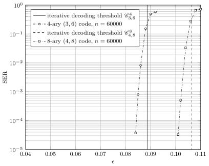
Figure 1: SER vs. channel error probability $\epsilon$ for a $4$-ary $(3,6)$ LDPC code and a $8$-ary $(4,8)$ LDPC code with $n=60000$.

Fig. 1 compares the iterative decoding threshold for the $\mathscr{C}_{3,6}^{4}$ and $\mathscr{C}_{4,8}^{8}$ LDPC code ensembles with the symbol error rate (SER) of a $4$-ary $(\mathsf{d_{v}}=3,\mathsf{d_{c}}=6)$ and $8$-ary $(\mathsf{d_{v}}=4,\mathsf{d_{c}}=8)$ LDPC code, respectively, with $n=60000$. The SER results were obtained by Monte Carlo simulations and $200$ decoding iterations. As expected, the iterative decoding threshold predicts accurately the waterfall performance of the codes.

VI Conclusions

We presented symbol message passing, a low-complexity decoding algorithm for $q$-ary LDPC codes. A DE analysis is presented for regular ensembles over the $q$-SC. It yields iterative decoding thresholds and message weights which result in performance advantages with respect to a competing scheme of similar complexity. We also derived tight upper and lower bounds on the VN message error probabilities, which allow efficient and accurate computation of the thresholds.

Efficient Evaluation of Density Evolution

We derive tight upper and lower bounds on (17), which can be efficiently evaluated. For the sake of simplicity, whenever possible we drop the iteration count in the following. Let ${\mu}_{j}(\bm{F})$ denote the number of elements of $\bm{F}$ equal to $j$, i.e.,

$${\mu}_{j}(\bm{F})=\left|\left\{F_{a},a\in\mathbb{F}_{q}\big{|}F_{a}=j\right\}\right|.$$ (18)

Let us define ${t_{b}}$ as

$${t_{b}}=f_{b}+\frac{\mathsf{D}(\epsilon)}{\mathsf{D}(\xi)}$$

where we consider channels with non-zero capacity, i.e., $\mathsf{D}(\cdot)>0$. Let VN $\mathtt{v}$ receive a channel message $y=0$, and $f_{0}$ messages with value $0$ from its neighbors. Whenever

$$\max_{i\in\mathbb{F}_{q}\setminus 0}(F_{i})<{t_{0}}$$

the outgoing VN-to-CN message will be $0$. Further, whenever

$$\max_{i\in\mathbb{F}_{q}\setminus 0}(F_{i})={t_{0}}$$

the outgoing VN-to-CN message will take value $0$ with probability 1$/{\mu}_{{t_{0}}}(\bm{F})$. Similar considerations can be made when $y\neq 0$. Thus, for $q>2$, we may recast (17). This yields (29), where

$$\kappa_{\mathrm{max}} =\min\left(\Big{\lfloor}\frac{\mathsf{d_{v}}-1-f_{0}}{{t_{0}}}\Big{\rfloor},q-1\right)$$ (19)

$$\kappa_{\mathrm{max}}^{\prime} =\min\left(\Big{\lfloor}\frac{\mathsf{d_{v}}-1-f_{1}}{f_{0}}\Big{\rfloor},q-1\right)$$ (20)

$$\kappa_{\mathrm{max}}^{\prime\prime} =\min\left(\Big{\lfloor}\frac{\mathsf{d_{v}}-1}{{t_{1}}}\Big{\rfloor},q-1\right).$$ (21)

$$p_{0}^{(\ell)} =p_{0}^{(0)}\sum_{f_{0}=0}^{\mathsf{d_{v}}-1}P_{F_{0}|X}(f_{0}|0)\Bigg{(}\Pr\left\{\max_{i\in\mathbb{F}_{q}\setminus 0}(F_{i})<{t_{0}}\big{|}X=0,F_{0}=f_{0}\right\}\hfill$$ (22)

$$+\Pr\left\{\max_{i\in\mathbb{F}_{q}\setminus 0}(F_{i})={t_{0}}\big{|}X=0,F_{0}=f_{0}\right\}\underbrace{\sum_{\kappa=1}^{\kappa_{\mathrm{max}}}\frac{1}{\kappa+1}\Pr\left\{{\mu}_{{t_{0}}}(\bm{F})=\kappa\big{|}X=0,F_{0}=f_{0},\max_{i\in\mathbb{F}_{q}\setminus 0}(F_{i})={t_{0}}\right\}}_{\text{(a)}}\Bigg{)}$$ (23)

$$+(q-1)\,p_{1}^{(0)}\sum_{f_{1}=0}^{\mathsf{d_{v}}-1}P_{F_{1}|X}(f_{1}|0)\Bigg{[}\sum_{f_{0}>{t_{1}}}^{\mathsf{d_{v}}-1-f_{1}}P_{F_{0}|X,F_{1}}(f_{0}|0,f_{1})\Bigg{(}\Pr\left\{\max_{i\in\mathbb{F}_{q}\setminus\{0,1\}}(F_{i})<f_{0}\big{|}X=0,F_{0}=f_{0},F_{1}=f_{1}\right\}$$ (24)

$$+\Pr\left\{\max_{i\in\mathbb{F}_{q}\setminus\{0,1\}}(F_{i})=f_{0}\bigg{|}X=0,F_{0}=f_{0},F_{1}=f_{1}\right\}$$ (25)

$$\times\underbrace{\sum_{\kappa=2}^{\kappa_{\mathrm{max}}^{\prime}}\frac{1}{\kappa}\Pr\left\{{\mu}_{f_{0}}(\bm{F})=\kappa\bigg{|}X=0,F_{0}=f_{0},F_{1}=f_{1},\max_{i\in\mathbb{F}_{q}\setminus\{0,1\}}(F_{i})=f_{0}\right\}}_{\text{(b)}}\Bigg{)}$$ (26)

$$+P_{F_{0}|X,F_{1}}({t_{1}}|0,f_{1})\Bigg{(}\frac{1}{2}\Pr\left\{\max_{i\in\mathbb{F}_{q}\setminus\{0,1\}}(F_{i})<{t_{1}}\bigg{|}X=0,F_{0}={t_{1}},F_{1}=f_{1}\right\}$$ (27)

$$+\Pr\left\{\max_{i\in\mathbb{F}_{q}\setminus\{0,1\}}(F_{i})={t_{1}}\bigg{|}X=0,F_{0}={t_{1}},F_{1}=f_{1}\right\}$$ (28)

$$\times\underbrace{\sum_{\kappa=2}^{\kappa_{\mathrm{max}}^{\prime\prime}}\frac{1}{\kappa+1}\Pr\left\{{\mu}_{{t_{1}}}(\bm{F})=\kappa\bigg{|}X=0,F_{0}={t_{1}},F_{1}=f_{1},\max_{i\in\mathbb{F}_{q}\setminus\{0,1\}}(F_{i})={t_{1}}\right\}}_{\text{(c)}}\Bigg{)}\Bigg{]}$$ (29)

An upper bound on $p_{0}^{(\ell)}$ is obtained as follows. Whenever the aggregated $\bm{L}$-vector $\bm{E}^{(\ell)}$ has $\kappa>1$ maxima, one of them being at $0$, we assume that $\bm{E}^{(\ell)}$ has the minimum possible number of maxima. We thus replace the terms (a), (b), (c) in (29) by $1/2$, $1/2$, and $1/3$, respectively. Similarly, a lower bound can be obtained by replacing the terms (a), (b), (c) in (29) by $1/(\kappa_{\mathrm{max}}+1)$, $1/\kappa_{\mathrm{max}}^{\prime}$, and $1/(\kappa_{\mathrm{max}}^{\prime\prime}+1)$, respectively. For the lower bound we thus overestimate the number of maxima. Both upper and lower bounds can be efficiently evaluated using a result in [19]. Both bounds are tight for the ensembles in Tables LABEL:table:3:5:qsc and LABEL:table:3:6:qsc. In fact, they coincide in the first $6$ decimal digits.

References

- [1] R. G. Gallager, “Low-density parity-check codes,” Ph.D. dissertation, Dep. Electrical Eng., M.I.T, Cambridge, MA, Jul. 1963.
- [2] T. Richardson and R. Urbanke, “The capacity of low-density parity-check codes under message-passing decoding,” IEEE Trans. Inf. Theory, vol. 47, no. 2, pp. 599–618, Feb. 2001.
- [3] G. Lechner, T. Pedersen, and G. Kramer, “Analysis and design of binary message passing decoders,” IEEE Trans. Commun., vol. 60, no. 3, pp. 601–607, Mar. 2012.
- [4] E. B. Yacoub, F. Steiner, B. Matuz, and G. Liva, “Protograph-based LDPC code design for ternary message passing decoding,” in Proc. ITG Int. Conf. Syst., Commun. and Coding, Rostock, Germany, Feb. 2019.
- [5] S. K. Planjery, D. Declercq, L. Danjean, and B. Vasic, “Finite alphabet iterative decoders – part i: Decoding beyond belief propagation on the binary symmetric channel,” IEEE Trans. Commun., vol. 61, no. 10, pp. 4033–4045, Oct. 2013.
- [6] M. Davey and D. MacKay, “Low density parity check codes over GF,” IEEE Commun. Lett., vol. 2, no. 6, pp. 70–71, Jun. 1998.
- [7] L. Barnault and D. Declercq, “Fast decoding algorithm for LDPC over GF(),” in Proc. IEEE Inf. Theory Workshop (ITW), Cergy, France, Mar. 2003, pp. 70–73.
- [8] D. Declercq and M. Fossorier, “Decoding algorithms for nonbinary LDPC codes over GF (),” IEEE Trans. Commun., vol. 55, no. 4, pp. 633–643, Apr. 2007.
- [9] J. J. Metzner, “Majority-logic-like decoding of vector symbols,” IEEE Trans. Commun., vol. 44, no. 10, pp. 1227–1230, Oct. 1996.
- [10] M. G. Luby and M. Mitzenmacher, “Verification-based decoding for packet-based low-density parity-check codes,” IEEE Trans. Inf. Theory, vol. 51, no. 1, pp. 120–127, Jan. 2005.
- [11] B. Matuz, G. Liva, E. Paolini, and M. Chiani, “Verification-based decoding with map erasure recovery,” in Proc. ITG Int. Conf. Syst. Commun. and Coding, München, Germany, Jan 2013.
- [12] A. Shokrollahi and W. Wang, “Low-density parity-check codes with rates very close to the capacity of the q-ary symmetric channel for large q,” in Proc. IEEE Int. Symp. on Inf. Theory, Jun. 2004, p. 273.
- [13] F. Zhang and H. D. Pfister, “Analysis of verification-based decoding on the -ary symmetric channel for large ,” IEEE Trans. Inf. Theory, vol. 57, no. 10, pp. 6754–6770, 2011.
- [14] B. M. Kurkoski, K. Yamaguchi, and K. Kobayashi, “Density evolution for GF() LDPC codes via simplified message-passing sets,” in Proc, IEEE Inf. Theory and Appl. Workshop, 2007, pp. 237–244.
- [15] M. Stark, G. Bauch, J. Lewandowsky, and S. Saha, “Decoding of non-binary LDPC codes using the information bottleneck method,” in Proc. IEEE Int. Conf. on Commun., 2019.
- [16] R. Misoczki, J. Tillich, N. Sendrier, and P. S. L. M. Barreto, “MDPC-McEliece: New McEliece variants from moderate density parity-check codes,” in Proc of IEEE Intern. Symp. on Inf. Theory, Jul. 2013.
- [17] A. Ashikhmin, G. Kramer, and S. ten Brink, “Extrinsic information transfer functions: model and erasure channel properties,” IEEE Trans. Inf. Theory, vol. 50, no. 11, pp. 2657–2673, Nov. 2004.
- [18] F. Lázaro, G. Liva, E. Paolini, and G. Bauch, “Bounds on the error probability of Raptor codes under maximum likelihood decoding,” arXiv preprint arXiv:1809.01515, 2018.
- [19] B. Levin, “A representation for multinomial cumulative distribution functions,” The Annals of Statistics, vol. 9, no. 5, pp. 1123–1126, 1981.