Boosting Operational DNN Testing Efficiency through Conditioning
Abstract.
With the increasing adoption of Deep Neural Network (DNN) models as integral parts of software systems, efficient operational testing of DNNs is much in demand to ensure these models’ actual performance in field conditions. A challenge is that the testing often needs to produce precise results with a very limited budget for labeling data collected in field.
Viewing software testing as a practice of reliability estimation through statistical sampling, we re-interpret the idea behind conventional structural coverages as conditioning for variance reduction. With this insight we propose an efficient DNN testing method based on the conditioning on the representation learned by the DNN model under testing. The representation is defined by the probability distribution of the output of neurons in the last hidden layer of the model. To sample from this high dimensional distribution in which the operational data are sparsely distributed, we design an algorithm leveraging cross entropy minimization.
Experiments with various DNN models and datasets were conducted to evaluate the general efficiency of the approach. The results show that, compared with simple random sampling, this approach requires only about a half of labeled inputs to achieve the same level of precision.
1. Introduction
Deep Learning has gained great success in tasks that are intuitive to human but hard to describe formally, such as image classification or speech recognition (LeCun et al., 2015; Goodfellow et al., 2016). As a result, Deep Neural Networks (DNNs) are increasingly adopted as integral parts of widely used software systems, including those in safety-critical application scenarios such as medical diagnosis (Obermeyer and Emanuel, 2016) and self-driven cars (Pei et al., 2017). Effective and efficient testing methods for DNNs are thus needed to ensure their service quality in operation environments.
Recent efforts on DNN testing (Ma et al., 2018a; Pei et al., 2017; Sun et al., 2018a; Ma et al., 2018d; Sun et al., 2018b; Odena and Goodfellow, 2018; Zhang et al., 2018) have aimed at generating artificial adversarial examples, which resembles the debug testing (Frankl et al., 1998) of human written programs that aims at finding error-inducing inputs. However, the fundamental difference between DNN models and human written programs challenges the basic concepts and wisdoms for debug testing. For example, the inductive nature of statistical machine learning and the No-Free-Lunch theorem imply that an oracle for a DNN model independent of its operation context is senseless. The fact that DNN performance is measured statistically also diminishes the importance of individual error-inducing inputs.
Contrastingly, this paper focuses on the operational testing of DNN, i.e., testing a previously trained DNN model with the data collected from a specific operation context, in order to determine the model’s actual performance in this context. Although operational testing for conventional software has been extensively studied (Musa, 1993; Frankl et al., 1998; Lyu, 2007), the challenge of operational DNN testing is not well understood in the software engineering community. A central problem here is that it can be prohibitively expensive to label all the operational data collected in field. For example, a surgical biopsy may be needed to decide whether a radiology or pathology image is really malignant or benign. In this case the labeling effort for each single example is worth saving. Thus it is crucial to test DNN efficiently, i.e., to precisely estimate a DNN’s actual performance in an operation context, but with a limited budget for labeling data collected from this context.
We propose to reduce the number of labeled examples required in operational DNN testing through carefully designed sampling. The conventional wisdom behind structural coverages for testing human written programs is re-interpreted in statistical terms as conditioning for variance reduction, and applied to the sampling and estimation of DNN’s operational accuracy.
The key insight is that, the representation learned by a DNN and encoded in the neurons in the last hidden layer can be leveraged to guide the sampling from the unlabeled operational data. It turns out that conditioning on this representation is effective, and works well even when the model is not well-fitted to the operation data, which is a property not enjoyed by naive choices such as stratifying by classification confidence.
To realize the idea, one must select a small fraction from the operational data, but with sufficient representativeness in terms of their distribution in the space defined by the outputs of neurons in the last hidden layer. This is difficult because the space is high-dimensional, and in which the operational data themselves are sparsely distributed. We solve this problem with a distribution approximation technique based on cross-entropy minimization.
The contributions of this paper are:
-
•
A formulation of the problem of operational DNN testing as the estimation of performance with a small sample, and a proposal for efficient testing with variance reduction through conditioning, as a generalization of structural coverages.
-
•
An efficient approach to operational DNN testing that leverages the high dimensional representation learned by the DNN under testing, and a sampling algorithm realizing the approach based on cross entropy minimization.
-
•
A systematic empirical evaluation. Experiments with LeNet, VGG, and ResNet show that, compared with simple random sampling, this approach requires only about a half of labeled inputs to achieve the same level of precision.
The rest of this paper is organized as follows. In Section 2 we discuss the problem of operational DNN testing and how to improve its efficiency. Section 3 is devoted to the conditioning approach to efficient DNN testing, and Section 4 to the empirical evaluation of the approach. We then review related work in Section 5, before concluding the paper with Section 6.
2. Operational Testing of DNNs
In this section we briefly introduce DNN, examine the problem of testing DNNs as software artifacts in operation context, and then discuss the insights for and the challenges to efficient DNN testing.
2.1. Deep Neural Network
A deep neural network (DNN) is an artificial neural network (ANN) with multiple intermediate (hidden) layers. It encodes a mathematical mapping from inputs to outputs with a cascading composition of simple functions implemented by the neurons. Figure 1 is a simple example of neural network. The existence of activation functions makes the model nonlinear.
To approximate the intricate mapping hidden in the training examples, a DNN model has its parameters (weights and biases ) gradually adjusted to minimize the averaged prediction error over all the examples. What a DNN actually learned is a posterior probability distribution, denoted as . For example, for a k-classification problem, DNN will give k posterior probability functions for the given input . The predicted label for this input is the class corresponding to the maximum posteriori probability, i.e. .
2.2. The DNN Testing Problem
When a previously trained DNN model is adopted as an integral part of a software system deployed in a specific environment, it may drastically underperform its expected accuracy. There can be different causes, such as under-fitting or over-fitting of the model to the training data set, or the data distribution discrepancy between the training set and the data emerged in the operation context. The latter is especially nasty and often encountered in practice. Therefore, as any software artifact, a DNN model must be sufficiently tested before being put into production.
DNN testing is different from traditional software testing aiming at identifying error-inducing inputs. DNN implements a kind of inductive reasoning, which is fundamentally different from human written programs based on logic deductions. As a consequence, for a trained DNN there does not exist a certain and universal oracle for testing. Elaborately, the testing of DNNs has to be
- Statistical:
-
Contrasting to human written programs with certain intended behaviors, as a statistical machine learning model, a DNN offers only some probabilistic guarantee, i.e., to make probably correct prediction on most inputs it concerns (Goodfellow et al., 2016). In fact, mispredictions on a small portion of inputs are expected, and in some sense intentional, in order to avoid overfitting and maximizing generality.
- Holistic:
-
Up to now there is no viable rationale interpretation of DNNs’ internal behaviors on individual inputs at the level of neurons (Abid et al., 2019; Lipton, 2016). This means that DNNs are essentially blackboxes although their computation steps are visible. Also, a detected fault with a specific input is hardly helpful for “debugging” the DNN.
- Operational:
So generally the task of testing a DNN as a software component is, giving a previously trained DNN model and a specific operation context, to decide how well the model will perform in this context, which is expressed statistically with the estimated accuracy of prediction111In this paper we consider only accuracy that is the proportion of examples for which the model predicts correctly. However, the proposed method is generally applicable to other performance measures.. This task should be easy if we had enough labeled data that well represent the operation context and suffice accurate estimation. However, in practice, although unlabeled data can be collected from the operation environment, labeling them with high-quality is often expensive.
For example, considering an application scenario of AI-aided clinical medicine (Obermeyer and Emanuel, 2016) where a hospital is going to adopt a DNN model to predict MRI images to be malignant or benign. Suppose that the model is previously trained by a foreign provider with its proprietary dataset, and thus the hospital needs to gauge it against native patients and local equipment settings. The hospital may collect a lot of images by scanning patients and volunteers, but labeling them is much more expensive because not only advanced human expertise, but also some complicated laboratory testings and even intrusive biopsies are required.
Therefore, a central problem of DNN testing is how to accurately estimate DNNs’ performance in their operational context with small-size samples222There is a common mistake of regarding a sample of more than 30 elements as large enough (Beleites et al., 2013). As we will see in Section 4, we often need much more. of labeled data. Or in other words, given a budget of cost in labeling examples, how to make the estimation of a DNN’s performance as accurate as possible.
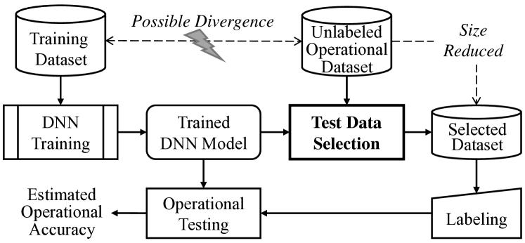
Figure 2 illustrates the process of efficient operational DNN testing. The goal is that, with some sophisticated test data selection, one only needs to label a small portion of operational data to achieve enough precision for the estimation of operational accuracy.
2.3. Improving Testing Efficiency through Conditioning
Clearly, the above description of DNN testing resembles statistical sampling and estimation, whose efficiency can be improved with variance reduction techniques (Owen, 2013). In the following we briefly introduce the simple random sampling as the baseline estimation method, and then discuss how conditioning can help with some inspirations from the coverage-oriented testing of conventional programs.
Sampling is the process of selecting a group of individuals from a population in order to study them and estimate the property of population. Specifically, suppose that there is a fixed parameter that needs to be estimated, where is a random variable corresponding to the observed data, and is the model of interest. For example, when estimating the accuracy of a DNN model, is defined as if the DNN correctly predicts ’s label, and otherwise. Note that is also a random variable. An estimator of is denoted by the symbol .
The basic sampling method is Simple Random Sampling (SRS). SRS draws i.i.d. replications directly from the population. The i.i.d. condition requires that each individual is chosen randomly and entirely by chance, such that each individual has the same probability of being chosen, and each set of individuals has the same probability of being chosen for the sample as any other set of individuals. And the estimator is computed as the average of each estimate:
| (1) |
This is an unbiased estimator, i.e. . The efficiency of SRS is expressed statistically by its variance .
Despite of its simplicity, SRS is quite effective in practice if we can draw a sufficiently large i.i.d. sample. Without further information about we can hardly improve over SRS. An often used strategy is conditioning, i.e., to find a random variable or vector , on which ideally strongly depends, and leverage the law of total variance:
| (2) |
Intuitively, the law says if we “interpret” with , the variance of can be decomposed to those not explained by (the first term on the right hand), and those due to (the second term). Note that itself is a function on , and
| (3) |
So we can sample from ’s distribution and estimate instead of , taking the advantage that the former has a smaller variance than the latter.
If we can make a complete sample of , i.e., covering all possible values for , the variance of our estimation will be only those introduced in estimating for each . This is exactly what Stratified Sampling does. Furthermore, if the value of is fully determined by , we will have zero variance.
These two ideal conditions are hard to satisfy, especially in complex scenarios such as operational software testing. However, the insights are clear: to improve the efficiency of testing as estimation, we need
-
(1)
to identify an observable factor that affects the performance (accuracy) as much as possible, so that the variance of conditioned under each is minimized, and
-
(2)
to draw as representative as possible samples for , so that the uncertainty due to can be well handled.
These two aspects can be conflicting in practice. Intuitively, the more “precise” the interpretation for is, the finer grained it has to be, and the harder it can be sufficiently represented by a small-size sample. It is crucial to strike a good balance between them with a deliberately chosen .
It is inspiring to use this viewpoint to examine the structural coverage-directed testing of conventional programs, despite of the difference that structural coverages are mainly used to identify error-inducing inputs. The efficacy of a structural coverage comes from
-
(1)
the homogeneity of inputs covering the same part of a program – either all or none of them induces an error, so that testing efficiency can be improved by avoiding duplications, and
-
(2)
the diversity of inputs indicated by coverage metrics, so that testing completeness can be improved by enforcing a high coverage to touch corner cases in which rare errors may hide.
Evidently, these two heuristics resemble the two insights of conditioning.
In this sense, the conditioning techniques for testing efficiency improvement can be regarded as a generalization of structural coverages in conventional white-box software testing. However, it turns out to be challenging to apply this idea to the testing of DNNs, because of
-
(1)
the blackbox nature of DNNs. There is no obvious structural features like program branches or execution paths of human written programs that intuitively provide the needed homogeneity, and moreover,
-
(2)
the curse of dimensionality. For DNNs, a powerful interpreting factor for model accuracy is often a high dimensional vector, which makes it very difficult to represent with a small-size sample but without huge uncertainty.
We will discuss how to meet these challenges in the next section.
3. Efficient DNN testing methods
First, let us state our problem of efficient operational DNN testing more specifically:
Problem 0.
Given a trained DNN model, and a set of unlabeled examples collected from an operation context, instead of labeling all these examples, select and label a subset with a given size budget , and use to estimate the accuracy of on , with an as small estimation error as possible.
Leveraging the information provided by and , we try to achieve efficient estimation through conditioning. We first discuss Confidence-based Stratified Sampling (CSS), which is simple but unfortunately fragile and limited to classifiers. Then we present Cross Entropy-baed Sampling (CES) that conditions on representations learned by , and approximates the distribution of through cross-entropy minimization.
3.1. Confidence-based Stratified Sampling
As discussed earlier, the key to improve the estimation efficiency is to find a random variable that is strongly correlated to the accuracy of the model , and whose distribution is easy to sample. A natural choice is the confidence value provided by some classifier models when predicting the label for . Obviously, predictions with a higher confidence will be more likely to be correct, if the classifier is reliable.
Since the confidence is a bounded scalar, we can divide its range into sections, and stratify the population into strata accordingly. Thus the probability of an example belonging to is , . From each stratum , randomly taking elements such that . Then the accuracy of on is estimated as
| (4) |
A simple strategy is to use proportional allocation, i.e., , and then the estimation of accuracy becomes . However, although safe (Chen et al., 2001), proportional allocation may be suboptimal.
The variance of a stratified estimator is the sum of variances in each strata: . It can be further reduced if we allocate more examples in strata that are less even. Specifically, we can guess that a stratum with a lower confidence should fluctuate more in the accuracy. So we should take more examples from those low-confidence strata.
The optimal stratification and example allocation depend on the actual distribution of the variance of conditioned on the confidence, which is not known a priori. They have to be determined according to experience and pilot experiments.
Unfortunately, CSS is not robust for operational DNN testing. It performs very well when the model is perfectly trained for the operation context. However, as shown in our experiments reported in Section 4, when the model is not well-fitted to the operational data set, its performance drops drastically. Note that this unfavorable situation is the motivation for operational DNN testing. It is not difficult to see the reason – when the model predicts poorly in the operation context, the confidence values it produces cannot be trusted. In addition, confidence values are not readily available in regression tasks. Therefore, we propose another variance reduction method based on behaviors of neurons.
3.2. Cross Entropy-based Sampling
A better choice for the condition random variable is the output of neurons in the last hidden layer. It is often viewed as a learned representation of the training data that makes the prediction easier (Goodfellow et al., 2016, p. 6 and p. 518). The rationale behind this choice is manifold. First, although not necessarily comprehensible for human, the representation is more stable than the prediction when the operation context is drifting. This is supported by well-known transfer learning practices where only the SoftMax layer is retrained for different tasks (Huang et al., 2013). Second, the DNN prediction is directly derived from the linear combination of this layer’s outputs, and thus it must be highly correlated with the prediction accuracy. Finally, the correlation between the neurons in this layer is believed to be smaller than those in previous layers (Bengio et al., 2013), which facilitates the approximation of their joint distribution that will be used in our algorithm.
For a trained DNN model we consider its last hidden layer consisting of neurons denoted by . We divide , the output range of each neuron , into equal sections , and define function if the output of for input belongs to , .
Hence the conditional variable is a vector , , . Let be a subset of whose elements are mapped onto by the model. The probability distribution of is defined with the operational data set as
| (5) |
However, considering the high dimensionality of , it is challenging to take a typical sample from the whole test set according to ’s distribution, not to mention applying stratified sampling. Note that we cannot use artificial examples generated according to ’s distribution because we need to evaluate the model’s accuracy on real data in the given operation context. Now the problem is how to select a small-size sample from a finite population which itself is sparsely distributed in a high dimensional space, such that the sample is as “representative” as possible for the population.
To this end, we propose to select a typical333cf. Shannon’s concept of typical set (MacKay and Mac Kay, 2003; Ho and Yeung, 2010). sample by minimizing the cross entropy (Goodfellow et al., 2016) between and :
| (6) | ||||
where
| (7) |
In this high-dimensional case, the minimization is hard to compute directly, partially because of the sparseness of and in ’s space. Fortunately, it is observed that a DNN typically reduces the correlation among neurons in the last hidden layer (Koller et al., 2009), thus we can take an approximation by assuming that they are independent of each other in computing the minimization. In this case we can minimize through minimizing the average of the cross entropy between and on each dimension:
| (8) |
where
| (9) |
and is defined similarly.
Furthermore, the optimal solution of is achieved when (Shore and Johnson, 1980). Therefore, the estimator for model accuracy is given by:
| (10) | ||||
Note that this estimator is unbiased according to Equation 3.
To solve the optimization problem of Equation 8, we propose an algorithm (Algorithm 1) similar to random walk (Révész, 2005). Elaborately, we first randomly select examples as the initial sample set , and repeatedly enlarge the set by a group of examples until we exhaust the budget of . At each step, is selected from randomly selected groups, minimizing the cross entropy.
| (11) |
Finally, there is an intrinsic connection between structural coverage and the cross entropy in Equation 6. Structural coverages actually assume the probability of to be a constant. In this case, minimizing becomes maximizing , which equals to maximizing . Since , it is to even the distribution , which is actually to maximize the coverage so that more instances of are covered.
4. Evaluation
Cautious readers may have noted that our approach leverages several heuristics and approximations, including the stableness of the representation learned by a DNN model despite of the possible drift of its operational data, the independence between the outputs of neurons in the last hidden layer, and the optimization through random walk in Algorithm 1. Thus, a systematic empirical evaluation is needed to validate the general efficacy of the approach.
In the following, we first briefly introduce the implementation of our CSS and CES approaches, then discuss some different situations faced by operational DNN testing, and how experiments are designed accordingly. After that we present the results of the experiments, which unanimously confirm that our approach greatly improves testing efficiency.
4.1. Implementation
We implemented our approach using Tensorflow 1.12.0 and Keras 2.2.4 DL frameworks. The code, along with additional experiment results444Besides those discussed this Section, additional experiments were carried out to validate the superiority of the last hidden layer over other layers as the learned representation to condition on in CES, to explore whether the surprise value (Kim et al., 2019) can be used as an alternative for the confidence in CSS, and to examine the relative efficiency of CES over SRS with relatively bigger samples. Due to the page limit, we cannot include them in this paper., can be found at https://github.com/Lizenan1995/DNNOpAcc.
For CSS, we use an optimal setting achieved through pilot experiments. The population is partitioned into three strata. The 80% examples of the whole operational dataset with the highest confidence are assigned to the first stratum, the next 10% to the second stratum, and the lowest 10% to the third stratum. To draw a sample with size , we take , , and examples from the three strata, respectively.
For the CES approach that conditions on representation, we set the number of sections for each neuron to . This is not necessarily the best number, but is reasonable considering the tens-to-few-hundreds examples are expected to be sampled. In implementing Algorithm 1, we select initial examples, and enlarge the set by examples in each step. The number of random groups examined in each step is set to . These parameters are fixed in all experiments except for those with very small operational test sets (to be detailed in Section 4.3.4). Further optimizations of these parameters is possible, but the above values are already sufficient for achieving a significant efficiency improvement over SRS.
4.2. Experiment Design
Generally, operational DNN testing is to detect the performance loss of a DNN model when used in a specific operation context. Here we assume that the model is well trained with its training set, and do not explicitly consider the problems usually addressed in the training process, such as under-fitting or over-fitting. Hence the performance loss is likely to be caused by
-
•
Polluted training set. The training set is mutated by an accident or malicious attack, and thus a mutated model is generated.
-
•
Different system settings. For example, the model might be trained with high-resolution examples but used to classify low-resolution images due to the limitation of the camera equipped in the system.
-
•
Different physical environment. For example, the lightening condition may vary in the operation environment.
In addition, we need to consider the differences in the purpose (classification or regression), the scale of DNN models, and the size of unlabeled operational test sets.
With these considerations, as shown in Table 1, we designed 20 experiments in total, which varied in the training sets, the DNN models, the operational testing sets and thus the actual operational accuracies. DNN models with very different structures were used in these experiments. Table 2 lists the numbers of their layers and neurons.
| No. | Train | Model | Operational | Actual | E-Value |
| Set | Test Set | Acc. (%) | CES/SRS | ||
| 1 | MNIST | LeNet-1 | MNIST | 93.1 | 0.588 |
| 2 | LeNet-4 | 96.8 | 0.655 | ||
| 3 | LeNet-5 | 98.7 | 0.708 | ||
| 4 | Mutant1a | 79.5 | 0.499 | ||
| 5 | Mutant2a | 77.3 | 0.380 | ||
| 6 | Mutant3a | 79.1 | 0.478 | ||
| 7 | Driving | Dave-orig | Driving | 90.4b | 0.592 |
| 8 | Dave-drop | 91.8b | 0.588 | ||
| 9 | Dave-orig | patch | 88.3b | 0.426 | |
| 10 | Dave-drop | 83.5b | 0.526 | ||
| 11 | Dave-orig | light | 89.8b | 0.375 | |
| 12 | Dave-drop | 88.5b | 0.481 | ||
| 13 | ImageNet | VGG-19 | ImageNet | 72.7 | 0.567 |
| 14 | ResNet-50 | 75.9 | 0.471 | ||
| 15 | VGG-19 | resolution | 63.3 | 0.470 | |
| 16 | ResNet-50 | 68.8 | 0.436 | ||
| 17 | Mutant1a | LeNet-5 | MNIST-100 | ||
| 18 | MNIST-300 | ||||
| 19 | Driving | Dave-orig | patch-100 | ||
| 20 | patch-300 |
-
a
The three mutated models are trained by changing the labels of training data: , , , respectively.
-
b
Since the steering angle is a continuous value, we use 1-MSE (Mean Squared Error) as the accuracy.
-
c
It is the mean value of 30 experiments with different randomly selected test sets.
| Model | LeNet- | DAVE- | VGG-19 | ResNet-50 | |||
| 1 | 4 | 5 | orig | drop | |||
| Neurons | 52 | 148 | 268 | 1,560 | 844 | 16,168 | 94,059 |
| Layers | 7 | 8 | 9 | 13 | 15 | 25 | 176 |
The first group of experiments (No.1-6, results to be discussed in Section 4.3.1 ) were designed to study the effect of a polluted training set, and to see whether the conditioning approaches were robust when the actual accuracy varied. The second group of experiments (No.7-12, Section 4.3.2) simulated different physical environment conditions, and the third group (No.13-16, Section 4.3.3) were for different system settings.
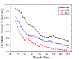
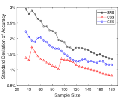
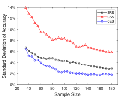
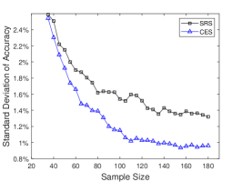
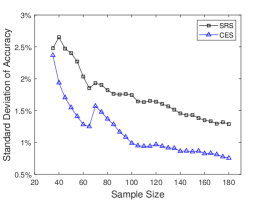
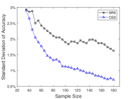
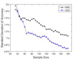
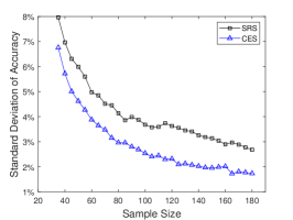
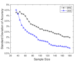
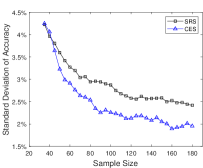
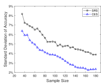
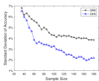
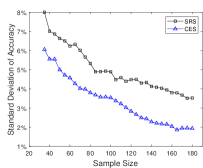
In these experiments, we compared the mean squared errors of different estimated accuracy from different estimators. They were the SRS estimator (Section 2.3), the CSS estimator (Section 3.1), and the CES estimator (Section 3.2). Each experiment was repeated 50 times on each sample size of .555Focusing on estimation with small size samples, here we only give results up to sample size 180. However, an additional experiment presented at our code website demonstrated that the relative efficiency of CES over SRS is quite stable when the sample size grew up to 2500. The mean square error was computed as , where and were the estimated and actual operational accuracy, respectively. Note that because all these estimators are unbiased, the can be regarded as the estimation variance, whose square root, i.e., the standard deviation, is plotted in the Figures 3, 4, and 7.



The final group of experiments (No. 17-20, Section 4.3.4) were designed to see whether our approach still worked in cases that only a small number of unlabeled operational examples were available. We tested cases of taking a sample of size 30 from an operational test set of size 100, and of taking a sample of 50 from 300.
In addition to the visual plotting of standard deviations, we also computed the relative efficiency of two estimators as the ratio between their variances. Considering that the variance of an SRS estimator is inversely proportional to the sample size, actually indicates the rate of sample size reduction. We list the averaged values (the smaller the better) of CES to SRS for each experiment in the last column of Table 1.
Experiments with the ImageNet dataset (No. 13-16) were conducted on a Linux server with two 10-core 2.20GHz Xeon E5-2630 CPUs, 124 GB RAM, and 2 NVIDIA GTX 1080Ti GPUs, and other experiments were on a Linux laptop with an 2.20GHz i7-8750H CPU, 16 GB RAM, and a NVIDIA GTX 1050Ti GPU. For a feeling about the computational cost of sampling with CES, we observed that, to select out a sample of size 100, it took 8.27s for MNIST/LeNet-5, 20.50s for Driving/Dave-orig, and 420.09s for ImageNet/VGG-19.
4.3. Experiment Results
4.3.1. Experiments with the MNIST dataset
Experiments 1-6 were conducted on the MNIST dataset (LeCun et al., 1998) that is widely used in machine learning research. It is a handwritten digit dataset consisting of 60,000 2828-pixel training images and 10,000 testing images in 10 classes. With this dataset, we trained three LeNet family models (LeNet-1, LeNet-4, and LeNet-5) (LeCun et al., 1998).
Experiments 1-3 tested the ideal situation where the training set and testing set were both original. Experiments 4-6 the models were trained with mutated training set, but tested with the original testing images as the operational dataset. The mutated training set is obtained by exchanging the labels of training data.
From the first row of Figure 3 we can see that, when there was no divergence between the training data and the operational data, the CSS estimator performed particularly well, achieving a , , and average efficiency relative to SRS for the three models tested, respectively. However, the second row of Figure 3 tells a completely different story. In this case, the training set had been mutated, and CSS performed very bad, with a , , and average relative efficiency, respectively. Clearly, the CSS estimator is not robust to the divergence between the training data and operational data.
On the contrary, the CES estimator consistently outperformed SRS in both cases. From Figure 3 and the relative efficiency values listed in Table 1, we can see that CES only required about a half of labeled data to achieve the same level of precision of estimation.
The result of Experiment 3 also suggests that, when the operational accuracy was very high (about 99%), the benefit of our CES diminished, to a level saving about 30% labeling effort. However, this should not be a problem because the accuracy is high, and in this situation we can switch to CSS if needed.
4.3.2. Experiments with the Driving dataset
The next 6 experiments were conducted on the Driving dataset666https://udacity.com/self-driving-car. It is the Udacity self-driving car challenge dataset containing 101,396 training and 5,614 testing examples. This is a regression task that predicts the steering wheel angle based on the images captured by a camera equipped on a driving car. Two pre-trained DNNs (DAVE-orig and DAVE-dropout (Bojarski et al., 2016)) were used in our experiments.


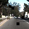
Experiments 7 and 8 tested the ideal situation where the operational test set is untouched. Experiments 9-12 used mutated operational data simulating unideal physical environment conditions, with the two methods used by DeepXplore (Pei et al., 2017): occlusion by small rectangles simulating an attacker blocking some parts of a camera (Experiments 9 and 10) and lighting effects for simulating different intensities of lights (Experiments 11 and 12). Figure 5 illustrates the mutations.
Figure 4 plots the mean squared errors of CES and SRS for each of the 6 experiments. Because the regression models did not provide confidence values, the CSS estimator could not be applied in these experiments.
The results show that CES also worked well for regression tasks, and achieved 0.375-0.526 relative efficiency w.r.t. SRS when divergence between training data and operational data existed.
4.3.3. Experiments with the ImageNet dataset
The ImageNet (Deng et al., 2009) dataset is chosen for the last 4 experiments. It is a large collection of more than 1.4 million images as the training data and other 50,000 as the test data, in 1,000 classes. Two large scale pre-trained models, viz. VGG-19 (Simonyan and Zisserman, 2014) and ResNet-50 (He et al., 2015) were taken as the subject.
Again, Experiments 13 and 14 used the original test set as the operational data. Experiments 15 and 16 used low resolution images as the operational testing data, which were obtained by downsampling the images in the original test set, as shown in Figure 6.


The results of these experiments, as shown in Figure 7, are consistent with previous ones. It is quite impressive that the CES achieved a standard deviation of a little more than 2% with only 180 labelled examples, considering the 1,000 classes of images. It indicates that our CES method also performed well for large DNN models, with or without the divergence between training data and operational data.
4.3.4. Experiments with small operational datasets
We randomly selected 100 and 300 examples from the MNIST test set and the Driving test set as unlabeled operational test set. Then SRS and our CES were applied to reduce them to 30 and 50 for labeling, respectively. Considering the small sizes of the operational test sets, for better numerical precision in the calculation of Equation 6, we minimizing instead of . We also set the number of initial test set in Algorithm 1 to fit the small sample sizes.
| No. | Average | Standard Deviation | Maximum |
|---|---|---|---|
| 17 | 0.443 | 0.154 | 0.103 |
| 18 | 0.375 | 0.115 | 0.657 |
| 19 | 0.594 | 0.265 | 0.946 |
| 20 | 0.549 | 0.162 | 0.903 |
Each of the experiments was repeated for 30 times, and the averages, standard deviations, and maximums of relative efficiency are presented in Table 3. We can see that, our approach still achieved average relative efficiency of 0.375-0.594. We also found that in almost all cases our approach outperformed SRS, despite of the expected fluctuation in efficiency. The result indicates that our approach worked well even in the case that only a very small operational dataset was available.
5. Related work
The operational DNN testing addressed by this paper is in line with conventional operational testing for software reliability engineering, but with different subjects, constraints and solutions. The work is also complementary to a line of recent research on DNN testing, especially those hunting for adversarial examples leveraging structural coverages. In the following, we briefly discuss these related work and highlight how our works differs from them.
5.1. Operational Software Testing
The purpose of software testing for human written programs can be either fault detection, i.e., to find one or more error-inducing inputs for the program under test, or reliability assessment, i.e., to estimate the chance that the program will err in an operation environment. Frankl et al. (Frankl et al., 1998) named these two kinds of testing debug testing and operational testing, respectively. Both of them are integral parts of Software Reliability Engineering (Musa, 1993; Lyu, 2007), but they are different in philosophy and technology.
Operational testing emphasizes maximal improvement of system reliability in operation with limited testing resources, so it focuses more on bugs encountered more often in the operation context. Debug testing aims at finding as many bugs as possible without explicit consideration of their occurrences in operation. The rationales include the belief that software, as logic products, should be correct in all contexts, the unavailability of precise operational profile (Musa, 1993), and the need for finding rare bugs for systems demanding high reliability. Note that, as discussed in Section 2.2, these rationales do not apply to DNNs.
Technically, operational testing heavily uses statistics and randomization. A common theme is to minimize the variance of the estimator for reliability through optimal allocations of testing cases, e.g., (Maxim and Weed, 1977; Huang and Lyu, 2005; Lv et al., 2014). For debug testing, a frequent research topic is the automatic generation of test cases with the information provided by the program itself or its models. Particularly, structural coverage criteria are used to guide the test case generation (Anand et al., 2013; Chen and Merkel, 2008; Gay et al., 2015).
Recently, Russo et al. showed that further reliability improvement can be achieved by combining the strengths of operational testing and structural coverages (Cotroneo et al., 2016; Bertolino et al., 2017). In addition, Böhme called for a general statistical framework for software testing, and proposed to view software testing as species discovery in order to borrow results from ecological biostatistics (Böhme, 2019).
Our work is similar to conventional operation testing in minimizing estimation variance with limited testing resources. But we do not have operation profiles except for the unlabeled operational data. Instead of using adaptive estimate-allocate-test iterations, we leverage the representation information of the DNN under testing to achieve efficient sampling in one step. In a sense our conditioning on representation can be viewed as a generalization of the idea behind structural coverages in debug testing, as discussed earlier.
5.2. DNN Testing
Here we consider the testing of well trained DNN models as software artifacts, but not the validation step in training process (Goodfellow et al., 2016).
5.2.1. Structural coverage criteria
Recently there is an increasing interest in software testing of machine learning programs (Ben Braiek and Khomh, 2018). Especially, some authors proposed several structural coverage criteria for DNN testing, borrowing the concept of structural coverage criteria for human written programs (Ma et al., 2018a; Pei et al., 2017; Sun et al., 2018a; Ma et al., 2018d; Sun et al., 2018b). The basic idea, is to generate artificial examples to cover “corner” cases of the DNN model that usual test inputs are unable to touch, in the spirit of debug testing. The efficacy of the criteria were illustrated by the adversarial examples found in the testing. An adversarial example is a slightly perturbed example that fools the DNN model.
The criteria can be roughly classified into three types:
-
•
Neuron-Activation coverage: DeepXplore (Pei et al., 2017) defines the neuron coverage of a neural network as the percentage of neurons that are activated by the given test set. It uses this coverage, joint with gradient-based optimization, to search for adversarial examples. The weakness of this criterion is that it can be saturated with a small number of test inputs.
-
•
Neuron-Output coverage: DeepGauge (Ma et al., 2018a) proposes finer-grained criteria to overcome the weakness. It divides the output of each neuron into k equal sections, and defines the k-multisection coverage as the number of chunks that have been covered by the test set. In addition, the authors also considered the touch of outputs out of the sections with neuron bound coverage.
-
•
Neuron-Combination coverages: The problem of coverage saturation can also be solved with the combination of neuron states. DeepCover (Sun et al., 2018a) and DeepCT (Ma et al., 2018d) use this strategy. Inspired by the MC/DC coverage (Hayhurst et al., 2001), DeepCover proposes a family of coverage metrics that are very fine-grained.
In addition, a recent proposal measures the surprise value of an input as the difference in DNN behavior between the input and the training data, and use surprise coverage to guide the search for error-inducing inputs (Kim et al., 2019).
We are skeptical about structural coverage criteria for DNN debug testing (Li et al., 2019). As explained in Section 2.2 and Section 5.1, DNN testing needs to be statistical, holistic and operational. In addition, the homogeneity-diversity wisdom of coverage-oriented testing is broken by the fact that adversarial examples are pervasively distributed over the input space partitioned by these criteria (Li et al., 2019).
Despite of the difference in purpose, one may wonder whether these coverage measures would help in accuracy estimation. We believe these scalar measures are not informative enough for improving sampling efficiency. To verify this, we experimented with the surprise value in a similar way as CSS, and it turned out to be ineffective. The result can be found at our code website.
5.2.2. DNN testing for other purposes
DNN testing is also conducted for purposes other than searching for adversarial examples (Goodfellow et al., 2014). For example,
-
•
TensorFuzz (Odena and Goodfellow, 2018) develops a coverage-guided fuzzing (CGF) method to quickly find numerical errors in neural networks.
-
•
DeepMutation (Ma et al., 2018c) builds a DNN mutation testing framework. It simulates potential defects of DNNs through training data mutations and program mutation.
-
•
MODE (Ma et al., 2018b) conducts model state differential analysis to determine whether a model is over-fitting or under-fitting. It then performs training input selection that is similar to program input selection in regression testing.
-
•
DeepRoad (Zhang et al., 2018) uses Generative Adversarial Networks (GANs) to automatically generate self-driving images in different weather conditions for DNN testing.
It is part of our future work to investigate whether our technique can be used for these purposes.
6. Conclusions
A crucial premise for a trained DNN model to work well in a specific operation context is that the distribution it learned from the training data is consistent with the operation context. Operational testing must be carried out to validate this premise before adopting the model. Although deep learning is generally considered as an approach relying on “big” data, the operational testing of DNNs is often constrained by a limited budget for labeling operational examples, and thus it must take a “small” data approach that is statistically efficient.
In this paper we exploit the representation learned by the DNN model to boost the efficiency of operational DNN testing. It is interesting to see that although we cannot trust any result produced by the model beforehand (recall the unreliability of confidence in Section 3.1), we can still make use of its “reasoning”, despite of its opaqueness. The empirical evaluation confirmed the general efficacy of our approach based on conditioning on representation, which reduced the number of labeled operational examples by about a half.
Another interesting observation is that the homogeneity-diversity wisdom of structural coverage guided testing can be generalized to conditioning for variance reduction in reliability estimation. The importance of this generalization lies in its potential application to the testing of hybrid systems consisting of both DNNs and human written programs.
There are many possible optimizations left for future work, such as further variance reduction through adaptive importance sampling and reducing the volume of unlabeled operational data. However, the most important thing to us is how to reformulate the concept of “bug” and “debug”, in a statistical, holistic, and operational way that is required for DNNs.
Acknowledgements.
The authors would like to thank the anonymous reviewers for their suggestions. This work is supported by the National Key R&D Program of China (2017YFB1001801), the NSFC (61690204, 61802170), and the Collaborative Innovation Center of Novel Software Technology and Industrialization.References
- (1)
- Abid et al. (2019) Abubakar Abid, Amirata Ghorbani, and James Zou. 2019. Interpretation of Neural Networks is Fragile. In Proceedings of the 33rd AAAI Conference on Artificial Intelligence (AAAI ’19). Honolulu, Huawaii, USA.
- Anand et al. (2013) Saswat Anand, Edmund K. Burke, Tsong Yueh Chen, John A. Clark, Myra B. Cohen, Wolfgang Grieskamp, Mark Harman, Mary Jean Harrold, and Phil McMinn. 2013. An orchestrated survey of methodologies for automated software test case generation. Journal of Systems and Software 86 (2013), 1978–2001.
- Beleites et al. (2013) Claudia Beleites, Ute Neugebauer, Thomas Bocklitz, Christoph Krafft, and Jürgen Popp. 2013. Sample size planning for classification models. Analytica Chimica Acta 760 (2013), 25 – 33. https://doi.org/10.1016/j.aca.2012.11.007
- Ben Braiek and Khomh (2018) Houssem Ben Braiek and Foutse Khomh. 2018. On Testing Machine Learning Programs. arXiv e-prints, Article arXiv:1812.02257 (Dec. 2018), arXiv:1812.02257 pages. arXiv:cs.SE/1812.02257
- Bengio et al. (2013) Yoshua Bengio, Grégoire Mesnil, Yann Dauphin, and Salah Rifai. 2013. Better mixing via deep representations. In International conference on machine learning. 552–560.
- Bertolino et al. (2017) Antonia Bertolino, Breno Miranda, Roberto Pietrantuono, and Stefano Russo. 2017. Adaptive Coverage and Operational Profile-Based Testing for Reliability Improvement. 2017 IEEE/ACM 39th International Conference on Software Engineering (ICSE) (May 2017). https://doi.org/10.1109/icse.2017.56
- Böhme (2019) Marcel Böhme. 2019. Assurance in Software Testing: A Roadmap. In Proceedings of the 41st International Conference on Software Engineering: New Ideas and Emerging Results Track.
- Bojarski et al. (2016) Mariusz Bojarski, Davide Del Testa, Daniel Dworakowski, Bernhard Firner, Beat Flepp, Prasoon Goyal, Lawrence D. Jackel, Mathew Monfort, Urs Muller, Jiakai Zhang, Xin Zhang, Jake Zhao, and Karol Zieba. 2016. End to End Learning for Self-Driving Cars. CoRR abs/1604.07316 (2016). arXiv:1604.07316 http://arxiv.org/abs/1604.07316
- Chen et al. (2001) T.Y. Chen, T.H. Tse, and Y.T. Yu. 2001. Proportional sampling strategy: a compendium and some insights. Journal of Systems and Software 58, 1 (Aug 2001), 65–81. https://doi.org/10.1016/s0164-1212(01)00028-0
- Chen and Merkel (2008) Tsong Yueh Chen and Robert Merkel. 2008. An upper bound on software testing effectiveness. ACM Transactions on Software Engineering and Methodology 17, 3 (Jun 2008), 1–27. https://doi.org/10.1145/1363102.1363107
- Cotroneo et al. (2016) Domenico Cotroneo, Roberto Pietrantuono, and Stefano Russo. 2016. RELAI Testing: A Technique to Assess and Improve Software Reliability. IEEE Transactions on Software Engineering 42, 5 (May 2016), 452–475. https://doi.org/10.1109/TSE.2015.2491931
- Deng et al. (2009) J. Deng, W. Dong, R. Socher, L.-J. Li, K. Li, and L. Fei-Fei. 2009. ImageNet: A Large-Scale Hierarchical Image Database. In CVPR09.
- Frankl et al. (1998) Phyllis G. Frankl, Richard G. Hamlet, Bev Littlewood, and Lorenzo Strigini. 1998. Evaluating Testing Methods by Delivered Reliability. IEEE Trans. Softw. Eng. 24, 8 (Aug. 1998), 586–601. https://doi.org/10.1109/32.707695
- Gay et al. (2015) Gregory Gay, Matt Staats, Michael Whalen, and Mats P. E. Heimdahl. 2015. The Risks of Coverage-Directed Test Case Generation. IEEE Transactions on Software Engineering 41, 8 (August 2015), 803–819.
- Goodfellow et al. (2016) Ian Goodfellow, Yoshua Bengio, and Aaron Courville. 2016. Deep Learning. The MIT Press.
- Goodfellow et al. (2014) Ian J Goodfellow, Jonathon Shlens, and Christian Szegedy. 2014. Explaining and harnessing adversarial examples. arXiv preprint arXiv:1412.6572 (2014).
- Hayhurst et al. (2001) Kelly J Hayhurst, Dan S Veerhusen, John J Chilenski, and Leanna K Rierson. 2001. A practical tutorial on modified condition/decision coverage. (2001).
- He et al. (2015) Kaiming He, Xiangyu Zhang, Shaoqing Ren, and Jian Sun. 2015. Deep Residual Learning for Image Recognition. arXiv preprint arXiv:1512.03385 (2015).
- Ho and Yeung (2010) Siu-Wai Ho and Raymond W Yeung. 2010. On information divergence measures and a unified typicality. IEEE Transactions on Information Theory 56, 12 (2010), 5893–5905.
- Huang and Lyu (2005) Chin-Yu Huang and Michael R. Lyu. 2005. Optimal Testing Resource Allocation, and Sensitivity Analysis in Software Development. IEEE Transactions on Reliability 54, 4 (December 2005), 592–603.
- Huang et al. (2013) Jui-Ting Huang, Jinyu Li, Dong Yu, Li Deng, and Yifan Gong. 2013. Cross-language knowledge transfer using multilingual deep neural network with shared hidden layers. In 2013 IEEE International Conference on Acoustics, Speech and Signal Processing. 7304–7308. https://doi.org/10.1109/ICASSP.2013.6639081
- Kim et al. (2019) Jinhan Kim, Robert Feldt, and Shin Yoo. 2019. Guiding Deep Learning System Testing Using Surprise Adequacy. In Proceedings of the 41st International Conference on Software Engineering (ICSE ’19). IEEE Press, Piscataway, NJ, USA, 1039–1049. https://doi.org/10.1109/ICSE.2019.00108
- Koller et al. (2009) Daphne Koller, Nir Friedman, and Francis Bach. 2009. Probabilistic graphical models: principles and techniques. MIT press.
- LeCun et al. (2015) Yann LeCun, Yoshua Bengio, and Geoffrey Hinton. 2015. Deep learning. Nature 521, 7553 (2015), 436–444.
- LeCun et al. (1998) Yann LeCun, Léon Bottou, Yoshua Bengio, Patrick Haffner, et al. 1998. Gradient-based learning applied to document recognition. Proc. IEEE 86, 11 (1998), 2278–2324.
- Li et al. (2019) Zenan Li, Xiaoxing Ma, Chang Xu, and Chun Cao. 2019. Structural Coverage Criteria for Neural Networks Could Be Misleading. In Proceedings of the 41st International Conference on Software Engineering: New Ideas and Emerging Results (ICSE-NIER ’19). IEEE Press, Piscataway, NJ, USA, 89–92. https://doi.org/10.1109/ICSE-NIER.2019.00031
- Lipton (2016) Zachary C. Lipton. 2016. The Mythos of Model Interpretability. arXiv e-prints, Article arXiv:1606.03490 (June 2016), arXiv:1606.03490 pages. arXiv:cs.LG/1606.03490
- Lv et al. (2014) Junpeng Lv, Bei-Bei Yin, and Kai-Yuan Cai. 2014. On the Asymptotic Behavior of Adaptive Testing Strategy for Software Reliability Assessment. IEEE Transactions on Software Engineering 40, 4 (Apr 2014), 396–412. https://doi.org/10.1109/tse.2014.2310194
- Lyu (2007) Michael R. Lyu. 2007. Software Reliability Engineering: A Roadmap. In Future of Software Engineering (FOSE ’07). 153–170. https://doi.org/10.1109/FOSE.2007.24
- Ma et al. (2018a) Lei Ma, Felix Juefei-Xu, Fuyuan Zhang, Jiyuan Sun, Minhui Xue, Bo Li, Chunyang Chen, Ting Su, Li Li, Yang Liu, Jianjun Zhao, and Yadong Wang. 2018a. DeepGauge: Multi-granularity Testing Criteria for Deep Learning Systems. In Proceedings of the 33rd ACM/IEEE International Conference on Automated Software Engineering (ASE 2018). ACM, New York, NY, USA, 120–131. https://doi.org/10.1145/3238147.3238202
- Ma et al. (2018c) Lei Ma, Fuyuan Zhang, Jiyuan Sun, Minhui Xue, Bo Li, Felix Juefei-Xu, Chao Xie, Li Li, Yang Liu, Jianjun Zhao, et al. 2018c. Deepmutation: Mutation testing of deep learning systems. In 2018 IEEE 29th International Symposium on Software Reliability Engineering (ISSRE). IEEE, 100–111.
- Ma et al. (2018d) Lei Ma, Fuyuan Zhang, Minhui Xue, Bo Li, Yang Liu, Jianjun Zhao, and Yadong Wang. 2018d. Combinatorial testing for deep learning systems. arXiv preprint arXiv:1806.07723 (2018).
- Ma et al. (2018b) Shiqing Ma, Yingqi Liu, Wen-Chuan Lee, Xiangyu Zhang, and Ananth Grama. 2018b. MODE: automated neural network model debugging via state differential analysis and input selection. In Proceedings of the 2018 26th ACM Joint Meeting on European Software Engineering Conference and Symposium on the Foundations of Software Engineering. ACM, 175–186.
- MacKay and Mac Kay (2003) David JC MacKay and David JC Mac Kay. 2003. Information theory, inference and learning algorithms. Cambridge university press.
- Maxim and Weed (1977) L. Daniel Maxim and Harrison D. Weed. 1977. Allocation of Test Effort for Minimum Variance of Reliability. IEEE Transactions on Reliability R-26, 2 (June 1977), 111–115. https://doi.org/10.1109/TR.1977.5220068
- Musa (1993) John D. Musa. 1993. Operational profiles in software-reliability engineering. IEEE Software 10, 2 (March 1993), 14–32. https://doi.org/10.1109/52.199724
- Obermeyer and Emanuel (2016) Ziad Obermeyer and Ezekiel J Emanuel. 2016. Predicting the Future - Big Data, Machine Learning, and Clinical Medicine. The New England journal of medicine 375, 13 (09 2016), 1216–1219. https://doi.org/10.1056/NEJMp1606181
- Odena and Goodfellow (2018) Augustus Odena and Ian Goodfellow. 2018. Tensorfuzz: Debugging neural networks with coverage-guided fuzzing. arXiv preprint arXiv:1807.10875 (2018).
- Owen (2013) Art B. Owen. 2013. Monte Carlo theory, methods and examples. https://statweb.stanford.edu/ owen/mc/.
- Pei et al. (2017) Kexin Pei, Yinzhi Cao, Junfeng Yang, and Suman Jana. 2017. DeepXplore: Automated Whitebox Testing of Deep Learning Systems. In Proceedings of the 26th Symposium on Operating Systems Principles (SOSP ’17). ACM, New York, NY, USA, 1–18. https://doi.org/10.1145/3132747.3132785
- Révész (2005) Pál Révész. 2005. Random walk in random and non-random environments. World Scientific.
- Shore and Johnson (1980) John Shore and Rodney Johnson. 1980. Axiomatic derivation of the principle of maximum entropy and the principle of minimum cross-entropy. IEEE Transactions on information theory 26, 1 (1980), 26–37.
- Simonyan and Zisserman (2014) Karen Simonyan and Andrew Zisserman. 2014. Very deep convolutional networks for large-scale image recognition. arXiv preprint arXiv:1409.1556 (2014).
- Sun et al. (2018a) Youcheng Sun, Xiaowei Huang, and Daniel Kroening. 2018a. Testing Deep Neural Networks. CoRR abs/1803.04792 (2018). arXiv:1803.04792 http://arxiv.org/abs/1803.04792
- Sun et al. (2018b) Youcheng Sun, Min Wu, Wenjie Ruan, Xiaowei Huang, Marta Kwiatkowska, and Daniel Kroening. 2018b. Concolic testing for deep neural networks. In Proceedings of the 33rd ACM/IEEE International Conference on Automated Software Engineering. ACM, 109–119.
- Wolpert (1996) David H. Wolpert. 1996. The Lack of a Priori Distinctions Between Learning Algorithms. Neural Comput. 8, 7 (Oct. 1996), 1341–1390. https://doi.org/10.1162/neco.1996.8.7.1341
- Zhang et al. (2018) Mengshi Zhang, Yuqun Zhang, Lingming Zhang, Cong Liu, and Sarfraz Khurshid. 2018. Deeproad: Gan-based metamorphic testing and input validation framework for autonomous driving systems. In Proceedings of the 33rd ACM/IEEE International Conference on Automated Software Engineering. ACM, 132–142.