boxalign
| (1) |
equation[1][]
| (0.1) |
MITP/19-039
Background Independent Quantum Field Theory and Gravitating Vacuum Fluctuations
The scale dependent effective average action for quantum gravity complies with the fundamental principle of Background Independence. Ultimately the background metric it formally depends on is selected self-consistently by means of a tadpole condition, a generalization of Einstein’s equation. Self-consistent backround spacetimes are scale dependent, and therefore “going on-shell” at the points along a given renormalization group (RG) trajectory requires understanding two types of scale dependencies: the (familiar) direct one carried by the off-shell action functional, and an equally important indirect one related to the continual re-adjustment of the background geometry. This paper is devoted to a careful delineation and analysis of certain general questions concerning the indirect scale dependence, as well as a detailed explicit investigation of the case where the self-consistent metrics are determined predominantly by the RG running of the cosmological constant. Mathematically, the object of interest is the spectral flow induced by the background Laplacian which, on-shell, acquires an explicit scale dependence. Among other things, it encodes the complete information about the specific set of field modes which, at any given scale, are the degrees of freedom constituting the respective effective field theory. For a large class of RG trajectories (Type IIIa) we discover a seemingly paradoxical behavior that differs substantially from the off-shell based expectations: A Background Independent theory of (matter coupled) quantum gravity looses rather than gains degrees of freedom at increasing energies. As an application, we investigate to what extent it is possible to reformulate the exact theory in terms of matter and gravity fluctuations on a rigid flat space. It turns out that, in vacuo, this “rigid picture” breaks down after a very short RG time already (less than one decade of scales) because of a “scale horizon” that forms. Furthermore, we critically reanalyze, and refute the frequent claim that the huge energy densities one obtains in standard quantum field theory by summing up to zero-point energies imply a naturalness problem for the observed small value of the cosmological constant.
1 Introduction
The cosmological constant presents a conundrum of theoretical physics that has a very long history already [1, 2, 3, 4]. The various facets of this problem touch upon both classical and quantum properties of gravity and matter. For instance, today it is a widely held opinion that the smallness of the cosmological constant, , poses a naturalness problem of unprecedented size. Thereby, according to one variant of the argument, “small” is understood in relation to the Planck scale, while another one maintains that the energy density due to is unnaturally small in comparison with the vacuum energy that is believed to result from the quantum field theories of particle physics. In the present paper we shall mostly be concerned with the latter version of the “cosmological constant problem” and reanalyze it from the point of view of the modern Background Independent quantum field theory.
1.1 Summing zero point energies
The probably best known demonstration of the purported tension between general relativity and quantum field theory assumes that every mode of a quantum field on Minkowski space executes zero point oscillations in the same way the elementary quantum mechanical harmonic oscillator does, and that this contributes an amount to the field’s ground state energy.
On Minkowski space the modes are characterized by their -momentum , and so the total vacuum energy is given by a formal sum . For a massless free field with , for example, the energy per unit volume is interpreted as the integral
| (1.1) |
which is highly ultraviolet divergent and requires regularization. One option consists in imposing a sharp momentum cutoff and calculating the integral at finite , but other regularization schemes are possible as well. They all lead to a quartically divergent energy density
where is a dimensionless scheme dependent constant of order unity.
Now one fixes at some high scale and argues that contributes an amount to the cosmological constant and, as such, ought to be taken into account in Einstein’s equation.
Semiclassical arguments of this kind are presumably due to Pauli [3]. He realized already that even for as low as the familiar scales of atomic physics the resulting curvature of spacetime becomes unacceptable should the cosmological constant be of order . Today the cutoff is chosen at the Planck scale often (). Then is about times bigger than the observed cosmological constant, . As a result, equating to a total cosmological constant requires fine-tuning at the level of about digits.111Writing the dimensionless ratio and the energy density , with , in the style and , the recently measured , yield the observational values and , respectively [5].
For any plausible choice of the cutoff scale there is always a flagrant discrepancy between the naturally expected and the observed values of . This has nurtured the suspicion that there could be something fundamentally wrong about the above reasoning. In the present paper we argue that this is indeed the case.
1.2 Background Independent QFT
In this paper we are going to approach the “cosmological constant problem”, and in particular the gravitational impact of vacuum fluctuations, in the light of modern insights from quantum gravity – even though the problem is not specifically related to a quantized gravitational field. In fact, the most profound and, in a sense, even defining difference between quantum gravity and standard quantum field theory (QFT) is Background Independence [6]. This requirement is the key structural property which we would like to take over from classical general relativity, ranking higher in fact than, say, questions concerning the choice of the field variables or the precise form of the dynamics (field equations, actions).
Whatever approach to quantum gravity one favors (Loop Quantum Gravity, Causal Dynamical Triangulations, Asymptotic Safety, etc.) the first and foremost difficulty is always the absence of any pre-exisiting spacetime geometry that could serve as the “habitat” of the dynamical degrees of freedom. Rather, the geometrical data describing spacetime (metric, connection, etc.) are themselves subject to quantization. Hence the highly “precious” tool of a spacetime metric, indispensable in all developments of standard QFT, is available at best on the level of expectation values only (and in the “unbroken” phase not even there).
Thus, the challenge in setting up a Background Independent quantum theory of (say, metric) gravity consists in finding a formulation that does not revert to any rigid, nondynamical metric, that would play a role analogous to the Minkowski metric in a typical particle physics context.
In the approach to quantum gravity based upon the gravitational Effective Average Action [7], Background Independence is built into the formalism by re-interpreting the quantization of a given set of fields without a distinguished background spacetime as equivalent to simultaneously quantizing those fields on the totality of all possible backgrounds. In this sense, a (single) Background Independent quantum field theory is considered equivalent to an infinite family of background dependent QFTs. Their members are labeled by the data characterizing the background spacetime, like the background metric in the most common case.
More explicitly, the Effective Average Action (EAA) of metric gravity, , depends both on the expectation value of the metric operator, , and the background metric as an independent second argument.222For notational simplicity we suppress the Faddeev-Popov ghosts here. See [8, 9] for a more detailed description. For every fixed , the dynamical metric is quantized on this rigid background by following the familiar lines of standard QFT. This leads to -dependent expectation values , in particular the one-point function which, after the usual Legendre transformation, becomes an independent field variable, namely the first argument of . In general the expectation values remember from which member of the family of background dependent QFTs they come, hence the notation.
1.3 The standard running and its validity
In this section we consider a standard effective field theory (EFT) framework and combine it with the familiar quartic renormalization group (RG) running of the cosmological constant. Thereafter we point out that the straightforward use and interpretation of the cosmological constant’s RG running is subtle, and we highlight the conceptual issues that arise.
Let us consider an effective theory defined at the UV scale . We denote the EFT action and assume that the most relevant gravitational part is encoded in the Einstein-Hilbert action, and that higher curvature terms are negligible at the scale . Moreover, we assume that the fluctuations of the metric are strongly suppressed (we are below the Planck scale). Then, for all purposes, the action depends on a metric that is fixed, and not quantized. At the scale the quantized matter fields, denoted by , live on this fixed background . However, they do not live on an arbitrary background geometry, rather they live on a specific metric which is determined by the EFT field equations, in particular Einstein’s equation in our case. (For concreteness, say, a Friedmann-Lemaitre-Robertson-Walker metric in cosmological applications.) This defines our UV-EFT.
Now we wish to integrate out some UV modes and lower the EFT cutoff from to . For the sake of the example, let us consider a free minimally coupled scalar field. The new EFT will be obtained from by integrating over the (covariant) momentum modes between and :
Here denotes the partial trace over the modes with momenta between and . Focussing on the first term of its derivative expansion, one finds the following RG running of the cosmological constant:
where is a numerical constant. The UV cosmological constant can be fixed by requiring to recover the observed value at very low mass scales, i.e., . This leads to , and so we retrieve the standard fine-tuning needed to recover the actual value of the cosmological constant.
We now point out that the above reasoning has a non-trivial short-coming. When we lower the EFT cutoff from to we trace over momentum modes related to a fixed metric. This latter metric is naturally taken to be the solution of the field equation of the UV EFT. Once we lowered the cutoff to we have a new EFT action at hand, . The EFT action has its own field equations that imply, in principle, a new solution. By assumption, the most relevant part of is still encoded in the Einstein-Hilbert action, albeit with a different value for the cosmological constant now. In the case of the Einstein-Hilbert action it is easy to relate vacuum solutions of the field equations of and , respectively, see section 4.2 for more details. One finds
It follows that the natural metric to perform computations at the scale is rather than . This fact alone makes it clear that there must be limitations to the straightforward application of the standard procedure based on a fixed background metric.
There is, however, an even more striking consequence of the interpretation of the RG flow. The RG flow is generated by introducing a cutoff into the spectrum of the kinetic operator of the scalar field, i.e., the Laplacian. This Laplacian, too, is built via a fixed background metric, . However, the natural fixed background metrics for and , respectively, differ and their Laplacians are related in a non-trivial way:
It appears then that the standard interpretation of the RG on a fixed background metric is strongly modified if the metric itself is subject to a non-negligible induced scale dependence.
In this work we discuss these issues in detail within the framework of the gravitational EAA, being the prototype of a Background Independent approach to non-perturbative quantum gravity.
The remaining sections of this paper are organized as follows. In Sections 2 and 3 we review the basics of the gravitational EAA and discuss a number of special aspects that will play a role later on. In the ensuing sections we then develop and apply a number of tools for analyzing physics predictions encoded in the EAA that become visible only after “going on-shell”, i.e., specializing for field configurations that are solutions to the effective field equations, generalizations of Einstein’s equation typically.
In Section 4 we focus on on-shell field configurations such that , meaning that is a self-consistent, and hence -dependent background metric. We use them in order to introduce the “running” and the “rigid” picture, respectively, two distinguished interpretation schemes for the (on-shell) RG evolution along a given “generalized RG trajectory”, i.e., a scale dependent functional together with a likewise -dependent background metric.
In Section 5 we introduce the concept of a scale-dependent spectrum along a generalized trajectory of this kind, and in Sections 6 and 7 we describe in detail what this “spectral flow” tells us about the pattern according to which field modes get integrated out while proceeds along the trajectory. Among other applications, this yields a precise characterization of the space of degrees of freedom, , which, in dependence on the self-consistent background, are available to the effective field theory at scale .
In Section 8, this characterization is employed for a critical, EAA based reassessment of the above reasoning about the spacetime curvature caused by vacuum fluctuations. We demonstrate that this argument breaks down when one tries to embed it into a Background Independent setting, and that its actual range of applicability is too restricted to cause a naturalness problem.
2 The Background Independent Effective Average Action
In this section we recall the main properties of the gravitational Effective Average Action [7] and elaborate on a number of special aspects that will prove important later on.
2.1 Spectra and action functionals
The EAA is defined in terms of a functional integral over the -number counterpart of the metric operator, again denoted . The integral is rewritten in terms of a fluctuation variable which parametrizes the deviation of from ; in the simplest case of a linear background split, . Starting out from a diffeomorphism invariant bare action one adds a gauge fixing term and introduces the corresponding Faddeev-Popov ghosts and , leading to an integral of the general form [7]
| (2.1) |
Here denotes the collection of fields integrated over, with the dots indicating possible matter fields, and is a set of source functions coupled to them. The total action comprises the bare one, , as well as the gauge fixing and ghost terms. The cutoff action implements an infrared (IR) cutoff at the mass scale by giving a mass to all normal modes of which have a smaller than .
At this stage the background metric plays a crucial role. Given a metric , we construct the associated (tensor) Laplacian , with the covariant derivative pertaining to the Levi-Civita connection from , and study its eigenvalue problem:
| (2.2) |
We expand in terms of the eigen-modes , i.e., , so that we could think of the path integral as an integration over all coefficients, . Then, up to a normalization constant, is given by
| (2.3) |
where is an essentially arbitrary, monotonically decreasing function which satisfies , and , and which smoothly “crosses over” near . As a result, the mode gets equipped with a nonzero mass term if its eigenvalue is smaller than , otherwise it is unaffected. This implements the IR cutoff that will cause the scale dependence of the EAA. In practice it is convenient to rewrite (2.3) as , without resorting to an explicit mode decomposition, with the pseudo-differential operator
| (2.4) |
Here is a matrix in the space of fields which takes care of their possibly different normalizations.
We emphasize that the eigenvalue condition (2.2), and hence the spectrum and the set of eigenmodes, , carry a parametric dependence on the background metric. This property will become pivotal in the later discussion.
Finally, we define the gravitational average action as the Legendre transform of with respect to all , at fixed , with subtracted from it. The EAA depends on the variables “dual” to , the expectation values . In particular denotes the expectation value of the metric fluctuation.
Starting from the path-integral formula for one can prove a number of general properties satisfied by , such as BRST- and split-symmetry Ward identities, and one can derive an exact functional RG equation (FRGE),
| (2.5) |
from which it may be computed [10, 11, 12, 13]. Instead of the pair one may alternatively use and as two independent metric variables. For pure gravity, say, one sets
| (2.6) |
For the functional at we write .
2.2 Self-consistent backgrounds
Leaving the ghosts aside, the action is the generating functional for the 1PI multi-point correlators of .333More general composite operators can be included by coupling them to independent sources [14, 15, 16, 17, 18, 19]. It is an “off-shell” quantity, without a direct physical interpretation away from its critical points. In general, a given pair of metrics has no intrinsic meaning for the physical system by itself: It amounts to a forced situation where the background is prescribed, and the dynamical field is coupled to an external source which is chosen so as to enforce the, likewise prescribed, expectation value .
In order to learn about the state (“vacuum”) the system (“Universe”) selects dynamically, and wants to be in when it is unperturbed by external sources , one can determine the self-consistent background metrics, [20]. By definition, when the system is placed in a background of this kind, the metric develops an expectation value precisely equal to the background:
| (2.7) |
This tadpole condition should be read as an equation for . Noting that the modified Legendre transformation from to implies the source-field relation (“effective Einstein equation”)
| (2.8) |
the condition (2.7) is seen to be equivalent to the following tadpole equation:
| (2.9) |
In this simplified form it applies to the sector of vanishing ghosts. In the general case, possibly also including matter, the equation (2.9) gets coupled to analogous ghost and matter equations [8].
From equation (2.9) it is obvious that the self-consistent backgrounds inherit a scale depedence from . This fact will become crucial later on.
2.3 Bipartite spectra: above and below the cutoff-mode
We saw that the scale dependent action is intimately related to a family of spectral problems labeled by :
| (2.10) |
(1) Eigenbases. In the limit , i.e. when the
IR regulator is removed, the EAA approaches the standard effective
action .
With an eye towards our later discussion we emphasize that the computation
of , at fixed ,
really amounts to integrating out all the eigenmodes of .
Or, stated more explicitly, we integrate over the coefficients
appearing in the expansion of a generic field
with respect to a complete basis in field space, .
Exactly the same remark applies to . At non-zero ,
the integral (2.1) is over the same domain of
’s as for ; it is only the integrand that changes.
(2) The cutoff mode.
Among the eigenfunctions there is
one that plays a distinguished role, namely the cutoff mode,
.
By definition [29], the cutoff mode is the eigenfunction whose
eigenvalue either equals the cutoff scale exactly ,
or, in the case of a discrete spectrum, is the smallest eigenvalue
equal to, or above , so .
If the eigenvalue with
is degenerate, there exists actually a set of linearly independent
cutoff modes; it is denoted COM.
(3) UV vs. IR-modes.
When one lowers the cutoff from the ultraviolet
towards the infrared , then for every scale
the mode is located precisely at the boundary
between UV-modes, which have eigenvalues
and are integrated out unsuppressed essentially, and the IR-modes
with ; their contribtion
under the functional integral is suppressed by a non-zero regulator
term.
It has to be emphasized that the -dependent division of the eigenbasis into, respectively, an UV-part, which is denoted and includes the cutoff mode, and an IR-part , is performed for each background metric separately:
| (2.11) |
Assuming that a certain function happens to be the eigenfunction of both and , with eigenvalues and , respectively, it is therefore perfectly possible that , but . Thus, at fixed , a given mode function can very well be classified as of “UV-type” when the EAA is evaluated at , while it is of “IR-type” for .

In Figure 1 we illustrate the spectrum of
and the cutoff mode in a style that will prove helpful in the more
complicated situations we shall encounter later on.
(4) Importance of in effective field theory.
The decomposition (2.11) has
a clearcut physical interpretation, which relates to the EAA-based
quantization of the dynamical fields
on a fixed, i.e., -independent background :
-
(i)
For every given scale, , say, the dynamical impact of all -modes in is encoded in the values of the scale dependent (“running”) coupling constants which parametrize at this same scale . Or, to use a colloquialism, the UV-modes have been “integrated out” already.
-
(ii)
The vacuum fluctuations of the IR-modes in are not accounted for by the values of the running couplings at . They have not (yet) been integrated out. Using another colloquialism we can say that the functional defines an effective field theory appropriate at the mass scale .
The term “effective field theory” has many facets [21]. Here, it has only the following simple meaning for us. If one uses the action functional rather than the bare action in order to compute observables, the only degrees of freedom that remain to be quantized are those related to the modes in . This is equivalent to saying that from the perspective of an effective field theory, the scale plays the role of an ultraviolet cutoff. All its relevant modes have eigenvalues .
Clearly, one way of “integrating out” the modes of
is to simply use the FRGE in order to run the RG evolution down to
a lower scale and to let ultimately. However,
in principle the quantization of the IR modes may equally well be
performed by any other technique that allows us to restrict the field
modes to the subset .444Under favourable conditions even perturbation theory might be sufficient.
In fact, when the -theory is really “effective”
in the usual sense of the word, observables involving a single typical
scale of the order of sometimes, but not always, can even
be evaluated without any loop calculations, i.e. by evaluating
at the classical level. Our present discussion relies in no way on
such special circumstances.
(5) The artificial world “off-shell”. To
summarize, we may say that the functional
can be thought of as the classical action with a built-in ultraviolet cutoff at the mass scale ; it governs a reduced, possibly even finite set of degrees of freedom, , and this set is determined by the spectral problem of the Laplacian in the respective background geometry, . The numerical value of for a given pair of fields is characteristic of a specific, doubly “artificial” situation: First, by unspecified external means an ad hoc classical metric is installed on the spacetime manifold, and second, by tuning the external sources which couple to , an expectation value of those fields equal to the prescribed is enforced, .
3 The Einstein-Hilbert Example
In the rest of this paper we assume that we are given an (in principle
exact) RG trajectory .
While our general discussions do not rely on any approximation or
truncation, we shall often invoke the Einstein-Hilbert truncation
as an illustrative example.
(1) The Einstein-Hilbert
truncation of theory space relies on the ansatz
| (3.1) |
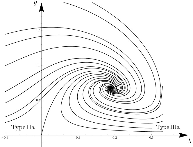
where the dots stand for the classical gauge fixing and ghost terms. The RG equations for the dimensionless Newton and cosmological constants, and , respectively, are well known [7], and their numerical solution [22] leads to the phase portrait in Figure 2.
On the half-plane with we can distinguish the trajectories of Type Ia, IIa, and IIIa, respectively, which are heading towards negative, vanishing, and positive values in the infrared, respectively. In the ultraviolet they emanate from the non-Gaussian fixed point (NGFP) which renders them asymptotically safe: .555 We refer the reader to [23, 24, 25, 26, 27, 28] for a partial list of recent results.
In the sequel we mostly focus on trajectories of the Type IIIa since
conceptually they give rise to the most interesting behavior, and
also because positive values of the cosmological constant are of special
interest phenomenologically.
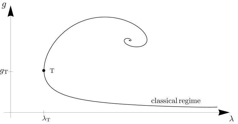
(2) The trajectories
of Type IIIa are special in that they possess a turning point
near the origin of
the -- plane. The -function of the dimensionless
cosmological constant vanishes there: .
Here denotes the scale at which the trajectory visits
the point , see Figure
2.
We are particularly interested in trajectories with
which pass very close to the Gaussian fixed point (GFP) located at
. They spend a long RG time in its vicinity and possess
an extended classical regime.
(3) While it is
straightforward to solve the RG equations numerically, there exists
a convenient analytical approximation for Type IIIa trajectories which
leads to transparent closed-form results often. It is obtained by
linearizing the RG equations666See eqs. (4.38) and (4.43) of ref. [7].
about the GFP. The linear equations are easily solved, and one finds
that the dimensionless couplings evolve according to
| (3.2) | |||||
| (3.3) |
The corresponding dimensionful quantities behave as
| (3.4) | |||||
| (3.5) |
The prefactor in (3.2) and (3.4) is a constant of order unity, which depends on the cutoff operator . For pure gravity it reads
| (3.6) |
where is one of the standard threshold functions defined in [7].
These solutions amount to a 2-parameter family of RG trajectories
whose members are labeled
by the constants of integration and , both
assumed positive. The linear approximation is valid within the classical
and the semiclassical regime of the trajectories. In the former, both
and are constant
essentially; in the latter, Newton’s constant still does not run appreciably,
while is proportional to . This behavior
is reminiscent of the cutoff dependence mentioned
in Section 1. As we shall see, their precise
interpretations differ, however.
(4) One easily
checks that the approximate Type IIIa trajectory (3.2)
and (3.3) indeed possesses
a turning point. Its coordinates are
| (3.7) |
and it is visited by the trajectory when assumes the value
| (3.8) |
Inserting (3.8) into (3.4) we observe that between and the cosmological constant increases by precisely a factor of two:
| (3.9) |
(5) Often it is advantageus to eliminate the original labels of the trajectories, , in favor of the pair :
| , | (3.10) |
The relabeling leads to
| (3.11) | |||||
| (3.12) |
Here is not independent but must be regarded a function of . The pertinent dimensionelss trajectory writes
| (3.13) | |||||
| (3.14) |
The representation (3.13) makes
it obvious that the function is invariant under
the “duality transformation” .
As a result, every given value in the
semiclassical regime is realized for two scales, namely and ,
respectively. (See ref. [29] for a detailed discussion.)
(6)
Once exceeds a certain critical value, , which is of
the order of the “Planck mass” ,
the linearization about the GFP is no longer a reliable approximation.
The (dimensionless) trajectory enters the scaling regime of the NGFP
then, and ultimately comes to a halt there: .
On the other hand, the dimensionful couplings keep running according
to the power laws
| (3.15) | |||||
| (3.16) |
when .
(7) Type IIIa trajectories
displays the following three independent length scales:
-
(i)
The Planck length as defined by the constant of integration ,
(3.17) -
(ii)
The turning point scale as determined by and ,
(3.18) -
(iii)
The Hubble-like length 777The name is motivated by the fact that equals exactly the Hubble length in the case of de Sitter space, and that .
(3.19)
In terms of those scales, the running cosmological constant along a Type IIIa trajectory may be characterised compactly by
| (3.20) |
with a transition scale .
Since , both hierarchies among these scales are controlled by the same dimensionless number, namely :
| , | (3.21) |
(8) With their parameters adjusted accordingly, the formulae (3.20) apply also to Einstein-Hilbert gravity coupled to a wide variety of matter systems [35, 36, 37, 38, 39], see [9, 40] for an overview.
When considering matter coupled to gravity in the following we focus on the subset of matter systems which possess Type IIIa-trajectories qualitatively similar to those of pure gravity, requiring that
| and | (3.22) |
The restrictions (3.22) assumed, the formulae (3.20) may be applied to pure and matter coupled gravity alike.
4 Self-consistent Background Geometries
In the previous sections we recalled how to define and compute the
Effective Average Action in a Background Independent setting. In this
section we assume instead that we already managed to compute a certain
RG trajectory , either via the path integral
or the FRGE. We introduce and analyze a number of scale dependent
objects (effective metrics, Laplacians, eigenvalues,
etc.) which “co-evolve” with , in the sense that,
(i), to compute at , the knowledge of
is sufficient, and (ii), the value of does not backreact
on the RG evolution .
(1) So from
now on the RG trajectory , interpreted as a curve
on theory space, is fixed once and for all. For the essential part
of our discussion it is not necessary that this trajectory
is a complete one that would in particular be UV-complete and
assign a non-singular function to any .
The perhaps somewhat surprising phenomena we are going to describe
are relevant even for incomplete trajectories of finite extension,
with , say. Those phenomena are most
pronounced in the semiclassical regime and, logically, they are unrelated
to all questions of non-perturbative renormalizability, whether by
Asymptotic Safety any other mechanism.
(2) Given
an RG trajectory
we can compute the background metrics that are self-consistent at
any point along this trajectory. Focusing on solutions with a vanishing
background value for the ghosts (), we must solve
the tadpole equation (2.9)
with .
In the sequel we assume that this has been done already, and has led
to a certain family of metrics .
So now we must learn how to interpret such explicitly scale dependent
background metrics.
(It is worthy to note that the self-consistent background metrics play also key role
in the computation of the entanglement entropy [30].)
4.1 From the “running” to the “rigid” picture
To prepare the stage, let us outline how one would extract physical
information from or more generally888In our general considerations we can easily include matter fields
into the discussion replacing everywhere.
Here stands for an arbitrary set of dynamical matter fields.
In fact, in the background field approach to quantum gravity,
is the prototype of a “matter-like” field. In the context of the
present paper, should be regarded logically detached
from , together with which it forms the full metric.
Issues of split-symmetry and its breaking [31, 32, 33, 34] will
play no role here,
, in order to confront its
predictions with with laboratory experiments or cosmological observations.
(1)
Let us expand the EAA in terms of a -independent set of basis
invariants, ,
and regard it as the generating functional of the running coupling
constants :999The overbar of indicates that we
are dealing with the dimensionful variant of the couplings.
| (4.1) |
Now, while it is certainly true that the physics of the (interacting, non-linear) gravitons is encoded to some extent in the -dependent couplings , that is only half of the battle. If the dynamically determined background geometry has a significant -dependence, the invariants , evaluated at the physical point , are a second and equally important source of scale dependence:
| (4.2) |
Let us assume that along the RG trajectory there exists an extended
range of -values where the metrics are
approximately flat and the running of is negligible,
giving rise to what we call a “classical regime”. For (notational)
simplicity we assume that this is the case at very low scales near
, but the following discussion applies equally well to any other
position of the classical interval on the trajectory.
(2)
Let us furthermore assume that the large classical Universe at low
scales is inhabited by physicists who are able to perform observations
and experiments both at those low classical scales, and at higher
scales where they perceive a non-trivial RG running already. They
might refer to the former observations as of “astrophysical” or
“cosmological” type, while the latter experiments concern the
“particle physics” of the - and -quanta.
How would these physicists exploit the action (4.2) when they try to match it against their observations? First of all they must take a decision about which metric they prefer to use when it comes to expressing the values of dimensionful quantities. Natural options include at the running scale , the metric related to the endpoint of the trajectory, or pertaining to any other, but once and for all fixed scale .
Since their macroscopic classical world is well described by , the physicists might consider it a sensible starting point to use also when they take first (experimental and theoretical) steps towards higher scales, with an appreciable RG running of the metric now. Doing so, it is natural to re-expand in terms of the set with the -argument of all invariants fixed to . This set contains the invariants needed to write down a background-dependent theory of gravitons and -particles propagating on a rigid classical spacetime.
Furthermore, one may try to discard the gravitons and use the sub-subset of invariants in order to formulate a “standard model of particle physics”. The metric of spacetime is not an issue then, it is a seemingly universal, external ingredient, typically the Minkowski metric or in the Euclidean formulation.
The re-expansion of the basis functionals (monomials) is of the form
| (4.3) |
with scale dependent coefficients . Inserting (4.3) into (4.2), we obtain a representation of the effective --theory in terms of -independent basis monomials:
| (4.4) |
The equations (4.2)
and (4.4) are two ways of writing
down the same functional. Therefore physicists analyzing their
measurements in terms of the rigid metric
rather than the scale-dependent one, , actually
do not directly measure the couplings, ,
the natural ones for doing FRGE computations, but the linear
combinations .
(3)
On top of this fairly simple re-organization of the EAA, there is
a second, much more subtle transformation which physicists using no
other metric but would want to apply to
. For them
it appears quite unnatural to parametrize the RG trajectory by the
variable , which is chosen such that is the cutoff in
the spectrum of . They will prefer using a new parameter,
, which is likewise connected to a cutoff, but now in the spectrum
of , the only Laplacian available
to the “-only” physicists.
This raises the nontrivial question of how is related to the familiar parameter which we routinely employ in our FRGE calculations. What makes this problem particularly intricate is that by evaluating at the operator itself acquires an explicit -dependence: .
Before we can address this problem and complete the resulting “rigid picture” of the RG evolution a number of preparatory steps is needed.
4.2 The Einstein-Hilbert case
Within the Einstein-Hilbert truncation the tadpole condition happens to have the structure of the classical Einstein equation:
| (4.5) |
The energy-momentum tensor
| (4.6) |
makes its appearence only if we generalize the Einstein-Hilbert truncation ansatz by adding a matter action .101010To make the truncation well defined, must not contain terms . In that case, (4.5) gets coupled to an additional matter field equation, .
Throughout this paper, we consider either pure gravity (), or matter-coupled gravity under the simplifying condition that, in the regime of interest, the -term on the RHS of (4.5) is negligible relative to the -term:
| (4.7) |
Here the assumption is that the role played by matter predominantly
consists in renormalizing the pure gravity couplings
and rather than introducing new ones. (An analogous assumption
is also implicit in Pauli’s reasoning.)
(1)
Thus it will suffice to solve equation (4.5),
for all of interest, with . Clearly this
is still a difficult task in general, but there is a simple way of
promoting any known classical solution (for a fixed cosmological constant)
to a family of -dependent metrics satisfying (4.5).
The identity ,
valid for any , implies that if is
a solution of Einstein’s classical equation with a fixed cosmological
constant , then
| (4.8) |
is a solution of its -dependent counterpart, eq. (4.5), for any with .
According to (4.8),
only the conformal factor of the metric really “runs” in this
class of scale dependent background geometries. Obviously the cosmological
constant determines the absolute scale of all lengths
computed from in the expected
way, but it does so differently for changing values of the RG parameter
.
(2)
Henceforth we employ the approximate analytic formulas for the Type
IIIa trajectory presented earlier. Furthermore, we identify
here, but other choices may be natural as well.111111For example, a hypothetical astronomer who is able to measure the
curvature of spacetime on a finite distance scale
would find it convenient to let . Then
| (4.9) |
where the ratio of cosmological constants,
| (4.10) |
is given by
| , | (4.11) |
and
| , | (4.12) |
for the semiclassical and the fixed point regime, respectively.
(3)
Background metrics of the rescaling type (4.8)
entail various simplifications:
- (i)
-
(ii)
The 4D tensor Laplacians associated with and , respectively, are related in a simple way,
(4.14) since
(4.15) and the Christoffel symbols, implicit in the Levi-Civita covariant derivative , agree for the two metrics.
4.3 Maximum symmetry: -type spaces
It will often be instructive to illustrate our general considerations by means of the technically simplest (Euclidean) background spacetime, the -sphere . Its radius is the only free parameter in the metric then, the corresponding line element being
| (4.16) |
where denotes the line element on the round unit sphere,
. The metric (4.16)
implies the Ricci tensor
and the curvature scalar .
(1)
The spectrum of the Laplacian on ,
acting upon fields of any spin, is well known [41, 42, 43, 44]. The
eigenvalues can be labelled by a single “quantum number”, ,
a positive integer, and one has
| , | (4.17) |
Here , , and are constants which depend on the spin, as well as on the dimension, in the general case.
For our present purposes it is sufficient to focus on eigenvalues with , leading to a universal formula:
| , | (4.18) |
This representation of the -eigenvalues is common
to all fields we shall encounter.
(2) Let us
suppose the sphere is a solution
to the Einstein-Hilbert tadpole equation (4.5)
at . This requires first of all, and a radius
. From eq. (4.9)
we then obtain immediately a family of scale-dependent self-consistent
metrics:
| (4.19) |
Clearly, at higher scales the spacetimes described by (4.19) are still spheres, but with a continually changing radius:
| (4.20) |
Typically is an increasing function of , causing the spacetime to shrink at high values of the cutoff scale.
5 The Spectral Flow
In Section 2 we discussed the bipartite spectra of for all -independent backgrounds in the domain of the functional . Knowledge of those spectra is necessary in order to compute the EAA. In this section we shall consider a number of related, but inequivalent spectrum-derived objects in order to analyze and interpret an already known trajectory .
5.1 Spectral flow induced by the RG trajectory
To compute we had to solve the eigenvalue problem (2.10) for all possible background metrics, at least in principle. Assuming now that we have the explicit EAA in our hands and try to extract its physics contents, we are led to go “on-shell”, i.e., to evaluate and its functional derivatives at .
Therefore our next task is to understand the meaning of the eigenvalue equation (2.10) under these special circumstances, and to determine the, by now dynamically selected, space of the effective degrees of freedom, .
The following algorithm makes it precise what it means to “insert” into the UV/IR decomposition (2.11). In fact, at first it might appear somewhat confusing that there is a second source of -dependence now, over and above the -condition .
-
(i)
At every fixed scale we freeze the -argument in , and as a consequence also in the eigenvalue equation (2.10). This simplifies matters since rather than considering all possible backgrounds we can now restrict our attention to a single point in the space of background metrics, namely .
-
(ii)
And yet, the overall situation is more involved now since this single point changes continually when we move along the RG trajectory from one scale to another. It traces our a certain curve in the space of metrics: .
-
(iii)
The curve of metrics generates an associated curve in the space of Laplace operators, . Each one of those Laplacians, , gives rise to its own eigenvalue problem:
(5.1) At least in principle we can solve (5.1), for one value of after another, and thus obtain a “curve of spectra”, or a spectral flow, . At the same time we find the associated eigenbases, .
-
(iv)
Next we determine the respective cutoff modes implied by all spectra that occur along the curve. At a given point on the curve, having the paramter value , say, we require that,121212In the case of a discrete spectrum we relax this condition as before: The cutoff mode possesses the smallest eigenvalue equal to, or above .
(5.2) and we solve this condition for . In this manner we obtain the label which identifies the cutoff mode pertaining to the spectrum of the background Laplacian (on-shell!) at that specific point of theory space which is visited by the RG trajectory when .
-
(v)
Finally we distribute the modes of the eigenbasis over two sets, putting those with with eigenvalues
and into the sets and , respectively.
Repeating this algorithm for all , we obtain the cutoff mode for any point of the trajectory, , or more explicitly . Likewise we get the corresponding “curve” of UV- and IR- subspaces, .
In this way we have constructed the decomposition of the eigenbases,
| (5.3) |
which replaces (2.11) when “going on-shell” and brings in its own -dependence.
Let us now be more explicit and specialize for solutions to the tadpole equation of the rescaling type (4.9).
5.2 Spectral flow for rescaling-type running metrics
If the -dependence of resides in a position-independent conformal factor only, , the eigenvalue equation (5.1) of is solved easily for all provided its solution is known at a fixed , say .
Let us imagine we managed to solve (5.1) in the special case of , and we know all eigenvalues and eigenfunctions :
| (5.4) |
Multiplying eq. (5.4) by , and exploiting that by (4.14), we obtain
| (5.5) |
Comparing this relation with eq. (5.1) we conclude that, for rescaling-type metrics, the mode functions are actually independent of , while their eigenvalues possess a simple scale dependence given by :
| (5.6a) | ||||
| (5.6b) | ||||
5.3 Interpretation of the spectral flow
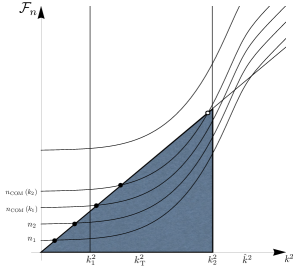
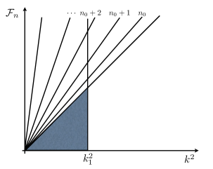
In Figure 3 we sketch schematically
a generic spectral flow stemming from a typical RG trajectory
along which is a rapidly increasing
function of . The horizontal axis corresponds to the trajectory’s
curve parameter , while the two vertical lines represent two specific
values of this parameter, and , respectively.
The presentation in Figure 3 is analogous
to Figure 1, whereby
replaces the constant eigenvalues . The -dependence
of the entire spectrum
is what we refer to as the spectral flow induced by the RG evolution
of the background metric.
(1) Note that the
scale dependence experienced by the eigenvalues when we move along
the trajectory, per se, has nothing to do yet with the concept
of cutoff modes.
In order to determine the cutoff mode for a certain scale, say , we first locate the points in Figure 3 where the graphs of all intersect the vertical line at . Then we check whether the points of intersection lie above or below the diagonal (). The UV/IR discrimination is achieved then by sorting all modes with eigenvalues intersecting, or precisely on the diagonal into the set , and those which intersect below the diagonal into .
The cutoff mode, by definition, is the one with the smallest eigenvalue among the modes in . As indicated in Figure 3, the cutoff mode pertaining to the specific scale carries the label .
Clearly, the specific mode with the label ,
fixed, like all the modes, has an eigenvalue
that depends on the point in the theory space the RG trajectory is
currently visiting, i.e., it depends on in its role as a curve
parameter. However, for parameter values the mode with
has no special meaning in general.
(2)
As we know, are the modes
not yet integrated out at , and they consitute the degrees
of freedom governed by the effective action .
In Figure 3 they are represented by
the eigenvalues passing through the part of the shaded triangle that
lies to the left of the vertical -line. Exactly as in Figure
1 for the constant , below all those
eigenvalues intersect the diagonal only once; in Figure 3
the corresponding intersections points are marked by black circles.
The physical interpretation of this behavior is deceptively simple:
When we lower so that the vertical -line sweeps
over one of the black dots on the diagonal, one more mode is relocated
from into .
And, naively, one might think this is exactly as it always must be
since lower cutoffs amount to more modes being “integrated out”.
(3)
However, the situation changes profoundly when we move to higher scales,
, in Figure 3, say. If the
cosmological constant and increase
sufficiently rapidly with , it can happen that below the graph of
one and the same eigenvalue intersects
the diagonal more than once. Indeed, Figure 3
is inspired by the spectral flow along a Type IIIa trajectory where
this behavior arises as a consequence of the very strong -running
in the semiclassical regime, see below.
Figure 3 displays eigenvalues which both enter and exit the shaded triangle to the left of the -line; the intersection points with the diagonal are marked by black and open circles, respectively. When we lower it may happen that the vertical -line sweeps over one of the open circles. Again this means that a certain mode changed its UV/IR status, but this time the relocation is from to !
At first sight this seems to be a rather strange and perhaps “unphysical”
phenomenon. After all, we expect that lowering the cutoff leads to
integrating out further modes, and this would move them from
into . Here instead the opposite happens, and
a mode classified “UV” all of a sudden becomes “IR” by lowering
the scale.
(4) This apparent paradox gets resolved,
though, if we recall that the standard equivalence
holds for the functional
with -independent (off-shell) field arguments. Importantly, during
the computation of the EAA this equivalence still holds true, also
in the present case. The actual cause of the unexpected spectral behavior
is that when we take the fields on-shell and choose the self-consistent
background they, unavoidably, acquire an extra -dependence which
entails a non-trivial spectral flow then.
A transition caused by a lowered -value is by no means “unphysical” therefore. On the contrary, it points to the physically important fact, that the effective theory given by has gained a new degree of freedom it must deal with; its quantum or statistical fluctuations are not yet included in the renormalized values of the couplings comprised by .
As Figure 3 illustrates, at a sufficiently low scale the new IR-mode crosses the diagonal a second time, thus leaving the triangle that encompasses the current IR modes.
5.4 Special cases: Type IIIa and
To make the discussion more explicit at this point, we specialize
for Type IIIa trajectories and the maximally symmetric solutions
to the Euclidean Einstein equation.
(a) For
a trajectory of Type IIIa all qualitatively essential features are
encapsulated in the simple approximate formulae (4.11)
and (4.12) for the semiclassical and the
fixed point regime, respectively. Inserting them into (5.6b)
we obtain
| (5.7) |
The scale dependence of these eigenvalues gives rise to a spectral
flow with exactly the features depicted in Figure 3.
The RG effects are strongest in the semiclassical regime. There
increases very rapidly with , and this does indeed lead to eigenvalues
which intersect the diagonal twice.
(b) Opting
for the -type solutions of the tadpole equation, the generic
label amounts to a single integer, and we get from equation (4.18),
for ,
| (5.8) |
In particular in the semiclassical regime, the -dependent radius of the sphere, , decreases rapidly for increasing , thus causing a corresponding growth of the eigenvalues:
| (5.9) |
In the fixed point regime, where
| (5.10) |
the self-consistent value of the radius decreases more slowly with . Note also that in the analogous Lorentzian setting corresponds to the inverse Hubble parameter, i.e., the Hubble length.
6 The new RG parameter
Now we are prepared to return to the physicists living at , who would like to reformulate the entire effective theory (4.4) in terms of . As we mentioned already, this involves reparametrizing the (fixed!) RG trajectory that is under scrutiny, , in terms of a new scale parameter .
6.1 Introducing as a cutoff scale
Ideally, in analogy with which is a cutoff in the spectrum of , the new parameter should be an eigenvalue cutoff for the operator . The latter has no scale dependence, and it is the only Laplacian the “-only” physicists want to use.131313Again we emphasize that here we are analyzing a given RG trajectory, rather than computing it. We are not proposing any different off-shell functional here. In particular the - and the -schemes, respectively, are not different ways of expanding the integration variable under the path integral. In fact, in the process of computing the functional , those two cases are completely indistinguishable, as we neither set nor at that stage; we rather keep fully arbitrary, but independent of any scale.
In principle, the division of the eigenfunctions in UV-modes and IR-modes, respectively, can be described without recourse to any metric, namely by characterzing the cutoff mode and the sets directly in terms of the mode labels . Usually is chosen to be a dimensionless multi-index (one or several “quantum numbers”) that is not linked to any particular metric.
Considering running metrics of the rescaling type, equation (5.6a) tells us that the eigenfunctions have no explicit scale dependence despite the running of the metric. Therefore, if a certain function is the cutoff mode at , it is so also at any other point along the curve of spectra induced by the running background. This is true regardless of whether we parametrize the curve by the standard parameter or by the new variable . The difference between the - and -scheme, respectively, arises only when we convert the label to the (dimensionful) square of a covariant momentum.
By considering eq. (5.6b) at we obtain
| (6.1) |
In the -scheme, the quantum number is converted to a momentum, , by setting
| (6.2) |
and solving for . Now we convert the same quantum number to the momentum preferred by the “-physicists”. In complete analogy with (6.2) they set
| (6.3) |
Recall that and denote the, in general different, eigenvalues of and , respectively, belonging to their common eigenfunction . If we now insert (6.2) and (6.3) into (6.1) we obtain
| (6.4) |
Solving for yields the new RG parameter as a function of the old one:
| (6.5) |
This simple, yet fully explicit formula will be a crucial tool in the following. In fact, there are two immediate applications in which the function and its inverse play a prominent role, as we discuss next.
6.2 Completing the rigid picture:
Let us assume for a moment that it is possible to invert the relation (6.5) and obtain as a function of , i.e., . Under this assumption we can finally complete our task of recasting the EAA from (4.4) in a style which eliminates everywhere in favour of . This is achieved by setting
| (6.6) |
This variant of the EAA refers the physics of all “particles”, the graviton included, to one metric only, namely the one that is self-consistent at .
6.3 Cutoff modes: relating to
In order to determine the cutoff modes along the spectral flow, i.e., the -dependent “quantum number” , we need information about, first, the RG trajectory, and, second, about the structure of spacetime. The former information is encoded in the relationship and its inverse, while the latter is provided by the (single) spectrum of the scale independent Laplacian . Given these data, eq. (6.3) yields the condition
| (6.7) |
which is to be solved for then.
For instance, in the case of the spacetime, the relevant spectrum reads , and so
| (6.8) |
It is assumed here that , so that is a quasi-continuous variable and we can be cavalier as for its integer character.
Note also that since and , the result (6.8) is equivalent to
| (6.9) |
This formula nicely illustrates how the two natural perspectives on the RG flow are connected, namely the conventional “running picture” which employs the scale parameter leading to a running spacetime metric, and the new “rigid picture” based on the scale together with the rigid metric . In the example, the correspondence ( and ) allows us to interpret one and the same mode, labelled , as either , or as , respectively, depending on whether the “rigid” or the “running” perspective is adopted.
7 The Global Relation Between and
7.1 Non-invertibility of
Along the RG trajectory of the Type IIIa, the ratio of the cosmological constants, , is well approximated by (4.11) and (4.12). This turns eq. (6.5) into
| (7.1) | |||||
| (7.2) |
A plot of the function is shown in Figure 4.
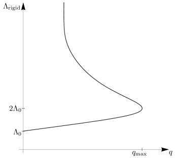
Let us follow a Type IIIa trajectory from the IR towards the UV, see Figure 2b. At all scales far below the turning point, , it is in the classical regime, quantum effects are negligible, and approximately. Then, at the trajectory passes the turning point, the -running of the cosmological constant sets in, and once , eq. (7.1) yields roughly
| (7.3) |
This behavior is rather striking: An increasing value of the standard RG parameter implies a decrease of the newly introduced scale . In fact, the function has a maximum precisely at the trajectory’s turning point, , where it assumes the value
| (7.4) |
For all the other points in the semiclassical regime, eq. (7.1) always associates two -values to a given , see Figure 4.
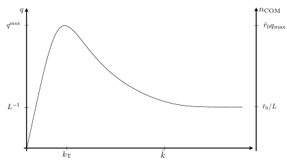
Obviously the function is not monotonic, and eq. (7.1) cannot be inverted in the entire domain of interst. Therefore, globally speaking, the map is not an acceptable reparametrization of the RG trajectory ; it fails to establish a diffeomorphism on the RG-time axis.
Nevertheless, locally, namely for either or , eq. (7.1) can be inverted, yielding the following two branches of for :
| (7.5) |
For given, the functions and return values smaller and larger than , respectively. They are joined at .
If we follow the Type IIIa trajectory beyond we enter the asymptotic fixed point regime. The cosmological constant scales as there, hence , and as a consequence, becomes perfectly independent of asymptotically:
| (7.6) |
Note that since , the length parameter is essentialy the radius of the Universe (Euclidean Hubble length) according to the -metric. Hence the asymptotic value is an extremely tiny momentum square, even by the standards of the -physicists employing the rigid metric. For them, the Universe is a sphere of radius , and is of the same order of magnitude as the lowest lying eigenvalues in (4.17) for the normal modes on this sphere.
In the present paper, the Asymptotic Safety based ultraviolet completion of Quantum Einstein Gravity plays no important role. We focus here on the implications of the “strange” relationship between the two alternative RG scales and which we summarize in Figure 4. Its salient properties are entirely due to the -running in the semiclassical regime. In the following we restrict the discussion to this regime mostly.
7.2 Scale horizon and the failure of the rigid picture
By the very construction of the FRGE, the IR cutoff scale provides a globally valid parametrization of the RG trajectories, . We tried to introduce a new RG-time parameter such that the size of all (dimensionful) eigenvalues is expressed relative to the rigid metric rather than the running one, . Now we see this “rigid metric”-persepective on the RG flow is doomed to fail.
This perspective appears to be the natural one for the -physicists,
who are either ignorant of the RG running in the gravitational sector,
or try to incorporate the quantum gravity effects into the couplings
of an effective action which, however, is still conservative in relying
on fields that live on the same classical spacetime at all RG times.
(1)
As the function cannot be inverted globally on
the RG-time axis, it is clear that the reparametrized action
of eq. (6.6) can make sense at best locally.
For example, it does yield a consistent description for small momenta
, for which the “minus” branch
of (7.5), ,
establishes a one-to-one relation between and . In a way,
since here, this amounts to the “perturbative”
branch of .
However, starting out at and then following the Type IIIa trajectory
from the IR towards the UV, we come to a point where the -parametrization
breaks down, namely . This
value is equivalent to , i.e., precisely when the
trajectory passes through its turning point, the -description
becomes untenable: Moving from the turning point further towards the
UV,141414Or in unambiguous, global terms: “Increasing from
to with , … .” while still adhering to the parameter , it would have to decrease
rather than increase, thus conveying the utterly false impression
of an RG evolution which runs in the wrong direction.
(2)
We conclude that the trajectory’s turning point acts as a kind of
horizon for the -physicist who try to ignore the RG evolution
of the spacetime geometry as long as possible. The rigid metric perspective
on the Background Independent RG flow comes at the price of a “scale horizon”
on the RG time axis (rather than spacetime) beyond which
strong quantum effects render it inconsistent.
Remarkably enough, this scale horizon has nothing to do with “exotic”
Planck mass physics. Rather it occurs where the semiclassical -running
of the cosmological constant becomes appreciable, namely at the much
lower turning point scale . Recall that if we were to
model real Nature by a Type IIIa trajectory, we find a turning
point scale as low as , see
[h3].
(3)
Figure 5 illustrates the role
played by the horizon in connection with the cosmological constant
(problem). The reparametrized action of eq. (6.6)
includes a cosmological constant term ,
and the -physicists regard
as their natural scale dependent cosmological constant. Combining
eqs. (4.10) and (6.5)
it is given by ,
and with (7.5) we obtain
the double-valued relation
| (7.7) |
This relation is depicted in Figure 5, with the plus (minus) sign corresponding to the upper (lower) branch of the diagram.
The -physicists have no logical difficulties interpreting the lower branch of . They are unable, however, to pass around the horizon at , if they insist on using the scale . Seen as a curve parameter which parametrizes the RG trajectory, is a “good” coordinate on the RG time axis only below the turning point. In order to go beyond the horizon a “better” coordinate is needed, such as for example, which is acceptable even globally. This hints at a certain analogy between the scale horizon and the familiar coordinate horizons in spacetime.
On a more positive note we may conclude that nevertheless the rigid picture based upon the perturbative, i.e., the -branch is applicable and equivalent to the running picture provided no relevant momenta exceed .
7.3 The boundedness of and
While the scale is not a fully satisfactory alternative to
as a RG time, the function has another important,
and logically independent application, namely the determination of
the cutoff modes along the flow. This application does not
require the inverse function.
(1) In Subsection
6.3 we showed that
is determined by eq. (6.7), which requires
as the essential input. Specializing for -spacetimes,
eq. (6.8) yields ,
which is valid in the approximation of a quasi-continuous spectrum
employed throughout. Thus, the -quantum
number of the cutoff mode is known as an explicit function of :
| (7.8) |
The scale dependent implies a corresponding decomposition of all normal modes: modes with quantum numbers belong to , all others to .
Since, for spheres, differs from by a constant factor only, Figure 4 can also be regarded as a representation of in dependence on the global RG parameter . Therefore we conclude that assumes a maximum at the turning point:
| (7.9) |
The integer is bounded above and never becomes very large: nowhere along the Type IIIa trajectory, evaluated “on-shell” with a self-consistent background, a cutoff quantum number occurs that would exceed the turning point value.
It must be stressed that this result151515Note that the impossibility of using as an alternative flow parameter
is irrelevant here. is perfectly well-defined, conceptually meaningful, and in fact related
to a dynamical mechanism that is easily understood in general physical
terms, as we shall discuss below.
(2) According
to Figure 4, there can exist pairs of scales,
and , smaller and larger than , respectively,
giving rise to the same quantum number .
This proves, within the Einstein-Hilbert truncation, that the spectral
flow sketched schematically in Figure 3
is indeed qualitatively correct.
We mentioned already the possibility that certain eigenvalues intersect the diagonal twice. At one scale they change their UV/IR-status in the IRUV direction, while they move in the opposite direction UVIR at another scale (indicated in Figure 3 by the black and open circles, respectively.)
Consistent with that, the plot in Figure 4 reveals that decreases, implying that the set looses modes, when is increased further above . Actually this is the same phenomenon which is also visible in Figure 3, albeit in a different way: The cutoff mode for is identified by that particular eigenvalue which lies on, or just barely above the diagonal at . Now, given that grows very rapidly with , basically all eigenvalues will eventually exceed when we let . Hence looses more and more modes when , and so decreases correspondingly.
The occurrence of this phenomenon is now fully confirmed by the explicit Einstein-Hilbert result plotted in Figure 4, where does indeed decrease to a very small value. It is determined by the fixed point properties ultimately.161616The approximation of the quasi-continuous spectrum may become invalid then.
It should be clear now that this unfamiliar behavior is by no means
in conflict with the usual rule “integrating out modes, i.e., making
smaller, requires to be lowered.” This
rule applies to the calculation of the
for -independent off-shell arguments. Here instead we go on-shell
and follow the physical metrics along the
RG trajectory.
(3) The unexpected behavior
of , in particular its boundedness,
is one of our main results. For this reason let us emphasize that
the underlying mechanism is easily understood in elementary physical
terms and should be regarded particularly robust therefore.
The eigenvalues being of the form , we can make them larger in either of two ways, namely by increasing , or by decreasing the radius of the sphere. The first way is the one we are familiar with from the off-shell EAA, leading to the standard connection, .
The second way, decreasing the radius, becomes an option only when the background geometry is taken on-shell. But then it may happen that a certain increment of is “used up” predominantly to make the radius smaller, rather than to go to a higher quantum number. What Figure 4 tells us is simply that, when , the shrinking of the spacetime radius with growing is so strong that we even can afford lowering and nevertheless get a bigger .
Thus it is also clear that the basic mechanism is not restricted to spheres (having ). All that is required is a self-consistent geometry and a range of scales such that .
7.4 Spectral flow in a scaling regime
In this paper we are mostly interested in the semiclassical regime and in properties that are largely insensitive to the RG behavior at . Let us nevertheless digress for a moment and assume that the RG trajectory is asymptotically safe and hits a non-Gaussian fixed point when . In its vicinity, , and so all the eigenvalues behave as , see Figure 6. Remarkably, no eigenvalues cross the -line in this regime, and is the empty set.
Figure 6 can be seen as the continuation for of the flow in Figure 3 or, in its own right, as the flow of the undeformed fixed point theory for all .
8 Application to the Cosmological Constant Problem
Finally let us critically reconsider the standard argument concerning the alleged unnaturalness of a small , which we reviewed in the Introduction. As we shall see, this argument about the gravitational effect of vacuum fluactuations is flawed by not giving due credit to Background Independence. Instead, by doing so we can show that the domain of validity of this calculation is considerably smaller than expected, and that it has actually nothing to say about a potentially large renormalization of .
8.1 Preliminaries and assumptions
(1) The thought experiment. Implicit in the reasoning of Subsection 1.1 is the imaginary removal of a selected quantum field, say, from the set of all fields that exist in Nature, and the assumption that the remaining fields jointly give rise to essentially the Universe as we know it. One then gradually “turns on” the quantum effects of in this pre-exisiting Universe, and wonders about the backreaction the extra field exerts on it.
The tacit assumption is that the backreaction is weak so that the Universe has a chance to look like ours even with the extra field fully quantized, but this then turns out not to be the case according to the standard analysis. In our opinion this should first of all raise a number of questions and concerns about the very setting of this thought experiment, over and above the physics issues it tries to address. For example, should the Universe before or after adding be as large as ours? In the latter case, the Universe without is strongly curved, so, why should the calculation of in flat spacetime be sufficient? Under what circumstances does the quantum Universe, with and without , actually appear to be semiclassical?
To fully avoid difficulties and conceptual problems of this kind we replace the original thought experiment by a logically simpler and more clear-cut question for theory. While aiming at the same phyics issue, it avoids the dubious separation of a special field from the rest of the Universe, and it also does not rely on the possibility of treating one part of the Universe as classical, while the other is quantum mechanical.
The question is as follows: In a fully quantum Universe with
all fields quantized, what is the shift of the cosmological constant,
, that -observers ascribe to the zero-point
energies of all quantum fields together? Within the EAA approach
to quantum gravity, it will be possible to answer this question in
an unambiguous way, purely by inspection of the trajectory,
, and the trajectories derived from it, .
(2) Scope and assumptions. Let us set up the
EAA framework now and outline its range of validity. The quantum fields
in questions are and a collection of matter fieds ,
their dynamics being ruled by a given solution to the flow equation,
. The argument we are going
to present is based upon the following assumptions then:
(i)
We assume that, in the --sector, the RG trajectory
is qualitatively equivalent to a Type IIIa trajectory of the Einstein-Hilbert
truncation. Its - projection looks as in Figure 2b.
More precisely, it is sufficient that it does so for .
While the existence of a turning point
is of essential importance, our argument does not require a specific
behavior, such as the approach of a fixed point,
for example. Referring back to Section 3
it is clear that the requirement of a turning point is met under very
general circumstances. All one needs is a semiclassical regime where
behaves as in eq. (3.4),
i.e., , whereby
and .
(ii) Furthermore, we assume that
, i.e., ,
as in real Nature. This condition is even weaker than in the standard
calculation: The latter sums up the zero-point energies of a field
in flat space and so corresponds to letting .
By (3.21) the condition
implies a clear separation of scales: .
Another consequence is that ,
which allows for the technically convenient approximation of a quasi-continuous
spectrum at the scales of interest.
(iii) No
real matter particles are included. Virtual particles are taken into
account by the influence they have on the RG running of and
. The -term in the tadpole equation
(4.5) is assumed negligible.
(iv)
The solutions to the tadpole equation which we consider are ,
or de Sitter metrics of the rescaling-type (4.9).
Because of the highly symmetric spacetime, the immediate applicability of our discussion will be restricted to cosmology basically. Furthermore, since the cosmological constant term in Einstein’s equation must dominate over , its natural domain of applications includes a vacuum dominated era of late-time acceleration such as the one we presumably live in. Luckily, this is anyhow the regime where the cosmological constant is observationally accessible to us.
The reader must be warned that, when interpreting our results, it is important to keep the above limitations in mind and to refrain from transferring the results to more complex physical problems involving matter at a significant level, and/or less symmetric geometries with several relevant scales.
When the stress-energy tensor in Einstein’s equation is more important than the -term, and is -independent in the regime of interest, the new on-shell effects resulting from a running metric will disappear immediately.
Moreover, in multi-scale
problems a straightforward tree-level evaluation of the EAA is insufficient
in most cases. In particular, we do not expect that typical laboratory-scale
scattering experiments are in any way affected by those effects
since the standard model interactions are overwhelmingly strong at
the corresponding energies.
(3) What will (not) be shown.
It is to be stressed that we do not claim, or try to prove,
that the solutions to the RG equations necessarily yield values of
which are always small, thus explaining why Nature
could not but choose the exeedingly tiny number .
Rather, we show that if the Universe is described by a trajectory having , then -physicists can rightfully attribute an energy density to the quantum vacuum fluctuations which is at most of the same order as the -contribution. Clearly, this result is quite different from the usual one, and importantly, it cannot nurture any ideas about a small being “unnatural” in presence of quantum fields.
8.2 No naturalness problem due to vacuum fluctuations
Let us go through the various steps of the EAA-based reasoning now.
(1) The input.
Starting out from the given RG trajectory, ,
we construct the associated trajectories in the spaces of metrics,
, and of Laplacians, .
The spectral flow of the latter then attaches well-defined sets
to all points along the trajectory.
(2) One spectral flow only.
In general the cutoff modes and
would depend on the tensor type of the field
acts upon. In the case at hand we are entitled to ignore this dependence.
We are interested in the quasi-continuous part of the spectrum (quantum
numbers ) where the eigenvalues are independent of the tensor
rank, cf. Subsection 4.3. (Their degeneracies
are not, but they play no role.)171717Analogous remarks apply to fermions. For Dirac fields one may employ
the squared Dirac operator in place of the Laplacian. The two operators
differ by a non-minimal (curvature) term which, again, is inessential
for not too low eigenvalues.
(3) Read off rather than invent: the degrees of freedom.
At every fixed scale ,
is comprised of those modes that are not “integrated out” at the
point on the trajectory, i.e., their quantum fluctuations
are not yet accounted for by renormalized values of the coupling constants
in the EAA.
This allows us to conclude that
can be regarded the precise description, and translation to the EAA
framework, of the degrees of freedom whose zero point energies are
summed up by the standard calculation in the Introduction. The modes
constitute a classical field
theory for which , similar to before, plays the role
of an ultraviolet cutoff, and has a status analogous
to a bare action specified at this scale.
(4) The rigid picture comes into play.
To complete the reinterpretation of the traditional -computation
in the Background Independent setting we observe that this computation
must be ascribed to -physicists as it employs the
rigid and (almost) flat metric
to a maximum extent. The dispersion relation
and the cutoff , for instance,
involve the flat metric. Hence, on the EAA-side, it is the “rigid”
picture of the RG flow that must be used in a comparison of the standard
and the Background Independent approach. Therefore we re-express the
EAA at this stage in the form of the new action introduced
in Subsections 4.1 and 6.2.
(5) What the EAA tells us about .
Now we pose the question: Assume a team of -physicists have
measured the cosmological constant of their Universe, ,
and they are in possession of the untruncated EAA functional.
They employ it in order to deduce the contribution to the cosmological
constant, , that originates from the zero point oscillations
of all quantum fields. What order of magnitude will they find for
the ratio ?
The answer proceeds as follows: No matter what value of we pick, is always a comparatively “small” subset of all the field modes, its elements having -eigenvalues that are bounded above and “quantum numbers” . The function , sketched in Figure 4, has a maximum at . Thus we conclude, on the basis of the actual RG evolution, that the largest possible set of not-yet-quantized degrees of freedom, , occurs in the effective field theory belonging to the turning point, the hallmark of a Type IIIa trajectory.
Let us now fix some scale and read off the true contribution which, upon quantization, the modes in will supply to the cosmological constant. We perform the quantization within the EAA framework where it amounts to RG-evolving the “bare” action down to the effective action by following the prescribed trajectory. One of the running couplings involved is the total cosmological constant, and it evolves from to . As a result, is the shift due to the quantization of the modes in . For the simplified trajectory in eq. (3.4) we obtain
| (8.1) |
At this point it becomes crucial to carefully distinguish the “running”
and the “rigid” pictures of the RG evolution.
(a) Running picture.
The running picture employs as the independent
evolution parameter. Therefore it is meaningful to consider
and the corresponding shift for any ,
so that, by (8.1),
can become arbitrarily large when is a scale sufficiently
high. The physics interpretation of this large will
be given in subsection 8.4.
(b) Rigid picture.
Below the turning point, the description of the RG evolution in terms
of , involving ,
with , is equivalent to the running
picture. As we know, the function
assumes a maximum at , and is bounded above,
,
cf. Figure 4. Inverting it locally, one
obtains two branches, , with ,
cf. (7.5), but we use only
the perturbative “minus”-branch on which .
In order to determine , the “-physicists” adhering to the rigid picture must first of all fix a certain momentum, , in such a way that this is actually realized as a parameter value that specifies a point on the RG trajectory given. This implies that a scale must be chosen, since no value of the global RG parameter will ever result in a scale .
Given , there exists a well defined set of not-yet-quantized modes , and we ask about the shift caused by the inclusion of their fluctuations. On the perturbative branch, amounts to , and so with defined as in Subsection 7.2. The explicit function was given in eq. (7.7), and Figure 5 shows a plot of it.
Along the perturbative branch, the lower one in Figure 5, grows monotonically by a factor of when the -physicist increase the scale from to , changing from to . The shift is maximum when , yielding , and so
| (8.2) |
This, finally, is the answer to the question we posed above: Within the rigid picture, when applicable, the shift of the cosmological constant due to the vacuum fluctuations will always be at most of the order of magnitude of the IR value .
This completes the proof of the assertion made above.
(6) To be, or not to be applicable.
The above answer subsumes two logical possibilities:
(i)
The rigid picture is applicable and implies .
This requires all , in particular the UV cutoff for ,
to be not greater than . So, since is equivalent
to the cutoff from the Introduction, .
(ii)
The rigid picture is not applicable as we compute the
for modes with beyond
the scale horizon: .
In this case, can be large, but
the effective theories for and , respectively, are
no longer continuously connected by a RG trajectory
whereby is the proper-momentum of a scale independent metric
. They lie on opposite sides of a “scale
horizon”.
In the following subsections we discuss the two cases in turn.
8.3 Validity of the standard calculation
Now we are able to pinpoint what precisely is wrong about the standard arguments concluding that huge values of summed-up zero point energies render a small unnatural. In the present notation the integral (1.1) reads
| (8.3) |
We switched to the notation for the momentum since it is “proper” with respect to a scale independent (almost flat) metric, , and the same metric underlies the kinetic term of the massless free field that is being quantized.
Let us now estimate the domain of applicability of (8.3) by trying to identify it with a sub-sector of a Background Independent EAA analysis based on a trajectory describing an approximately free massless field at low scales, the graviton being the prime example.
At least in principle, the classical -theory, once identified by means of the EAA, can also be quantized by any other, that is, non-FRG method. In this spirit, (8.3) can be seen as an alternative, albeit approximate way of recovering the cosmological constant’s leading RG running, provided one identifies the UV cutoff with the floating RG scale. Concretely, ascribing (8.3) to the rigid picture, we must identify , as indicated in (8.3).
However, when it comes to interpreting the role of the -dependence
in (8.3), the Background
Independent approach (EAA) and the standard one (QFT in classical
curved spacetime) differ in a significant way.
(8a) Standard approach:
In traditional QFT on a fixed spacetime, one starts by making the
divergent integral finite in an arbitrary way which needs not to have
a physical interpretation, here by a momentum cutoff, then one adds
to a -dependent
counterterm such that
approaches the observed cosmological constant
for , and only when this limit is taken,
once and only once, one computes a metric, solving Einstein’s equation
with the parameter inserted.181818Clearly, this rough description can be refined or modified in many
ways; they would not affect the main conclusion though. Hereby, the adjustment of
involves the notorious fine-tuning which is behind the naturalness
aspect of the cosmological constant problem.
Note that, in the standard setting, the only point of contact between the QFT calculation and the curvature of spacetime is the single quantity . In the language of perturbative renormalization theory, it is one of the “renormalized” or “physical” parameters which appear in the conventional effective action , with the UV cutoff removed, and in absence of any IR cutoff. While this allows us to identify with from the EAA side, , it also points towards the following potential insufficiency of the standard treatment which we have not mentioned yet:
Whatever the vacuum fluctuation is like, no matter how violent it
is, or whether it has a Planck- or a Hubble- size wavelength, it
can impact the geometry of spacetime only via the eye of a needle,
namely the renormalized cosmological constant, . In
Einstein’s equation it multiplies the no-derivative term and controls
the properties of solutions at the largest possible length scales.
But is it really plausible to assume that, say, micrometer-scale fluctuations
influence the spacetime geometry predominantly on cosmological
scales? Why should cause and effect be separated by 30 orders of magnitude?
We shall come back to this particular aspect of the problem in Subsection
8.4.
(8b) EAA approach:
There are two relevant characteristics. First, the Background Independence
of the setting allows the dynamics to determine the background metric,
and second, every quantum field theory is regarded as the limit
of a sequence of effective field theories. The combination of both
properties implies that, unavoidably, dynamically selected backgrounds
are scale dependent. According to the effective field theory interpretation
of and , the integral (8.3)
describes how the cosmological constant, and via (4.5)
the curvature of spacetime, depend on the momentum of the probe
that is used to explore the structure of the Universe. The full quantum
theory is obtained by letting .
By comparing (8a) and (8b) it becomes evident that, for no Type IIIa trajectory whatsoever, the standard background dependent calculation can be equivalent to, or a meaningful approximation of the Background Independent EAA-based one.
In the standard approach, the limit of the integral (8.3) should be taken, while the EAA requires . The problem here is not that the limits are different, and that the limit does not exist in the former case: After all we are prepared to admit a counterterm. What is fatal for the standard approach is rather that the entire flat space-based calculation leading to (8.3) breaks down already at a scale much lower than , namely . From there on the rigid picture cannot be mantained any longer. It is then advisable to switch to the running picture by means of the which the horizon can be crossed without problems.
As long as the calculation is valid, the summed zero point energies given by (8.3) never exceed , and is at most . So we see that
| (8.4) |
which is essentially the same as (8.2).
Thus, again, we conclude that the summation of zero point energies in flat space cannot be used in order to claim that a small cosmological constant is “unnatural”.
8.4 Where has the large spacetime curvature gone?
Above, in (5) and (6) of Subsection 8.3, we mentioned that when one crosses the scale horizon and explores scales , now relying on the running picture, the induced cosmological constant can become arbitrarily large. In the semiclassical regime, for example, .
Now, this appears to be a resurrection of the notorious standard result with its disastrous consequence that the natural size (Hubble length) of the Universe should be of the order of a Planck length. This interpretation is false, however:
By going through the steps of the EAA-based analysis we have learned that, for a physical interpretation of the unbounded growth of above the turning point, it is compulsory to equip spacetime with a running self-consistent metric, . This metric entails a scale dependent curvature then,
| (8.5) |
and according to the effective field theory interpretation, this curvature is observed in experiments which scan spacetime with a probe involving typical momenta of order .
We assume that the RG trajectory has been selected such that equals the curvature observed on the largest possible distance scale, i.e. at . If we then increase , the growing gives rise to growing curvature on smaller length scales of order , while leaving unchanged the curvature measured on the largest, i.e., cosmological scale.
Even though at the technical level the behavior of the integral (8.3) has the same origin as the running displayed by the trajectory, the interpretations differ again quite substantially:
The effective field theory distributes the curvature over many different scales and ascribes the ever growing curvature to the image of spacetime which is seen under a “microscope of resolving power ”. The standard procedure summarized in (8a), Subsection 8.3, on the other hand, cannot but associate the entire induced vacuum energy density with the curvature on the largest cosmological scales.
This is precisely the insufficiency of the standard treatment we mentioned towards the end of (8a), Subsection 8.3.
It will be an interesting challenge for the future research to confirm this “multi-fractal” character of spacetime [45, 46, 47, 48] by explicit calculations that do not rely on the effective field theory interpretation [49].191919 See also ref. [50] for an essentially classical discussion of small scale curvature hiding the cosmological constant. It would also be interesting to study the extension of the present work to include the RG flow of non-metric theories of various types [51, 52, 53, 54, 55, 56, 57, 58, 59].
9 Summary
By its very definition, the gravitational average action
is a functional that depends on -independent fields over spacetime.
However, typical applications involve evaluating it, and its derivatives
at solutions of the effective field equations, and these (“on-shell”)
field configurations do depend on the RG scale.
(1)
In this paper we investigated consequences of this second type of -dependence
which arises over and above the functional’s explicit scale dependence.
While the latter follows directly from the functional RG equation
and has been studied in considerable detail during the past two decades,
the extra scale dependence stemming from field configurations
taken on-shell, and background metrics adjusted self-consistently,
is a largely unexplored territory yet.
It is clear though that also this second -dependence must be taken into account with care when it comes to matching the predictions of against the real world. For the purposes of particle physics on a non-dynamical spacetime one routinely computes average actions like which encode masses, coupling constants, and similar properties of matter fields when gravity plays no role. If the scope of the description is then extended to include gravity, on the particle physics side the corresponding predicts again -dependent masses and couplings. However, those properties then pertain to elementary particles propagating on a quite specific geometry, namely a geometry whose metric is self-consistent at precisely the scale of the running action, .
As we saw repeatedly in this paper, failure to correctly identify
this metric can lead to considerable errors and misconceptions, in
particular in view of the truly enormous scale differences that lurk
behind the very fast RG running of the cosmological constant.
(2)
Both for technical simplicity and in order to amplify the unusual
new effects, throughout this paper we considered gravity in
absence of real matter particles. Virtual, i.e., vacuum effects due
to in principle arbitrary matter fields were included though. Furthermore,
spacetime was assumed to be maximally symmetric in the explicit calculations,
which then restricts the immediate applications of the results to
the vacuum dominated era of cosmology. The conceptual developments
are valid much more generally.
(3) We introduced
and applied a number of tools for extracting physics information from
the EAA which arises only after going on-shell, or as in our case,
by choosing the background self-consistently and setting the fluctuations
to zero. The discussion focussed on the eigenvalue equation of the
background Laplacian which, when still off-shell, organizes the coarse
graining and “integrating out” of field modes that underlies the
functional RG. We saw that upon letting
the eigenvalue equation turns into a complicated nonlinear relationship
between the quantum number characteristic of a mode’s “fineness”
and the RG parameter . This relation is particularly striking
and counter-intuitive for trajectories of Type IIIa, the reason being
their turning point of the dimensionless cosmological constant. Increasing
above the turning point no longer leads to a finer, more structured
cutoff mode function, but rather brings one back to coarser ones with
a lower “principal quantum number”. We explained and interpreted
this phenomenon in terms of the spectral flow along the generalized
RG trajectory ,
which also provided us with a precise description of the not-yet-quantized
degrees of freedom, viz. the spaces .
(4)
We observed and explained
the phenomenon of loosing
modes when is increased. Actually it did not come quite unexpected. In [29]
it has been shown that the effective spacetimes implied by the EAA
are similar to a “fuzzy sphere” whose degree of fuzzyness depends on .
Even though the reasoning in [29] is quite different from
the present one, it can be shown that they describe two faces of the
same medal. According to [29], the fuzzyness of spacetime, i.e.,
the impossibility to distinguish points that are too close, can also
be characterized by a minimum possible length, which has a subtle
interpretation though, see [29, 60, 61].
(5)
We exploited information about
in order to contrast the conventionally used “running picture”
of the trajectory
with a new one, the “rigid picture”, which is more relevant from
the practical point of view. It corresponds to the situation human
particle physicists are in who perform laboratory-scale experiments
and, in their theoretical analysis, “transform away” (quantum)
gravity as far as possible.
(6) As an application
of the rigid picture, we critically reassessed the status enjoyed
by the integrated zero-point energy of quantum fields, which frequently
is claimed to present a colossal threat to a value of the cosmological
constant as small as the one observed in real Nature, being roughly
. The EAA based, hence Background
Independent, treatment in Section 8
revealed that the traditional argument, while formulated within the
rigid picture, is flawed by the fact that the rigid picture in the
form used exists only over a rather short span of scales: A fluctuation-induced
change of by about a factor of is described consistenly,
but it is quite impossible to bridge 120 orders of magnitude by a
background dependent calculation on flat space. The rigid picture
breaks down already at the trajectory’s turning point, i.e., in Nature
at the milli-electronvolt scale if matter does not intervene.
We concluded that it is not legitimate to interpret the standard,
and typically huge integrated zero point energies by claiming that
a small value of the cosmological constant is afflicted by a naturalness-
or finetuning-problem.
(7) Above the turning
point scale, use of the running picture is mandatory. There the Background
Independence built into the EAA framework allows the spacetime metric
to re-adjust continually during the RG evolution .
This leads to adiabatic changes of all excitation energies (eigenvalues)
in response to shrinking or expanding geometries, a possibility that
is unavailable in the traditional treatment. When is increased
beyond the turning point scale, and the corresponding
curvature may become large according to the running picture. In this
regime another deficiency of the standard treatment becomes relevant:
It is too simplistic in that all vacuum fluctuations cannot but contribute
to the curvature of the Universe on cosmological scales. The
Background Independent RG approach suggests instead that fluctuations
of a given scale curve spacetime on that particular scale.
Thus, since we are able to measure on cosmological scales only, at least for the time being, the overwhelming part of the vacuum fluctuations might not have had a chance yet to manifest themselves gravitationally in our observations and experiments. They could curve spacetime on sub-cosmological length scales. If so, this resolves the perhaps most mysterious aspect of the cosmological constant problem, the question about the absence, or better, invisibility of substantial spacetime curvature attributable to vacuum fluctuations. In any case, within the present analysis we do not find any tension, let alone a “clash” between our theoretical expectations and actual observations.
References
- [1] S. Weinberg, Rev. Mod. Phys. 61, 1 (1989).
- [2] S. M. Carroll, Living Rev. Rel. 4, 1 (2001) [astro-ph/0004075].
- [3] N. Straumann, Eur. J. Phys. 20, 419 (1999) [astro-ph/9908342].
- [4] N. Straumann, gr-qc/0208027.
- [5] Y. Akrami et al. [Planck Collaboration], arXiv:1807.06205 [astro-ph.CO].
- [6] A. Ashtekar, M. Reuter and C. Rovelli, in General Relativity and Gravitation: A Centennial Perspective, A. Ashtekar et al. (Eds.), Cambridge University Press, Cambridge UK (2105). arXiv:1408.4336 [gr-qc].
- [7] M. Reuter, Phys. Rev. D 57 (1998) 971 and arXiv:hep-th/9605030.
- [8] M. Reuter and F. Saueressig, Quantum Gravity and the Functional Renormalization Group – The road towards Asymptotic Safety, Cambridge University Press, Cambridge UK (2019).
- [9] R. Percacci, An Introduction to Covariant Quantum Gravity and Asymptotic Safety, World Scientific, Singapore (2017).
- [10] C. Wetterich, Phys. Lett. B 301 (1993) 90.
- [11] U. Ellwanger, Z. Phys. C 62, 503 (1994) [hep-ph/9308260].
- [12] T. R. Morris, Int. J. Mod. Phys. A 9, 2411 (1994) [hep-ph/9308265].
- [13] M. Reuter and C. Wetterich, Nucl. Phys. B 417, 181 (1994).
- [14] J. M. Pawlowski, Annals Phys. 322, 2831 (2007) [hep-th/0512261].
- [15] Y. Igarashi, K. Itoh and H. Sonoda, Prog. Theor. Phys. Suppl. 181, 1 (2010) [arXiv:0909.0327 [hep-th]].
- [16] C. Pagani, Phys. Rev. D 94, no. 4, 045001 (2016) [arXiv:1603.07250 [hep-th]].
- [17] C. Pagani and H. Sonoda, PTEP 2018, no. 2, 023B02 (2018) [arXiv:1707.09138 [hep-th]].
- [18] C. Pagani and M. Reuter, Phys. Rev. D 95, no. 6, 066002 (2017) [arXiv:1611.06522 [gr-qc]].
- [19] M. Becker and C. Pagani, Phys. Rev. D 99, no. 6, 066002 (2019) [arXiv:1810.11816 [gr-qc]].
- [20] D. Becker and M. Reuter, JHEP 1503, 065 (2015) [arXiv:1412.0468 [hep-th]].
- [21] K. Fredenhagen, K. H. Rehren and E. Seiler, Lect. Notes Phys. 721, 61 (2007) [hep-th/0603155].
- [22] M. Reuter and F. Saueressig, Phys. Rev. D 65, 065016 (2002) [hep-th/0110054].
- [23] H. Gies, B. Knorr, S. Lippoldt and F. Saueressig, Phys. Rev. Lett. 116 (2016) 211302, arXiv:1601.01800.
- [24] B. Knorr and S. Lippoldt, Phys. Rev. D 96, no. 6, 065020 (2017) doi:10.1103/PhysRevD.96.065020 [arXiv:1707.01397 [hep-th]].
- [25] S. Gonzalez-Martin, T. R. Morris and Z. H. Slade, Phys. Rev. D 95, no. 10, 106010 (2017) [arXiv:1704.08873 [hep-th]].
- [26] A. Eichhorn, P. Labus, J. M. Pawlowski and M. Reichert, SciPost Phys. 5, no. 4, 031 (2018) [arXiv:1804.00012 [hep-th]].
- [27] G. P. De Brito, N. Ohta, A. D. Pereira, A. A. Tomaz and M. Yamada, Phys. Rev. D 98, no. 2, 026027 (2018) [arXiv:1805.09656 [hep-th]].
- [28] K. G. Falls, D. F. Litim and J. Schröder, arXiv:1810.08550 [gr-qc].
- [29] M. Reuter and J. M. Schwindt, JHEP 0601, 070 (2006) [hep-th/0511021].
- [30] C. Pagani and M. Reuter, JHEP 1807, 039 (2018) [arXiv:1804.02162 [gr-qc]].
- [31] E. Manrique and M. Reuter, Annals Phys. 325 (2010) 785, arXiv:0907.2617.
- [32] E. Manrique, M. Reuter and F. Saueressig, Annals Phys. 326, 440 (2011) [arXiv:1003.5129 [hep-th]].
- [33] E. Manrique, M. Reuter and F. Saueressig, Annals Phys. 326 (2011) 463, arXiv:1006.0099.
- [34] D. Becker and M. Reuter, Annals Phys. 350 (2014) 225, arXiv:1404.4537.
- [35] D. Dou and R. Percacci, Class. Quant. Grav. 15 (1998) 3449, hep-th/9707239.
- [36] R. Percacci and D. Perini, Phys. Rev. D 67 (2003) 081503, hep-th/0207033.
- [37] P. Donà, A. Eichhorn and R. Percacci, Phys. Rev. D 89 (2014) 084035, arXiv:1311.2898.
- [38] N. Christiansen, D. F. Litim, J. M. Pawlowski and M. Reichert, Phys. Rev. D 97, no. 10, 106012 (2018) [arXiv:1710.04669 [hep-th]].
- [39] N. Alkofer and F. Saueressig, Annals Phys. 396, 173 (2018) [arXiv:1802.00498 [hep-th]].
- [40] A. Eichhorn, arXiv:1810.07615 [hep-th].
- [41] K. Pilch and A. N. Schellekens, J. Math. Phys. 25, 3455 (1984).
- [42] M. A. Rubin and C. R. Ordonez, J. Math. Phys. 25, 2888 (1984).
- [43] M. A. Rubin and C. R. Ordonez, J. Math. Phys. 26, 65 (1985).
- [44] A. Higuchi, J. Math. Phys. 28, 1553 (1987) Erratum: [J. Math. Phys. 43, 6385 (2002)].
- [45] O. Lauscher and M. Reuter, JHEP 0510, 050 (2005) [hep-th/0508202].
- [46] M. Reuter and F. Saueressig, JHEP 1112, 012 (2011) [arXiv:1110.5224 [hep-th]].
- [47] S. Rechenberger and F. Saueressig, Phys. Rev. D 86 (2012) 024018, arXiv:1206.0657.
- [48] G. Calcagni, A. Eichhorn and F. Saueressig, Phys. Rev. D 87, no. 12, 124028 (2013) [arXiv:1304.7247 [hep-th]].
- [49] C. Pagani, O. Zanusso et al., work in progress.
- [50] S. Carlip, arXiv:1809.08277 [hep-th].
- [51] J. E. Daum and M. Reuter, Phys. Lett. B 710, 215 (2012) [arXiv:1012.4280 [hep-th]].
- [52] J. E. Daum and M. Reuter, Annals Phys. 334, 351 (2013) [arXiv:1301.5135 [hep-th]].
- [53] C. Pagani and R. Percacci, Class. Quant. Grav. 31, 115005 (2014) [arXiv:1312.7767 [hep-th]].
- [54] C. Pagani and R. Percacci, Class. Quant. Grav. 32, no. 19, 195019 (2015) [arXiv:1506.02882 [gr-qc]].
- [55] M. Reuter and G. M. Schollmeyer, Annals Phys. 367, 125 (2016) [arXiv:1509.05041 [hep-th]].
- [56] E. Manrique, S. Rechenberger and F. Saueressig, Phys. Rev. Lett. 106 (2011) 251302, arXiv:1102.5012.
- [57] J. Biemans, A. Platania and F. Saueressig, Phys. Rev. D 95 (2017) 086013, arXiv:1609.04813.
- [58] J. Biemans, A. Platania and F. Saueressig, JHEP 05 (2017) 093, arXiv:1702.06539.
- [59] W. B. Houthoff, A. Kurov and F. Saueressig, Eur. Phys. J. C 77 (2017) 491, arXiv:1705.01848.
- [60] M. Reuter and J. M. Schwindt, J. Phys. A 40, 6595 (2007) [hep-th/0610064].
- [61] M. Reuter and J. M. Schwindt, JHEP 0701, 049 (2007) [hep-th/0611294].