Quantum strips in higher dimensions

Abstract

We consider the Dirichlet Laplacian in unbounded strips on ruled surfaces in any space dimension. We locate the essential spectrum under the condition that the strip is asymptotically flat. If the Gauss curvature of the strip equals zero, we establish the existence of discrete spectrum under the condition that the curve along which the strip is built is not a geodesic. On the other hand, if it is a geodesic and the Gauss curvature is not identically equal to zero, we prove the existence of Hardy-type inequalities. We also derive an effective operator for thin strips, which enables one to replace the spectral problem for the Laplace-Beltrami operator on the two-dimensional surface by a one-dimensional Schrödinger operator whose potential is expressed in terms of curvatures.

In the appendix, we establish a purely geometric fact about the existence of relatively parallel adapted frames for any curve under minimal regularity hypotheses.

1 Introduction

The interplay between the geometry of a Euclidean domain or a Riemannian manifold and spectral properties of underlying differential operators constitute one of the most fascinating problems in mathematical sciences over the last centuries. A special allure is without doubts due to the emotional impacts the shape of objects has over a person’s perception of the world, while the spectrum typically admits direct physical interpretations. With the advent of nanoscience, new layouts like unbounded tubes have become highly attractive in the context of guided quantum particles and brought unprecedented spectral-geometric phenomena.

Let us demonstrate the attractiveness of the subject on the simplest non-trivial model of two-dimensional waveguides that we nicknamed quantum strips on surfaces in [20].

• The spectrum of the Laplacian in a straight strip $\Omega_{0}\vcentcolon=\mathbb{R}\times(-a,a)$ of half-width $a>0$, subject to uniform boundary conditions, was certainly known to Helmholtz if not already to Laplace. For Dirichlet boundary conditions, the spectrum coincides with the semi-axis $[E_{1},\infty)$, where the spectral threshold $E_{1}\vcentcolon=(\frac{\pi}{2a})^{2}$ is positive, indicating thus an interpretation in terms of a semiconductor.

• In 1989, Exner and Šeba [11] demonstrated that bending the strip locally in the plane does not change the essential spectrum but generates discrete eigenvalues below $E_{1}$. In other words, realising the bent strip as a tubular neighbourhood of radius $a$ of an unbounded curve in the plane, the curvature of the curve induces a sort of attractive interaction, which diminishes the spectral threshold and leads to quantum bound states (without classical counterparts). We refer to [25] for a survey on the bent strips.

• What is the effect of the curvature of the ambient space on the spectrum? More specifically, embedding the strip in a two-dimensional Riemannian manifold instead of $\mathbb{R}^{2}$, how does the spectrum of the Dirichlet Laplacian change? In 2003, it was demonstrated by one of the present authors [20] that positive curvature of the ambient manifold still acts as an attractive interaction, even if the (geodesic) curvature of the underlying curve is zero.

• On the other hand, in 2006, the same author [21] showed that the effect of negative ambient curvature is quite opposite in the sense that it now acts as a sort of repulsive interaction. More specifically, if the Gauss curvature vanishes at infinity and the underlying curve is a geodesic, the spectrum is $[E_{1},\infty)$ like in the straight strip, but the Dirichlet Laplacian additionally satisfies Hardy-type inequalities.

• As a matter of fact, the presence of Hardy-type inequalities was proved in [21] only for strips on ruled surfaces, but the robustness of the result for general negatively curved surfaces was further confirmed in [19]. Now, a strip on a ruled surface can be alternatively realised as a twisted (and possibly also bent) strip in $\mathbb{R}^{3}$, so the repulsiveness effect is analogous to the presence of Hardy-type inequalities in solid waveguides [10] (see also [22]).

The primary objective of this paper is to extend the results for strips on ruled surfaces to higher dimensions, meaning that the twisted and bent two-dimensional strip is embedded in $\mathbb{R}^{d}$ with any $d\geq 3$. A secondary goal is to improve and unify the known results even in dimension $d=3$ by considering more general underlying curves. More specifically, we consider strips built with help of a relatively parallel adapted frame (which always exists) instead of the customary Frenet frame (which does not need to exist). Since this purely geometric construction, which we have decided to present in the appendix, does not seem to be well known (definitely not for higher-dimensional curves), we believe that the material will be of independent interest (not only) for the quantum-waveguide community.

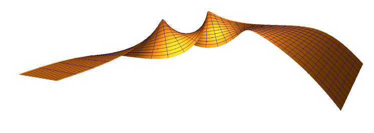
Figure 1: A simultaneously bent and twisted strip.

The structure of the paper is as follows. In Section 2 we introduce the Dirichlet Laplacian in strips on ruled surfaces in any space dimension under minimal regularity hypotheses. The essential spectrum of asymptotically flat strips is located in Section 3. The effects of bending and twisting are investigated in Sections 4 and 5, respectively. In Section 6 we show that, in the limit when the width of the strip tends to zero, the Dirichlet Laplacian converges in a norm resolvent sense to a one-dimensional Schrödinger operator whose potential contains information about the deformations of twisting and bending. Appendix A is devoted to the construction of a relatively parallel adapted frame for an arbitrary curve.

2 Definition of quantum strips

2.1 The reference curve

Given any positive integer $n$, let $\Gamma:\mathbb{R}\to\mathbb{R}^{n+1}$ be a curve of class $C^{1,1}$ which is (without loss of generality) parameterised by its arc-length (i.e. $|\Gamma^{\prime}(s)|=1$ for all $s\in\mathbb{R}$). By the regularity hypothesis, the tangent vector field $T\vcentcolon=\Gamma^{\prime}$ is differentiable almost everywhere. Moreover, in Appendix A, we show that there exist $n$ almost-everywhere differentiable normal vector fields $N_{1},\dots,N_{n}$ such that

$$\begin{pmatrix}T\\ N_{1}\\ \vdots\\ N_{n}\end{pmatrix}^{\prime}=\begin{pmatrix}0&k_{1}&\dots&k_{n}\\ -k_{1}&0&\dots&0\\ \vdots&\vdots&\ddots&\vdots\\ -k_{n}&0&\dots&0\end{pmatrix}\begin{pmatrix}T\\ N_{1}\\ \vdots\\ N_{n}\end{pmatrix},$$ (2.1)

where $k_{1},\dots,k_{n}:\mathbb{R}\to\mathbb{R}$ are locally bounded functions. Introducing the $n$-tuple $k\vcentcolon=(k_{1},\dots,k_{n})$ and calling it the curvature vector, we have $k_{1}^{2}+\dots+k_{n}^{2}=\kappa^{2}$ with $\kappa\vcentcolon=|\Gamma^{\prime\prime}|$ being the curvature of $\Gamma$.

Since the derivative $N_{j}^{\prime}$ is tangential for every $j\in\{1,\dots,n\}$, the normal vectors rotate along the curve $\Gamma$ only whatever amount is necessary to remain normal. In fact, each normal vector $N_{j}$ is translated along $\Gamma$ as close to a parallel transport as possible without losing normality. For this reason, and in analogy with the three-dimensional setting [2], each vector field $N_{j}$ is called relatively parallel and the $(n+1)$-tuple $(T,N_{1},\dots,N_{n})$ is called a relatively parallel adapted frame. Notice that contrary to the standard Frenet frame which requires a higher regularity $C^{n+1}$ and the non-degeneracy condition $\kappa>0$, the relatively parallel adapted frame always exists under the minimal hypothesis $C^{1,1}$.

2.2 The strip as a surface in the Euclidean space

Recall the definition $\Omega_{0}\vcentcolon=\mathbb{R}\times(-a,a)$ for a straight strip. Isometrically embedding $\Omega_{0}$ to $\mathbb{R}^{n+1}$, we can think of $\Omega_{0}$ as a surface in $\mathbb{R}^{n+1}$ obtained by parallelly translating the segment $(-a,a)$ along a straight line. We define a general curved strip $\Omega$ in $\mathbb{R}^{n+1}$ as the ruled surface obtained by translating the segment $(-a,a)$ along $\Gamma$ with respect to a generic normal field

$$N_{\Theta}\vcentcolon=\Theta_{1}N_{1}+\dots+\Theta_{n}N_{n}\,,$$ (2.2)

where $\Theta_{j}:\mathbb{R}\to\mathbb{R}$ with $j\in\{1,\dots,n\}$ are such scalar functions that $\Theta_{j}\in C^{0,1}(\mathbb{R})$ and

$$\Theta_{1}^{2}+\dots+\Theta_{n}^{2}=1\,.$$ (2.3)

More specifically, we set

$$\Omega\vcentcolon=\big{\{}\Gamma(s)+N_{\Theta}(s)\,t:\ (s,t)\in\Omega_{0}\big{\}}\,.$$ (2.4)

In this way, $\Omega$ can be clearly understood as a deformation of the straight strip $\Omega_{0}$, see Figure 1.

We construct the $n$-tuple $\Theta\vcentcolon=(\Theta_{1},\dots,\Theta_{n})$ and call it the twisting vector. We naturally write $|\Theta^{\prime}|\vcentcolon=(\Theta_{1}^{\prime 2}+\dots+\Theta_{n}^{\prime 2})^{1/2}$. If the twisting vector $\Theta$ is constant, i.e. $\Theta^{\prime}=0$, so that the vector field $N_{\Theta}$ is relatively parallel, we say that the strip $\Omega$ is untwisted or purely bent (including the trivial situation $\kappa=0$ when $\Omega$ can be identified with the straight strip $\Omega_{0}$). See Figure 2 for a purely bent planar strip and Figure 5 (middle) for a purely bent non-planar strip.

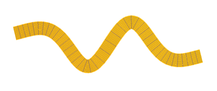
Figure 2: A purely bent (planar) strip.

On the other hand, if the scalar product of the curvature and twisting vectors vanishes, i.e. $k\cdot\Theta\vcentcolon=k_{1}\Theta_{1}+\dots+k_{n}\Theta_{n}=0$, we say that the strip is unbent or purely twisted (including again the trivial situation $\kappa=0$ and $\Theta^{\prime}=0$ when $\Omega$ can be identified with the straight strip $\Omega_{0}$). See Figure 3 for a purely twisted strip along a straight line and Figure 5 (right) for a purely twisted strip along a space curve.

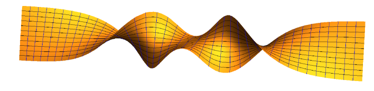
Figure 3: A purely twisted strip.

Notice that unbent and untwisted does not necessarily mean that $\Omega$ and $\Omega_{0}$ are isometric (think of a planar non-straight curve $\Gamma$ in $\mathbb{R}^{3}$ and choose for $N_{\Theta}$ the binormal vector field), see Figure 4.

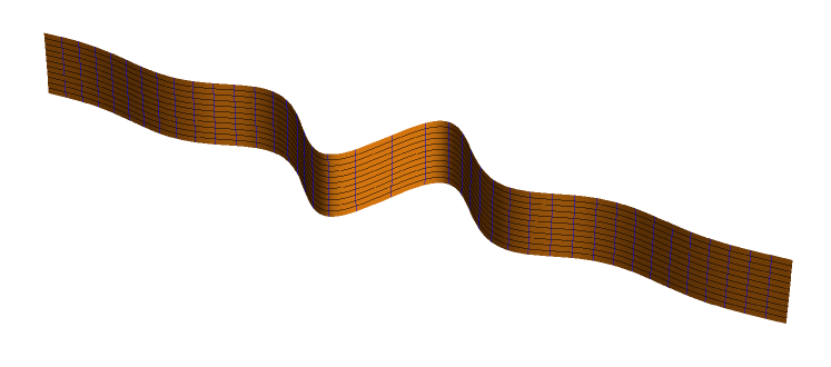
Figure 4: An unbent untwisted strip.

Finally, Figure 5 provides an example of a (non-planar) bent strip, which is twisted or untwisted according to whether $N_{\Theta}$ is relatively parallel or not, respectively.

Remark 2.1.

Let us provide geometrical interpretations to the crucial quantities $k\cdot\Theta$ and $\Theta^{\prime}$ and supporting in this way the terminology introduced above. Interpreting $\Gamma$ as a curve on the surface $\Omega$, it is easily seen that $k\cdot\Theta$ is just the geodesic curvature of $\Gamma$. Hence, the strip is unbent if, and only if, $\Gamma$ is a geodesic on $\Omega$. At the same time, the Gauss curvature of the surface $\Omega$ equals $-|\Theta^{\prime}|^{2}/f^{4}$, where $f$ is given in (2.6) below. In accordance with a general result for ruled surfaces (cf. [18, Prop. 3.7.5]), we observe that this intrinsic curvature of the ambient manifold $\Omega$ is always non-positive. Moreover, the strip is untwisted if, and only if, the surface $\Omega$ is flat in the sense that the Gauss curvature is identically equal to zero.

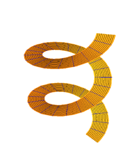
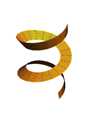
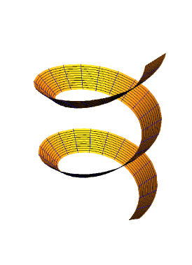
  $k\cdot\Theta\not=0\ \land\ \Theta^{\prime}\not=0$ $k\cdot\Theta\not=0\ \land\ \Theta^{\prime}=0$ $k\cdot\Theta=0\ \land\ \Theta^{\prime}\not=0$

Figure 5: Strips built along a helix. Left: simultaneously bent and twisted version (the principal normal of the Frenet frame is used). Middle: bent and untwisted version (a relatively parallel frame is used). Right: unbent and twisted version (a sum of the principal normal and binormal of the Frenet frame is used).

2.3 The strip as a Riemannian manifold

Further conditions must be imposed on the geometry of $\Omega$ in order to identify the curved strip with a Riemannian manifold. To this aim, let us introduce the mapping $\mathscr{L}:\mathbb{R}^{2}\to\mathbb{R}^{n+1}$ defined by (cf. (2.4))

$$\mathscr{L}(s,t)\vcentcolon=\Gamma(s)+N_{\Theta}(s)\,t\,,$$ (2.5)

so that $\Omega=\mathscr{L}(\Omega_{0})$. The blue segments in the figures represent the geodesics $t\mapsto\mathscr{L}(s,t)$ for various choices of $s$, while the black lines correspond to the curves $s\mapsto\mathscr{L}(s,t)$ parallel to $\Gamma$ at distance $|t|$.

Consider the metric $g\vcentcolon=\nabla\mathscr{L}\cdot(\nabla\mathscr{L})^{T}$, where the dot denotes the scalar product in $\mathbb{R}^{n+1}$. A simple computation using (2.1) yields

$$g=\begin{pmatrix}f^{2}&0\\ 0&1\end{pmatrix}\qquad\mbox{with}\qquad f(s,t)\vcentcolon=\sqrt{\big{[}1-t\,k(s)\cdot\Theta(s)\big{]}^{2}+t^{2}\,|\Theta^{\prime}(s)|^{2}}\,.$$ (2.6)

Let us now strengthen our standing hypotheses.

Assumption 1.

Let $\Gamma\in C^{1,1}(\mathbb{R};\mathbb{R}^{n+1})$ and $\Theta\in C^{0,1}(\mathbb{R};\mathbb{R}^{n})$. Suppose (2.3), $k\cdot\Theta\in L^{\infty}(\mathbb{R})$ and $$a\,\|k\cdot\Theta\|_{L^{\infty}(\mathbb{R})}<1\,.$$

It follows from Assumption 1 that the Jacobian $f$ never vanishes, namely

$$f(s,t)\geq 1-a\,\|k\cdot\Theta\|_{L^{\infty}(\mathbb{R})}>0$$ (2.7)

for almost every $(s,t)\in\Omega_{0}$. If $\Gamma$ and $\Theta$ were smooth functions, the inverse function theorem would immediately imply that $\mathscr{L}:\Omega_{0}\to\Omega$ is a local smooth diffeomorphism, so that $\Omega$ could be identified with the Riemannian manifold $(\Omega_{0},g)$, with $\mathscr{L}$ realising an immersion in $\mathbb{R}^{n+1}$. Under our minimal regularity assumptions, however, we have to be rather careful.

Proposition 2.2.

Suppose Assumption 1. Then $\mathscr{L}:\Omega_{0}\to\Omega$ is a local $C^{0,1}$-diffeomorphism.

Proof.

Given any bounded interval $I\subset\mathbb{R}$, let $s_{1},s_{2}\in I$ and $t_{1},t_{2}\in(-a,a)$. Let us look at the difference

$$\mathscr{L}(s_{2},t_{2})-\mathscr{L}(s_{1},t_{1}) =\Gamma(s_{2})-\Gamma(s_{1})+N_{\Theta}(s_{2})\,t_{2}-N_{\Theta}(s_{1})\,t_{1}$$

$$=\int_{s_{1}}^{s_{2}}T(\xi)\,\mathrm{d}\xi+(t_{2}-t_{1})\,N_{\Theta}(s_{1})+t_{2}\int_{s_{1}}^{s_{2}}N_{\Theta}^{\prime}(\xi)\,\mathrm{d}\xi$$

$$=\int_{s_{1}}^{s_{2}}\Big{(}\big{[}1-t_{2}\,(k\cdot\Theta)(\xi)\big{]}\,T(\xi)+\big{[}t_{2}\,(\Theta^{\prime}\cdot N)(\xi)\big{]}\Big{)}\,\mathrm{d}\xi+(t_{2}-t_{1})\,N_{\Theta}(s_{1})\,,$$

where we have used (2.2) and (2.1) and abbreviated $\Theta^{\prime}\cdot N\vcentcolon=\Theta_{1}^{\prime}N_{1}+\dots+\Theta_{n}^{\prime}N_{n}$. From the identity on the last line, we immediately conclude that

$$|\mathscr{L}(s_{2},t_{2})-\mathscr{L}(s_{1},t_{1})|\leq\big{[}(1+a\,\|k\cdot\Theta\|_{\infty})+a\,\|\Theta^{\prime}\|_{\infty}\big{]}\,|s_{2}-s_{1}|+|t_{1}-t_{1}|\,,$$

where $\|\cdot\|_{\infty}$ denotes the supremum norm of $L^{\infty}(I)$ and $\|\Theta^{\prime}\|_{\infty}\vcentcolon=\||\Theta^{\prime}|\|_{\infty}$. Since the choice of the interval $I$ has been arbitrary, we conclude that $\mathscr{L}$ is a locally Lipschitz function.

To show that $\mathscr{L}$ is a locally bi-Lipschitz function, i.e. also the inverse $\mathscr{L}^{-1}$ is a Lipschitz function on $I\times(-a,a)$, we further improve the expansions above to

$$\Gamma(s_{2})-\Gamma(s_{1}) =T(s_{1})\,(s_{2}-s_{1})+\int_{s_{1}}^{s_{2}}\int_{s_{1}}^{\xi}(k\cdot N)(\eta)\,\mathrm{d}\eta\,\mathrm{d}\xi\,,$$

$$\int_{s_{1}}^{s_{2}}N_{\Theta}^{\prime}(\xi)\,\mathrm{d}\xi =N(s_{1})\cdot\int_{s_{1}}^{s_{2}}\Theta^{\prime}(\xi)\,\mathrm{d}\xi-T(s_{1})\int_{s_{1}}^{s_{2}}(k\cdot\Theta)(\xi)\,\mathrm{d}\xi$$

$$\quad+\int_{s_{1}}^{s_{2}}\int_{s_{1}}^{\xi}\Theta^{\prime}(\xi)\cdot N^{\prime}(\eta)\,\mathrm{d}\eta\,\mathrm{d}\xi-\int_{s_{1}}^{s_{2}}\int_{s_{1}}^{\xi}(k\cdot\Theta)(\xi)\,T^{\prime}(\eta)\,\mathrm{d}\eta\,\mathrm{d}\xi\,.$$

That is, we can write $\mathscr{L}(s_{2},t_{2})-\mathscr{L}(s_{1},t_{1})=A+B$ with

$$A \vcentcolon=T(s_{1})\left[(s_{2}-s_{1})-t_{2}\int_{s_{1}}^{s_{2}}(k\cdot\Theta)(\xi)\,\mathrm{d}\xi\right]+N(s_{1})\cdot\left[(t_{2}-t_{1})\,\Theta(s_{1})+t_{2}\int_{s_{1}}^{s_{2}}\Theta^{\prime}(\xi)\,\mathrm{d}\xi\right],$$

$$B \vcentcolon=\int_{s_{1}}^{s_{2}}\int_{s_{1}}^{\xi}(k\cdot N)(\eta)\,\mathrm{d}\eta\,\mathrm{d}\xi+t_{2}\int_{s_{1}}^{s_{2}}\int_{s_{1}}^{\xi}\Theta^{\prime}(\xi)\cdot N^{\prime}(\eta)\,\mathrm{d}\eta\,\mathrm{d}\xi-t_{2}\int_{s_{1}}^{s_{2}}\int_{s_{1}}^{\xi}(k\cdot\Theta)(\xi)\,T^{\prime}(\eta)\,\mathrm{d}\eta\,\mathrm{d}\xi\,.$$

For every $\delta_{1},\delta_{2}\in(0,1)$, we have

$$|A|^{2} =\left[(s_{2}-s_{1})-t_{2}\int_{s_{1}}^{s_{2}}(k\cdot\Theta)(\xi)\,\mathrm{d}\xi\right]^{2}+\left[(t_{2}-t_{1})\,\Theta(s_{1})+t_{2}\int_{s_{1}}^{s_{2}}\Theta^{\prime}(\xi)\,\mathrm{d}\xi\right]^{2}$$

$$\geq\delta_{1}\,(s_{2}-s_{1})^{2}-\frac{\delta_{1}}{1-\delta_{1}}\,a^{2}\,\|k\cdot\Theta\|_{\infty}^{2}\,(s_{2}-s_{1})^{2}+\delta_{2}\,(t_{2}-t_{1})^{2}-\frac{\delta_{2}}{1-\delta_{2}}\,a^{2}\,\|\Theta^{\prime}\|_{\infty}^{2}\,(s_{2}-s_{1})^{2}$$

$$=\delta_{1}\,(s_{2}-s_{1})^{2}\,\left[1-\frac{1}{1-\delta_{1}}\,a^{2}\,\|k\cdot\Theta\|_{\infty}^{2}-\frac{\delta_{2}/\delta_{1}}{1-\delta_{2}}\,a^{2}\,\|\Theta^{\prime}\|_{\infty}^{2}\right]+\delta_{2}\,(t_{2}-t_{1})^{2}\,.$$

By Assumption 1, we can choose $\delta_{1}$ so small that $1-\frac{1}{1-\delta_{1}}\,a^{2}\,\|k\cdot\Theta\|_{\infty}^{2}$ is positive. Then we choose $\delta_{2}$ so small that the square bracket in the last line above is positive. Altogether we can assure that there is a positive constant $c$, depending exclusively on the choice of the interval $I$, such that

$$|A|\geq c\sqrt{(s_{2}-s_{1})^{2}+(t_{2}-t_{1})^{2}}\,.$$

At the same time, using (2.1), we have

$$|B|\leq(s_{2}-s_{1})^{2}\left(\|\kappa\|_{\infty}+a\,\|\Theta^{\prime}\|_{\infty}\|\kappa\|_{\infty}+a\,\|\kappa\|_{\infty}^{2}\right).$$

Notice that $\|\kappa\|_{\infty}$ is finite by Assumption 1, although $\kappa$ is not supposed to be necessarily bounded on $\mathbb{R}$. That is, there exists a positive constant $C$, depending exclusively on the choice of the interval $I$, such that $|B|\leq C|I||s_{2}-s_{1}|$, where $|I|$ denotes the length of the interval $I$. Consequently,

$$|\mathscr{L}(s_{2},t_{2})-\mathscr{L}(s_{1},t_{1})|\geq(c-C|I|)\sqrt{(s_{2}-s_{1})^{2}+(t_{2}-t_{1})^{2}}$$

for all $s_{1},s_{2}\in I$ and $t_{1},t_{2}\in(-a,a)$. Choosing $|I|$ sufficiently small, we see that $\mathscr{L}$ is invertible on $I\times(-a,a)$ and that the inverse $\mathscr{L}^{-1}$ is a locally Lipschitz function. ∎

As a consequence of this proposition, the restriction $\mathscr{L}\upharpoonright\Omega_{0}$ is a $C^{0,1}$-immersion. Assuming additionally that $\mathscr{L}\upharpoonright\Omega_{0}$ is injective, then it is actually an embedding and $\Omega$ has a geometrical meaning of a non-self-intersecting strip. For our purposes, however, it is enough to assume that $\Omega$ is an immersed submanifold. Even less, disregarding the ambient space $\mathbb{R}^{n+1}$ completely, instead of $\Omega$ we shall consider $(\Omega_{0},g)$ as an abstract Riemannian manifold. From now on, we thus assume the minimal hypotheses of Assumption 1 and nothing more.

Remark 2.3.

It is worth noticing that, contrary to the geodesic curvature $k\cdot\Theta$, the curvature $\kappa$ is not assumed to be (globally) bounded by Assumption 1. In particular, $\Gamma$ is allowed to be a spiral with $\kappa(s)\to\infty$ as $s\to\pm\infty$.

2.4 The strip as a quantum Hamiltonian

The word “quantum” refers to that we consider the Hamiltonian of a free quantum particle constrained to $\Omega$. As usual, we model the Hamiltonian by the Laplace-Beltrami operator in $L^{2}(\Omega)$, subject to Dirichlet boundary condition. Since we think of $\Omega$ as part of an abstract manifold (not necessarily embedded in $\mathbb{R}^{n+1}$), we disregard the presence of extrinsic potentials occasionally added to the Laplace-Beltrami operator in order to justify quantisation on submanifolds (cf. [13]).

Using the identification $\Omega\cong(\Omega_{0},g)$ with the metric $g$ given by (2.6), the operator of our interest is thus the self-adjoint operator $H$ in the Hilbert space

$$\mathcal{H}\vcentcolon=L^{2}(\Omega_{0},|g(s,t)|^{1/2}\,\mathrm{d}s\,\mathrm{d}t)=L^{2}(\Omega_{0},f(s,t)\,\mathrm{d}s\,\mathrm{d}t)$$ (2.8)

that acts as

$$-\Delta_{g}\vcentcolon=-|g|^{1/2}\partial_{\mu}|g|^{1/2}g^{\mu\nu}\partial_{\nu}=-f^{-1}\,\partial_{1}\,f^{-1}\,\partial_{1}-f^{-1}\,\partial_{2}\,f\,\partial_{2}$$ (2.9)

in $\Omega_{0}$ and the functions in the operator domain vanish on $\partial\Omega_{0}$. Here we employ the standard notations $|g|\vcentcolon=\det(g)$ and $(g^{\mu\nu})=g^{-1}$ together with the Einstein summation convention with the range of indices being $\mu,\nu\in\{1,2\}$. As usual we introduce $H$ as the Friedrichs extension of the operator $-\Delta_{g}$ initially defined on $C_{0}^{\infty}(\Omega_{0})$. More specifically, $H$ is defined as the self-adjoint operator associated in $\mathcal{H}$ (in the sense of the representation theorem [16, Thm. VI.2.1]) with the quadratic form

$$h[\psi] \vcentcolon=\|f^{-1/2}\partial_{1}\psi\|_{\mathcal{H}}^{2}+\|f^{1/2}\partial_{2}\psi\|_{\mathcal{H}}^{2}=\int_{\Omega_{0}}\frac{|\partial_{1}\psi(s,t)|^{2}}{f(s,t)}\,\mathrm{d}s\,\mathrm{d}t+\int_{\Omega_{0}}|\partial_{2}\psi(s,t)|^{2}\,f(s,t)\,\mathrm{d}s\,\mathrm{d}t\,,$$ (2.10)

$$\mathrm{Dom}(h) \vcentcolon=\overline{C_{0}^{\infty}(\Omega_{0})}^{\|\cdot\|_{\mathcal{H}_{1}}}\,,\qquad\mbox{where}\qquad\|\psi\|_{\mathcal{H}_{1}}\vcentcolon=\sqrt{h[\psi]+\|\psi\|_{\mathcal{H}}^{2}}\,.$$

By $\mathcal{H}_{1}$ we shall understand the Hilbert space $\mathrm{Dom}(h)$ equipped with the norm $\|\cdot\|_{\mathcal{H}_{1}}$.

Under our standing hypotheses of Assumption 1, the crucial bound (2.7) holds and, moreover, the function $f$ is locally bounded. Consequently, one has

$$\{\psi\in W_{0}^{1,2}(\Omega_{0}):\ \mathop{\mathrm{supp}}\nolimits\psi\subset[-R,R]\times[-a,a]\mbox{ for some }R>0\}\subset\mathrm{Dom}(h)\,.$$ (2.11)

Assuming in addition that

$$|\Theta^{\prime}|\in L^{\infty}(\mathbb{R})\,,$$ (2.12)

then there exists a positive constant $C$ such that even the global bounds

$$C^{-1}\leq f(s,t)\leq C$$ (2.13)

hold for almost every $(s,t)\in\Omega_{0}$. Consequently, $\|\cdot\|_{\mathcal{H}_{1}}$ is equivalent to the usual norm of the Sobolev space $W^{1,2}(\Omega_{0})$ and one has $\mathrm{Dom}(h)=W_{0}^{1,2}(\Omega_{0})$. In this paper, however, we proceed in a greater generality without assuming the extra hypothesis (2.12).

3 Asymptotically flat strips

If the strip $\Omega$ is flat in the sense that its metric (2.6) is Euclidean, i.e. $f=1$ (identically), then $H$ coincides with the Dirichlet Laplacian in $\Omega_{0}$, which we denote here by $H_{0}$. More specifically, $H_{0}$ is the operator in $\mathcal{H}_{0}\vcentcolon=L^{2}(\Omega_{0})$ associated with the quadratic form $h_{0}[\psi]\vcentcolon=\int_{\Omega_{0}}|\nabla\psi(x)|^{2}\,\mathrm{d}x$, $\mathrm{Dom}(h_{0})\vcentcolon=W_{0}^{1,2}(\Omega_{0})$. It is well known that

$$\sigma(H_{0})=[E_{1},\infty)\qquad\mbox{with}\qquad E_{1}\vcentcolon=\left(\frac{\pi}{2a}\right)^{2}$$

and that the (purely essential) spectrum is in fact purely absolutely continuous.

In this section, we consider quantum strips which are asymptotically flat in the sense that their metric (2.6) converges to the flat metric at the infinity of $\Omega_{0}$. More specifically, we impose the conditions

$$\lim_{|s|\to\infty}(k\cdot\Theta)(s)=0\qquad\mbox{and}\qquad\lim_{|s|\to\infty}|\Theta^{\prime}(s)|=0\,.$$ (3.1)

Since quantum propagating states are expected to be determined by the behaviour of the metric at infinity, the following result is very intuitive.

Theorem 3.1.

Suppose Assumption 1. If (3.1) holds, then

$$\sigma_{\mathrm{ess}}(H)=[E_{1},\infty)\,.$$

We establish the theorem as a consequence of two lemmata. First we show that the energy of the propagating states cannot descend below $E_{1}$.

Lemma 3.2.

Suppose Assumption 1. If (3.1) holds, then

$$\inf\sigma_{\mathrm{ess}}(H)\geq E_{1}\,.$$

Proof.

Given any arbitrary positive number $s_{0}$, we divide $\Omega_{0}$ into an interior and an exterior part with respect to $s_{0}$ as follows:

$$\Omega_{0,\mathrm{int}}\vcentcolon=(-s_{0},s_{0})\times(-a,a)\,,\qquad\Omega_{0,\mathrm{ext}}\vcentcolon=\Omega_{0}\setminus\overline{\Omega_{0,\mathrm{int}}}\,.$$

Imposing Neumann boundary conditions on the segments $\{\pm s_{0}\}\times(-a,a)$, one gets the lower bound

$$H\geq H^{N}\vcentcolon=H^{N}_{\mathrm{int}}\oplus H^{N}_{\mathrm{ext}}$$ (3.2)

in the sense of forms in $\mathcal{H}$. Here $H^{N}_{\mathrm{int}}$ is the operator in $\mathcal{H}_{\mathrm{int}}\vcentcolon=L^{2}(\Omega_{0,\mathrm{int}},f(s,t)\,\mathrm{d}s\,\mathrm{d}t)$ associated with the quadratic form $h_{\mathrm{int}}^{N}$ that acts as $h$ but whose domain is restricted to $\Omega_{0,\mathrm{int}}$. More specifically,

$$h_{\mathrm{int}}^{N}[\psi] \vcentcolon=\int_{\Omega_{0,\mathrm{int}}}\frac{|\partial_{1}\psi(s,t)|^{2}}{f(s,t)}\,\mathrm{d}s\,\mathrm{d}t+\int_{\Omega_{0,\mathrm{int}}}|\partial_{2}\psi(s,t)|^{2}\,f(s,t)\,\mathrm{d}s\,\mathrm{d}t\,,$$

$$\mathrm{Dom}(h_{\mathrm{int}}^{N}) \vcentcolon=\left\{\psi\vcentcolon=\tilde{\psi}\upharpoonright\Omega_{0,\mathrm{int}}:\ \tilde{\psi}\in\mathrm{Dom}(h)\right\}\,.$$

Note that no boundary conditions are imposed on the parts $\{\pm s_{0}\}\times(-a,a)$ of the boundary $\partial\Omega_{0,\mathrm{int}}$ in the form domain, while Dirichle boundary conditions are considered on the remaining parts of the boundary. The operator $H^{N}_{\mathrm{ext}}$, the form $h^{N}_{\mathrm{ext}}$ and the Hilbert space $\mathcal{H}_{\mathrm{ext}}$ are defined analogously.

Employing the Neumann bracketing described above, we have

$$\inf\sigma_{\mathrm{ess}}(H)\geq\inf\sigma_{\mathrm{ess}}(H^{N})=\inf\sigma_{\mathrm{ess}}(H^{N}_{\mathrm{ext}})\geq\inf\sigma(H^{N}_{\mathrm{ext}})\,.$$

Here the first inequality follows from (3.2) via the minimax principle, the equality is due to the fact that the spectrum of $H^{N}_{\mathrm{int}}$ is purely discrete and the last inequality is trivial. Hence, it is sufficient to find a suitable lower bound to the spectrum of $H^{N}_{\mathrm{ext}}$. To this aim, for every $\psi\in\mathrm{Dom}(h_{\mathrm{ext}}^{N})$, we estimate the quadratic form as follows:

$$h^{N}_{\mathrm{ext}}[\psi] \geq\int_{\Omega_{0,\mathrm{ext}}}|\partial_{2}\psi(s,t)|^{2}\,f(s,t)\,\mathrm{d}s\,\mathrm{d}t$$

$$\geq\big{(}\mathop{\mathrm{ess\;\!inf}}_{\Omega_{0,\mathrm{ext}}}f\big{)}\int_{\Omega_{0,\mathrm{ext}}}|\partial_{2}\psi(s,t)|^{2}\,\mathrm{d}s\,\mathrm{d}t$$

$$\geq E_{1}\,\big{(}\mathop{\mathrm{ess\;\!inf}}_{\Omega_{0,\mathrm{ext}}}f\big{)}\int_{\Omega_{0,\mathrm{ext}}}|\psi(s,t)|^{2}\,\mathrm{d}s\,\mathrm{d}t$$

$$\geq E_{1}\,\big{(}\mathop{\mathrm{ess\;\!inf}}_{\Omega_{0,\mathrm{ext}}}f\big{)}\,\big{(}\mathop{\mathrm{ess\;\!sup}}_{\Omega_{0,\mathrm{ext}}}f\big{)}^{-1}\int_{\Omega_{0,\mathrm{ext}}}|\psi(s,t)|^{2}\,f(s,t)\,\mathrm{d}s\,\mathrm{d}t$$

$$=E_{1}\,\big{(}\mathop{\mathrm{ess\;\!inf}}_{\Omega_{0,\mathrm{ext}}}f\big{)}\,\big{(}\mathop{\mathrm{ess\;\!sup}}_{\Omega_{0,\mathrm{ext}}}f\big{)}^{-1}\|\psi\|^{2}_{\mathcal{H}_{\mathrm{ext}}}\,.$$

Consequently,

$$\inf\sigma_{\mathrm{ess}}(H)\geq E_{1}\,\big{(}\mathop{\mathrm{ess\;\!inf}}_{\Omega_{0,\mathrm{ext}}}f\big{)}\,\big{(}\mathop{\mathrm{ess\;\!sup}}_{\Omega_{0,\mathrm{ext}}}f\big{)}^{-1}\,.$$

Taking the limit $s_{0}\to\infty$, the asymptotic hypothesis (3.1) ensures that the right-hand side tends to $E_{1}$, while the left-hand side is independent of $s_{0}$. This concludes the proof of the lemma. ∎

It remains to show that all energies above $E_{1}$ belong to the essential spectrum.

Lemma 3.3.

Suppose Assumption 1. If (3.1) holds, then

$$\sigma_{\mathrm{ess}}(H)\supset[E_{1},\infty)\,.$$

Proof.

Our argument is based on the Weyl criterion adapted to quadratic forms (see [26, Thm. 5] for the proof of the criterion and [25, Lem. 5.3] for an original application to quantum waveguides). It states that to prove that $\eta$ is in the spectrum of the operator $H$, it is enough to find a sequence $\{\psi_{n}\}_{n\in\mathbb{N}}\subset\mathrm{Dom}\left(h\right)$ such that

1. $\displaystyle\liminf_{n\to\infty}\|\psi_{n}\|_{\mathcal{H}}>0$,

2. $\displaystyle\lim_{n\to\infty}\|\left(H-\eta\right)\psi_{n}\|_{\mathcal{H}_{-1}}=0$,

where $\mathcal{H}_{-1}$ denotes the dual space of $\mathcal{H}_{1}$. Notice that the mapping $H+1:\mathcal{H}_{1}\to\mathcal{H}_{-1}$ is an isomorphism and that the dual norm is given by

$$\|\psi\|_{\mathcal{H}_{-1}}=\sup_{\stackrel{{\scriptstyle[}}{{\phi}}\not=0]{}{\phi\in\mathrm{Dom}\left(h\right)}}\frac{|\tensor[_{\mathcal{H}_{1}}]{(\phi,\psi)}{{}_{\mathcal{H}_{-1}}}|}{\|\phi\|_{\mathcal{H}_{1}}}\,,$$

where $\tensor[_{\mathcal{H}_{1}}]{(\cdot,\cdot)}{{}_{\mathcal{H}_{-1}}}$ denotes the duality pairing between $\mathcal{H}_{1}$ and $\mathcal{H}_{-1}$. In contrast to the conventional Weyl criterion, the advantage of this characterisation is that the sequence is required to lie in the form domain only and the limit in (ii) is taken in the weaker topology of $\mathcal{H}_{-1}$.

We parameterise $\eta$ by setting $\eta=\lambda^{2}+E_{1}$ with any $\lambda\in\mathbb{R}$. Note that the differential equations $-\Delta\psi=\eta\psi$ is solved by $(s,t)\mapsto\chi_{1}\left(t\right)\mathrm{e}^{i\lambda s}$, where

$$\chi_{1}(t)\vcentcolon=\sqrt{\frac{1}{a}}\,\cos\big{(}\sqrt{E_{1}}t\big{)}$$ (3.3)

denotes the normalised eigenfunction of the Dirichlet Laplacian in $(-a,a)$ corresponding to the eigenvalue $E_{1}$. However, this solution does not even belong to $\mathcal{H}$. To get an approximate solution which simultaneously belongs to $\mathrm{Dom}(h)$ and is “localised at infinity”, for every $n\in\mathbb{N}\vcentcolon=\{1,2,\dots\}$ we set

$$\varphi_{n}\left(s\right)\vcentcolon=\frac{1}{\sqrt{n}}\,\varphi\left(\frac{s}{n}-n\right),$$

where $\varphi\in C_{0}^{\infty}(\mathbb{R})$ is any function such that $\mathop{\mathrm{supp}}\nolimits\varphi\subset\left(-1,1\right)$ and $\|\varphi\|_{L^{2}(\mathbb{R})}=1$. The normalisation factor is chosen in such a way that

$$\|\varphi_{n}\|_{L^{2}(\mathbb{R})}=\|\varphi\|_{L^{2}(\mathbb{R})}=1\,,\qquad\|\varphi_{n}^{\prime}\|_{L^{2}(\mathbb{R})}=n^{-1}\,\|\varphi^{\prime}\|_{L^{2}(\mathbb{R})}\,,\qquad\|\varphi_{n}^{\prime\prime}\|_{L^{2}(\mathbb{R})}=n^{-2}\,\|\varphi^{\prime\prime}\|_{L^{2}(\mathbb{R})}\,.$$ (3.4)

Notice also that $\mathop{\mathrm{supp}}\nolimits\varphi_{n}\subset\left(n^{2}-n,n^{2}+n\right)$. We then define

$$\psi_{n}\left(s,t\right)\vcentcolon=\varphi_{n}\left(s\right)\chi_{1}\left(t\right)\mathrm{e}^{i\lambda s}\,.$$

Recalling (2.11), we clearly have $\psi_{n}\in\mathrm{Dom}(h)$ for every $n\in\mathbb{N}$. Our aim is to show that $\{\psi_{n}\}_{n\in\mathbb{N}}$ satisfies conditions (i) and (ii) of the modified Weyl criterion.

First of all, notice that, due to (2.7) and the normalisations of $\varphi$ and $\chi_{1}$, we have

$$\|\psi_{n}\|_{\mathcal{H}}^{2}\geq 1-a\,\|k\cdot\Theta\|_{L^{\infty}(\mathbb{R})}>0\,,$$

so the condition (i) clearly holds. Next, for every $\phi\in\mathrm{Dom}(h)$, we have

$$|\tensor[_{\mathcal{H}_{1}}]{(\phi,(H-\eta)\psi_{n})}{{}_{\mathcal{H}_{-1}}}| =|h(\phi,\psi_{n})-\eta(\phi,\psi_{n})_{\mathcal{H}}|$$

$$\leq|h_{1}(\phi,\psi_{n})-\lambda^{2}(\phi,\psi_{n})_{\mathcal{H}}|+|h_{2}(\phi,\psi_{n})-E_{1}(\phi,\psi_{n})_{\mathcal{H}}|\,,$$

where, recalling (2.10), $h_{1}[\psi]\vcentcolon=\|f^{-1/2}\partial_{1}\psi\|_{\mathcal{H}}^{2}$, $h_{2}[\psi]\vcentcolon=\|f^{1/2}\partial_{2}\psi\|_{\mathcal{H}}^{2}$, $\mathrm{Dom}(h_{1})\vcentcolon=\mathrm{Dom}(h)=\vcentcolon\mathrm{Dom}(h_{2})$. Integrating by parts and using that $-\chi_{1}^{\prime\prime}=E_{1}\chi_{1}$ together with the normalisations of $\varphi$ and $\chi_{1}$, we have

$$|h_{2}(\phi,\psi_{n})-E_{1}(\phi,\psi_{n})_{\mathcal{H}}| =\left|\int_{\Omega_{0}}\bar{\phi}(s,t)\,\partial_{2}\psi_{n}(s,t)\,\partial_{2}f(s,t)\,\mathrm{d}s\,\mathrm{d}t\right|$$ (3.5)

$$\leq\|\phi\|_{\mathcal{H}}\,\|\partial_{2}\psi_{n}\|_{\mathcal{H}_{0}}\,\left\|\frac{\partial_{2}f}{\sqrt{f}}\right\|_{\infty,n}$$

$$\leq\|\phi\|_{\mathcal{H}_{1}}\,\sqrt{E_{1}}\,\left\|\frac{\partial_{2}f}{\sqrt{f}}\right\|_{\infty,n}\,,$$

where $\|\cdot\|_{\infty,n}\vcentcolon=\|\cdot\|_{L^{\infty}(\mathop{\mathrm{supp}}\nolimits\varphi_{n}\times(-a,a))}$. At the same time, we have

$$h_{1}(\phi,\psi_{n}) =\int_{\Omega_{0}}\partial_{1}\bar{\phi}(s,t)\,\partial_{1}\psi_{n}(s,t)\left[\frac{1}{f(s,t)}-1\right]\mathrm{d}s\,\mathrm{d}t-\int_{\Omega_{0}}\bar{\phi}(s,t)\,\partial_{1}^{2}\psi_{n}(s,t)\,\mathrm{d}s\,\mathrm{d}t\,,$$

$$(\phi,\psi_{n})_{\mathcal{H}} =\int_{\Omega_{0}}\bar{\phi}(s,t)\,\psi_{n}(s,t)\left[f(s,t)-1\right]\mathrm{d}s\,\mathrm{d}t+\int_{\Omega_{0}}\bar{\phi}(s,t)\,\psi_{n}(s,t)\,\mathrm{d}s\,\mathrm{d}t\,.$$

Consequently, using that $-\partial_{1}^{2}\psi_{n}(s,t)-\lambda^{2}\psi_{n}(s,t)=[-\varphi_{n}^{\prime\prime}(s)-2i\lambda\varphi_{n}^{\prime}(s)]\,\mathrm{e}^{i\lambda s}\,\chi_{1}(t)$ and the normalisations of $\varphi$ and $\chi_{1}$ again, we get

$$|h_{1}(\phi,\psi_{n})-\lambda^{2}(\phi,\psi_{n})_{\mathcal{H}}| \leq\|f^{-1/2}\phi\|_{\mathcal{H}}\,\|\partial_{1}\psi_{n}\|_{\mathcal{H}_{0}}\,\left\|\frac{1}{\sqrt{f}}-\sqrt{f}\right\|_{\infty,n}$$ (3.6)

$$\quad+\lambda^{2}\|\phi\|_{\mathcal{H}}\,\|\psi_{n}\|_{\mathcal{H}_{0}}\,\left\|\sqrt{f}-\frac{1}{\sqrt{f}}\right\|_{\infty,n}$$

$$\quad+\|\phi\|_{\mathcal{H}}\,\|\varphi_{n}^{\prime\prime}+2i\lambda\varphi_{n}^{\prime}\|_{L^{2}(\mathbb{R})}\,\left\|\frac{1}{\sqrt{f}}\right\|_{\infty,n}$$

$$\leq\|\phi\|_{\mathcal{H}_{1}}\,\|\varphi_{n}^{\prime}+i\lambda\varphi_{n}\|_{L^{2}(\mathbb{R})}\,\left\|\frac{1}{\sqrt{f}}-\sqrt{f}\right\|_{\infty,n}$$

$$\quad+\lambda^{2}\|\phi\|_{\mathcal{H}_{1}}\,\left\|\sqrt{f}-\frac{1}{\sqrt{f}}\right\|_{\infty,n}$$

$$\quad+\|\phi\|_{\mathcal{H}_{1}}\,\|\varphi_{n}^{\prime\prime}+2i\lambda\varphi_{n}^{\prime}\|_{L^{2}(\mathbb{R})}\,\left\|\frac{1}{\sqrt{f}}\right\|_{\infty,n}\,.$$

Putting (3.5) and (3.6) together, we finally arrive at

$$\|(H-\eta)\psi_{n}\|_{\mathcal{H}_{-1}} \leq\sqrt{E_{1}}\,\left\|\frac{\partial_{2}f}{\sqrt{f}}\right\|_{\infty,n}+\big{(}\|\varphi_{n}^{\prime}+i\lambda\varphi_{n}\|_{L^{2}(\mathbb{R})}+\lambda^{2}\big{)}\left\|\frac{1}{\sqrt{f}}-\sqrt{f}\right\|_{\infty,n}$$

$$\quad+\|\varphi_{n}^{\prime\prime}+2i\lambda\varphi_{n}^{\prime}\|_{L^{2}(\mathbb{R})}\,\left\|\frac{1}{\sqrt{f}}\right\|_{\infty,n}\,.$$

Here the first line on the right-hand side tends to zero as $n\to\infty$ due to (3.1), while the second line vanishes as $n\to\infty$ due to (3.4). This establishes (ii) and the lemma is proved. ∎

Theorem 3.1 follows as a direct consequence of Lemmata 3.2 and 3.3.

4 Purely bent strips

In this section, we consider strips constructed in such a way that the twisting vector $\Theta$ is constant, so that $N_{\Theta}$ is relatively parallel and $\Omega$ is untwisted. We show that the geodesic curvature $k\cdot\Theta$ acts as an attractive interaction in the sense that it diminishes the spectrum. Recall that $k\cdot\Theta$ can be equal to zero even if $\kappa\not=0$ (like, for instance, in Figure 5, right).

Theorem 4.1.

Suppose Assumption 1. If $\Theta^{\prime}=0$ and $k\cdot\Theta\not=0$, then

$$\inf\sigma(H)<E_{1}\,.$$

Proof.

The proof is based on the variational strategy of finding a trial function $\psi\in\mathrm{Dom}(h)$ such that

$$h_{1}[\psi]\vcentcolon=h[\psi]-E_{1}\|\psi\|_{\mathcal{H}}^{2}<0\,.$$ (4.1)

Following [20], we shall achieve the strict inequality by mollifying the first transverse eigenfunction $\chi_{1}$ introduced in (3.3).

Let $\varphi_{1}\in C_{0}^{\infty}(\mathbb{R})$ be a real-valued function such that $0\leq\varphi_{1}\leq 1$, $\varphi_{1}=1$ on $[-1,1]$ and $\varphi_{1}=0$ on $\mathbb{R}\setminus[-2,2]$. Setting $\varphi_{n}(s)\vcentcolon=\varphi_{1}(s/n)$ for every $n\in\mathbb{N}$, we get a family of functions from $W^{1,2}(\mathbb{R})$ such that $\varphi_{n}\to 1$ pointwise as $n\to\infty$ and

$$\|\varphi_{n}^{\prime}\|_{L^{2}(\mathbb{R})}^{2}=n^{-1}\,\|\varphi_{1}^{\prime}\|_{L^{2}(\mathbb{R})}^{2}\xrightarrow[n\to\infty]{}0\,.$$ (4.2)

Defining

$$\psi_{n}(s,t)\vcentcolon=\varphi_{n}(s)\,\chi_{1}(t)$$

and integrating by parts with help of $-\chi_{1}^{\prime\prime}=E_{1}\chi_{1}$, we have

$$h_{1}[\psi_{n}]=\int_{\Omega_{0}}\frac{|\partial_{1}\psi_{n}(s,t)|^{2}}{f(s,t)}\,\mathrm{d}s\,\mathrm{d}t+\frac{1}{2}\int_{\Omega_{0}}|\psi_{n}(s,t)|^{2}\,\partial_{2}^{2}f(s,t)\,\mathrm{d}s\,\mathrm{d}t=\int_{\Omega_{0}}\frac{|\varphi_{n}^{\prime}(s)|^{2}|\chi_{1}(t)|^{2}}{f(s,t)}\,\mathrm{d}s\,\mathrm{d}t\,.$$

Here the second equality follows from the fact that the Jacobian $f$ of the metric (2.6) reduces to

$$f(s,t)=1-t\,k(s)\cdot\Theta(s)$$

provided that $\Theta$ is constant, so it is linear in the second variable and $\partial_{2}^{2}f=0$. Using (2.7) and (4.2), we therefore conclude that

$$\lim_{n\to\infty}h_{1}[\psi_{n}]=0\,.$$ (4.3)

It follows that the functional $h_{1}$ vanishes at $\chi_{1}$ in a generalised sense. The next (and last) step in our strategy is to show that $\chi_{1}$ does not correspond to the minimum of the functional. To this purpose, we add the following asymmetric perturbation

$$\psi_{n,\varepsilon}(s,t)\vcentcolon=\psi_{n}(s,t)+\varepsilon\,\phi(s,t)\,,\qquad\mbox{where}\qquad\phi(s,t)\vcentcolon=\eta(s)\,t\,\chi_{1}(t)\,,$$

with $\varepsilon\in\mathbb{R}$ and $\eta\in C_{0}^{\infty}(\mathbb{R})$ being a non-zero real-valued function to be specified later. Plugging it into the functional, we obviously have

$$h_{1}[\psi_{n,\varepsilon}]=h_{1}[\psi_{n}]+2\,\varepsilon\,h_{1}(\psi_{n},\phi)+\varepsilon^{2}\,h_{1}[\phi]\,.$$ (4.4)

Since $\varphi_{n}=1$ on $\mathop{\mathrm{supp}}\nolimits\eta$ for all sufficiently large $n$, the central term is in fact independent of $n$ and equals

$$h_{1}(\psi_{n},\phi) =\int_{\Omega_{0}}\eta(s)\,\chi_{1}^{\prime}(t)\,[t\,\chi_{1}(t)]^{\prime}\,f(s,t)\,\mathrm{d}s\,\mathrm{d}t-E_{1}\int_{\Omega_{0}}\eta(s)\,t\,|\chi_{1}(t)|^{2}\,f(s,t)\,\mathrm{d}s\,\mathrm{d}t$$

$$=-\int_{\Omega_{0}}\eta(s)\,\chi_{1}^{\prime}(t)\,t\chi_{1}(t)\,\partial_{2}f(s,t)\,\mathrm{d}s\,\mathrm{d}t$$

$$=\frac{1}{2}\int_{\Omega_{0}}\eta(s)\,|\chi_{1}(t)|^{2}\,\partial_{2}f(s,t)\,\mathrm{d}s\,\mathrm{d}t=-\frac{1}{2}\int_{\mathbb{R}}\eta(s)\,(k\cdot\Theta)(s)\,\mathrm{d}s\,.$$

Here the second and third equalities follow by integrations by parts using that $-\chi_{1}^{\prime\prime}=E_{1}\chi_{1}$ and $\partial_{2}^{2}f=0$. Since $k\cdot\Theta$ is not identically equal to zero by the hypothesis of the theorem, it is possible to choose $\eta$ in such a way that the last integral is positive. Summing up, $h_{1}(\psi_{n},\phi)$ equals a negative number for all sufficiently large $n$. Coming back to (4.4), it is thus possible to choose a positive $\varepsilon$ so small that sum of the last two terms on the right-hand side of (4.4) is negative. Then, recalling (4.3), we can choose $n$ so large that $h_{1}[\psi_{n,\varepsilon}]<0$. Hence, $\inf\sigma(H)<0$ by the Rayleigh-Ritz variational characterisation of the lowest point in the spectrum of $H$. ∎

As a consequence of Theorem 4.1, if the strip is in addition asymptotically flat in the sense of (3.1) (of course, just the first limit is relevant under the hypotheses of Theorem 4.1), then the essential spectrum starts by $E_{1}$ (cf. Theorem 3.1) and the spectral threshold $\inf\sigma(H)$ necessarily corresponds to a discrete eigenvalue.

Corollary 4.2.

In addition to the hypotheses of Theorem 4.1, let us assume (3.1). Then

$$\sigma_{\mathrm{disc}}(H)\cap(0,E_{1})\not=\varnothing\,.$$

This is a generalisation of the celebrate result [11] about the existence of quantum bound states in curved planar quantum waveguides.

5 Purely twisted strips

In this section, we consider strips constructed in such a way that $k\cdot\Theta=0$, so that $\Omega$ is unbent. Recall that this hypothesis does not necessarily mean that $\Gamma$ is a straight line (for instance, the setting in Figure 5, right, is admissible). We show that the twisting vector $\Theta$ acts as a repulsive interaction in the sense that it induces Hardy-type inequalities whenever $\Theta^{\prime}$ is not identically equal to zero (but it is not too large).

Theorem 5.1.

Suppose Assumption 1. If $k\cdot\Theta=0$ and $\Theta^{\prime}\not=0$ satisfies

$$a\,\|\Theta^{\prime}\|_{L^{\infty}(\mathbb{R})}\leq\sqrt{2}\,,$$ (5.1)

then there exists a positive constant $c$ such that the inequality

$$H-E_{1}\geq c\,\rho$$ (5.2)

holds in the sense of quadratic forms in $\mathcal{H}$, where $\rho(s,t)\vcentcolon=1/(1+s^{2})$.

To prove the theorem, we follow the strategy of [21]. The main idea is to introduce a function $\lambda:\mathbb{R}\to\mathbb{R}$ by setting

$$\lambda(s)\vcentcolon=\inf_{\stackrel{{\scriptstyle[}}{{\psi}}\not=0]{}{\psi\in W_{0}^{1,2}((-a,a))}}\frac{\displaystyle\int_{-a}^{a}|\psi^{\prime}(t)|^{2}\,f(s,t)\,\,\mathrm{d}t}{\displaystyle\int_{-a}^{a}|\psi(t)|^{2}\,f(s,t)\,\,\mathrm{d}t}-E_{1}\,.$$ (5.3)

We keep the same notation for the function $\lambda\otimes 1$ on $\mathbb{R}\times(-a,a)$. Note that under the assumption $k\cdot\Theta=0$ of this section, the Jacobian $f$ of the metric (2.6) reduces to

$$f(s,t)=\sqrt{1+t^{2}\,\Theta^{\prime}(s)^{2}}\,.$$ (5.4)

The following lemma is the crucial ingredient in the proof of Theorem 5.1.

Lemma 5.2.

Under the assumptions of Theorem 5.1, $\lambda$ is a non-negative non-trivial function.

Proof.

Fix any $s\in\mathbb{R}$. Employing the change of the test function $\phi\vcentcolon=\sqrt{f}\,\psi$ and by integrating by parts, we obtain

$$\lambda(s)=\inf_{\stackrel{{\scriptstyle[}}{{\phi}}\not=0]{}{\phi\in W_{0}^{1,2}((-a,a))}}\frac{\displaystyle\int_{-a}^{a}\left(|\phi^{\prime}(t)|^{2}-E_{1}\,|\phi(t)|^{2}+V(s,t)\,|\phi(t)|^{2}\right)\,\mathrm{d}t}{\displaystyle\int_{-a}^{a}|\phi(t)|^{2}\,\,\mathrm{d}t}$$ (5.5)

with

$$V(s,t)\vcentcolon=\frac{\Theta^{\prime}(s)^{2}\left(2-t^{2}\,\Theta^{\prime}(s)^{2}\right)}{4\,f(s,t)^{4}}\,.$$

We note that $\lambda(s)$ is the spectral threshold of the self-adjoint operator $L$ in $L^{2}((-a,a))$ associated with the closed form

$$l[\phi]\vcentcolon=\int_{-a}^{a}\left(|\phi^{\prime}(t)|^{2}-E_{1}\,|\phi(t)|^{2}+V(s,t)\,|\phi(t)|^{2}\right)\,\mathrm{d}t\,,\qquad\mathrm{Dom}(l)\vcentcolon=W_{0}^{1,2}((-a,a))\,.$$

Since the resolvent of $L$ is compact, $\lambda(s)$ is the lowest eigenvalue of $L$. Let us denote by $\phi_{1}$ a corresponding eigenfunction. By standard arguments (cf. [14, Thm. 8.38]), the eigenvalue is simple and $\phi_{1}$ can be chosen to be positive. The infimum in (5.5) is clearly achieved by $\phi_{1}$. Due to the hypothesis (5.1), the function $V$ is non-negative. At the same time, one has the Poincaré inequality

$$\forall\phi\in W_{0}^{1,2}((-a,a))\,,\qquad\int_{-a}^{a}|\phi^{\prime}(t)|^{2}\,\mathrm{d}t\geq E_{1}\int_{-a}^{a}|\phi(t)|^{2}\,\mathrm{d}t\,.$$ (5.6)

Consequently, $\lambda(s)$ is clearly non-negative. Now, assume that $\lambda(s)=0$. Then necessarily $V(s,t)=0$ for every $t\in(-a,a)$, which implies $\Theta^{\prime}(s)=0$. Since $\Theta^{\prime}$ is supposed not to be identically equal to zero, we necessarily have $\lambda\not=0$ as well. ∎

Using just the definition (5.3) in (2.10), we immediately get the inequality

$$H-E_{1}\geq\lambda\,.$$ (5.7)

By Lemma 5.2, it is a Hardy-type inequality whenever the assumptions of Theorem 5.1 hold true. We call it a local Hardy inequality because the defect of (5.7) is that the right-hand side might not be positive everywhere in $\Omega_{0}$ (like, for instance, if $\Theta^{\prime}$ is compactly supported). To transfer it into the global Hardy inequality (5.2) of Theorem 5.1, we use the longitudinal kinetic energy that we have neglected when deriving (5.7).

Proof of Theorem 5.1.

Let $\psi\in C_{0}^{\infty}(\Omega_{0})$. Under the hypotheses of the theorem, it follows from Lemma 5.2 that $\lambda$ is non-negative and non-trivial. Let us fix any bounded open interval $I\subset\mathbb{R}$ on which $\lambda$ is non-trivial. Let us abbreviate $\Omega_{0}^{I}\vcentcolon=I\times(-a,a)$ and $\mathcal{H}_{I}\vcentcolon=L^{2}(\Omega_{0}^{I},f(s,t)\,\mathrm{d}s\,\mathrm{d}t)$. We shall widely use the bounds

$$1\leq f(s,t)\leq\sqrt{1+a^{2}\|\Theta^{\prime}\|_{L^{\infty}(I)}^{2}}=\vcentcolon C$$

valid for almost every $(s,t)\in\Omega_{0}^{I}$. Recall the definition of the shifted form $h_{1}$ given in (4.1). By using the definition (5.3) in (2.10), we get

$$h_{1}[\psi] \geq\int_{\Omega_{0}}\frac{|\partial_{1}\psi(s,t)|^{2}}{f(s,t)}\,\mathrm{d}s\,\mathrm{d}t+\int_{\Omega_{0}}\lambda(s)\,|\psi(s,t)|^{2}\,f(s,t)\,\mathrm{d}s\,\mathrm{d}t$$ (5.8)

$$\geq\int_{\Omega_{0}^{I}}\frac{|\partial_{1}\psi(s,t)|^{2}}{f(s,t)}\,\mathrm{d}s\,\mathrm{d}t+\int_{\Omega_{0}^{I}}\lambda(s)\,|\psi(s,t)|^{2}\,f(s,t)\,\mathrm{d}s\,\mathrm{d}t$$

$$\geq C^{-1}\int_{\Omega_{0}^{I}}\left(|\partial_{1}\psi(s,t)|^{2}+\lambda(s)\,|\psi(s,t)|^{2}\right)\mathrm{d}s\,\mathrm{d}t$$

$$\geq C^{-1}\lambda_{0}\int_{\Omega_{0}^{I}}|\psi(s,t)|^{2}\,\mathrm{d}s\,\mathrm{d}t$$

$$\geq C^{-2}\lambda_{0}\,\|\psi\|_{\mathcal{H}_{I}}^{2}\,,$$

where $\lambda_{0}>0$ is the lowest eigenvalue of the Schrödinger operator $-\partial_{s}^{2}+\lambda(s)$ in $L^{2}(I)$, subject to Neumann boundary conditions.

Let us denote by $s_{0}$ the middle point of $I$. Let $\eta\in C^{\infty}(\mathbb{R})$ be such that $0\leq\eta\leq 1$, $\eta=0$ in a neighbourhood of $s_{0}$ and $\eta=1$ outside $I$. Let us denote by the same symbol $\eta$ the function $\eta\otimes 1$ on $\mathbb{R}\times(-a,a)$, and similarly for its derivative $\eta^{\prime}$. Writing $\psi=\eta\psi+(1-\eta)\psi$, we have

$$\int_{\Omega_{0}}\frac{|\psi(s,t)|^{2}}{1+(s-s_{0})^{2}}\,\mathrm{d}s\,\mathrm{d}t \leq 2\int_{\Omega_{0}}\frac{|(\eta\psi)(s,t)|^{2}}{(s-s_{0})^{2}}\,\mathrm{d}s\,\mathrm{d}t+2\int_{\Omega_{0}}|((1-\eta)\psi)(s,t)|^{2}\,\mathrm{d}s\,\mathrm{d}t$$ (5.9)

$$\leq 8\int_{\Omega_{0}}|\partial_{1}(\eta\psi)(s,t)|^{2}\,\mathrm{d}s\,\mathrm{d}t+2\int_{\Omega_{0}^{I}}|\psi(s,t)|^{2}\,\mathrm{d}s\,\mathrm{d}t$$

$$\leq 16\int_{\Omega_{0}}|\partial_{1}\psi(s,t)|^{2}\,\mathrm{d}s\,\mathrm{d}t+(16\,\|\eta^{\prime}\|_{L^{\infty}(\mathbb{R})}^{2}+2)\int_{\Omega_{0}^{I}}|\psi(s,t)|^{2}\,\mathrm{d}s\,\mathrm{d}t$$

$$\leq 16\,C\int_{\Omega_{0}}\frac{|\partial_{1}\psi(s,t)|^{2}}{f(s,t)}\,\mathrm{d}s\,\mathrm{d}t+(16\,\|\eta^{\prime}\|_{L^{\infty}(\mathbb{R})}^{2}+2)\,\|\psi\|_{\mathcal{H}_{I}}^{2}$$

$$\leq 16\,C\ h_{1}[\psi]+(16\,\|\eta^{\prime}\|_{L^{\infty}(\mathbb{R})}^{2}+2)\,\|\psi\|_{\mathcal{H}_{I}}^{2}\,.$$

Here the second estimate follows from the classical Hardy inequality

$$\forall\varphi\in W_{0}^{1,2}(\mathbb{R}\setminus\{0\})\,,\qquad\int_{\mathbb{R}}|\varphi^{\prime}(x)|^{2}\,\,\mathrm{d}x\geq\frac{1}{4}\int_{\mathbb{R}}\frac{|\varphi(x)|^{2}}{x^{2}}\,\,\mathrm{d}x\,,$$

and the last inequality employs (5.3) and Lemma 5.2. Denoting $K\vcentcolon=16\,\|\eta^{\prime}\|_{L^{\infty}(\mathbb{R})}^{2}+2$ and interpolating between (5.8) and (5.9), we get

$$h_{1}[\psi] \geq\delta\,(16\,C)^{-1}\int_{\Omega_{0}}\frac{|\psi(s,t)|^{2}}{1+(s-s_{0})^{2}}\,\mathrm{d}s\,\mathrm{d}t+[(1-\delta)\,C^{-2}\lambda_{0}-\delta\,(16\,C)^{-1}K]\,\|\psi\|_{\mathcal{H}_{I}}^{2}$$

$$=\frac{\lambda_{0}}{C(16\,\lambda_{0}+CK)}\int_{\Omega_{0}}\frac{|\psi(s,t)|^{2}}{1+(s-s_{0})^{2}}\,\mathrm{d}s\,\mathrm{d}t$$

$$\geq\frac{\lambda_{0}}{C^{2}(16\,\lambda_{0}+CK)}\int_{\Omega_{0}}\frac{|\psi(s,t)|^{2}}{1+(s-s_{0})^{2}}\,f(s,t)\,\mathrm{d}s\,\mathrm{d}t$$

$$\geq\frac{\lambda_{0}}{C^{2}(16\,\lambda_{0}+CK)}\left(\inf_{s\in\mathbb{R}}\frac{1+s^{2}}{1+(s-s_{0})^{2}}\right)\|\rho^{1/2}\psi\|_{\mathcal{H}}^{2}\,.$$

Here the first inequality holds with any $\delta\in\mathbb{R}$ and the equality is due to the choice for which the square bracket vanishes. The theorem is proved with a constant

$$c\geq\frac{\lambda_{0}}{C^{2}(16\,\lambda_{0}+CK)}\left(\inf_{s\in\mathbb{R}}\frac{1+s^{2}}{1+(s-s_{0})^{2}}\right)\,,$$

where the right-hand side depends on the half-width $a$ and properties of the function $|\Theta^{\prime}|$. ∎

As an immediate consequence of Theorems 3.1 and 5.1, we get the following stability result.

Corollary 5.3.

In addition to the hypotheses of Theorem 5.1, let us assume (3.1). Then

$$\sigma(H)=\sigma_{\mathrm{ess}}(H)=[E_{1},\infty)\,.$$

However, if $\Theta^{\prime}$ does not vanish at the infinity of the strip $\Omega_{0}$, there are situations where the right-hand side of (5.2) (represented by a positive function vanishing at infinity) can be replaced by a positive constant (cf. [24]). In other words, the repulsive effect of twisting is so strong that the Hardy inequality turns to a Poincaré inequality and even the threshold of the essential spectrum grows up.

An obvious application of Theorem 5.1 is the stability of the spectrum against attractive additive perturbations. Indeed, in addition to the hypotheses of Theorem 5.1, let us assume that $\Theta^{\prime}$ vanishes at infinity in the sense of (3.1). Then, given any bounded function of compact support $V:\Omega_{0}\to\mathbb{R}$, there exists a positive number $\varepsilon_{0}$ such that $\sigma(H+\varepsilon V)=\sigma(H)=[E_{1},\infty)$ for every $|\varepsilon|\leq\varepsilon_{0}$. Of course, the compact support can be replaced by a fast decay at infinity comparable to the asymptotic behaviour of the Hardy weight $\rho$. It is less obvious that the same stability property holds against higher-order perturbations, too. As an example, we establish the stability result for the purely geometric perturbation of bending.

Theorem 5.4.

Suppose Assumption 1. Let $k$ and $\Theta$ be such that $\Theta^{\prime}\not=0$, (5.1) holds and the inequality

$$|(k\cdot\Theta)(s)|\leq\frac{\varepsilon}{1+s^{2}}$$

is valid with some non-negative number $\varepsilon$. Then

$$H\geq E_{1}$$

for all sufficiently small $\varepsilon$. If in addition (3.1) holds, then

$$\sigma(H)=\sigma_{\mathrm{ess}}(H)=[E_{1},\infty)\,.$$

Proof.

The proof is based on the comparison of the Jacobian of the full metric (2.6) and the Jacobian without bending (5.4). Let us keep the notation $f$ for the former and write $f_{0}$ for the latter. Let us denote $C\vcentcolon=a\,(2+a\,\|\kappa\|_{L^{\infty}(\mathbb{R})})$ and $\varrho(s)\vcentcolon=1/(1+s^{2})$ and assume that $\varepsilon<C^{-1}$. Then we have

$$1-C\varepsilon\varrho(s)\leq\frac{f(s,t)}{f_{0}(s,t)}\leq 1+C\varepsilon\varrho(s)\,,$$

for almost every $(s,t)\in\Omega_{0}$. In the same manner, let us keep the notation $h$ and $\mathcal{H}$ respectively for the form (2.10) and the Hilbert space (2.8) corresponding to $f$ and let us write $h_{0}$ and $\mathcal{H}_{0}$ for the analogous quantities corresponding to $f_{0}$. Let $\psi\in C_{0}^{\infty}(\Omega_{0})$, a dense subspace of both $\mathrm{Dom}(h)$ and $\mathrm{Dom}(h_{0})$. Using the estimates on the Jacobians above, we get

$$h[\psi]-E_{1}\|\psi\|_{\mathcal{H}}^{2}\geq \frac{1}{1-C\varepsilon}\int_{\Omega_{0}}\frac{|\partial_{1}\psi(s,t)|^{2}}{f_{0}(s,t)}\,\mathrm{d}s\,\mathrm{d}t$$

$$+\int_{\Omega_{0}}(1-C\varepsilon\varrho(s))\left(|\partial_{2}\psi(s,t)|^{2}-E_{1}|\psi(s,t)|^{2}\right)f_{0}(s,t)\,\mathrm{d}s\,\mathrm{d}t$$

$$+E_{1}\int_{\Omega_{0}}2\,C\varepsilon\varrho(s)\,|\psi(s,t)|^{2}\,f_{0}(s,t)\,\mathrm{d}s\,\mathrm{d}t\,.$$

Since the integrand on the second line is non-negative due to (5.3) and Lemma 5.2, we get the estimate

$$h[\psi]-E_{1}\|\psi\|_{\mathcal{H}}^{2}\geq(1-C\varepsilon)\left(h_{0}[\psi]-E_{1}\|\psi\|_{\mathcal{H}_{0}}^{2}\right)+E_{1}\int_{\Omega_{0}}2\,C\varepsilon\varrho(s)\,|\psi(s,t)|^{2}\,f_{0}(s,t)\,\mathrm{d}s\,\mathrm{d}t\,.$$

Applying the Hardy inequality of Theorem 5.1, we conclude with

$$h[\psi]-E_{1}\|\psi\|_{\mathcal{H}}^{2}\geq\int_{\Omega_{0}}(c-E_{1}2\,C\varepsilon)\,\varrho(s)\,|\psi(s,t)|^{2}\,f_{0}(s,t)\,\mathrm{d}s\,\mathrm{d}t\,.$$

If $\varepsilon\leq c/(E_{1}2\,C)$, it follows that $H\geq E_{1}$. In fact, we have established the Hardy inequality

$$H-E_{1}\geq(c-E_{1}2\,C\varepsilon)\,\rho\,\frac{f_{0}}{f}$$

if the strict inequality $\varepsilon<c/(E_{1}2\,C)$ holds. Assuming now (3.1), the fact that all energies $[E_{1},\infty)$ belong to the spectrum of $H$ follows by Theorem 3.1. ∎

Open Problem 5.5.

Is the smallness condition (5.1) necessary for the existence of the Hardy inequality?

Open Problem 5.6.

It follows from Corollary 5.3 that $H$ possesses no discrete eigenvalues. Is it true that, under the hypotheses of Corollary 5.3, there are no (embedded) eigenvalues inside the interval $[E_{1},\infty)$ either? On the other hand, it has been recently observed in [4, 3] that a local twist of a solid waveguide leads to the appearance of resonances around the thresholds given by the eigenvalues of the cross-section. Does this phenomenon occurs in the twisted strips as well?

Open Problem 5.7.

Solid tubes with asymptotically diverging twisting represent a new class of models which lead to previously unobserved phenomena like the annihilation of the essential spectrum [23] and establishing a non-standard Weyl’s law for the accumulation of eigenvalues at infinity remains open (a first step in this direction has been recently taken in [1] by establishing a Berezin-type upper bound for the eigenvalue moments). The case of twisted strips with $|\Theta^{\prime}(s)|\to\infty$ as $|s|\to\infty$ is rather different for some essential spectrum is always present, but related questions about the accumulation of discrete eigenvalues remain open, too (cf. [24]).

6 Thin strips

In this last section, we consider simultaneously bent and twisted strips in the limit when the half-width $a$ tends to zero. Since we consider Dirichlet boundary conditions, it is easily seen that $\inf\sigma(H)\to\infty$ as $a\to 0$. However, a non-trivial limit is obtained for the “renormalised” operator $H-E_{1}$. Roughly, we shall establish the limit

$$H-E_{1}\ \xrightarrow[a\to 0]{}\ H_{\mathrm{eff}}\vcentcolon=-\frac{\mathrm{d}^{2}}{\mathrm{d}s^{2}}+V_{\mathrm{eff}}(s)\,,$$ (6.1)

where $H_{\mathrm{eff}}$ is an operator in $L^{2}(\mathbb{R})$ and the geometric potential $V_{\mathrm{eff}}$ provides a valuable insight into the opposite effects of bending and twisting:

$$V_{\mathrm{eff}}\vcentcolon=-\frac{1}{4}\,(k\cdot\Theta)^{2}+\frac{1}{2}\,|\Theta^{\prime}|^{2}\,.$$

That is, the geodesic curvature of $\Gamma$ as a curve on $\Omega$ realises an attractive part of the potential, while the Gauss curvature of the ambient surface $\Omega$ acts as a repulsive interaction. Since the operators $H$ and $H_{\mathrm{eff}}$ are unbounded and, moreover, they act in different Hilbert spaces, it is necessary to properly interpret the formal limit (6.1).

We start by transferring $H$ into a unitarily operator in the $a$-independent Hilbert space $L^{2}(\Pi)$ with $\Pi\vcentcolon=\mathbb{R}\times(-1,1)$. This is achieved by the unitary transform $U:\mathcal{H}\to L^{2}(\Pi)$ defined by

$$(U\psi)(s,u)\vcentcolon=\sqrt{a\,f(s,au)}\,\psi(s,au)\,.$$

We shall write $f_{a}(s,u)\vcentcolon=f(s,au)$. The unitarily equivalent operator $\hat{H}\vcentcolon=UHU^{-1}$ in $L^{2}(\Pi)$ is the operator associated with the quadratic form $\hat{h}[\phi]\vcentcolon=h[U^{-1}\phi]$, $\mathrm{Dom}(\hat{h})\vcentcolon=U\mathrm{Dom}(h)$. It will be convenient to strengthen Assumption 1.

Assumption 2.

Let $\Gamma\in C^{2,1}(\mathbb{R};\mathbb{R}^{n+1})$ and $\Theta\in C^{1,1}(\mathbb{R};\mathbb{R}^{n})$. Suppose (2.3), $a\,\|k\cdot\Theta\|_{L^{\infty}(\mathbb{R})}<1$ and $$k\cdot\Theta,\,(k\cdot\Theta)^{\prime},\,|\Theta^{\prime}|,\,|\Theta^{\prime\prime}|\in L^{\infty}(\mathbb{R})\,.$$

The inequality of the assumption does not need to be explicitly assumed, for it will be always satisfied for all sufficiently small $a$. Again, neither the curvature $\kappa$ nor its derivative $\kappa^{\prime}$ are assumed to be (globally) bounded, cf. Remark 2.3.

Since Assumption 2 particularly involves (2.12), we have the global bounds (2.13) to the Jacobian $f$, and consequently $\mathrm{Dom}(h)=W_{0}^{1,2}(\Omega_{0})$. Given any $\phi\in C_{0}^{\infty}(\Pi)$, the Hölder continuity hypotheses of Assumption 2 ensure that $U^{-1}\phi\in\mathrm{Dom}(h)$. A straightforward computation yields

$$\hat{h}=\hat{h}_{1}+\hat{h}_{2}$$

with

$$\hat{h}_{1}[\phi] \vcentcolon=\int_{\Pi}\frac{|\partial_{1}\phi|^{2}}{f_{a}^{2}}\,\mathrm{d}s\,\mathrm{d}u+\frac{1}{4}\int_{\Pi}\frac{(\partial_{1}f_{a})^{2}}{f_{a}^{4}}\,|\phi|^{2}\,\mathrm{d}s\,\mathrm{d}u-\Re\int_{\Pi}\frac{\partial_{1}f_{a}}{f_{a}^{2}}\,\overline{\phi}\,\partial_{1}\phi\,\mathrm{d}s\,\mathrm{d}u\,,$$

$$\hat{h}_{2}[\phi] \vcentcolon=\frac{1}{a^{2}}\int_{\Pi}|\partial_{2}\phi|^{2}\,\mathrm{d}s\,\mathrm{d}u+\frac{1}{4a^{2}}\int_{\Pi}\frac{(\partial_{2}f_{a})^{2}}{f_{a}^{2}}\,|\phi|^{2}\,\mathrm{d}s\,\mathrm{d}u-\frac{1}{a^{2}}\,\Re\int_{\Pi}\frac{\partial_{2}f_{a}}{f_{a}}\,\overline{\phi}\,\partial_{2}\phi\,\mathrm{d}s\,\mathrm{d}u\,,$$

where we suppress the arguments $(s,u)$ of the integrated functions for brevity. Integrating by parts in the second form, we further get

$$\hat{h}_{2}[\phi]=\frac{1}{a^{2}}\int_{\Pi}|\partial_{2}\phi|^{2}\,\mathrm{d}s\,\mathrm{d}u+\int_{\Pi}V_{a}\,|\phi|^{2}\,\mathrm{d}s\,\mathrm{d}u$$

with

$$V_{a}\vcentcolon=-\frac{1}{4a^{2}}\frac{(\partial_{2}f_{a})^{2}}{f_{a}^{2}}+\frac{1}{2a^{2}}\frac{\partial_{2}^{2}f_{a}}{f_{a}}\,.$$

Using (2.13) together with the uniform boundedness hypotheses of Assumption 2, is is easy to verify that

$$\mathrm{Dom}(\hat{h})=W_{0}^{1,2}(\Pi)\,.$$

Using Assumption 2, one has the estimates

$$\|f_{a}-1\|_{L^{\infty}(\Pi)}\leq C\,a\,,\qquad\|\partial_{1}f_{a}\|_{L^{\infty}(\Pi)}\leq C\,a\,,\qquad\|V_{a}-V_{\mathrm{eff}}\|_{L^{\infty}(\Pi)}\leq C\,a\,,$$ (6.2)

where $C$ is a constant depending on the supremum norms of $k\cdot\Theta$, $(k\cdot\Theta)^{\prime}$, $|\Theta^{\prime}|$ and $|\Theta^{\prime\prime}|$. It is therefore expected that $\hat{H}$ will be, in the limit as $a\to 0$, well approximated by the operator $\hat{H}_{0}$ associated with the form

$$\hat{h}_{0}[\phi] \vcentcolon=\int_{\Pi}|\partial_{1}\phi|^{2}\,\mathrm{d}s\,\mathrm{d}u+\frac{1}{a^{2}}\int_{\Pi}|\partial_{2}\phi|^{2}\,\mathrm{d}s\,\mathrm{d}u+\int_{\Pi}V_{\mathrm{eff}}\,|\phi|^{2}\,\mathrm{d}s\,\mathrm{d}u\,,$$

$$\mathrm{Dom}(\hat{h}_{0}) \vcentcolon=W_{0}^{1,2}(\Pi)\,,$$

where we keep the same notation $V_{\mathrm{eff}}$ for the function $V_{\mathrm{eff}}\otimes 1$ on $\mathbb{R}\times(-1,1)$. Here we establish the closeness of the operators $\hat{H}$ and $\hat{H}_{0}$ in a norm resolvent sense. To formulate the result, we note that the bound

$$V_{\mathrm{eff}}(s)\geq-\frac{1}{4}\,\|k\cdot\Theta\|_{L^{\infty}(\mathbb{R})}^{2}=\vcentcolon z_{0}$$ (6.3)

and the Poincaré inequality (5.6) imply that $\hat{H}_{0}-E_{1}\geq z_{0}$. Hence, any $z<z_{0}$ certainly belongs to the resolvent set of $\hat{H}_{0}$.

Theorem 6.1.

Suppose Assumption 2. For every $z<z_{0}$ there exist positive numbers $a_{0}$ and $C$ such that, for all $a\leq a_{0}$, $z\in\rho(\hat{H})$ and

$$\|(\hat{H}-E_{1}-z)^{-1}-(\hat{H}_{0}-E_{1}-z)^{-1}\|_{L^{2}(\Pi)\to L^{2}(\Pi)}\leq C\,a\,.$$ (6.4)

Proof.

Let us write $\|\cdot\|$ and $(\cdot,\cdot)$ for the norm and inner product of $L^{2}(\Pi)$, respectively. Given any $F_{0}\in L^{2}(\Pi)$, let $\phi_{0}\in\mathrm{Dom}(\hat{H}_{0})$ be the (unique) solution of the resolvent equation $(\hat{H}_{0}-E_{1}-z)\phi_{0}=F_{0}$. Using the Schwarz inequality and (5.6), one has the estimates

$$\|\partial_{1}\phi_{0}\|^{2}+(z_{0}-z)\|\phi_{0}\|^{2}\leq\hat{h}_{0}[\phi_{0}]-E_{1}\|\phi_{0}\|^{2}-z\|\phi_{0}\|^{2}=(\phi_{0},F_{0})\leq\|\phi_{0}\|\|F_{0}\|\,.$$

Consequently,

$$\|\phi_{0}\|\leq C\,\|F_{0}\|\qquad\mbox{and}\qquad\|\partial_{1}\phi_{0}\|\leq C\,\|F_{0}\|\,,$$ (6.5)

where $C$ is a positive constant depending exclusively on $z_{0}-z$. From now on, we denote by $C$ a generic constant (possibly depending on $z$ and the supremum norms of $k\cdot\Theta$, $(k\cdot\Theta)^{\prime}$, $|\Theta^{\prime}|$ and $|\Theta^{\prime\prime}|$), which might change from line to line.

For every $\phi\in W_{0}^{1,2}(\Pi)$ and $\delta\in(0,1)$, we have

$$\hat{h}_{1}[\phi] \geq\delta\int_{\Pi}\frac{|\partial_{1}\phi|^{2}}{f_{a}^{2}}\,\mathrm{d}s\,\mathrm{d}u-\frac{1}{4}\frac{\delta}{1-\delta}\int_{\Pi}\frac{(\partial_{1}f_{a})^{2}}{f_{a}^{4}}\,|\phi|^{2}\,\mathrm{d}s\,\mathrm{d}u$$

$$\geq\delta\,C^{-1}\,\|\partial_{1}\phi\|^{2}-\frac{1}{4}\frac{\delta}{1-\delta}\,C\,a^{2}\,\|\phi\|^{2}\,,$$

where the second inequality is due to (6.2). At the same time, using additionally (5.6), we have

$$\hat{h}_{2}[\phi] =\frac{1}{a^{2}}\,\int_{\Pi}|\partial_{2}\phi|^{2}\,\mathrm{d}s\,\mathrm{d}u+\int_{\Pi}V_{\mathrm{eff}}\,|\phi|^{2}\,\mathrm{d}s\,\mathrm{d}u+\int_{\Pi}(V_{a}-V_{\mathrm{eff}})\,|\phi|^{2}\,\mathrm{d}s\,\mathrm{d}u$$

$$\geq E_{1}\,\|\phi\|^{2}+z_{0}\,\|\phi\|^{2}-C\,a\,\|\phi\|^{2}\,.$$

Consequently, $\hat{H}-E_{1}-z\geq z_{0}-z-Ca$ (with a possibly different constant $C$). Since $z_{0}-z$ is positive, it follows that there exists a positive number $a_{0}$ such that, for all $a\leq a_{0}$, the number $z$ belongs to the resolvent set of $\hat{H}$. Given any $F\in L^{2}(\Pi)$, let $\phi\in\mathrm{Dom}(\hat{H})$ be the (unique) solution of the resolvent equation $(\hat{H}-E_{1}-z)\phi=F$. The above estimates imply

$$\|\phi\|\leq C\,\|F\|\qquad\mbox{and}\qquad\|\partial_{1}\phi\|\leq C\,\|F\|\,,$$ (6.6)

Now we write

$$\big{(}F,[(\hat{H}-E_{1}-z)^{-1}-(\hat{H}_{0}-E_{1}-z)^{-1}]F_{0}\big{)} =\big{(}\phi,(\hat{H}_{0}-E_{1}-z)\phi_{0}\big{)}-\big{(}(\hat{H}-E_{1}-z)\phi,\phi_{0}\big{)}$$

$$=\hat{h}_{0}(\phi,\phi_{0})-\hat{h}(\phi,\phi_{0})\,,$$

where the last equality follows from the fact that the operators $\hat{H}$ and $\hat{H}_{0}$ have the same form domains. Using the structure of the forms $\hat{h}$ and $\hat{h}_{0}$, we estimate the difference of the sesqulinear forms as follows:

$$|\hat{h}_{0}(\phi,\phi_{0})-\hat{h}(\phi,\phi_{0})|\leq \|1-f_{a}^{-2}\|_{L^{\infty}(\Pi)}\|\partial_{1}\phi\|\|\partial_{1}\phi_{0}\|+\frac{1}{4}\|f_{a}^{-4}(\partial_{1}f_{a})^{2}\|_{L^{\infty}(\Pi)}\|\phi\|\|\phi_{0}\|$$

$$+\frac{1}{2}\|f_{a}^{-2}(\partial_{1}f_{a})\|_{L^{\infty}(\Pi)}(\|\partial_{1}\phi\|\|\phi_{0}\|+\|\phi\|\|\partial_{1}\phi_{0}\|)$$

$$+\|V_{a}-V_{\mathrm{eff}}\|_{L^{\infty}(\Pi)}\|\phi\|\|\phi_{0}\|\,.$$

Using (6.2) and (6.5)–(6.6), it follows that

$$\left|\big{(}F,[(\hat{H}-E_{1}-z)^{-1}-(\hat{H}_{0}-E_{1}-z)^{-1}]F_{0}\big{)}\right|\leq C\,a\,\|F\|\|F_{0}\|\,.$$

Dividing by $\|F\|\|F_{0}\|$ and taking the supremum over all $F,F_{0}\in L^{2}(\Pi)$, we arrive at (6.4). ∎

As a particular consequence of Theorem 6.1, we get a certain convergence of the spectrum of $\hat{H}$ to the spectrum of the one-dimensional operator $H_{\mathrm{eff}}$. Indeed, by a separation of variables, the spectrum of $\hat{H}_{0}$ decouples as follows:

$$\sigma(\hat{H}_{0}-E_{1})=\bigcup_{j=1}^{\infty}[\sigma(H_{\mathrm{eff}})+E_{j}-E_{1}]\,,$$

where $E_{j}\vcentcolon=\left(\frac{j\pi}{2a}\right)^{2}$ are the eigenvalues of the Dirichlet Laplacian in $L^{2}((-a,a))$. It follows that the spectrum of $\hat{H}_{0}-E_{1}$ converges to the spectrum of $H_{\mathrm{eff}}$ in the sense that, given any positive number $L$, there is another positive number $a_{L}$ such that, for all $a\leq a_{L}$, one has

$$\sigma(\hat{H}_{0}-E_{1})\cap(-\infty,L)=\sigma(H_{\mathrm{eff}})\cap(-\infty,L)\,.$$

Theorem 6.1 particularly implies that for any discrete eigenvalue of $H_{\mathrm{eff}}$, there is a discrete eigenvalue of $\hat{H}-E_{1}$ (and therefore of $H-E_{1}$) which converges to the former as $a\to 0$. A convergence in norm of corresponding spectral projections also follows.

What is more, the spectral convergence follows as a consequence of a norm resolvent convergence again. To see it, we define the orthogonal projection

$$(P\psi)(s,u)\vcentcolon=\hat{\chi}_{1}(u)\int_{-1}^{1}\psi(s,\eta)\,\hat{\chi}_{1}(\eta)\,\mathrm{d}\eta\,,$$

where $\hat{\chi}_{1}(u)\vcentcolon=\sqrt{a}\,\chi_{1}(au)$ with $\chi_{1}$ being the first eigenfunction of the Dirichlet Laplacian in $L^{2}((-a,a))$, see (3.3). The closed subspace $PL^{2}(\Pi)$ obviously consists of functions of the form $(s,u)\mapsto\varphi(s)\chi_{1}(u)$, where $\varphi\in L^{2}(\mathbb{R})$. The mapping $\pi:L^{2}(\mathbb{R})\to PL^{2}(\Pi)$ defined by $(\pi\varphi)(s,u)\vcentcolon=\varphi(s)\chi_{1}(u)$ is an isometric isomorphism. In this way, we may canonically identify any operator $T$ acting in $L^{2}(\mathbb{R})$ with the operator $\pi T\pi^{-1}$ in $PL^{2}(\Pi)\subset L^{2}(\Pi)$. In particular, we use the same symbol $H_{\mathrm{eff}}$ for the corresponding operator in $PL^{2}(\Pi)$, and similarly for its resolvent. With these preliminaries, the desired result reads as follows.

Proposition 6.2.

Suppose Assumption 2. For every $z<z_{0}$ one has

$$\|(\hat{H}_{0}-E_{1}-z)^{-1}-(H_{\mathrm{eff}}-z)^{-1}\oplus 0\|_{L^{2}(\Pi)\to L^{2}(\Pi)}\leq\frac{3}{2\pi}\,a\,,$$ (6.7)

where $0$ denotes the zero operator on $L^{2}(\Pi)\ominus PL^{2}(\Pi)$.

Proof.

Defining $P^{\bot}\vcentcolon=I-P$, we have the identity

$$(\hat{H}_{0}-E_{1}-z)^{-1}= P(\hat{H}_{0}-E_{1}-z)^{-1}P+P^{\bot}(\hat{H}_{0}-E_{1}-z)^{-1}P^{\bot}$$

$$+P(\hat{H}_{0}-E_{1}-z)^{-1}P^{\bot}+P^{\bot}(\hat{H}_{0}-E_{1}-z)^{-1}P$$

$$= (H_{\mathrm{eff}}-z)^{-1}P+P^{\bot}(\hat{H}_{0}-E_{1}-z)^{-1}P^{\bot}\,.$$

Given any $F\in L^{2}(\Pi)$, let $\psi$ be the (unique) solution of the resolvent equation $(\hat{H}_{0}-E_{1}-z)\psi=P^{\bot}F$. That is, $\psi\in\mathrm{Dom}(\hat{H}_{0})\subset\mathrm{Dom}(\hat{h}_{0})$ and, for every $\phi\in\mathrm{Dom}(\hat{h}_{0})$,

$$\hat{h}_{0}(\phi,\psi)-(E_{1}+z)(\phi,\psi)=(\phi,P^{\bot}F)\leq\|\phi\|\|P^{\bot}F\|\,.$$

Choosing $\phi\vcentcolon=P^{\bot}\psi$ and using (6.3) together with the facts that $(\partial_{1}P^{\bot}\psi,\partial_{1}\psi)=\|\partial_{1}P^{\bot}\psi\|^{2}\geq 0$ and $(\partial_{2}P^{\bot}\psi,\partial_{2}\psi)=\|\partial_{2}P^{\bot}\psi\|^{2}\geq E_{2}\|P^{\bot}\psi\|^{2}$, we therefore get

$$\|P^{\bot}\psi\|\leq\frac{1}{E_{2}-E_{1}}\,\|P^{\bot}F\|=\frac{a^{2}}{3\pi^{2}}\,\|P^{\bot}F\|\,.$$

Consequently,

$$\big{|}\big{(}F,P^{\bot}(\hat{H}_{0}-E_{1}-z)^{-1}P^{\bot}F\big{)}\big{|}\leq\frac{a^{2}}{3\pi^{2}}\,\|P^{\bot}F\|^{2}\leq\frac{a^{2}}{3\pi^{2}}\,\|F\|^{2}\,.$$

In view of the resolvent identity above, this proves the desired claim. ∎

Combining Theorem 6.1 and Proposition 6.2 and recalling the unitary equivalence of $H$ and $\hat{H}$, we have just justified the formal statement (6.1) in a rigorous way of a norm resolvent convergence.

Corollary 6.3.

Suppose Assumption 2. For every $z<z_{0}$ there exist positive numbers $a_{0}$ and $C$ such that, for all $a\leq a_{0}$, $z\in\rho(\hat{H})$ and

$$\|(\hat{H}-E_{1}-z)^{-1}-(H_{\mathrm{eff}}-z)^{-1}\oplus 0\|_{L^{2}(\Pi)\to L^{2}(\Pi)}\leq C\,a\,.$$

We note that this result has been previously established by Verri [34] in the special setting of purely twisted strips. In fact, in recent years there has been an exponential growth of interest in effective models for thin waveguides under various geometric and analytic deformations, see [12, 15, 17, 29, 32, 9, 8, 31, 30, 35, 6, 34, 7] and further references therein. We refer to [27] for a unifying approach to this type of problems.

Open Problem 6.4.

Following [30], locate the band gaps in thin periodically twisted and bent strips.

Appendix A Relatively parallel frame

In this appendix we establish a purely geometric fact about the existence of a relatively parallel adapted frame for any curve $\Gamma:I\to\mathbb{R}^{n+1}$, where $n\geq 1$ and $I\subset\mathbb{R}$ is an arbitrary open interval (bounded or unbounded). Our primary motivation is to generalise the approach of Bishop [2] for $n+1=3$ to any space dimension. Secondarily, and contrary to Bishop who assumes that the curve $\Gamma$ is of class $C^{2}$, we proceed under the minimal hypothesis

$$\Gamma\in C^{1,1}(I;\mathbb{R}^{n+1})\,,$$ (A.1)

which is natural for applications (like, for instance, in the theory of quantum waveguides considered in this paper). For three-dimensional curves, the latter generalisation has been already performed in [28].

Without loss of generality, we assume that $\Gamma$ is parameterised by its arc-length, i.e. $|\Gamma^{\prime}(s)|=1$ for all $s\in\mathbb{R}$. Then $T\vcentcolon=\Gamma^{\prime}$ defines a unit tangent vector field along $\Gamma$, which is locally Lipschitz continuous and as such it is differentiable almost everywhere in $I$. The non-negative number $\kappa\vcentcolon=|\Gamma^{\prime\prime}|$ is called the curvature of $\Gamma$. It is worth noticing that the curvature $\kappa$ is not assumed to be (globally) bounded by (A.1). In particular, $\Gamma$ is allowed to be a spiral with $\kappa(s)\to\infty$ as $s\to\pm\infty$.

An adapted frame of $\Gamma$ is the $(n+1)$-tuple $(T,N_{1},\dots,N_{n})$ of orthonormal vector fields along $\Gamma$, which are differentiable almost everywhere in $I$. We say that a normal vector field $N$ along $\Gamma$ is relatively parallel if $N$ is differentiable almost everywhere in $I$ and the derivative $N^{\prime}$ is tangential (i.e. there exists a locally bounded function $k:I\to\mathbb{R}$ such that $N^{\prime}=kT$). Notice that any relatively parallel vector field $N$ along $\Gamma$ has a constant length (indeed, ${N^{2}}^{\prime}=2N\cdot N^{\prime}=0$). By a relatively parallel adapted frame of $\Gamma$ we then mean an adapted frame $(T,N_{1},\dots,N_{n})$ such that the normal vector fields $N_{1},\dots,N_{n}$ are relatively parallel. Consequently, the relatively parallel adapted frame satisfies the equation

$$\begin{pmatrix}T\\ N_{1}\\ \vdots\\ N_{n}\end{pmatrix}^{\prime}=\begin{pmatrix}0&k_{1}&\dots&k_{n}\\ -k_{1}&0&\dots&0\\ \vdots&\vdots&\ddots&\vdots\\ -k_{n}&0&\dots&0\end{pmatrix}\begin{pmatrix}T\\ N_{1}\\ \vdots\\ N_{n}\end{pmatrix},$$ (A.2)

where $k_{1},\dots,k_{n}\in L_{\mathrm{loc}}^{\infty}(I)$. Necessarily, $k_{1}^{2}+\dots+k_{n}^{2}=\kappa^{2}$.

Example 1 (Frenet frame).

If $\Gamma\in C^{1,1}(I;\mathbb{R}^{2})$, then the Frenet frame $(T,N)$ with $N\vcentcolon=(-\Gamma_{2}^{\prime},\Gamma_{1}^{\prime})$ is a relatively parallel adapted frame of $\Gamma$. Indeed, one has the Frenet-Serret formulae

$$\begin{pmatrix}T\\ N\end{pmatrix}^{\prime}=\begin{pmatrix}0&k\\ -k&0\end{pmatrix}\begin{pmatrix}T\\ N\end{pmatrix},$$

where the signed curvature $k\vcentcolon=-\Gamma_{1}^{\prime\prime}\Gamma_{2}^{\prime}+\Gamma_{1}^{\prime}\Gamma_{2}^{\prime\prime}$ satisfies $|k|=\kappa$.

Let $\Gamma\in C^{2,1}(I;\mathbb{R}^{3})$ and assume that $\kappa>0$, so that the principal normal $M_{1}\vcentcolon=\Gamma^{\prime\prime}/|\Gamma^{\prime\prime}|$ is well defined. Defining the binormal $M_{2}\vcentcolon=T\times M_{1}$, it is customary to consider the Frenet frame $(T,M_{1},M_{2})$. The Frenet-Serret equations read

$$\begin{pmatrix}T\\ M_{1}\\ M_{2}\end{pmatrix}^{\prime}=\begin{pmatrix}0&\kappa&0\\ -\kappa&0&\tau\\ 0&-\tau&0\end{pmatrix}\begin{pmatrix}T\\ M_{1}\\ M_{2}\end{pmatrix},$$

where $\tau\vcentcolon=\det(\Gamma^{\prime},\Gamma^{\prime\prime},\Gamma^{\prime\prime\prime})/\kappa^{2}$ is the torsion of $\Gamma$. Consequently, the Frenet frame is a relatively parallel adapted frame if, and only, if $\tau=0$, i.e., $\Gamma$ lies in a plane.

In general, let $\Gamma\in C^{n,1}(I;\mathbb{R}^{n+1})$ with $n\geq 1$ and assume that the vector fields $\Gamma^{\prime},\Gamma^{\prime\prime},\dots,\Gamma^{(n)}$ are linearly independent. By applying the Gram-Schmidt orthogonalisation process to $\Gamma^{\prime},\Gamma^{\prime\prime},\dots,\Gamma^{(n)}$, it is easily seen (see, e.g., [18, Prop. 1.2.2]) that there exists a Frenet frame $(T,M_{1},\dots,M_{n})$ satisfying the equations

$$\begin{pmatrix}T\\ M_{1}\\ \vdots\\ M_{n}\end{pmatrix}^{\prime}=\begin{pmatrix}0&\kappa_{1}&&\textrm{\Large 0}\\ -\kappa_{1}&\ddots&\ddots&\\ &\ddots&\ddots&\kappa_{n}\\ \textrm{\Large 0}&&-\kappa_{n}&0\end{pmatrix}\begin{pmatrix}T\\ M_{1}\\ \vdots\\ M_{n}\end{pmatrix}$$

with some locally bounded functions $\kappa_{1},\dots,\kappa_{n}$ actually defined by these formulae. Again, the Frenet frame is a relatively parallel adapted frame if, and only, if all the higher curvatures $\kappa_{2},\dots,\kappa_{n}$ equal to zero, i.e., $\Gamma$ lies in a plane. We refer to [5] for a construction of the Frenet frame under weaker hypotheses about $\Gamma$.

The defect of working with the Frenet frame is that it requires at least the regularity $\Gamma\in C^{n,1}(I;\mathbb{R}^{n+1})$. Moreover, the non-degeneracy condition that the vector fields $\Gamma^{\prime},\Gamma^{\prime\prime},\dots,\Gamma^{(n)}$ are linearly independent is indeed necessary in general (cf. [33, Chapt. 1]). Fortunately, its alternative given by the relatively parallel adapted frame always exists, and moreover the minimal hypothesis (A.1) is enough.

Theorem A.1.

Suppose (A.1). Let $(T(s_{0}),N_{1}^{0},\dots,N_{n}^{0})$ be an orthonormal basis of the tangent space $\mathbb{T}_{\Gamma(s_{0})}\mathbb{R}^{n+1}$ for some $s_{0}\in I$. Then there exists a unique relatively parallel adapted frame $(T,N_{1},\dots,N_{n})$ of $\Gamma$ such that $N_{j}(s_{0})=N_{j}^{0}$ for every $j\in\{1,\dots,n\}$.

Proof.

We divide the proof into several steps.

Uniqueness. Assume that there exists another relatively parallel adapted frame $(T,M_{1},\dots,M_{n})$ of $\Gamma$ such that $N_{j}(s_{0})=M_{j}(s_{0})$ for every $j\in\{1,\dots,n\}$. Then $(T,N_{1}-M_{1},\dots,N_{n}-M_{n})$ is also a relatively parallel adapted frame of $\Gamma$. The uniqueness follows by the general fact that the length of any relatively parallel vector field is preserved and by the hypothesis that the length of the difference $N_{i}-M_{i}$ at $s_{0}$ is zero.

Local existence of an adapted frame. Let $s_{0}$ be an arbitrary point of $I$ and let us set $d_{0}\vcentcolon=\mathop{\mathrm{dist}}\nolimits(s_{0},\partial I)$. From the identity $1=|T|^{2}=T_{1}^{2}+\dots+T_{n+1}^{2}$ on $I$, it follows that there exists at least one index $j\in\{1,\dots,n+1\}$ such that

$$T_{j}(s_{0})^{2}\geq\frac{1}{n+1}\,.$$

Without loss of generality, we can assume that $j=n+1$. Since $T$ is continuous, there must exist some $\varepsilon\in(0,d_{0}]$ such that $|T|>0$ on $(s_{0}-\varepsilon,s_{0}+\varepsilon)\subset I$. More specifically, using the identity

$$T(s)-T(s_{0})=\int_{s_{0}}^{s}T^{\prime}(\xi)\,\mathrm{d}\xi$$

together with the fact that $\|T^{\prime}\|=\kappa$ and that the curvature is locally bounded, we may take

$$\varepsilon\vcentcolon=\min\left\{\frac{d_{0}}{2},\frac{1}{\sqrt{n+1}\,\|\kappa\|_{L^{\infty}((s_{0}-d_{0}/2,s_{0}+d_{0}/2))}}\right\}$$ (A.3)

(with the convention that the minimum equals $d_{0}/2$ if the supremum norm of the curvature equals zero). Defining

$$\tilde{M}_{1} \vcentcolon=\frac{1}{\sqrt{T_{n+1}^{2}+T_{1}^{2}}}\,(T_{n+1},0,0,\dots,0,0,-T_{1})\,,$$

$$\tilde{M}_{2} \vcentcolon=\frac{1}{\sqrt{T_{n+1}^{2}+T_{2}^{2}}}\,(0,T_{n+1},0,\dots,0,0,-T_{2})\,,$$

$$\vdots$$

$$\tilde{M}_{n} \vcentcolon=\frac{1}{\sqrt{T_{n+1}^{2}+T_{n}^{2}}}\,(0,0,0,\dots,0,T_{n+1},-T_{n})\,,$$

it is clear that, on $(s_{0}-\varepsilon,s_{0}+\varepsilon)$, these vector fields are linearly independent, orthogonal to the tangent vector $T$ and of unit length. However, they do not need to be mutually orthogonal. The desired adapted frame $(T,M_{1},\dots,M_{n})$ on $(s_{0}-\varepsilon,s_{0}+\varepsilon)$ is obtained by applying the Gram-Schmidt orthogonalisation procedure to $(T,\tilde{M}_{1},\dots,\tilde{M}_{n})$.

Local existence of the relatively parallel adapted frame. Let $s_{0}$ be the given point of $I$ from the statement of the theorem. By the preceding construction, we have an adapted frame $(T,M_{1},\dots,M_{n})$ of $\Gamma\upharpoonright(s_{0}-\varepsilon,s_{0}+\varepsilon)$. It satisfies the equation

$$\begin{pmatrix}T\\ M_{1}\\ \vdots\\ M_{n}\end{pmatrix}^{\prime}=\begin{pmatrix}a_{00}&a_{01}&\dots&a_{0n}\\ a_{10}&a_{11}&\dots&a_{1n}\\ \vdots&\vdots&\ddots&\vdots\\ a_{n0}&a_{n1}&\dots&a_{nn}\end{pmatrix}\begin{pmatrix}T\\ M_{1}\\ \vdots\\ M_{n}\end{pmatrix},$$

where $a_{\mu\nu}\in L^{\infty}((s_{0}-\varepsilon,s_{0}+\varepsilon))$ are such that $a_{\mu\nu}=-a_{\nu\mu}$ with $\mu,\nu\in\{0,\dots,n\}$. Hence the matrix-valued function $A\vcentcolon=(a_{\mu\nu})_{\mu,\nu=0}^{n}$ is skew-symmetric. It will be convenient to express it as follows:

$$A=\begin{pmatrix}0&a^{T}\\ -a&\tilde{A}\end{pmatrix}\,,$$

where $\tilde{A}\vcentcolon=(a_{jk})_{j,k=1}^{n}$ and $a^{T}\vcentcolon=(a_{01},\dots,a_{0n})$. Let us consider a generic orthogonal matrix-valued function $\tilde{R}\vcentcolon=(r_{jk})_{j,k=1}^{n}$ satisfying $r_{jk}\in C^{0,1}([s_{0}-\varepsilon,s_{0}+\varepsilon])$ and define

$$R\vcentcolon=\begin{pmatrix}1&0\\ 0&\tilde{R}\end{pmatrix}.$$

We introduce a generic $n$-tuple $(N_{1},\dots,N_{n})$ of Lipschitz continuous vector fields along $\Gamma\upharpoonright(s_{0}-\varepsilon,s_{0}+\varepsilon)$ by setting

$$\begin{pmatrix}N_{1}\\ \vdots\\ N_{n}\end{pmatrix}\vcentcolon=\tilde{R}\begin{pmatrix}M_{1}\\ \vdots\\ M_{n}\end{pmatrix}.$$ (A.4)

Because of the orthogonality relation $\tilde{R}^{-1}=\tilde{R}^{T}$, the vector fields $N_{1},\dots,N_{n}$ are orthonormal. Their derivatives satisfy the equations

$$\begin{pmatrix}N_{1}\\ \vdots\\ N_{n}\end{pmatrix}^{\prime}=B\begin{pmatrix}N_{1}\\ \vdots\\ N_{n}\end{pmatrix}$$

with

$$B\vcentcolon=R^{\prime}R^{-1}+RAR^{-1}=\begin{pmatrix}0&a^{T}\tilde{R}^{T}\\ -\tilde{R}a&(\tilde{R}^{\prime}+\tilde{R}\tilde{A})\tilde{R}^{T}\end{pmatrix}.$$

Comparing this matrix with the matrix appearing in (A.2), it follows that $(T,N_{1},\dots,N_{n})$ will be the desired relatively parallel adapted frame of $\Gamma\upharpoonright(s_{0}-\varepsilon,s_{0}+\varepsilon)$ (with $a^{T}\tilde{R}^{T}=(k_{1},\dots,k_{n})$) provided that $\tilde{R}$ is a solution of the initial value problem

$$\left\{\begin{aligned} \tilde{R}^{\prime}+\tilde{R}\tilde{A}&=0&\mbox{on}&\quad(s_{0}-\varepsilon,s_{0}+\varepsilon)\,,\\ \tilde{R}&=\tilde{R}_{0}&\mbox{at}&\quad s_{0}\,,\end{aligned}\right.$$ (A.5)

where $\tilde{R}_{0}$ is an orthogonal matrix such that

$$\begin{pmatrix}N_{1}^{0}\\ \vdots\\ N_{n}^{0}\end{pmatrix}=\tilde{R}_{0}\begin{pmatrix}M_{1}(s_{0})\\ \vdots\\ M_{n}(s_{0})\end{pmatrix}.$$

By standard results (see, e.g., [36, Thm. 1.2.1]), it follows that (A.5) has a unique absolutely continuous solution $\tilde{R}$. From the differential equation in (A.5), we deduce that $\tilde{R}$ is actually Lipschitz continuous under our hypotheses and that it is orthogonal.

Global existence of the relatively parallel adapted frame. Let $J$ be any open precompact subinterval of $I$ containing the point $s_{0}$. Since the curvature is bounded in $J$, the interval can be covered by a finite number of open intervals of equal length (cf. (A.3)), for each of which there exists a family of relatively parallel adapted frames by the local construction above. To get the global relatively parallel adapted frame on $J$ satisfying the desired initial condition at $s_{0}$, we can patch together the local ones by employing the local frame already constructed on $(s_{0}-\varepsilon,s_{0}+\varepsilon)$ and the freedom of choosing the initial condition in the problem analogous to (A.5) for the covering subintervals. Smoothness at the point where they link together is a consequence of the uniqueness part. Since there is the desired relatively parallel adapted frame on any open precompact subinterval $J$ of $I$, the result follows. ∎

Remark A.2.

Let $\Gamma:I\to\mathbb{R}^{3}$ be a space curve for which the Frenet frame $(T,M_{1},M_{2})$ exists, see Example 1. Let $(T,N_{1},N_{2})$ denote a relatively parallel adapted frame of $\Gamma$. Let us parameterise the rotation matrix $\tilde{R}$ from (A.4) as follows:

$$\begin{pmatrix}N_{1}\\ N_{2}\end{pmatrix}=\begin{pmatrix}\cos\vartheta&-\sin\vartheta\\ \sin\vartheta&\cos\vartheta\end{pmatrix}\begin{pmatrix}M_{1}\\ M_{2}\end{pmatrix},$$

where $\vartheta:I\to\mathbb{R}$ is a differentiable function. It follows from (A.5) that $\vartheta^{\prime}=\tau$. That is, the normal vectors of any relatively parallel adapted frame of $\Gamma$ are rotated with respect to the Frenet frame with the angle being a primitive of the torsion.

Acknowledgement

The research of D.K. was partially supported by the GACR grant No. 18-08835S.

References

- [1] D. Barseghyan and A. Khrabustovskyi, Spectral estimates for Dirichlet Laplacian on tubes with exploding twisting velocity, Oper. Matrices 13 (2019), 311–322.
- [2] R. L. Bishop, There is more than one way to frame a curve, The American Mathematical Monthly 82 (1975), 246–251.
- [3] V. Bruneau, P. Miranda, D. Parra, and N. Popoff, Eigenvalue and resonance asymptotics in perturbed periodically twisted tubes: Twisting versus bending, arXiv:1903.10599 (2019).
- [4] V. Bruneau, P. Miranda, and N. Popoff, Resonances near thresholds in slightly twisted waveguides, Proc. Amer. Math. Soc. 146 (2018), 4801–4812.
- [5] B. Chenaud, P. Duclos, P. Freitas, and D. Krejčiřík, Geometrically induced discrete spectrum in curved tubes, Differential Geom. Appl. 23 (2005), no. 2, 95–105.
- [6] C. R. de Oliveira, L. Hartmann, and A. A. Verri, Effective Hamiltonians in surfaces of thin quantum waveguides, J. Math. Phys. 60 (2019), 022101.
- [7] C. R. de Oliveira and A. F. Rossini, Effective operators for Robin Laplacian in thin two- and three-dimensional curved waveguides, preprint.
- [8] C. R. de Oliveira and A. A. Verri, Mild singular potentials as effective Laplacians in narrow strips, Math. Scand. 120 (2017), 145–160.
- [9] , Norm resolvent approximation of thin homogeneous tubes by heterogeneous ones, Commun. Contemp. Math. 19 (2017), 1650060.
- [10] T. Ekholm, H. Kovařík, and D. Krejčiřík, A Hardy inequality in twisted waveguides, Arch. Ration. Mech. Anal. 188 (2008), 245–264.
- [11] P. Exner and P. Šeba, Bound states in curved quantum waveguides, J. Math. Phys. 30 (1989), 2574–2580.
- [12] R. Ferreira, L. M. Mascarenhas, and A. Piatnitski, Spectral analysis in thin tubes with axial heterogeneities, Portugal. Math. 72 (2015), 247–266.
- [13] R. Froese and I. Herbst, Realizing holonomic constraints in classical and quantum mechanics, Commun. Math. Phys. 220 (2001), 489–535.
- [14] D. Gilbarg and N. S. Trudinger, Elliptic partial differential equations of second order, Springer-Verlag, Berlin, 1983.
- [15] S. Jimbo and K. Kurata, Asymptotic behavior of eigenvalues of the Laplacian on a thin domain under the mixed boundary condition, Indiana Univ. Math. J. 65 (2016), 867–898.
- [16] T. Kato, Perturbation theory for linear operators, Springer-Verlag, Berlin, 1966.
- [17] J. von Keller and S. Teufel, The NLS limit for bosons in a quantum waveguide, Ann. H. Poincaré 17 (2016), 3321–3360.
- [18] W. Klingenberg, A course in differential geometry, Springer-Verlag, New York, 1978.
- [19] M. Kolb and D. Krejčiřík, The Brownian traveller on manifolds, J. Spectr. Theory 4 (2014), 235–281.
- [20] D. Krejčiřík, Quantum strips on surfaces, J. Geom. Phys. 45 (2003), no. 1–2, 203–217.
- [21] , Hardy inequalities in strips on ruled surfaces, J. Inequal. Appl. 2006 (2006), Article ID 46409, 10 pages.
- [22] D. Krejčiřík, Twisting versus bending in quantum waveguides, Analysis on Graphs and its Applications, Cambridge, 2007 (P. Exner et al., ed.), Proc. Sympos. Pure Math., vol. 77, Amer. Math. Soc., Providence, RI, 2008, pp. 617–636. See arXiv:0712.3371v2 [math–ph] (2009) for a corrected version.
- [23] , Waveguides with asymptotically diverging twisting, Appl. Math. Lett. 46 (2015), 7–10.
- [24] D. Krejčiřík and R. Tiedra de Aldecoa, Ruled strips with asymptotically diverging twisting, Ann. H. Poincaré 19 (2018), 2069–2086.
- [25] D Krejčiřík and J. Kříž, On the spectrum of curved quantum waveguides, Publ. RIMS, Kyoto University 41 (2005), no. 3, 757–791.
- [26] D. Krejčiřík and Z. Lu, Location of the essential spectrum in curved quantum layers, J. Math. Phys. 55 (2014), 083520.
- [27] D. Krejčiřík, N. Raymond, J. Royer, and P. Siegl, Reduction of dimension as a consequence of norm-resolvent convergence and applications, Mathematika 64 (2018), 406–429.
- [28] D. Krejčiřík and H. Šediváková, The effective Hamiltonian in curved quantum waveguides under mild regularity assumptions, Rev. Math. Phys. 24 (2012), 1250018.
- [29] J. Lampart and S. Teufel, The adiabatic limit of Schrödinger operators on fibre bundles, Math. Anal. 367 (2017), 1647–1683.
- [30] C. R. Mamani and A. A. Verri, Absolute continuity and band gaps of the spectrum of the Dirichlet Laplacian in periodic waveguides, Bull. Braz. Math. Soc. 49 (2018), 495–513.
- [31] , Influence of bounded states in the Neumann Laplacian in a thin waveguide, Rocky Mt. J. Math. 48 (2018), 1993–2021.
- [32] F. Méhats and N. Raymond, Strong confinement limit for the nonlinear Schrödinger equation constrained on a curve, Ann. H. Poincaré 18 (2017), 281–306.
- [33] M. Spivak, A comprehensive introduction to differential geometry, vol. I, Publish or Perish, Houston, Texas, 2005.
- [34] A. A. Verri, Dirichlet Laplacian in a thin twisted strip, Int. J. Math. 30 (2019), 1950006.
- [35] T. Yachimura, Two-phase eigenvalue problem on thin domains with Neumann boundary condition, Differ. Integral. Equ. 31 (2018), 735–760.
- [36] A. Zettl, Sturm-Liouville theory, Amer. Math. Soc., 2010.