Amortized Inference of Variational Bounds for Learning Noisy-OR
Supplementary Materials

 

Author 1                        Author 2                        Author 3

Institution 1                        Institution 2                        Institution 3

1 Derivation of variational posterior

In this section we provide detailed derivation for variational posterior.

$$q(\mathbf{z}|\mathbf{x},\bm{\psi})= \frac{1}{Z}\prod_{i:x_{i}=1}^{D}\tilde{p}(x_{i}=1|\mathbf{z},\psi_{i})$$

$$\prod_{i:x_{i}=0}^{D}p(x_{i}=0|\mathbf{z})\prod_{k=0}^{K}p(z_{k})$$ (1)

where $Z$ is the normalization term and

$$Z= \sum_{\mathbf{z}}\prod_{i:x_{i}=1}^{D}\tilde{p}(x_{i}=1|\mathbf{z},\psi_{i})$$

$$\prod_{i:x_{i}=0}^{D}p(x_{i}=0|\mathbf{z})\prod_{k=0}^{K}p(z_{k})$$ (2)

The approximate joint probability $\tilde{p}(\mathbf{x},\mathbf{z},\bm{\psi})$ is

$$\medmath{\tilde{p}(\mathbf{x},\mathbf{z},\bm{\psi})=\prod_{i:x_{i}=1}^{D}\tilde{p}(x_{i}=1|\mathbf{z},\psi_{i})\prod_{i:x_{i}=0}^{D}p(x_{i}=0|\mathbf{z})\prod_{k=0}^{K}p(z_{k})}$$

$$\medmath{=\exp\bigg{(}\sum_{i=1}^{D}x_{i}(\psi_{i}\bm{\theta}_{i}^{T}\mathbf{z}-g(\phi_{i}))-(1-x_{i})\bm{\theta}_{i}^{T}\mathbf{z}\bigg{)}p(\mathbf{z})}$$

$$\medmath{=\exp{\bigg{(}C+\sum_{i=1}^{D}\big{(}x_{i}\psi_{i}-(1-x_{i})\big{)}\sum_{k=0}^{K}\theta_{ik}z_{k}\bigg{)}}p(\mathbf{z})}$$ (3)

where $C=-\sum_{i=1}^{D}x_{i}g(\psi_{i})$.

The normalized term $Z$ is the marginal likelihood $\tilde{p}(\mathbf{x},\bm{\psi})$, which can be computed as

$$\medmath{Z=\exp{(C)}\mathbb{E}_{p(\mathbf{z})}\Big{[}\prod_{k=0}^{K}\exp\Big{(}\sum_{i=1}^{D}\big{(}x_{i}\psi_{i}-(1-x_{i})\big{)}\theta_{ik}z_{k}\Big{)}\Big{]}}$$

$$\medmath{=\exp{(C)}\prod_{k=0}^{K}\mathbb{E}_{p(z_{k})}\Big{[}\Big{(}\sum_{i=1}^{D}\big{(}x_{i}\psi_{i}-(1-x_{i})\big{)}\theta_{ik}z_{k}\Big{)}\Big{]}}$$

$$\medmath{=\exp{(C)}\prod_{k=0}^{K}\Big{[}\mu_{k}\sum_{i=1}^{D}\big{(}x_{i}\psi_{i}-(1-x_{i})\big{)}\theta_{ik}+(1-\mu_{k})\Big{]}}$$ (4)

We substitute eq. (3) and (4) to eq. (1), and obtain the variational posterior

$$\medmath{q(z_{k}=1|\mathbf{x},\bm{\psi})=\frac{\mu_{k}\exp\Big{(}\sum_{i=1}^{D}\big{(}x_{i}\psi_{i}-(1-x_{i})\big{)}\theta_{ik}\Big{)}}{\mu_{k}\exp\Big{(}\sum_{i=1}^{D}\big{(}x_{i}\psi_{i}-(1-x_{i})\big{)}\theta_{ik}\Big{)}+(1-\mu_{k})}}$$

$$\medmath{=\sigma\left(\sum_{i:x_{i}=1}\psi_{i}\theta_{ik}-\sum_{i:x_{i}=0}\theta_{ik}+\log\frac{\mu_{k}}{1-\mu_{k}}\right)}$$ (5)

2 Implementation details

All our experiments were performed using Adam optimizer [kingma2014adam] with a batch size of $128$. During training, we set the number of Monte Carlo samples to $L=10$ for each data point to compute the ELBO. We rely on Gumbel-softmax reparametrization trick [jang2016categorical] to approximate sampling latent variables $\mathbf{z}$ using continuous value to back-propagate gradients. Following  [jang2016categorical], we schedule exponential temperature decay, with the initial temperature to be $0.5$ and the minimum temperature to be $0.2$. While during testing, we use the true discrete samples from the posterior and sample $100$ times to compute ELBO. For ACP, the variational parameter $\psi$ is the output of a neural network, which is constrained to be greater than $0$. Thus we use a softplus layer as the last layer of the neural network. The architecture (number of hidden layers and hidden dimensions) of the inference model for both AVI and ACP, as well as other hyperparameters including learning rate, momentum, temperature decay rate and temperature decay step, are sampled randomly for $100$ times. We only report the result with the best hyperparameters. All experiments results are averaged from $5$ different random initializations.

3 Experiments

3.1 Parameter Estimation

Fig. 1 shows the recovered parameters using LB-CDI and SVI. Even with sufficient training data ($N_{train}=1000$), both methods achieved bad estimation results. Both of them are able to learn the parameter patterns to some extend. However all the patterns are merged together. Hence we conclude ACP and AVI achieve better parameter estimation results comparing to the two non-amorized methods when we have sufficient training data.

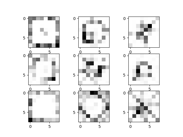
(a) LB-CDI, $N_{train}=1000$

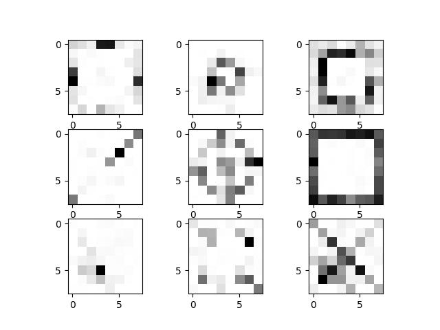
(b) SVI, $N_{train}=1000$

Figure 1: The recovered parameters after training with $1000$ data points using LB-CDI and SVI.

Additionally, we did the parameter estimation experiments on multi-mnist dataset. And the experiment results are depicted in Fig. 2. Here, since the training set of multi-mnist is large, we did not do LB-CDI.

In Fig. 2, similar phenomenon has been observed. When we have large amount of training data, both AVI and ACP (Fig. 2(a) and 2(b)) recovered parameters well. Even though AVI did not capture pattern $``1"$, it is indeed not trivial to separate pattern $``1"$ and $``7"$ in this dataset. However, SVI did not recover the parameters well.

When we reduce the amount of training data, the number of patterns detected by AVI decreased largely, as three weight patterns are recovered as $``0"$, which also indicates worse latent representation learning. However for ACP, although it messed up pattern $``4"$ and $``5"$, it recovered all other patterns, even with small amount of training data.

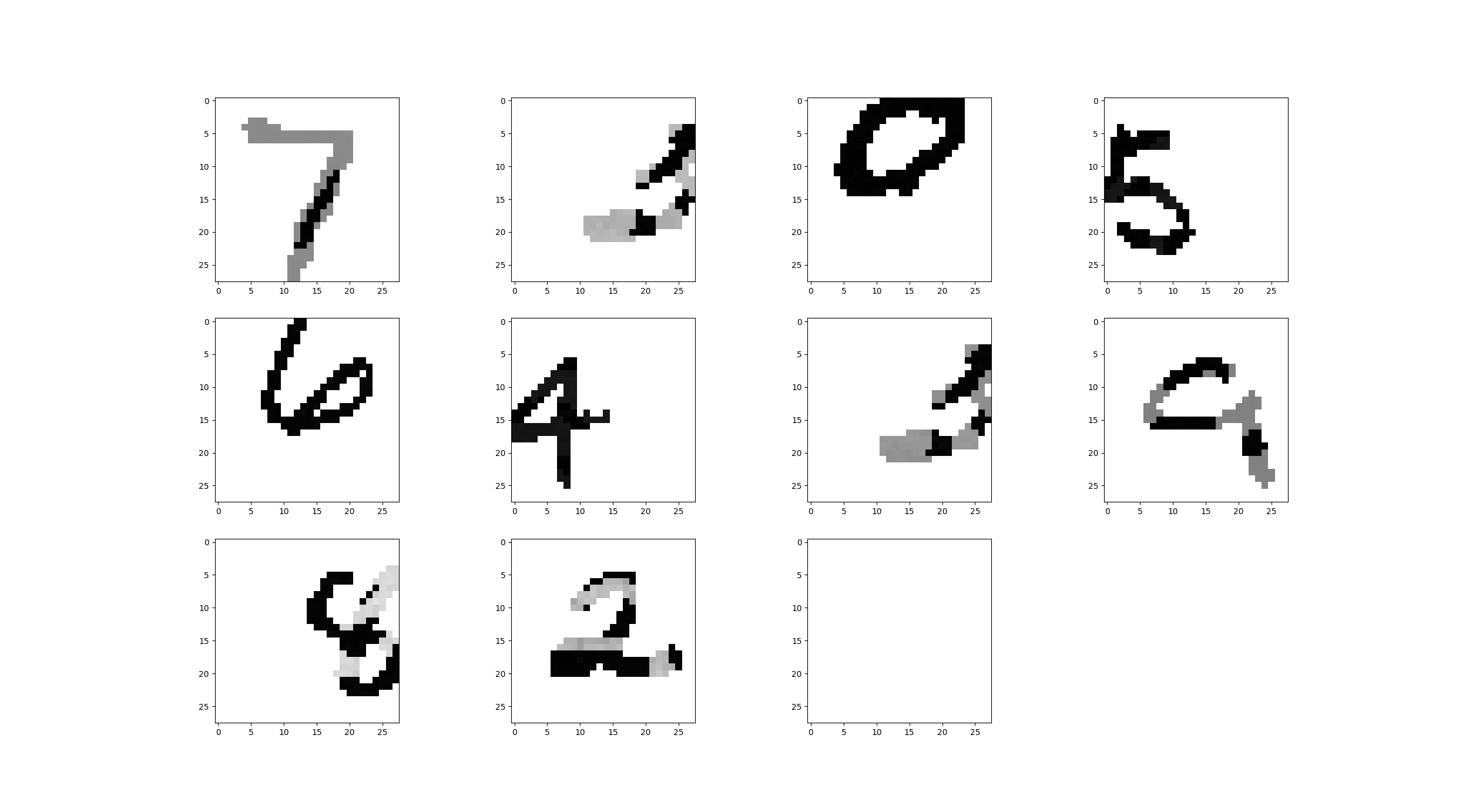
(a) AVI, $N_{train}=50K$

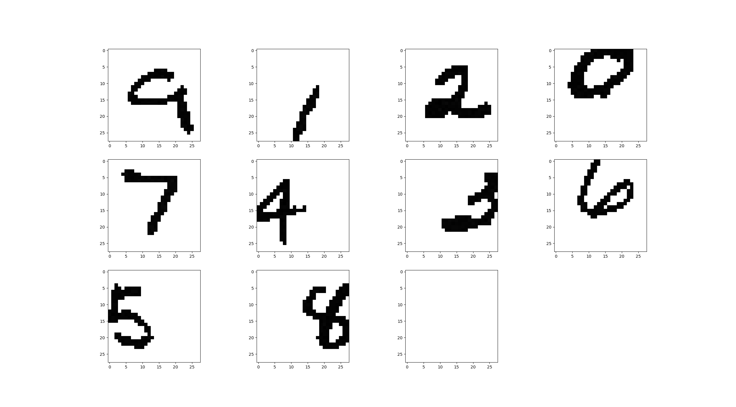
(b) ACP, $N_{train}=50K$

(c) AVI, $N_{train}=8K$

(d) ACP, $N_{train}=8K$

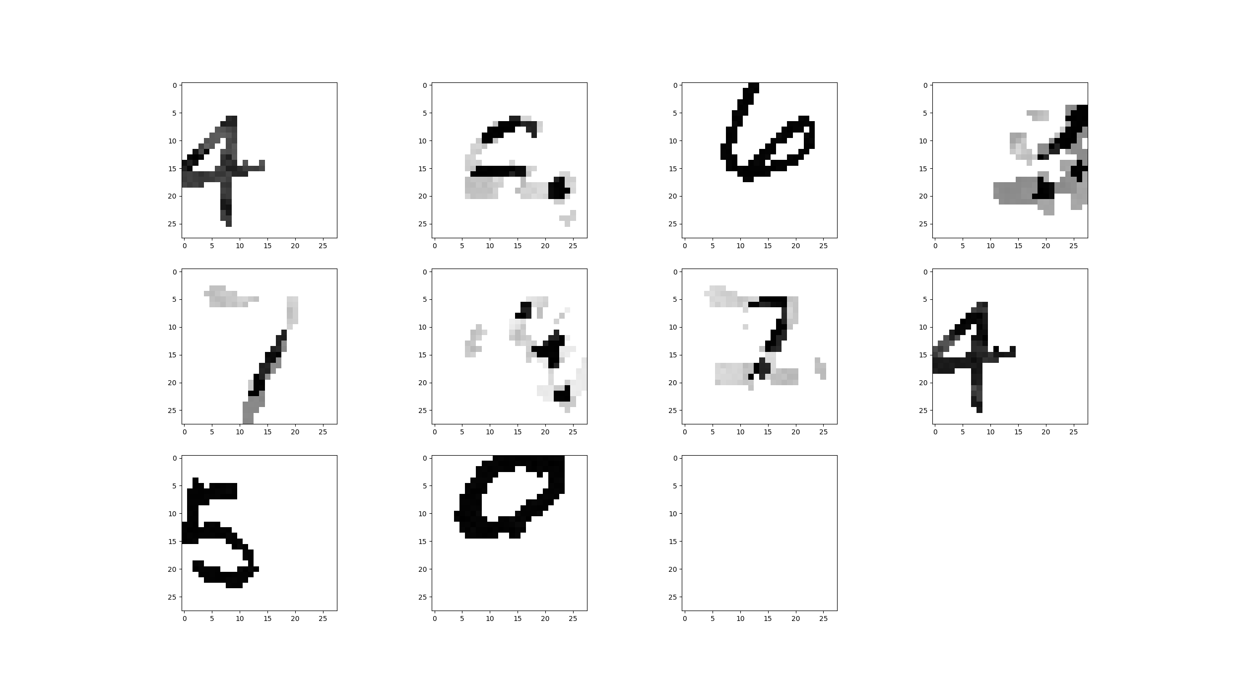
(e) SVI, $N_{train}=50K$

Figure 2: The recovered parameters of multi-mnist after training with $50K$ and $8K$ data points using AVI, ACP and SVI.

4 Additional experiments

4.1 Document classification

Herein, we aim to assess the impact of our inference method on noisy-or model’s learned representations. In particular, we rely on document classification task to evaluate the quality of the features learned by our model. To this end, we use the Reuters corpus from NLTK, which consists of $1.3$ million words and $10,788$ news articles organized into $90$ categories. For this experiment, we retain the top $3$ categories, namely acq, earn and money-fx. Each document is represented by its headline. We lemmatize the words, remove stop words, and remove words with less than $5$ occurrences. We obtain a final corpus of $839$ unique words and $7030$ documents, including $5048$ for training and $1982$ for test. Similar to topic modeling, each document is represented by a binary vector where each dimension indicates a word presence/absence.

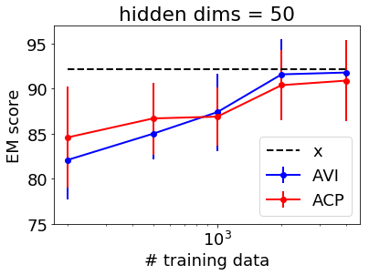
(a)

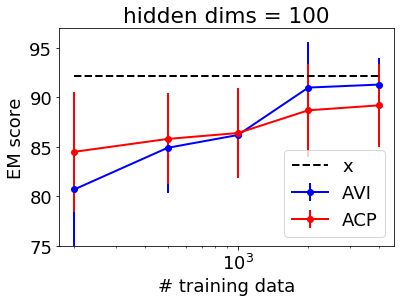
(b)

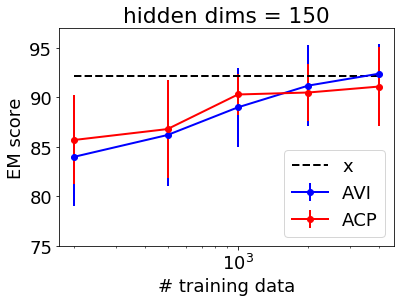
(c)

Figure 3: EM scores of AVI and ACP with different amount of training data and different hidden dimensions. The black dashed line indicates the classification performance with $\mathbf{x}$ in test set as input.

After training AVI and ACP, we take the approximate posterior distribution $\big{\{}q(z_{k}^{(n)}=1|\mathbf{x}^{(n);\bm{\phi}})\big{\}}_{k=1}^{K}$ as the latent representation of document $\mathbf{x}^{(n)}$. We evaluate the quality of learned representations on the test set. More specifically, we train a linear multilabel classifier, which takes the posterior distribution as input and predicts the document classes. We perform $5$-fold cross-validation and report the average EM scores.

Fig. 3 shows the classification performance with different amount of training data and different dimensionality of latent variables. The black dashed line corresponds to the results obtained when performing classification on the original space $\mathbf{X}$. We notice that when using a training set of more than $1000$ documents, AVI achieves higher classification accuracy owing to its larger inference capacity and flexibility. However, its performance drops quickly as we reduce the size of the training set. In contrast, our ACP inference offers more stability w.r.t. to the amount of training examples, and reaches higher classification performance when using smaller training sets.

We present in Fig. 4, 5 and 6 the t-SNE visualizations of the approximate posterior distributions learned by each model using 50, 100 and 150 hidden dimensions respectively. We observe that when using a small training set (middle and right columns), the acq and money-fx features learned by AVI tend to fuse together, while with ACP, we can still distinguish the three categories. This observation confirms our previous results and claims about the effectiveness of our model when lacking training data.

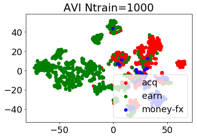
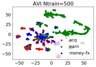
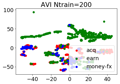
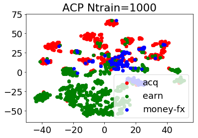
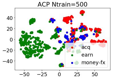
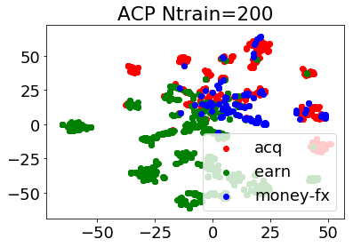
Figure 4: t-SNE visualization on latent representations on held out set when latent dimension is $50$.

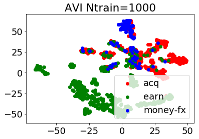
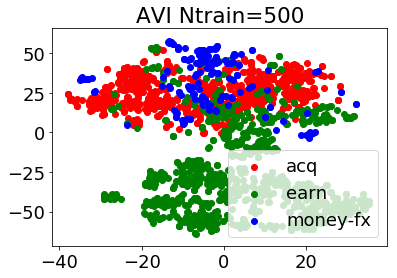
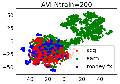
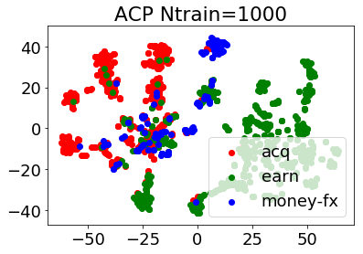
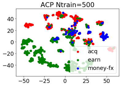
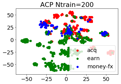
Figure 5: t-SNE visualization on latent representations on held out set when latent dimension is $100$.

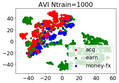
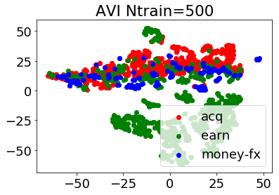
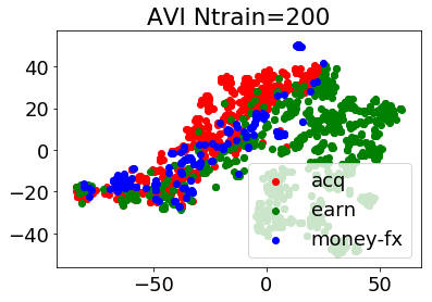
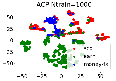
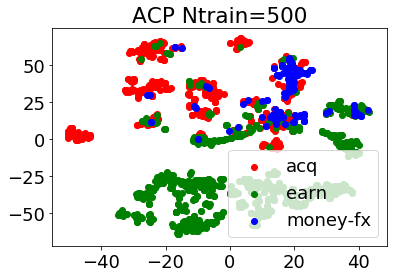
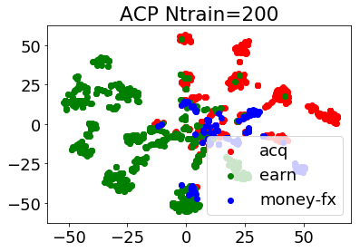
Figure 6: t-SNE visualization on latent representations on held out set when latent dimension is $150$.