Sparse Parallel Training of Hierarchical Dirichlet Process Topic Models

Abstract

To scale non-parametric extensions of probabilistic topic models such as Latent Dirichlet allocation to larger data sets, practitioners rely increasingly on parallel and distributed systems. In this work, we study data-parallel training for the hierarchical Dirichlet process (HDP) topic model. Based upon a representation of certain conditional distributions within an HDP, we propose a doubly sparse data-parallel sampler for the HDP topic model. This sampler utilizes all available sources of sparsity found in natural language—an important way to make computation efficient. We benchmark our method on a well-known corpus (PubMed) with 8m documents and 768m tokens, using a single multi-core machine in under four days.

1 Introduction

Topic models are a widely-used class of methods that allow practitioners to identify latent semantic themes in large bodies of text in an unsupervised manner. They are particularly attractive in areas such as history (Yang et al., 2011; Wang et al., 2012), sociology (DiMaggio et al., 2013), and political science (Roberts et al., 2014), where a desire for careful control of structure and prior information incorporated into the model motivates one to adopt a Bayesian approach to learning. In these areas, large corpora such as newspaper archives are becoming increasingly available (Ehrmann et al., 2020), and models such as latent Dirichlet allocation (LDA) (Blei et al., 2003) and its nonparametric extensions (Teh et al., 2006; Teh, 2006; Hu and Boyd-Graber, 2012; Paisley et al., 2015) are widely used by practitioners. Moreover, these models are emerging as a component of data-efficient language models (Guo et al., 2020). Training topic models efficiently entails two requirements.

1. Expose sufficient parallelism that can be taken advantage of by the hardware.

2. Utilize sparsity found in natural language to control memory requirements and computational complexity.

Symbol	Description		Symbol	Description
$V$	Vocabulary size		$\boldsymbol{\Psi}:1\times\infty$	Global distribution over topics
$D$	Total number of documents		$\mathbf{\Theta}:D\times\infty$	Document-topic probabilities
$N$	Total number of tokens		$\boldsymbol{\theta}_{d}:1\times\infty$	Topic probabilities for document $d$
$v(i)$	Word type for token $i$		$\mathbf{m}:D\times\infty$	Document-topic sufficient statistic
$d(i)$	Document for token $i$		$\mathbf{\Phi}:\infty\times V$	Topic-word probabilities
$w_{i,d}$	Token $i$ in document $d$		$\boldsymbol{\phi}_{k}:1\times V$	Word probabilities for topic $k$
$b_{i,d}$	Global topic draw indicator for $w_{i,d}$		$\mathbf{n}:\infty\times V$	Topic-word sufficient statistic
$z_{i,d}$	Topic indicator for token $i$ in $d$		$\boldsymbol{l}:1\times\infty$	Global topic latent sufficient statistic
$K^{*}$	Index for implicitly-represented topics		$\alpha,\boldsymbol{\beta},\gamma$	Prior concentration for $\boldsymbol{\theta}_{d}$, $\boldsymbol{\phi}_{k}$, $\boldsymbol{\Psi}$

Table 1: Notation for the HDP topic model. Sufficient statistics are conditional on the algorithm’s current iteration. Bold symbols refer to matrices, bold italics refer to vectors, possibly countably infinite.

In this work, we focus on the hierarchical Dirichlet process (HDP) topic model of Teh et al. (2006), which we review in Section 2. This model is a simple non-trivial extension of LDA to the nonparametric setting. This parallel implementation provides a blueprint for designing massively parallel training algorithms in more complicated settings, such as nonparametric dynamic topic models (Ahmed and Xing, 2010) and tree-based extensions (Hu and Boyd-Graber, 2012).

Parallel approaches to training HDPs have been previously introduced by a number of authors, including Newman et al. (2009), Wang et al. (2011), Williamson et al. (2013), Chang and Fisher (2014) and Ge et al. (2015). These techniques suit various settings: some are designed to explicitly incorporate sparsity present in natural language and other discrete spaces, while others are intended for HDP-based continuous mixture models. Gal and Ghahramani (2014) have pointed out that some methods can suffer from load-balancing issues, which limit their parallelism and scalability. The largest benchmark of parallel HDP training performed to our awareness is by Chang and Fisher (2014) on the 100m-token NYTimes corpora. Throughout this work, we focus on Markov chain Monte Carlo (MCMC) methods—empirically, their scalability is comparable to variational methods (Magnusson et al., 2018; Hoffman and Ma, 2019), and, subject to convergence, they yield the correct posterior.

Our contributions are as follows. We propose an augmented representation of the HDP for which the topic indicators can be sampled in parallel over documents. We prove that, under this representation, the global topic distribution $\boldsymbol{\Psi}$ is conditionally conjugate given an auxiliary parameter $\boldsymbol{l}$. We develop fast sampling schemes for $\boldsymbol{\Psi}$ and $\boldsymbol{l}$, and propose a training algorithm with a per-iteration complexity that depends on the minima of two sparsity terms—it takes advantage of both document-topic and topic-word sparsity simultaneously.

2 Partially collapsed Gibbs sampling for hierarchical Dirichlet processes

The hierarchical Dirichlet process topic model (Teh et al., 2006) begins with a global distribution $\boldsymbol{\Psi}$ over topics. Documents are assumed exchangeable—for each document $d$, the associated topic distribution $\boldsymbol{\theta}_{d}$ follows a Dirichlet process centered at $\boldsymbol{\Psi}$. Each topic is associated with a distribution of tokens $\boldsymbol{\phi}_{k}$. Within each document, tokens are assumed exchangeable (bag of words) and assigned to topic indicators $z_{i,d}$. For given data, we observe the tokens $w_{i,d}$.

We thus arrive at the GEM representation of a HDP, given by equation (19) of Teh et al. (2006) as

$$\boldsymbol{\Psi} \sim\operatorname{GEM}(\gamma)$$ (1)

$$\boldsymbol{\theta}_{d}\mid\boldsymbol{\Psi} \sim\operatorname{DP}(\alpha,\boldsymbol{\Psi})$$ (2)

$$\boldsymbol{\phi}_{k} \sim\operatorname{Dir}(\boldsymbol{\beta})$$ (3)

$$z_{i,d}\mid\boldsymbol{\theta}_{d} \sim\operatorname{Discrete}(\boldsymbol{\theta}_{d})$$ (4)

$$w_{i,d}\mid z_{i,d},\mathbf{\Phi} \sim\operatorname{Discrete}(\boldsymbol{\phi}_{z_{i,d}})$$ (5)

where $\alpha,\boldsymbol{\beta},\gamma$ are prior hyperparameters.

2.1 Intuition and augmented representation

At a high level, our strategy for constructing a scalable sampler is as follows. Conditional on $\boldsymbol{\Psi}$, the likelihood in equations (1)–(5) is the same as that of LDA. Using this observation, the Gibbs step for $\boldsymbol{z}$, which is the largest component of the model, can be handled efficiently by leveraging insights on sparse parallel sampling from the well-studied LDA literature (Yao et al., 2009; Li et al., 2014; Magnusson et al., 2018; Terenin et al., 2019). For this strategy to succeed, we need to ensure that all Gibbs steps involved in the HDP under this representation are analytically tractable and can be computed efficiently. For this, the representation needs to be modified.

To begin, we integrate each $\boldsymbol{\theta}_{d}$ out of the model, which by conjugacy (Blackwell and MacQueen, 1973) yields a Pólya sequence for each $\boldsymbol{z}_{d}$. By definition, given in Appendix A, this sequence is a mixture distribution with respect to a set of Bernoulli random variables $\boldsymbol{b}_{d}$, each representing whether $z_{i,d}$ was drawn from $\boldsymbol{\Psi}$ or from a repeated draw in the Pólya urn. Thus, the HDP can be written

$$\boldsymbol{\Psi} \sim\operatorname{GEM}(\gamma)$$ (6)

$$b_{i,d} \sim\operatorname{Ber}\big{(}{\textstyle\frac{\alpha}{i-1+\alpha}}\big{)}$$ (7)

$$\boldsymbol{\phi}_{k} \sim\operatorname{Dir}(\boldsymbol{\beta})$$ (8)

$$\boldsymbol{z}_{d}\mid\boldsymbol{b}_{d},\boldsymbol{\Psi} \sim\operatorname{PS}(\boldsymbol{\Psi},\boldsymbol{b}_{d})$$ (9)

$$w_{i,d}\mid z_{i,d} \sim\operatorname{Discrete}(\boldsymbol{\phi}_{z_{i,d}})$$ (10)

where $\operatorname{PS}(\boldsymbol{\Psi},\boldsymbol{b}_{d})$ is a Pólya sequence, defined in Appendix A. This representation defines a posterior distribution over $\boldsymbol{z},\mathbf{\Phi},\boldsymbol{\Psi},\boldsymbol{b}$ for the HDP. To derive a Gibbs sampler, we calculate its full conditionals.

2.2 Full conditionals for $\boldsymbol{z}$, $\mathbf{\Phi}$, and $\boldsymbol{b}$

The full conditionals $\boldsymbol{z}\mid\mathbf{\Phi},\boldsymbol{\Psi}$ and $\mathbf{\Phi}\mid\boldsymbol{z},\boldsymbol{\Psi}$, with $\boldsymbol{b}$ marginalized out, are essentially those in partially collapsed LDA (Magnusson et al., 2018; Terenin et al., 2019). They are

$$\operatorname{\mathbb{P}}(z_{i,d}=k \mid\boldsymbol{z}_{-i,d},\mathbf{\Phi},\boldsymbol{\Psi})$$ (11)

$$\propto\phi_{k,v(i)}\left[\alpha\Psi_{k}+m^{-i}_{d,k}\right]$$ (12)

where $v(i)$ is the word type for word token $i$, and

$$\boldsymbol{\phi}_{k}\mid\boldsymbol{z}\sim\operatorname{Dir}(\boldsymbol{\beta}+\boldsymbol{n}_{k})$$ (13)

where $m^{-i}_{d,k}$ denotes the document-topic sufficient statistic with index $i$ removed, and $\boldsymbol{n}_{k}$ is the topic-word sufficient statistic. Note the number of possible topics and full conditionals $\boldsymbol{\phi}_{k}\mid\boldsymbol{z}$ here is countably infinite. The full conditional for each $b_{i,d}$ is

$$\operatorname{\mathbb{P}}(b_{i,d}=1 \mid\boldsymbol{z}_{d},\boldsymbol{\Psi},\boldsymbol{b}_{-i,d})$$ (14)

$$=\frac{\alpha\Psi_{z_{i,d}}}{\alpha\Psi_{z_{i,d}}+\sum_{j=1}^{i}\mathbbold{1}_{z_{j,d}}(z_{i,d})}.$$ (15)

The derivation, based on a direct application of Bayes’ Rule with respect to the probability mass function of the Pólya sequence, is in Appendix A.

2.3 The full conditional for $\mathbf{\Psi}$

To derive the full conditional for $\boldsymbol{\Psi}$, we examine the prior and likelihood components of the model. It is shown in Appendix A that the likelihood term $\boldsymbol{z}_{d}\mid\boldsymbol{b}_{d},\boldsymbol{\Psi}$ may be written

$$p (\boldsymbol{z}_{d}\mid\boldsymbol{b}_{d},\boldsymbol{\Psi})$$ (16)

$$=\underbracket{\prod_{\begin{subarray}{c}i=1\\ b_{i,d}\neq 1\end{subarray}}^{N_{d}}\sum_{j=1}^{i-1}\frac{1}{i-1}\mathbbold{1}_{z_{j,d}}(z_{i,d})}_{\smash{\mathrel{\text{missing}}{doesn^{\prime}tenterposterior}}}\prod_{\begin{subarray}{c}i=1\\ b_{i,d}=1\end{subarray}}^{N_{d}}\prod_{k=1}^{\infty}\Psi_{k}^{\mathbbold{1}_{k}(z_{i,d})}.$$

The first term is a multiplicative constant independent of $\boldsymbol{\Psi}$ and vanishes via normalization. Thus, the full conditional $\boldsymbol{\Psi}\mid\boldsymbol{z},\boldsymbol{b}$ depends on $\boldsymbol{z}$ and $\boldsymbol{b}$ only through the sufficient statistic $\boldsymbol{l}$ defined by

$$l_{k}=\sum_{d=1}^{D}\sum_{\begin{subarray}{c}i=1\\ \smash{b_{i,d}=1}\end{subarray}}^{N_{d}}\mathbbold{1}_{z_{i,d}=k}$$ (17)

and so we may suppose without loss of generality that the likelihood term is categorical. Under these conditions, we prove the full conditional for $\boldsymbol{\Psi}$ admits a stick-breaking representation.

Proposition 1.

Without loss of generality, suppose

$$\boldsymbol{\Psi} \sim\operatorname{GEM}(\gamma) \boldsymbol{x}\mid\boldsymbol{\Psi} \sim\operatorname{Discrete}(\boldsymbol{\Psi}).$$ (18)

Then $\boldsymbol{\Psi}\mid\boldsymbol{x}$ is given by

$$\!\!\!\!\Psi_{k}=\varsigma_{k}\prod_{i=1}^{k-1}(1-\varsigma_{i})\quad\varsigma_{k}\sim\operatorname{Beta}(a^{(\boldsymbol{\Psi})}_{k}\!,b^{(\boldsymbol{\Psi})}_{k})\!\!\!$$ (19)

$$a^{(\boldsymbol{\Psi})}_{k}=1+l_{k}\,\,\quad\,\,b^{(\boldsymbol{\Psi})}_{k}=\gamma+\sum_{i=k+1}^{\smash{\infty}}l_{i}$$ (20)

where $\boldsymbol{l}$ are the empirical counts of $\boldsymbol{x}$.

Proof.

Appendix B. ∎

This expression is similar to the stick-breaking representation of a Dirichlet process $\operatorname{DP}(\cdot,F)$—however, it has different weights and does not include random atoms drawn from $F$ as part of its definition—see Appendix B for more details. Putting these ideas together, we define an infinite-dimensional parallel Gibbs sampler.

Algorithm 1.

Repeat until convergence.

• Sample $\boldsymbol{\phi}_{k}\sim\operatorname{Dir}(\boldsymbol{n}_{k}+\boldsymbol{\beta})$ in parallel over topics for $k=1,..,\infty$.

• Sample $z_{i,d}\propto\phi_{k,v(i)}\,\alpha\,\Psi_{k}+\phi_{k,v(i)}\,m_{d,k}^{-i}$ in parallel over documents for $d=1,..,D$.

• Sample $b_{i,d}$ according to equation (14) in parallel over documents for $d=1,..,D$.

• Sample $\boldsymbol{\Psi}$ according to equations (19)–(20).

Algorithm 1 is completely parallel, but cannot be implemented as stated due to the infinite number of full conditionals for $\mathbf{\Phi}$, as well as the infinite product used in sampling $\boldsymbol{\Psi}$. We now bypass these issues by introducing an approximate finite-dimensional sampling scheme.

2.4 Finite-dimensional sampling of $\mathbf{\Psi}$ and $\mathbf{\Phi}$

By way of assuming $\boldsymbol{\Psi}\sim\operatorname{GEM}(\gamma)$, an HDP assumes an infinite number of topics are present a priori, with the number of tokens per topic decreasing rapidly with the topic’s index in a manner controlled by $\gamma$. Thus, under the model, a topic with a sufficiently large index should contain no tokens with high probability.

We thus propose to approximate $\boldsymbol{\Psi}$ by projecting its tail onto a single flag topic $K^{*}$, which stands for all topics not explicitly represented as part of the computation. This can be done by by deterministically setting $\varsigma_{K^{*}}=1$ in equation (19). The resulting finite-dimensional $\boldsymbol{\Psi}$ will be the correct posterior full conditional for the finite-dimensional generalized Dirichlet prior considered previously in Section 2.3. Hence, this finite-dimensional truncation forms a Bayesian model in its own right, which suggests it should perform reasonably well. From an asymptotic perspective, Ishwaran and James (2001) have shown that the approximation is almost surely convergent and, therefore, well-posed.

Once this is done, $\boldsymbol{\Psi}$ becomes a finite vector of length $K^{*}$, and only $K^{*}$ rows of $\mathbf{\Phi}$ need to be explicitly instantiated as part of the computation. This instantiation allows the algorithm to be defined on a fixed finite state space, simplifying bookkeeping and implementation.

From a computational efficiency perspective, the resulting value $K^{*}$ takes the place of $K$ in partially collapsed LDA. However, it cannot be interpreted as the number of topics in the sense of LDA. Indeed, LDA implicitly assumes that $\boldsymbol{\Psi}=\operatorname{Unif}(1,..,K)$ deterministically—i.e., that every topic is assumed a priori to contain the same number of tokens. In contrast, the HDP model learns this distribution from the data by letting $\boldsymbol{\Psi}\sim\operatorname{GEM}(\gamma)$.

If we allow the state space to be resized when topic $K^{*}$ is sampled, then following Papaspiliopoulos and Roberts (2008), it is possible to develop truncation schemes which introduce no error. Since this results in more complicated bookkeeping which reduces performance, we instead fix $K^{*}$ and defer such considerations to future work. We recommend setting $K^{*}$ to be sufficiently large that it does not significantly affect the model’s behavior, which can be checked by tracking the number of tokens assigned to the topic $K^{*}$.

2.5 Sparse sampling of $\mathbf{\Phi}$ and $\boldsymbol{z}$

To be efficient, a topic model needs to utilize the sparsity found in natural language as much as possible. In our case, the two main sources of sparsity are as follows.

1. Document-topic sparsity: most documents will only contain a handful of topics.

2. Topic-word sparsity: most word types will not be present in most topics.

We thus expect the document-topic sufficient statistic $\mathbf{m}$ and topic-word sufficient statistic $\mathbf{n}$ to contain many zeros. We seek to use this to reduce sampling complexity. Our starting point is the Poisson Pólya Urn sampler of Terenin et al. (2019), which presents a Gibbs sampler for LDA with computational complexity that depends on the minima of two sparsity coefficients representing document-topic and topic-word sparsity—such algorithms are termed doubly sparse. The key idea is to approximate the Dirichlet full conditional for $\boldsymbol{\phi}_{k}$ with a Poisson Pólya Urn (PPU) distribution defined by

$$\!\!\!\phi_{k,v} \!=\!\frac{\varphi_{k,v}}{\sum_{v=1}^{V}\varphi_{k,v}} \varphi_{k,v} \!\sim\!\operatorname{Pois}(\beta_{k,v}\!+\!n_{k,v})$$ (21)

for $v=1,..,V$. This distribution is discrete, so $\mathbf{\Phi}$ becomes a sparse matrix. The approximation is accurate even for small values of $n_{k,v}$, and Terenin et al. (2019) proves that the approximation error will vanish for large data sets in the sense of convergence in distribution.

If $\boldsymbol{\beta}$ is uniform, we can further use sparsity to accelerate sampling $\varphi_{k,v}$. Since a sum of Poisson random variables is Poisson, we can split $\varphi_{k,v}=\varphi_{k,v}^{\smash{(\beta)}}+\varphi_{k,v}^{\smash{(\mathbf{n})}}$. We then sample $\varphi_{k,v}^{\smash{(\beta)}}$ sparsely by introducing a Poisson process and sampling its points uniformly, and sample $\varphi_{k,v}^{\smash{(\mathbf{n})}}$ sparsely by iterating over nonzero entries of $\mathbf{n}$.

  See http://mallet.cs.umass.edu and https://github.com/lejon/PartiallyCollapsedLDA. AP and CGCBIB can be found therein. NeurIPS and PubMed can be found at https://archive.ics.uci.edu/ml/datasets/bag+of+words. Full output of experiments can be found at https://github.com/aterenin/Parallel-HDP-Experiments/.

For $\boldsymbol{z}$, the full conditional

$$\operatorname{\mathbb{P}}(z_{i,d}=k \mid\boldsymbol{z}_{-i,d},\mathbf{\Phi},\boldsymbol{\Psi})$$ (22)

$$\propto\phi_{k,v(i)}\left[\alpha\Psi_{k}+m^{-i}_{d,k}\right]$$ (23)

$$\propto\underbracket{\phi_{k,v(i)}\alpha\Psi_{k}\vphantom{\phi_{k,v(i)}m^{-i}_{d,k}}}_{(a)\vphantom{(b)}}+\underbracket{\phi_{k,v(i)}m^{-i}_{d,k}\vphantom{\phi_{k,v(i)}\alpha\Psi_{k}}}_{(b)\vphantom{(a)}}$$ (24)

is similar to to the one in partially collapsed LDA (Magnusson et al., 2018)—the difference is the presence of $\Psi_{k}$. As $\Psi_{k}$ only enters the expression through component $(a)$ and is identical for all $z_{i,d}$, it can be absorbed at each iteration directly into an alias table (Walker, 1977; Li et al., 2014). Component $(b)$ can be computed efficiently by utilizing sparsity of $\mathbf{\Phi}$ and $\mathbf{m}$ and iterating over whichever has fewer non-zero entries.

2.6 Direct sampling of $\boldsymbol{l}$

Rather than sampling $\boldsymbol{b}$, whose size will grow linearly with the number of documents, we introduce a scheme for sampling the sufficient statistic $\boldsymbol{l}$ directly. Observe that

$$l_{k}=\sum_{d=1}^{D}\sum_{\begin{subarray}{c}i=1\\ b_{i,d}=1\end{subarray}}^{N_{d}}\mathbbold{1}_{z_{n,d}=k}=\sum_{d=1}^{D}\sum_{\begin{subarray}{c}i=1\\ z_{i,d}=k\end{subarray}}^{N_{d}}\mathbbold{1}_{b_{i,d}=1}$$ (25)

where the domain of summation and the value of the indicators have been switched. By definition of $b_{i,d}$, we have

$$\sum_{\begin{subarray}{c}i=1\\ z_{i,d}=k\end{subarray}}^{N_{d}}\mathbbold{1}_{b_{i,d}=1}=\sum_{j=1}^{m_{d,k}}b_{j,d,k}$$ (26)

where

$$b_{j,d,k}\sim\operatorname{Ber}\left(\frac{\Psi_{k}\alpha}{\Psi_{k}\alpha+j-1}\right).$$ (27)

Summing this expression over documents, we obtain the expression

$$\!\!\!l_{k} \!=\!\sum_{j=1}^{\mathclap{\max_{d}m_{d,k}}}c_{j,k} c_{j,k} \!\sim\!\operatorname{Bin}\left(\!D_{k,j},\frac{\Psi_{k}\alpha}{\Psi_{k}\alpha\!+\!j\!-\!1}\!\right)\!\!$$ (28)

where $D_{k,j}$ is the total number of documents with $m_{d,k}\geq j$. Since $m_{d,k}=0$ for all topics $k$ without any tokens assigned, we only need to sample $\boldsymbol{l}$ for topics that have tokens assigned to them. This idea can also be straightforwardly applied to other HDP samplers (Chang and Fisher, 2014; Ge et al., 2015), by allowing one to derive alternative full conditionals in lieu of the Stirling distribution (Antoniak, 1974). The complexity of sampling $\boldsymbol{l}$ directly is constant with respect to the number of documents, and depends instead on the maximum number of tokens per document.

To handle the bookkeeping necessary for computing $D_{k,j}$, we introduce a sparse matrix $\mathbf{d}$ of size $K\times\max_{d}N_{d}$ whose entries $d_{k,p}$ are the number of documents for topic $k$ that have a total of $p$ topic indicators assigned to them. We increment $\mathbf{d}$ once $\boldsymbol{z}_{d}$ been sampled by iterating over non-zero elements in $\boldsymbol{m}_{d}$. We then compute $D_{k,j}$ as the reverse cumulative sum of the rows of $\mathbf{d}$.

2.7 Poisson Pólya urn partially collapsed Gibbs sampling

Putting all of these ideas together, we obtain the following algorithm.

Algorithm 2.

Repeat until convergence.

• Sample $\boldsymbol{\phi}_{k}\sim\operatorname{PPU}(\boldsymbol{n}_{k}+\boldsymbol{\beta})$ in parallel over topics for $k=1,..,K^{*}$.

• Sample $z_{i,d}\propto\phi_{k,v(i)}\,\alpha\,\Psi_{k}+\phi_{k,v(i)}\,m_{d,k}^{-i}$ in parallel over documents for $d=1,..,D$.

• Sample $l_{k}$ according to equation (28) in parallel over topics for $k=1,..,K^{*}$.

• Sample $\boldsymbol{\Psi}$ according to equations (19)–(20), except with $\varsigma_{K^{*}}=1$.

Algorithm 2 is sparse, massively parallel, defined on a fixed finite state space, and contains no infinite computations in any of its steps. The Gibbs step for $\mathbf{\Phi}$ converges in distribution (Terenin et al., 2019) to the true Gibbs steps as $N\rightarrow\infty$, and the Gibbs step for $\boldsymbol{\Psi}$ converges almost surely (Ishwaran and James, 2001) to the true Gibbs step as $K^{*}\rightarrow\infty$.

2.8 Computational complexity

We now examine the per-iteration computational complexity of Algorithm 2. To proceed, we fix $K^{*}$ and maximum document size $\max_{d}N_{d}$, and relate the vocabulary size $V$ with the number $N$ of total words as follows.

Assumption (Heaps’ Law).

The number of unique words in a corpus follows Heaps’ law (Heaps, 1978) $V=\xi N^{\zeta}$ with constants $\xi>0$ and $\zeta<1$.

The per-iteration complexity of Algorithm 2 is equal to the sum of the per-iteration complexity of sampling its components. The sampling complexities of $\boldsymbol{\Psi}$ and $\boldsymbol{l}$ are constant with respect to the number of tokens, and the sampling complexity of $\mathbf{\Phi}$ has been shown by Magnusson et al. (2018) to be negligible under the given assumptions. Thus, it suffices to consider $\boldsymbol{z}$.

At a given iteration, let $\smash{K_{d(i)}^{(\mathbf{m})}}$ be the number of existing topics in document $d$ associated with word token $i$, and let $\smash{K^{(\mathbf{\Phi})}_{v(i)}}$ be the number of nonzero topics in the row of $\mathbf{\Phi}$ corresponding to word token $i$. It follows immediately from the argument given by Terenin et al. (2019) that the per-iteration complexity of sampling each topic indicator $z_{i}$ is

$$\mathcal{O}\left[\min\left(K^{(\mathbf{m})}_{d(i)},K^{(\mathbf{\Phi})}_{v(i)}\right)\right].$$ (29)

Algorithm 2 is thus a doubly sparse algorithm.

Corpus	$V$	$D$	$N$		Iterations	Threads	Runtime
AP	7 074	2 206	393 567		100 000	8	3.8 hours
CGCBIB	6 079	5 940	570 370		100 000	12	2.7 hours
NeurIPS	12 419	1 499	1 894 051		255 500	8	24 hours
PubMed	89 987	8 199 999	768 434 972		25 000	20	82.4 hours

Table 2: Corpora used in experiments, together with compute configuration.

3 Performance results

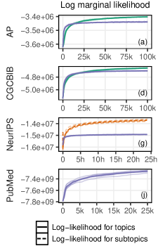
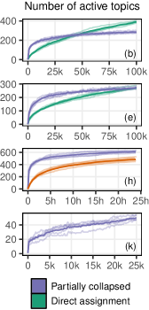
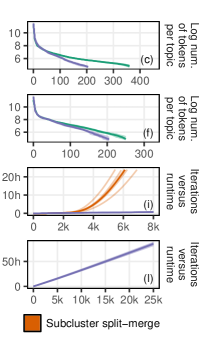
Figure 1: Trace plots for log-likelihood, number of active topics, and additional metrics for CGCBIB, NeurIPS, and PubMed. On the $x$ axis, per-iteration scale is used for AP, CGCBIB and PubMed, and real-time scale is used for NeurIPS. Algorithms used are partially collapsed HDP for all corpora, direct assignment HDP for AP and CGCBIB, and subcluster split-merge HDP for NeurIPS. Individual traces are partially transparent, and their mean is opaque.

To study performance of the partially collapsed sampler—Algorithm 2—we implemented it in Java using the open-source Mallet (McCallum, 2002) topic modeling framework. We ran it on the AP, CGCBIB, NeurIPS, and PubMed corpora, which are summarized in Table 2. Prior hyperparameters controlling the degree of sparsity were set to $\alpha=0.1,\beta=0.01,\gamma=1$. We set $K^{*}=1000$ and observed no tokens ever allocated to the topic $K^{*}$. Data were preprocessed with default Mallet (McCallum, 2002) stop-word removal, minimum document size of 10, and a rare word limit of 10. Following Teh et al. (2006), the algorithm was initialized with one topic. All experiments were repeated five times to assess variability. Total runtime for each experiment is given in Table 2.

To assess Algorithm 2 in a small-scale setting, we compare it to the widely-studied sparse fully collapsed direct assignment sampler of Teh et al. (2006), which is not parallel. We ran 100 000 iterations of both methods on AP and CGCBIB. We selected these corpora because they were among the larger corpora on which it was feasible to run our direct assignment reference implementation within one week.

Trace plots for the log marginal likelihood for $\boldsymbol{z}$ given $\boldsymbol{\Psi}$ and the number of active topics, i.e., those topics assigned at least one token, can be seen in Figure 1(a,d) and Figure 1(b,e), respectively. The direct assignment algorithm converges slower, but achieves a slightly better local optimum in terms of marginal log-likelihood, compared to our method. This fact indicates that the direct assignment method may stabilize around a different local optimum, and may represent a potential limitation of the partially collapsed sampler in settings where non-parallel methods are practical.

To better understand the distributional differences between the algorithms, we examined the number of tokens per topic, which can be seen in Figure 1(c,f). The partially collapsed sampler is seen to assign more tokens to smaller topics, indicating that it stabilizes around a local optimum with slightly broader semantic themes.

To visualize the effect this has on the topics, we examined the most common words for each topic. Since the algorithms generate too many topics to make full examination practical, we instead compute a quantile summary with five topics per quantile. The quantile is computed by ranking all topics by the number of tokens, choosing the five closest topics to the $100\%$, $75\%$, $50\%$, $25\%$, and $5\%$ quantiles in the ranking, and computing their top words. This approach gives a representative view of the algorithm’s output for large, medium, and small topics. Results may be seen in Appendix D and Appendix C—we find the direct assignment and partially collapsed samplers to be mostly comparable, with substantial overlap in top words for common topics.

Next, we assess Algorithm 2 in a more demanding setting and compare against previous parallel state-of-the-art. There are various scalable samplers available for the HDP. For a fair comparison, we restrict ourselves to those samplers designed for topic models and explicitly incorporate sparsity of natural language in their construction. Among these, we selected the parallel subcluster split-merge algorithm of Chang and Fisher (2014) as our baseline because it was used in the largest-scale benchmark of the HDP topic model performed to date to our awareness, and shows comparable performance to other methods (Ge et al., 2015). The subcluster split-merge algorithm is designed to converge with fewer iterations, but is more costly to run per iteration. Thus, we used a fixed computational budget of 24 hours of wall-clock time for both algorithms. Computation was performed on a system with a 4-core 8-thread CPU and 8GB RAM.

Results can be seen in Figure 1(g)—note that the subcluster split-merge algorithm is parametrized using sub-topic indicators and sub-topic probabilities, so its numerical log-likelihood values are not directly comparable to ours and should be interpreted purely to assess convergence. Algorithm 2 stabilizes much faster with respect to both the number of active topics in Figure 1(g), and marginal log-likelihood in Figure 1(h). The subcluster split-merge algorithm adds new topics one-at-a-time, whereas our algorithm can create multiple new topics per iteration—we hypothesize this difference leads to faster convergence for Algorithm 2.

In Figure 1(i), we observe that the amount of computing time per iteration increases substantially for the subcluster split-merge method as it adds more topics. For Algorithm 2, this stays approximately constant for its entire runtime.

To evaluate the topics produced by the algorithms, we again examined the most common words for each topic via a quantile summary, given in Appendix E. We find the subcluster split-merge algorithm appears to generate topics with slightly more semantic overlap compared to Algorithm 2, but otherwise produces comparable output.

Finally, to assess scalability, we ran 25 000 iterations of Algorithm 2 on PubMed, which contains 768m tokens. To our knowledge, this dataset is an order of magnitude larger than any datasets used in previous MCMC-based approaches for the HDP. Computation was performed on a compute node with 2x10-core CPUs with 20 threads and 64GB of RAM. The marginal likelihood and number of active topics are given in Figure 1(j) and Figure 1(k).

To evaluate the topics discovered by the algorithm, we examined their most common words—these may be seen in full in Appendix F. We observe that the semantic themes present in the topics vary according to how many tokens they have: topics with more tokens appear to be broader, whereas topics with fewer tokens appear to be more specific. This behavior illustrates a key difference between the HDP and methods like LDA, which do not contain a learned global topic distribution $\boldsymbol{\Psi}$ in their formulation. We suspect the effect is particularly pronounced on PubMed compared to CGCBIB and NeurIPS due to its large number of tokens.

$k$	Topic 1	Topic 5	Topic 9	Topic 13	Topic 17
$n_{k,\mathbin{\vbox{\hbox{\scalebox{0.5}{$\bullet$}}}}}$	42 395 289	23 907 517	22 167 377	20 925 933	18 924 590
	care	cancer	protein	protein	cell
	health	tumor	binding	cell	neuron
	patient	patient	membrane	kinase	electron
	medical	cell	acid	expression	brain
	research	carcinoma	activity	receptor	rat
	system	breast	cell	activation	nerve
	clinical	tumour	gel	pathway	fiber
	cost	survival	human	phosphorylati	nucleus

$k$	Topic 21	Topic 25	Topic 29	Topic 33	Topic 37
$n_{k,\mathbin{\vbox{\hbox{\scalebox{0.5}{$\bullet$}}}}}$	18 033 777	16 308 024	15 128 822	13 562 338	10 819 160
	cell	rat	gene	infection	plant
	growth	day	mutation	strain	strain
	expression	mice	genetic	antibiotic	acid
	factor	liver	chromosome	bacterial	growth
	beta	animal	analysis	isolates	extract
	human	effect	genes	bacteria	activity
	mrna	control	polymorphism	resistance	cell
	endothelial	mg	dna	coli	production

Figure 2: Top 8 words for topics obtained by Algorithm 2 on PubMed, together with topic index $k$ and total number of words $n_{k,\mathbin{\vbox{\hbox{\scalebox{0.5}{$\bullet$}}}}}$ present in the topic. We observe that the topics range from broad to specific: this is a consequence of the hierarchical Dirichlet process prior via the inclusion of the global topic proportions $\boldsymbol{\Psi}$. Topics obtained by Algorithm 2 on all corpora may be seen in Appendix C, Appendix D, Appendix E, and Appendix F.

4 Discussion

In this work, we introduce the parallel partially collapsed Gibbs sampler—Algorithm 1—for the HDP topic model, which converges to the correct target distribution. We propose a doubly sparse approximate sampler—Algorithm 2—which allows the HDP to be implemented with per-token sampling complexity of $\smash{\mathcal{O}\big{[}\min\big{(}K^{(\mathbf{m})}_{d(i)},K^{(\mathbf{\Phi})}_{v(i)}\big{)}\big{]}}$ which is the same as that of Pólya Urn LDA (Terenin et al., 2019). Compared to other approaches for the HDP, it offers the following improvements.

1. The algorithm is fully parallel in all steps.

2. The topic indicators $\boldsymbol{z}$ utilize all available sources of sparsity to accelerate sampling.

3. All steps not involving $\boldsymbol{z}$ have constant complexity with respect to data size.

4. The proposed sparse approximate algorithm becomes exact as $N\rightarrow\infty$ and $K^{*}\rightarrow\infty$.

These improvements allow us to train the HDP on larger corpora. The data-parallel nature of our approach means that the amount of available parallelism increases with data size. This parallelism avoids load-balancing-related scalability limitations pointed out by Gal and Ghahramani (2014).

Nonparametric topic models are less straightforward to evaluate empirically than ordinary topic models. In particular, we found topic coherence scores (Mimno et al., 2011) to be strongly affected by the number of active topics $K$, which causes preference for models with fewer topics and more semantic overlap per topic. We view the development of summary statistics that are $K$-agnostic and those measuring other aspects of topic quality such as overlap, to be an important direction for future work. We are particularly interested in techniques that can be used to compare algorithms for sampling from the same model defined over fully disjoint state spaces, such as Algorithm 2 and the subcluster split-merge algorithm in Section 3.

Partially collapsed HDP can stabilize around a different local mode than fully collapsed HDP as proposed by Teh et al. (2006). There have been attempts to improve mixing in that sampler (Chang and Fisher, 2014), including the use of Metropolis-Hastings steps for jumping between modes (Jain and Neal, 2004). These techniques are largely complementary to ours and can be explored in combination with the ideas presented here.

The HDP posterior is a heavily multimodal target for which full posterior exploration is known to be difficult (Chang and Fisher, 2014; Gal and Ghahramani, 2014; Buntine and Mishra, 2014), and sampling schemes are generally used more in the spirit of optimization than traditional MCMC. These issues are mirrored in other approaches, such as variational inference. There, restrictive mean-field factorization assumptions are often required, which reduces the quality of discovered topics. We view MAP-based analogs of ideas presented here as a promising direction, since these may allow additional flexibility that may enable faster training.

Many of the ideas in this work, such as the binomial trick, are generic and apply to any topic model structurally similar to the HDP’s GEM representation (Teh et al., 2006) given in Section 2. For example, one could consider an informative prior for $\boldsymbol{\Psi}$ in lieu of $\operatorname{GEM}(\gamma)$, potentially improving convergence and topic quality, or developing parallel schemes for other nonparametric topic models such as Pitman-Yor models (Teh, 2006), tree-based models (Hu and Boyd-Graber, 2012; Paisley et al., 2015), embedded topic models (Dieng et al., 2020), as well as nonparametric topic models used within data-efficient language models (Guo et al., 2020) in future work.

Conclusion

We introduce the doubly sparse partially collapsed Gibbs sampler for the hierarchical Dirichlet process topic model. By formulating this algorithm using a representation of the HDP which connects it with the well-studied Latent Dirichlet Allocation model, we obtain a parallel algorithm whose per-token sampling complexity is the minima of two sparsity terms. The ideas used apply to a large array of topic models, for example, dynamic topic models with $\mathbf{\Phi}$ time-varying, which possess the same full conditional for $\boldsymbol{z}$. Our algorithm for the HDP scales to a 768m-token corpus (PubMed) on a single multicore machine in under four days.

The proposed techniques leverage parallelism and sparsity to scale nonparametric topic models to larger datasets than previously considered feasible for MCMC or other methods possessing similar convergence properties. We hope these contributions enable wider use of Bayesian nonparametrics for large collections of text.

Acknowledgments

The research was funded by the Academy of Finland (grants 298742, 313122), as well as the Swedish Research Council (grants 201805170, 201806063). Computations were performed using compute resources within the Aalto University School of Science and Department of Computing at Imperial College London. We also acknowledge the support of Ericsson AB.

Appendix A Appendix: sufficiency of $\boldsymbol{l}$ and full conditional for $\boldsymbol{b}$

Recall that the one-step-ahead conditional probability mass function in a Pólya sequence taking values in $\mathbb{N}$ with concentration parameter $\alpha$ and base probability mass function $\boldsymbol{\Psi}$ is

$$p(z_{i}\mid z_{i-1},..,z_{1},\boldsymbol{\Psi})=\sum_{j=1}^{i-1}\frac{1}{i-1+\alpha}\mathbbold{1}_{z_{j}}(z_{i})+\frac{\alpha}{i-1+\alpha}\Psi_{z_{i}}.$$ (30)

Introducing the random variable

$$b_{i}\sim\operatorname{Ber}\left(\frac{\alpha}{i-1+\alpha}\right)$$ (31)

we can express the one-step-ahead conditional distribution as

$$p(z_{i}\mid z_{i-1},..,z_{1},b_{i},\boldsymbol{\Psi})=\mathbbold{1}_{b_{i}=0}\sum_{j=1}^{i-1}\frac{1}{i-1}\mathbbold{1}_{z_{j}}(z_{i})+\mathbbold{1}_{b_{i}=1}\Psi_{z_{i}}.$$ (32)

The joint probability mass function for $\boldsymbol{z}\mid\boldsymbol{b},\boldsymbol{\Psi}$ is then

$$p(\boldsymbol{z}\mid\boldsymbol{b},\boldsymbol{\Psi})=\prod_{i=1}^{N}p(z_{i}\mid z_{i-1},..,z_{1},\boldsymbol{b},\boldsymbol{\Psi})=\prod_{i=1}^{N}\left[\sum_{j=1}^{i-1}\mathbbold{1}_{b_{i}=0}\mathbbold{1}_{z_{j}}(z_{i})+\mathbbold{1}_{b_{i}=1}\Psi_{z_{i}}\right].$$ (33)

Note that $\mathbbold{1}_{b_{i}=0}=1\iff\mathbbold{1}_{b_{i}=1}=0$ and vice versa. Thus each term in the product for $\boldsymbol{z}\mid\boldsymbol{b},\boldsymbol{\Psi}$ only has one component, and we may express $\boldsymbol{z}\mid\boldsymbol{b},\boldsymbol{\Psi}$ as

$$p(\boldsymbol{z}\mid\boldsymbol{b},\boldsymbol{\Psi})=\underbracket{\prod_{\begin{subarray}{c}i=1\\ b_{i}\neq 1\end{subarray}}^{N}\sum_{j=1}^{i-1}\frac{1}{i-1}\mathbbold{1}_{z_{j}}(z_{i})}_{\mathrel{\text{missing}}{doesn^{\prime}tenterposterior}}\prod_{\begin{subarray}{c}i=1\\ b_{i}=1\end{subarray}}^{N}\prod_{k=1}^{\infty}\Psi_{k}^{\mathbbold{1}_{k}(z_{i})}$$ (34)

where we have re-expressed the probability mass function of $\boldsymbol{\Psi}$ in a form that emphasizes conjugacy. Thus for any prior, the posterior will only depend on the likelihood of the values of $z_{i}$ for which $b_{i}=1$. The sufficient statistic is

$$l_{k}=\sum_{\begin{subarray}{c}i=1\\ b_{i}=1\end{subarray}}^{N}\mathbbold{1}_{z_{i}=k}.$$ (35)

Next, for a given $i^{\prime}\in\{1,..,N\}$, we can calculate the posterior of a component $b_{i^{\prime}}$ as

$$\operatorname{\mathbb{P}}(b_{i^{\prime}}=1\mid\boldsymbol{z},\boldsymbol{\Psi},\boldsymbol{b}_{-i^{\prime}}) \propto\left(\frac{\alpha}{i^{\prime}-1+\alpha}\right)\prod_{\begin{subarray}{c}i=1\\ b_{i}\neq 1\end{subarray}}^{N}\sum_{j=1}^{i-1}\frac{1}{i-1}\mathbbold{1}_{z_{j}}(z_{i})\prod_{\begin{subarray}{c}i=1\\ b_{i}=1\end{subarray}}^{N}\Psi_{z_{i}}$$ (36)

$$\propto\alpha\Psi_{z_{i^{\prime}}}$$ (37)

$$\operatorname{\mathbb{P}}(b_{i^{\prime}}=0\mid\boldsymbol{z},\boldsymbol{\Psi},\boldsymbol{b}_{-i^{\prime}}) \propto\left(\frac{i^{\prime}-1}{i^{\prime}-1+\alpha}\right)\prod_{\begin{subarray}{c}i=1\\ b_{i}\neq 1\end{subarray}}^{N}\sum_{j=1}^{i-1}\frac{1}{i-1}\mathbbold{1}_{z_{j}}(z_{i})\prod_{\begin{subarray}{c}i=1\\ b_{i}=1\end{subarray}}^{N}\Psi_{z_{i}}$$ (38)

$$\propto\sum_{i=1}^{i^{\prime}-1}\mathbbold{1}_{z_{i}}(z_{i}^{\prime})$$ (39)

where we have divided both expressions by

$$\frac{1}{i^{\prime}-1+\alpha}\prod_{\begin{subarray}{c}i=1\\ b_{i}\neq 1\\ i\neq i^{\prime}\end{subarray}}^{N}\sum_{j=1}^{i-1}\frac{1}{i-1}\mathbbold{1}_{z_{j}}(z_{i})\prod_{\begin{subarray}{c}i=1\\ b_{i}=1\\ i\neq i^{\prime}\end{subarray}}^{N}\Psi_{z_{i}}$$ (40)

which is constant with respect to $b_{i^{\prime}}$. Note that full conditionally, we have $b_{i}\mathrel{\rotatebox[origin=c]{90.0}{$\models$}}b_{i^{\prime}}$ for $i\neq i^{\prime}$. This gives the desired expressions and concludes the derivation.

Appendix B Appendix: full conditional for $\mathbf{\Psi}$

Before proceeding with the derivation, we first comment on Proposition 1 and differences between the GEM distribution and Dirichlet process, which otherwise appear superficially similar. The GEM distribution $\Psi^{\operatorname{GEM}}\sim\operatorname{GEM}(\gamma)$ is defined as

$$\Psi_{k}^{\operatorname{GEM}} =\varsigma_{k}\prod_{i=1}^{k-1}(1-\varsigma_{i}) \varsigma_{k}^{\operatorname{GEM}} \sim\operatorname{Beta}(1,\gamma).$$ (41)

On the other hand, a Dirichlet process $\Psi^{\operatorname{DP}}\sim\operatorname{DP}(\gamma,F)$ is defined as

$$\boldsymbol{\Psi}^{\operatorname{DP}} =\sum_{k=1}^{\infty}\pi_{k}\delta_{\vartheta_{k}} \vartheta_{k} \sim F \pi_{k} =\varsigma_{k}\prod_{i=1}^{k-1}(1-\varsigma_{i}) \varsigma_{k} \sim\operatorname{Beta}(1,\gamma).$$ (42)

From a Bayesian perspective, this extra stage—the presence of $\vartheta_{k}$—prevents one from applying standard results on conjugacy of Dirichlet processes. The joint distribution of a finite set of states $(\Psi_{k_{1}}^{\operatorname{GEM}},..,\Psi_{k_{K}}^{\operatorname{GEM}})$ does not admit a closed-form expression, so we seek to derive the posterior conditional in a different way.

Rather than proving conjugacy for $(\Psi_{k_{1}}^{\operatorname{GEM}},..,\Psi_{k_{K}}^{\operatorname{GEM}})$ directly, we look for a larger finite-dimensional distribution within which $(\Psi_{k_{1}}^{\operatorname{GEM}},..,\Psi_{k_{K}}^{\operatorname{GEM}})$ sits that has better conjugacy properties. The generalized Dirichlet distribution of Connor and Mosimann (1969) fulfills this criteria. The conjugacy relationship we seek follows from the general property that conditioning and marginalization commute. This will be shown to yield the posterior

$$\Psi_{k}^{\operatorname{GEM}} =\varsigma_{k}\prod_{i=1}^{k-1}(1-\varsigma_{i}) \varsigma_{k} \sim\operatorname{Beta}(a^{(\boldsymbol{\Psi})}_{k},b^{(\boldsymbol{\Psi})}_{k}) a^{(\boldsymbol{\Psi})}_{k} =1+l_{k} b^{(\boldsymbol{\Psi})}_{k} =\gamma+\sum_{i=k+1}^{\infty}l_{i}.$$ (43)

For comparison, a posterior Dirichlet process is given by

$$\boldsymbol{\Psi}^{\operatorname{DP}} =\sum_{k=1}^{\infty}\pi_{k}\delta_{\vartheta_{k}} \vartheta_{k} \sim\frac{n}{\alpha+n}\boldsymbol{l}+\frac{\alpha}{\alpha+n}F \pi_{k} =\varsigma_{k}\prod_{i=1}^{k-1}(1-\varsigma_{i}) \varsigma_{k} \sim\operatorname{Beta}(1,\gamma+n)$$ (44)

which shows that this relatively mild difference in the prior yields a posterior of a rather different form.

We now proceed to formally calculate this posterior distribution, starting from a GEM prior and discrete likelihood. Since we are working in a nonparametric setting, we begin by introducing the necessary formalism. We then introduce our finite-dimensional approximating prior and compute the posterior under it. For this, we use commutativity of conditioning and marginalization to deduce the full infinite-dimensional posterior.

Definition 2 (Preliminaries).

Let $(\Omega,\mathscr{F},\operatorname{\mathbb{P}})$ be a probability space. Let $\mathcal{M}_{s}(\mathbb{N})$ be the space of signed measures, equipped with the topology of weak convergence. Let $\mathcal{M}_{1}(\mathbb{N})\subset\mathcal{M}_{s}(\mathbb{N})$ be the space of probability measures over $\mathbb{N}$, and identify $\mathcal{M}_{1}(\mathbb{N})$ with the probability simplex by the homeomorphism $\mathcal{M}_{1}(\mathbb{N})\cong\{\boldsymbol{x}\in\ell^{1}:\forall i,x_{i}>0,\sum_{i=1}^{\infty}x_{i}=1\}$. Let $N\in\mathbb{N}$, let $\boldsymbol{x}\in\mathbb{N}^{N}$, and let $\boldsymbol{l}\in N^{N}$ be its empirical counts, defined by $\boldsymbol{l}=\sum_{i=1}^{N}\boldsymbol{1}_{x_{i}}$ where $\boldsymbol{1}_{x_{i}}$ is equal to $1$ for coordinate $x_{i}$ and $0$ for all other coordinate. Let $\gamma\in\mathbb{R}^{+}$. Recall that $\mathbb{N}^{N}$ and $\mathcal{M}_{1}(\mathbb{N})$, endowed with the discrete topology and topology of weak convergence, respectively, are both Polish spaces—hence, the Disintegration Theorem (Ambrosio et al. (2005), Theorem 5.3.1; Bogachev (2007), Corollary 10.4.15) holds in both spaces. We associate each random variable $y:\Omega\rightarrow Y$ with its pushforward probability measure $\pi_{y}(A_{y})=\left[y_{*}\operatorname{\mathbb{P}}\right](A_{y})=\operatorname{\mathbb{P}}[y^{-1}(A_{y})]$, and each conditional random variables $\theta\mid y:\Omega\times Y\rightarrow\Theta$ with its pushforward regular conditional probability measure $\pi_{y\mid\theta}(A_{y}\mid\theta)=\left[(y\mid\theta)_{*}\operatorname{\mathbb{P}}\right](A_{y})=\operatorname{\mathbb{P}}[(y\mid\theta)^{-1}(A_{y})]$, where the preimage is taken with respect to $y$.

Definition 3 (Discrete likelihood).

For all $\boldsymbol{\Psi}\in\mathcal{M}_{1}(\mathbb{N})$, define the conditional random variable $\boldsymbol{x}\mid\boldsymbol{\Psi}:\Omega\times\mathcal{M}_{1}(\mathbb{N})\rightarrow\mathbb{N}^{N}$ by its probability mass function

$$p(\boldsymbol{x}\mid\boldsymbol{\Psi})=\prod_{i=1}^{N}\prod_{k=1}^{\infty}\Psi_{k}^{\mathbbold{1}_{k}(x_{i})}.$$ (45)

We say $\boldsymbol{x}\mid\boldsymbol{\Psi}\sim\operatorname{Discrete}(\boldsymbol{\Psi})$.

Definition 4 (GEM).

Let $\boldsymbol{\Psi}:\Omega\rightarrow\mathcal{M}_{1}(\mathbb{N})$ be a random variable defined by

$$\Psi_{k} =\varsigma_{k}\prod_{i=1}^{k-1}(1-\varsigma_{i}) \varsigma_{k} \sim\operatorname{Beta}(1,\gamma).$$ (46)

We say $\boldsymbol{\Psi}\sim\operatorname{GEM}(\gamma)$.

Definition 5 (Finite GEM).

Let $\boldsymbol{\Psi}:\Omega\rightarrow\mathcal{M}_{1}(\mathbb{N})$ be a random variable defined by

$$\Psi_{k} =\varsigma_{k}\prod_{i=1}^{k-1}(1-\varsigma_{i}) \varsigma_{k} \sim\operatorname{Beta}(1,\gamma) \varsigma_{K} =1.$$ (47)

We say $\boldsymbol{\Psi}\sim\operatorname{FGEM}(\gamma,K)$.

Definition 6 (Posterior).

Let $\boldsymbol{\Psi}\mid\boldsymbol{x}$ be the unique conditional random variable given by the Disintegration Theorem, where uniqueness follows from almost sure uniqueness by virtue of the marginal measure $\pi_{\boldsymbol{x}}(\cdot)=\int_{\mathcal{M}_{1}(\mathbb{N})}\pi_{\boldsymbol{x}\mid\boldsymbol{\Psi}}(\cdot\mid\boldsymbol{\Psi})\mathrm{d}\pi_{\Psi}$ being absolutely continuous with respect to the counting measure on $\mathbb{N}^{N}$, which has no non-empty null sets.

Result 7.

Let $\boldsymbol{x}\mid\boldsymbol{\Psi}\sim\operatorname{Discrete}(\boldsymbol{\Psi})$. Let $\boldsymbol{x}\in\mathbb{N}^{N}$, and let $K>\sup\boldsymbol{x}$. Let $\boldsymbol{\Psi}\sim\operatorname{FGEM}(\gamma,K)$. Then for any $\boldsymbol{x}$ with empirical counts $\boldsymbol{l}$, we have that $\boldsymbol{\Psi}\mid\boldsymbol{x}:\Omega\times\mathbb{N}^{N}\rightarrow\mathcal{M}_{1}(\mathbb{N})$ is a conditional random variable defined by

$$\Psi_{k} =\varsigma_{k}\prod_{i=1}^{k-1}(1-\varsigma_{i}) \varsigma_{k} \sim\operatorname{Beta}(a^{(\boldsymbol{\Psi})}_{k},b^{(\boldsymbol{\Psi})}_{k}) \varsigma_{K} =1$$ (48)

where

$$a^{(\boldsymbol{\Psi})}_{k} =1+l_{k} b^{(\boldsymbol{\Psi})}_{k} =\gamma+\sum_{i=k+1}^{K}l_{i}.$$ (49)

Proof.

It is shown by Connor and Mosimann (1969) that $\boldsymbol{\Psi}\sim\operatorname{FGEM}(\gamma,K)$ is a special case of the generalized Dirichlet distribution, which admits a general stick-breaking representation. Thus, its probability density function is

$$f(\boldsymbol{\Psi})\propto\Psi_{K}^{\gamma-1}\prod_{k=1}^{K-1}\left[\sum_{k^{\prime}=1}^{K}\Psi_{k^{\prime}}\right]^{-1}$$ (50)

which we have expressed in a simplified form. By conjugacy, for a given $\boldsymbol{x}$ and associated $\boldsymbol{l}$ the posterior probability density is

$$f(\boldsymbol{\Psi}\mid\boldsymbol{x})\propto\Psi_{K}^{(\gamma+l_{K})-1}\prod_{k=1}^{K-1}\left[\Psi_{k}^{(1+l_{k})-1}\left[\sum_{k^{\prime}=k}^{K}\Psi_{k^{\prime}}\right]^{\gamma+\sum_{i=k}^{K}l_{i}-\left[(1+l_{k})+\gamma+\sum_{i=k+1}^{K}l_{i}\right]}\right]$$ (51)

which is again a generalized Dirichlet admitting the necessary stick-breaking representation, which we have expressed in a form that emphasizes its posterior hyperparameters. ∎

Remark 8.

It is now clear that the assumption $\boldsymbol{x}\mid\boldsymbol{\Psi}\sim\operatorname{Discrete}(\boldsymbol{\Psi})$ is indeed taken without loss of generality, because if we instead took $\boldsymbol{x}\mid\boldsymbol{\Psi}$ to be given by a Pólya sequence, then by sufficiency the prior-to-posterior map would be identical.

Proposition 1.

Without loss of generality, suppose

$$\boldsymbol{\Psi} \sim\operatorname{GEM}(\gamma) \boldsymbol{x}\mid\boldsymbol{\Psi} \sim\operatorname{Discrete}(\boldsymbol{\Psi}).$$ (52)

Then $\boldsymbol{\Psi}\mid\boldsymbol{x}$ is given by

$$\Psi_{k} =\varsigma_{k}\prod_{i=1}^{k-1}(1-\varsigma_{i}) \varsigma_{k} \sim\operatorname{Beta}(a^{(\boldsymbol{\Psi})}_{k},b^{(\boldsymbol{\Psi})}_{k}) a^{(\boldsymbol{\Psi})}_{k} =1+l_{k} b^{(\boldsymbol{\Psi})}_{k} =\gamma+\sum_{i=k+1}^{\infty}l_{i}$$ (53)

where $\boldsymbol{l}$ are the empirical counts of $\boldsymbol{x}$.

Proof.

Let $I\subset\mathbb{N}$ be an arbitrary finite index set, and let $\boldsymbol{\Psi}_{I}\mid\boldsymbol{x}$ be the finite-dimensional marginal projection of $\boldsymbol{\Psi}\mid\boldsymbol{x}$ onto the coordinates contained in $I$. Let $K>\sup I$, let $\boldsymbol{\Psi}^{(K)}\mid\boldsymbol{x}$ be the posterior conditional random variable under $\boldsymbol{\Psi}^{(K)}\sim\operatorname{FGEM}(\gamma,K)$, and let $\boldsymbol{\Psi}^{(K)}_{I}\mid\boldsymbol{x}$ be the marginal consisting of those coordinates contained in $I$. By construction, $\boldsymbol{\Psi}^{(K)}_{I}\mid\boldsymbol{x}$ equals $\boldsymbol{\Psi}_{I}\mid\boldsymbol{x}$ in distribution. Since by the Disintegration Theorem, conditioning and marginalization commute, the set $I$ is arbitrary, and $\boldsymbol{\Psi}\mid\boldsymbol{x}$ is uniquely determined by its finite-dimensional marginal projections, the claim follows. ∎

Appendix C Appendix: quantile summary of topics for AP

Here we display a multi-quantile summary for AP, obtained by ranking all topics with at least 100 tokens by their total number of tokens, computing the $\varpi=100\%$, $75\%$, $50\%$, $25\%$, and $5\%$ quantiles. We compute the five topics closest to each quantile by number of tokens, and display their top-eight words.

$k$	Topic 1	Topic 2	Topic 3	Topic 4	Topic 5
$n_{k,\mathbin{\vbox{\hbox{\scalebox{0.5}{$\bullet$}}}}}$	93 207	57 249	15 874	13 360	10 176
	week	people	police	percent	trial
	made	years	people	year	court
	president	year	killed	prices	charges
AP partially collapsed $\varpi=100\%$	officials	time	man	economic	case
	tuesday	don	officials	economy	judge
	million	back	city	rate	attorney
	thursday	day	shot	increase	prison
	national	home	authorities	report	jury

$k$	Topic 54	Topic 55	Topic 56	Topic 57	Topic 58
$n_{k,\mathbin{\vbox{\hbox{\scalebox{0.5}{$\bullet$}}}}}$	1 055	1 032	1 025	1 014	1 013
	children	north	hostages	aids	percent
	parents	walsh	red	virus	poll
	child	reagan	release	blood	survey
AP partially collapsed $\varpi=75\%$	ms	iran	held	disease	points
	year	contra	hostage	drug	found
	mother	documents	anderson	infected	surveys
	boys	gesell	gunmen	immune	margin
	girl	arms	thursday	health	reported

$k$	Topic 108	Topic 109	Topic 110	Topic 111	Topic 112
$n_{k,\mathbin{\vbox{\hbox{\scalebox{0.5}{$\bullet$}}}}}$	473	472	451	446	436
	abortion	women	solidarity	waste	train
	souter	club	walesa	garbage	railroad
	anti	members	poland	recycling	cars
AP partially collapsed $\varpi=50\%$	state	men	polish	city	trains
	women	male	government	ash	transportatio
	abortions	membership	mazowiecki	trash	skinner
	rights	female	jaruzelski	state	transit
	hampshire	black	talks	dump	policy

$k$	Topic 162	Topic 163	Topic 164	Topic 165	Topic 166
$n_{k,\mathbin{\vbox{\hbox{\scalebox{0.5}{$\bullet$}}}}}$	193	187	185	184	184
	health	wine	miners	dixon	barry
	care	warmus	mine	yates	moore
	spe	solomon	coal	count	jackson
AP partially collapsed $\varpi=25\%$	bc	california	mines	tosh	mayor
	weight	bar	hull	rogers	statehood
	american	gallo	pittston	rig	mr
	diet	test	benefits	russell	gregory
	cholesterol	questions	platform	cookies	room

$k$	Topic 206	Topic 207	Topic 208	Topic 209	Topic 210
$n_{k,\mathbin{\vbox{\hbox{\scalebox{0.5}{$\bullet$}}}}}$	117	115	112	111	111
	pageant	mall	roberts	stuart	gold
	miss	malls	shell	lawn	polaroid
	cereal	pinochet	boigny	dea	shamrock
AP partially collapsed $\varpi=5\%$	boxes	shopping	houphouet	boston	fields
	contestants	downtown	travelers	ruth	consolidated
	box	park	leonard	yankees	suit
	america	oak	arsenal	foundation	proposals
	bruce	usa	oil	richman	mining

$k$	Topic 1	Topic 2	Topic 3	Topic 4	Topic 5
$n_{k,\mathbin{\vbox{\hbox{\scalebox{0.5}{$\bullet$}}}}}$	90 497	18 626	10 832	9 923	9 430
	year	years	police	dollar	percent
	people	year	people	market	year
	time	people	killed	stock	rose
AP direct assignment $\varpi=100\%$	president	time	government	yen	sales
	years	don	reported	index	million
	made	home	today	late	billion
	state	day	capital	trading	month
	week	back	violence	exchange	reported

$k$	Topic 93	Topic 94	Topic 95	Topic 96	Topic 97
$n_{k,\mathbin{\vbox{\hbox{\scalebox{0.5}{$\bullet$}}}}}$	784	757	753	745	738
	keating	bus	eastern	united	smoking
	deconcini	driver	pilots	states	cigarettes
	lincoln	train	airline	nations	farmers
AP direct assignment $\varpi=75\%$	senators	greyhound	orion	resolution	tobacco
	regulators	accident	air	international	ban
	meeting	passengers	union	plo	insurance
	committee	railroad	airlines	mission	batus
	gray	passenger	service	assembly	smokers

$k$	Topic 186	Topic 187	Topic 188	Topic 189	Topic 190
$n_{k,\mathbin{\vbox{\hbox{\scalebox{0.5}{$\bullet$}}}}}$	346	338	338	338	334
	power	cable	conservatives	water	dental
	franc	television	flag	dam	funds
	jersey	nbc	conservative	river	claims
AP direct assignment $\varpi=50\%$	bradley	tempo	amendment	area	plough
	utility	hsn	speaker	reservoir	oral
	wppss	industry	darman	savannah	counter
	utilities	subscribers	kemp	corps	embassy
	west	tv	republicans	canyon	mid

$k$	Topic 279	Topic 280	Topic 281	Topic 282	Topic 283
$n_{k,\mathbin{\vbox{\hbox{\scalebox{0.5}{$\bullet$}}}}}$	220	219	219	219	218
	fernandez	water	bloom	canadian	election
	fdic	lake	minnick	lee	grenada
	republicbank	mussels	walters	ritalin	boigny
AP direct assignment $\varpi=25\%$	weicker	neill	lawyer	murphy	houphouet
	virginia	erie	athletes	domestic	gairy
	ruth	problem	college	security	coast
	robinson	plant	suspect	woods	nov
	station	north	signing	radio	failed

$k$	Topic 354	Topic 355	Topic 356	Topic 357	Topic 358
$n_{k,\mathbin{\vbox{\hbox{\scalebox{0.5}{$\bullet$}}}}}$	133	133	133	132	132
	machine	young	count	reynolds	turkey
	stop	johnston	forman	premier	department
	reed	golf	festival	bond	bird
AP direct assignment $\varpi=5\%$	gun	notes	rig	release	cooking
	chief	bodies	arts	news	wash
	sununu	homes	hughes	regulated	bacteria
	geneva	call	lights	address	stuffed
	formal	shortage	staged	petition	adams

Appendix D Appendix: quantile summary of topics for CGCBIB

Here we display a multi-quantile summary for CGCBIB, obtained by ranking all topics with at least 100 tokens by their total number of tokens, computing the $\varpi=100\%$, $75\%$, $50\%$, $25\%$, and $5\%$ quantiles. We compute the five topics closest to each quantile by number of tokens, and display their top-eight words.

$k$	Topic 1	Topic 2	Topic 3	Topic 4	Topic 5
$n_{k,\mathbin{\vbox{\hbox{\scalebox{0.5}{$\bullet$}}}}}$	110 702	58 811	27 084	21 215	19 832
	elegans	elegans	elegans	gene	mutations
	caenorhabditi	protein	genetic	elegans	gene
	nematode	caenorhabditi	molecular	sequence	mutants
CGCBIB partially collapsed $\varpi=100\%$	results	gene	development	protein	genes
	found	function	caenorhabditi	caenorhabditi	mutant
	show	proteins	nematode	amino	elegans
	observed	required	studies	cdna	caenorhabditi
	specific	show	model	acid	alleles

$k$	Topic 54	Topic 55	Topic 56	Topic 57	Topic 58
$n_{k,\mathbin{\vbox{\hbox{\scalebox{0.5}{$\bullet$}}}}}$	2 166	2 061	2 048	2 040	2 025
	germ	egl	emb	spe	wnt
	germline	egg	temperature	sperm	mom
	early	laying	mutants	fer	pop
CGCBIB partially collapsed $\varpi=75\%$	granules	serotonin	sensitive	spermatozoa	signaling
	cells	neurons	zyg	membrane	bar
	embryos	cat	maternal	spermatids	pathway
	somatic	dopamine	expression	spermatogenes	lin
	line	mutants	embryonic	pseudopod	wrm

$k$	Topic 109	Topic 110	Topic 111	Topic 112	Topic 113
$n_{k,\mathbin{\vbox{\hbox{\scalebox{0.5}{$\bullet$}}}}}$	930	916	915	900	893
	vit	binding	kinesin	growth	eat
	yolk	affinity	klp	survival	pharyngeal
	vitellogenin	site	transport	mortality	pharynx
CGCBIB partially collapsed $\varpi=50\%$	genes	activity	motor	population	pumping
	yp	sites	ift	rate	inx
	proteins	avermectin	cilia	populations	gap
	vpe	elegans	dynein	parameter	feeding
	lrp	membrane	movement	size	junctions

$k$	Topic 164	Topic 165	Topic 166	Topic 167	Topic 168
$n_{k,\mathbin{\vbox{\hbox{\scalebox{0.5}{$\bullet$}}}}}$	386	369	368	364	360
	mlc	dom	innate	vha	ife
	mel	effects	immune	atpase	cap
	myosin	humic	immunity	subunit	eife
CGCBIB partially collapsed $\varpi=25\%$	nmy	pyrene	abf	genes	capping
	chain	effect	lys	vacuolar	cel
	elongation	bioconcentrat	toll	subunits	gtp
	rho	dissolved	antimicrobial	atpases	isoforms
	phosphatase	substances	pathway	type	rna

$k$	Topic 208	Topic 209	Topic 210	Topic 211	Topic 212
$n_{k,\mathbin{\vbox{\hbox{\scalebox{0.5}{$\bullet$}}}}}$	141	141	140	140	136
	ubq	asp	da	ion	hcf
	gc	salmonella	cl	diet	cehcf
	tbp	poona	fli	relative	vp
CGCBIB partially collapsed $\varpi=5\%$	footprints	enterica	gs	xpa	ldb
	oscillin	clp	db	groups	cell
	tlf	serotype	glu	carbon	mammalian
	ubiquitin	necrotic	phospholipid	characteristi	phosphorylati
	tata	mug	tg	atoms	neural

$k$	Topic 1	Topic 2	Topic 3	Topic 4	Topic 5
$n_{k,\mathbin{\vbox{\hbox{\scalebox{0.5}{$\bullet$}}}}}$	65 059	41 005	33 714	27 221	22 813
	elegans	elegans	elegans	mutations	elegans
	caenorhabditi	genetic	caenorhabditi	elegans	gene
	protein	caenorhabditi	nematode	gene	sequence
CGCBIB direct assignment $\varpi=100\%$	gene	nematode	results	mutants	caenorhabditi
	function	molecular	observed	genes	protein
	proteins	development	high	caenorhabditi	amino
	required	studies	type	mutant	cdna
	show	model	effect	function	acid

$k$	Topic 68	Topic 69	Topic 70	Topic 71	Topic 72
$n_{k,\mathbin{\vbox{\hbox{\scalebox{0.5}{$\bullet$}}}}}$	1 921	1 894	1 836	1 828	1 776
	loci	worm	cell	alpha	unc
	genetic	elegans	epithelial	gpa	gaba
	strains	research	junctions	egl	receptors
CGCBIB direct assignment $\varpi=75\%$	lines	caenorhabditi	membrane	signaling	receptor
	life	brenner	cells	protein	resistance
	mutations	years	dlg	goa	lev
	mutation	nematode	hmp	rgs	levamisole
	inbred	biology	exc	proteins	cholinergic

$k$	Topic 137	Topic 138	Topic 139	Topic 140	Topic 141
$n_{k,\mathbin{\vbox{\hbox{\scalebox{0.5}{$\bullet$}}}}}$	782	779	779	763	756
	cell	hsp	survival	acid	yeast
	dimensional	heat	mortality	amino	cerevisiae
	microscopy	shock	model	acids	saccharomyces
CGCBIB direct assignment $\varpi=50\%$	embryo	chaperone	data	nematode	pombe
	analysis	small	gompertz	glycine	cell
	system	proteins	parameter	briggsae	budding
	computer	crystallin	population	cytochrome	schizosacchar
	time	hsps	rate	multiple	cycle

$k$	Topic 206	Topic 207	Topic 208	Topic 209	Topic 210
$n_{k,\mathbin{\vbox{\hbox{\scalebox{0.5}{$\bullet$}}}}}$	364	359	358	343	343
	activity	pgp	telomere	gcy	mediator
	lh	mrp	telomeres	guanylyl	med
	activities	aat	ceh	cyclase	sop
CGCBIB direct assignment $\varpi=25\%$	juvenile	cells	yeast	wee	transcription
	nematodes	glycoprotein	nematode	ase	development
	antiallatal	mammalian	mrt	receptor	pvl
	hormone	resistance	telomerase	cyclases	transcription
	insect	glycoproteins	telomeric	gfp	dhp

$k$	Topic 261	Topic 262	Topic 263	Topic 264	Topic 265
$n_{k,\mathbin{\vbox{\hbox{\scalebox{0.5}{$\bullet$}}}}}$	164	164	159	157	156
	cog	atp	calcineurin	selection	srl
	wd	structures	egg	flow	rol
	repeat	oligomerizati	bovine	separation	threshold
CGCBIB direct assignment $\varpi=5\%$	connection	family	laying	redundancy	ra
	native	binding	hg	flows	energy
	response	members	white	directional	free
	worm	stability	haemin	solution	external
	nr	mechanism	phosphatase	period	experimental

Appendix E Appendix: quantile summary of topics for NeurIPS

Here we display a multi-quantile summary for NeurIPS, obtained by ranking all topics with at least 100 tokens by their total number of tokens, computing the $\varpi=100\%$, $75\%$, $50\%$, $25\%$, and $5\%$ quantiles. We compute the five topics closest to each quantile by number of tokens, and display their top-eight words.

$k$	Topic 1	Topic 2	Topic 3	Topic 4	Topic 5
$n_{k,\mathbin{\vbox{\hbox{\scalebox{0.5}{$\bullet$}}}}}$	182 743	162 355	129 745	52 356	44 155
	system	function	number	model	training
	information	case	result	neural	set
	approach	result	small	result	data
NeurIPS partially collapsed $\varpi=100\%$	set	term	values	system	test
	problem	parameter	order	activity	performance
	research	neural	large	input	number
	computer	form	effect	pattern	result
	single	defined	high	function	error

$k$	Topic 148	Topic 149	Topic 150	Topic 151	Topic 152
$n_{k,\mathbin{\vbox{\hbox{\scalebox{0.5}{$\bullet$}}}}}$	2 585	2 585	2 574	2 559	2 549
	genetic	delay	bengio	fig	matching
	algorithm	bifurcation	output	properties	model
	population	oscillation	dependencies	proc	point
NeurIPS partially collapsed $\varpi=75\%$	fitness	point	input	step	correspondenc
	string	stability	experiment	range	match
	generation	fixed	frasconi	structure	problem
	bit	limit	term	calculation	set
	function	hopf	information	illinois	object

$k$	Topic 297	Topic 298	Topic 299	Topic 300	Topic 301
$n_{k,\mathbin{\vbox{\hbox{\scalebox{0.5}{$\bullet$}}}}}$	1 310	1 309	1 309	1 297	1 295
	vor	routing	speaker	delay	memory
	storage	load	recognition	input	action
	anastasio	network	normalization	transition	states
NeurIPS partially collapsed $\varpi=50\%$	responses	path	male	window	agent
	velocity	packet	feature	width	sensing
	pan	traffic	female	connection	loop
	rotation	shortest	mntn	information	history
	vestibular	policy	ntn	temporal	mdp

$k$	Topic 446	Topic 447	Topic 448	Topic 449	Topic 450
$n_{k,\mathbin{\vbox{\hbox{\scalebox{0.5}{$\bullet$}}}}}$	748	748	746	739	735
	composite	psom	limited	tau	cmm
	mdp	robot	interconnect	hypothesis	speed
	action	camera	fan	mansour	particle
NeurIPS partially collapsed $\varpi=25\%$	elemental	set	shunting	growth	particles
	optimal	pointing	modularity	coefficient	pattern
	payoff	coordinates	collective	function	presence
	solution	basis	linear	stem	method
	mdt	ritter	unit	large	card

$k$	Topic 566	Topic 567	Topic 568	Topic 569	Topic 570
$n_{k,\mathbin{\vbox{\hbox{\scalebox{0.5}{$\bullet$}}}}}$	396	385	383	379	372
	morph	minimal	visualization	periodic	machine
	kernel	root	high	period	capacity
	parent	biases	low	coefficient	path
NeurIPS partially collapsed $\varpi=5\%$	human	attribute	diagram	primitive	trouble
	busey	remove	visualizing	homogeneous	high
	similar	rumelhart	graphic	tst	task
	exemplar	row	fund	mhaskar	increasing
	distinctivene	exponential	window	chain	measures

$k$	Topic 6	Topic 2	Topic 1	Topic 13	Topic 62
$n_{k,\mathbin{\vbox{\hbox{\scalebox{0.5}{$\bullet$}}}}}$	473 770	93 435	52 418	50 965	41 565
	network	network	model	model	function
	model	unit	neuron	data	network
	learning	input	input	parameter	bound
NeurIPS subcluster split-merge $\varpi=100\%$	function	learning	network	network	dimension
	input	training	cell	algorithm	learning
	neural	weight	system	mixture	result
	algorithm	neural	unit	function	number
	set	output	visual	gaussian	set

$k$	Topic 440	Topic 170	Topic 334	Topic 418	Topic 312
$n_{k,\mathbin{\vbox{\hbox{\scalebox{0.5}{$\bullet$}}}}}$	2 678	2 657	2 643	2 636	2 622
	learning	movement	motion	learning	cell
	critic	visual	unit	algorithm	correlation
	function	vector	direction	action	neuron
NeurIPS subcluster split-merge $\varpi=75\%$	actor	image	model	advantage	model
	algorithm	model	stage	system	unit
	system	location	input	function	interaction
	control	eye	network	policy	firing
	model	map	cell	control	set

$k$	Topic 378	Topic 322	Topic 82	Topic 344	Topic 414
$n_{k,\mathbin{\vbox{\hbox{\scalebox{0.5}{$\bullet$}}}}}$	1 032	1 028	1 013	1 009	1 006
	iiii	cell	model	form	component
	cell	spike	response	word	algorithm
	network	unit	neural	phone	sources
NeurIPS subcluster split-merge $\varpi=50\%$	neural	function	escape	input	analysis
	response	firing	interneuron	network	data
	model	result	cockroach	system	noise
	point	transfer	leg	training	orientation
	fixed	sorting	input	meaning	spatial

$k$	Topic 220	Topic 341	Topic 441	Topic 447	Topic 308
$n_{k,\mathbin{\vbox{\hbox{\scalebox{0.5}{$\bullet$}}}}}$	728	723	723	722	721
	aspect	element	network	input	traffic
	object	pairing	neural	unit	waiting
	view	grouping	constraint	spike	elevator
NeurIPS subcluster split-merge $\varpi=25\%$	node	group	match	layer	appeared
	learning	saliency	learn	learning	application
	network	contour	problem	model	compared
	weight	computation	initial	predict	department
	equation	optimal	row	prediction	found

$k$	Topic 259	Topic 246	Topic 195	Topic 245	Topic 293
$n_{k,\mathbin{\vbox{\hbox{\scalebox{0.5}{$\bullet$}}}}}$	509	507	506	503	503
	input	network	network	network	network
	output	neural	symbol	equation	function
	activation	task	vtp	neuron	adaptation
NeurIPS subcluster split-merge $\varpi=5\%$	data	link	learning	moment	algorithm
	encoded	food	phrases	neural	prediction
	function	nodes	sentences	approximation	projection
	hidden	output	vpp	ohira	neural
	model	recurrent	classificatio	stochastic	training

Appendix F Appendix: topics produced by Algorithm 2 on PubMed

Here we show top eight words for each topic together with total number of tokens assigned, which is shown at the top of each table. We display all topics containing at least eight unique word tokens.

$k$	Topic 1	Topic 2	Topic 3	Topic 4	Topic 5
$n_{k,\mathbin{\vbox{\hbox{\scalebox{0.5}{$\bullet$}}}}}$	47 322 709	40 229 486	34 685 122	30 795 166	30 707 144
	care	age	model	cell	gene
	health	risk	data	expression	protein
	patient	children	system	growth	dna
PubMed	medical	year	time	protein	expression
	research	women	analysis	factor	sequence
	clinical	patient	effect	receptor	genes
	system	factor	test	kinase	rna
	cost	population	field	beta	region

$k$	Topic 6	Topic 7	Topic 8	Topic 9	Topic 10
$n_{k,\mathbin{\vbox{\hbox{\scalebox{0.5}{$\bullet$}}}}}$	28 510 997	27 277 306	26 709 116	26 408 263	25 200 662
	cell	cancer	patient	rat	cell
	il	tumor	treatment	receptor	electron
	cd	patient	mg	effect	muscle
PubMed	mice	carcinoma	drug	neuron	tissue
	antigen	cell	effect	brain	fiber
	human	breast	therapy	activity	rat
	lymphocytes	survival	dose	stimulation	development
	immune	tumour	day	induced	microscopy

$k$	Topic 11	Topic 12	Topic 13	Topic 14	Topic 15
$n_{k,\mathbin{\vbox{\hbox{\scalebox{0.5}{$\bullet$}}}}}$	24 856 624	24 750 437	24 607 618	24 482 090	22 956 810
	patient	patient	blood	patient	infection
	surgery	artery	pressure	disease	virus
	complication	heart	flow	clinical	hiv
PubMed	surgical	coronary	min	diagnosis	strain
	treatment	ventricular	effect	lesion	infected
	year	myocardial	exercise	brain	patient
	postoperative	cardiac	arterial	syndrome	positive
	operation	left	heart	imaging	viral

$k$	Topic 16	Topic 17	Topic 18	Topic 19	Topic 20
$n_{k,\mathbin{\vbox{\hbox{\scalebox{0.5}{$\bullet$}}}}}$	22 095 623	21 838 239	21 363 408	20 887 061	20 828 980
	ca	structure	concentration	pregnancy	protein
	effect	binding	degrees	level	binding
	receptor	protein	samples	women	human
PubMed	channel	reaction	liquid	hormone	antibodies
	cell	acid	solution	day	acid
	calcium	interaction	assay	fetal	alpha
	concentration	compound	detection	infant	antibody
	na	site	system	concentration	gel

$k$	Topic 21	Topic 22	Topic 23	Topic 24	Topic 25
$n_{k,\mathbin{\vbox{\hbox{\scalebox{0.5}{$\bullet$}}}}}$	20 106 260	19 788 488	18 675 096	17 163 327	16 440 018
	rat	bone	patient	gene	activity
	cell	patient	renal	mutation	acid
	effect	joint	liver	genetic	enzyme
PubMed	liver	muscle	transplantati	chromosome	liver
	mice	fractures	blood	analysis	concentration
	dose	hip	disease	genes	rat
	drug	year	acute	dna	enzymes
	mg	implant	chronic	polymorphism	synthesis

$k$	Topic 26	Topic 27	Topic 28	Topic 29	Topic 30
$n_{k,\mathbin{\vbox{\hbox{\scalebox{0.5}{$\bullet$}}}}}$	16 136 164	14 201 063	13 706 016	13 191 158	13 105 245
	effect	diet	patient	strain	protein
	platelet	weight	disease	plant	membrane
	induced	intake	gastric	growth	cell
PubMed	oxide	food	asthma	acid	domain
	rat	body	test	bacteria	binding
	cell	effect	pylori	activity	receptor
	endothelial	acid	arthritis	cell	lipid
	activity	vitamin	chronic	species	membranes

$k$	Topic 31	Topic 32	Topic 33	Topic 34	Topic 35
$n_{k,\mathbin{\vbox{\hbox{\scalebox{0.5}{$\bullet$}}}}}$	12 705 261	12 624 252	10 422 885	9 850 167	7 027 660
	insulin	species	exposure	skin	level
	glucose	population	concentration	patient	patient
	diabetes	infection	iron	eyes	ml
PubMed	cholesterol	animal	level	eye	control
	level	egg	water	retinal	serum
	diabetic	host	effect	laser	plasma
	plasma	parasite	exposed	visual	factor
	lipoprotein	malaria	lead	corneal	concentration

$k$	Topic 36	Topic 37	Topic 38	Topic 39	Topic 40
$n_{k,\mathbin{\vbox{\hbox{\scalebox{0.5}{$\bullet$}}}}}$	6 130 945	644 182	2 264	1 325	104
	dental	sleep	ppr	pac	feather
	oral	caffeine	csc	foal	tieg
	teeth	tea	stretch	cpr	sorghum
PubMed	tooth	effect	pthrp	pacap	coii
	periodontal	theophylline	response	edm	phycocyanin
	treatment	night	br	speck	vanx
	salivary	coffee	gei	branchial	midrib
	gland	green	pth	lth	ifi

$k$	Topic 41
$n_{k,\mathbin{\vbox{\hbox{\scalebox{0.5}{$\bullet$}}}}}$	104
	steer
	mca
	persistency
PubMed	buckwheat
	dnak
	eset
	branding
	akr

References

- Ahmed and Xing (2010) Amr Ahmed and Eric P. Xing. 2010. Timeline: a dynamic hierarchical Dirichlet process model for recovering birth/death and evolution of topics in text stream. In Uncertainty in Artificial Intelligence, pages 20–29.
- Ambrosio et al. (2005) Luigi Ambrosio, Nicola Gigli, and Giuseppe Savaré. 2005. Gradient Flows in Metric Spaces and in the Space of Probability Measures. Birkhäuser.
- Antoniak (1974) Charles E. Antoniak. 1974. Mixtures of Dirichlet processes with applications to Bayesian nonparametric problems. The Annals of Statistics, 2(6):1152–1174.
- Blackwell and MacQueen (1973) David Blackwell and James B. MacQueen. 1973. Ferguson distributions via Pólya urn schemes. The Annals of Statistics, 1(2):353–355.
- Blei et al. (2003) David M. Blei, Andrew Y. Ng, and Michael I. Jordan. 2003. Latent Dirichlet allocation. Journal of Machine Learning Research, 3(1):993–1022.
- Bogachev (2007) Vladimir I. Bogachev. 2007. Measure Theory: Volume II. Springer.
- Buntine and Mishra (2014) Wray L. Buntine and Swapnil Mishra. 2014. Experiments with non-parametric topic models. In Knowledge Discovery and Data Mining, pages 881–890.
- Chang and Fisher (2014) Jason Chang and John W. Fisher, III. 2014. Parallel sampling of HDPs using sub-cluster splits. In Advances in Neural Information Processing Systems, pages 235–243.
- Connor and Mosimann (1969) Robert J. Connor and James E. Mosimann. 1969. Concepts of independence for proportions with a generalization of the Dirichlet distribution. Journal of the American Statistical Association, 64(325):194–206.
- Dieng et al. (2020) Adji B. Dieng, Francisco J. R. Ruiz, and David M. Blei. 2020. Topic modeling in embedding spaces. Transactions of the Association for Computational Linguistics, 8:439–453.
- DiMaggio et al. (2013) Paul DiMaggio, Manish Nag, and David M. Blei. 2013. Exploiting affinities between topic modeling and the sociological perspective on culture: application to newspaper coverage of US government arts funding. Poetics, 41(6):570–606.
- Ehrmann et al. (2020) Maud Ehrmann, Matteo Romanello, Simon Clematide, Phillip B. Ströbel, and Raphaël Barman. 2020. Language resources for historical newspapers: the Impresso collection. In Language Resources and Evaluation Conference, pages 958–968.
- Gal and Ghahramani (2014) Yarin Gal and Zoubin Ghahramani. 2014. Pitfalls in the use of parallel inference for the Dirichlet process. In International Conference on Machine Learning, pages 208–216.
- Ge et al. (2015) Hong Ge, Yutian Chen, Moquan Wan, and Zoubin Ghahramani. 2015. Distributed inference for Dirichlet process mixture models. In International Conference on Machine Learning, pages 2276–2284.
- Guo et al. (2020) Dandan Guo, Bo Chen, Ruiying Lu, and Mingyuan Zhou. 2020. Recurrent hierarchical topic-guided neural language models. In International Conference on Machine Learning, pages 10994–11005.
- Heaps (1978) Harold S. Heaps. 1978. Information Retrieval: Computational and Theoretical Aspects. Academic Press.
- Hoffman and Ma (2019) Matthew D. Hoffman and Yian Ma. 2019. Langevin dynamics as nonparametric variational inference. In Advances in Approximate Bayesian Inference.
- Hu and Boyd-Graber (2012) Yuening Hu and Jordan Boyd-Graber. 2012. Efficient tree-based topic modeling. In Proceedings of the Association for Computational Linguistics, pages 275–279.
- Ishwaran and James (2001) Hemant Ishwaran and Lancelot F. James. 2001. Gibbs sampling methods for stick-breaking priors. Journal of the American Statistical Association, 96(453):161–173.
- Jain and Neal (2004) Sonia Jain and Radford M. Neal. 2004. A split-merge Markov chain Monte Carlo procedure for the Dirichlet process mixture model. Journal of Computational and Graphical Statistics, 13(1):158–182.
- Li et al. (2014) Aaron Q. Li, Amr Ahmed, Sujith Ravi, and Alexander J. Smola. 2014. Reducing the sampling complexity of topic models. In Knowledge Discovery and Data Mining, pages 891–900.
- Magnusson et al. (2018) Måns Magnusson, Leif Jonsson, Mattias Villani, and David Broman. 2018. Sparse partially collapsed MCMC for parallel inference in topic models. Journal of Computational and Graphical Statistics, 27(2):449–463.
- McCallum (2002) Andrew K. McCallum. 2002. MALLET: A Machine Learning for Language Toolkit.
- Mimno et al. (2011) David Mimno, Hanna M. Wallach, Edmund Talley, Miriam Leenders, and Andrew McCallum. 2011. Optimizing semantic coherence in topic models. In Conference on Empirical Methods in Natural Language Processing, pages 262–272.
- Newman et al. (2009) David Newman, Arthur Asuncion, Padhraic Smyth, and Max Welling. 2009. Distributed algorithms for topic models. Journal of Machine Learning Research, 10(62):1801–1828.
- Paisley et al. (2015) John Paisley, Chong Wang, David M. Blei, and Michael I. Jordan. 2015. Nested hierarchical Dirichlet processes. IEEE Transactions on Pattern Analysis and Machine Intelligence, 37(2):256–270.
- Papaspiliopoulos and Roberts (2008) Omiros Papaspiliopoulos and Gareth O. Roberts. 2008. Retrospective Markov chain Monte Carlo methods for Dirichlet process hierarchical models. Biometrika, 95(1):169–186.
- Roberts et al. (2014) Margaret E. Roberts, Brandon M. Stewart, Dustin Tingley, Christopher Lucas, Jetson Leder-Luis, Shana Kushner Gadarian, Bethany Albertson, and David G. Rand. 2014. Structural topic models for open-ended survey responses. American Journal of Political Science, 58(4):1064–1082.
- Teh (2006) Yee Whye Teh. 2006. A hierarchical Bayesian language model based on Pitman–Yor processes. In Proceedings of the Association for Computational Linguistics, pages 985–992.
- Teh et al. (2006) Yee Whye Teh, Michael I. Jordan, Matthew J. Beal, and David M. Blei. 2006. Hierarchical Dirichlet processes. Journal of the American Statistical Association, 101(476):1566–1581.
- Terenin et al. (2019) Alexander Terenin, Måns Magnusson, Leif Jonsson, and David Draper. 2019. Pólya urn latent Dirichlet allocation: a doubly sparse massively parallel sampler. IEEE Transactions on Pattern Analysis and Machine Intelligence, 41(7):1709–1719.
- Walker (1977) Alastair J. Walker. 1977. An efficient method for generating discrete random variables with general distributions. ACM Transactions on Mathematical Software, 10(8):253–256.
- Wang et al. (2011) Chong Wang, John Paisley, and David M. Blei. 2011. Online variational inference for the hierarchical Dirichlet process. In Artificial Intelligence and Statistics, pages 752–760.
- Wang et al. (2012) William Yang Wang, Elijah Mayfield, Suresh Naidu, and Jeremiah Dittmar. 2012. Historical analysis of legal opinions with a sparse mixed-effects latent variable model. In Proceedings of the Association for Computational Linguistics, volume 1, pages 740–749.
- Williamson et al. (2013) Sinead Williamson, Avinava Dubey, and Eric P. Xing. 2013. Parallel Markov chain Monte Carlo for nonparametric mixture models. In International Conference on Machine Learning, pages 98–106.
- Yang et al. (2011) Tze-I Yang, Andrew J. Torget, and Rada Mihalcea. 2011. Topic modeling on historical newspapers. In ACL-HLT Workshop on Language Technology for Cultural Heritage, Social Sciences, and Humanities, pages 96–104.
- Yao et al. (2009) Limin Yao, David Mimno, and Andrew K. McCallum. 2009. Efficient methods for topic model inference on streaming document collections. In Knowledge Discovery and Data Mining, pages 937–946.