The effects of finite distance on the gravitational deflection angle of light

Abstract

In order to clarify effects of the finite distance from a lens object to a light source and a receiver, the gravitational deflection of light has been recently reexamined by using the Gauss-Bonnet (GB) theorem in differential geometry [Ishihara et al. 2016]. The purpose of the present paper is to give a short review of a series of works initiated by the above paper. First, we provide the definition of the gravitational deflection angle of light for the finite-distance source and receiver in a static, spherically symmetric and asymptotically flat spacetime. We discuss the geometrical invariance of the definition by using the GB theorem. The present definition is used to discuss finite-distance effects on the light deflection in Schwarzschild spacetime, for both cases of the weak deflection and strong deflection. Next, we extend the definition to stationary and axisymmetric spacetimes. We compute finite-distance effects on the deflection angle of light for Kerr black holes and rotating Teo wormholes. Our results are consistent with the previous works if we take the infinite-distance limit. We briefly mention also the finite-distance effects on the light deflection by Sagittarius A^∗.

I Introduction

In 1919, the experimental confirmation of the theory of general relativity GR succeeded Eddington . It is the measurement of the gravitational deflection angle of light. Since then, the gravitational deflection angle of light has attracted a lot of attention. Many authors have studied the gravitational deflection of light by black holes Hagihara ; Ch ; MTW ; Darwin ; Bozza ; Iyer ; Bozza+ ; Frittelli ; VE2000 ; Virbhadra ; VNC ; VE2002 ; VK2008 ; Zschocke . The gravitational lens by other objects such as wormholes and gravitational monopoles also has attracted a lot of interest ERT ; Perlick ; Abe ; Toki ; Nakajima ; Gibbons ; DA ; Kitamura ; Tsukamoto ; Izumi ; Kitamura2014 ; Nakajima2014 ; Tsukamoto2014 ; Azreg . Very recently, the EHT team has reported a direct image of the inner edge of the hot matter around the black hole candidate at the center of M87 galaxy EHT . The direct imaging of black hole shadows must again and steeply raise the importance of the gravitational deflection of light.

Most of those calculations are based on the coordinate angle. The angle respects the rotational symmetry of the spacetime. Gibbons and Werner (2008) made an attempt of defining, in a more geometrical manner, the deflection angle of light GW2008 . In their paper, the source and receiver are needed to be located at an asymptotic Minkowskian region. The Gauss-Bonnet theorem was applied to a spatial domain with introducing the optical metric, for which a light ray is expressed as a spatial geodesic curve. Ishihara et al. have successfully extended Gibbons and Werner’s idea, such that the source and receiver can be at a finite distance from the lens object Ishihara2016 . They extend the earlier work to the case of the strong deflection limit, in which the winding number of the photon orbits may be larger than unity Ishihara2017 . In particular, the asymptotic receiver and source are not needed. Arakida Arakida2018 made an attempt to apply the Gauss-Bonnet theorem to quadrilaterals that are not extending to infinity and proposed a new definition of the deflection angle of light, though a comparison between two different manifolds that he proposed is an open issue. With proposing an alternative definition of the deflection angle of light, Crisnejo et al. Crisnejo2019 has recently made a comparison between the alternative definitions in Ishihara2016 ; Ishihara2017 ; Arakida2018 and shown by explicit calculations that the definition by Arakida in Arakida2018 is different from that by Ishihara et al. Ishihara2016 ; Ishihara2017 . Their definition has been applied to study the gravitational lensing with a plasma medium Crisnejo2019 .

The earlier works Ishihara2016 ; Ishihara2017 are restricted within the spherical symmetry. Ono et al. have extended the Gauss-Bonnet method with the optical metric to axisymmetric spacetimes Ono2017 . This extension includes mathematical quantities and calculations, with which most of the physicists are not very familiar. Therefore, the purpose of this paper provides a review of the series of papers on the gravitational deflection of light for finite-distance source and receiver. In particular, we hope that detailed calculations in this paper will be helpful for readers to compute the gravitational deflection of light by the new powerful method. For instance, this new technique has been used to study the gravitational lensing in rotating Teo wormholes Ono2018 and also in Damour-Solodukhin wormholes Ovgun2018 . This formulation has been successfully used to clarify the deflection of light in a rotating global monopole spacetime with a deficit angle Ono2019 .

This paper is organized as follows. Section II discusses the definition of the gravitational deflection angle of light in static and spherically symmetric spacetimes. Section III considers the weak deflection of light in Schwarzschild spacetime. Section IV discusses the weak deflection of light in the Kottler spacetime and the Weyl conformal gravity model. The strong deflection of light is examined in Section V. Sagittarius A^∗ (Sgr A^∗) is also discussed as an example for possible candidates. In section VI, we discuss the strong deflection of light with finite-distance corrections in Schwarzschild spacetime. Section VII proposes the definition of the gravitational deflection angle of light in stationary and axisymmetric spacetimes. Sgr A^∗ is also discussed. The weak deflection of light is discussed for Kerr spacetime in Section VIII and for rotating Teo wormholes in Section IX. Section X is the summary of this paper. Appendix A provides the detailed calculations for the Kerr spacetime. Throughout this paper, we use the unit of $G=c=1$, and the observer may be called the receiver in order to avoid confusion between $r_{O}$ and $r_{0}$ by using $r_{R}$.

II Definition of the gravitational deflection angle of light: Static and spherically symmetric spacetimes

II.1 Notation

Following Ishihara et al. Ishihara2016 , this section begins with considering a static and spherically symmetric (SSS) spacetime. The metric of this spacetime can be written as

$$ds^{2} = g_{\mu\nu}dx^{\mu}dx^{\nu}$$ (1)

$$= -A(r)dt^{2}+B(r)dr^{2}+r^{2}d\Omega^{2},$$

where $d\Omega^{2}\equiv d\theta^{2}+\sin^{2}\theta d\phi^{2}$, and $t$, $\theta$ and $\phi$ are associated with the symmetries of the SSS spacetime. For a metric of the form (1) we always have to restrict to the domain where $A(r)$ and $B(r)$ are positive, such that a static emitter and a static receiver can exist. The spacetime has a spherical symmetry. Therefore, the photon orbital plane is chosen, without loss of generality, as the equatorial plane ($\theta=\pi/2$). We follow the usual definition of the impact parameter of the light ray as

$$b \equiv \frac{L}{E}$$ (2)

$$= \frac{r^{2}}{A(r)}\frac{d\phi}{dt}.$$

From $ds^{2}=0$ for the light ray, the orbit equation is derived as

$$\left(\frac{dr}{d\phi}\right)^{2}+\frac{r^{2}}{B(r)}=\frac{r^{4}}{b^{2}A(r)B(r)}.$$ (3)

Light rays are described by the null condition $ds^{2}=0$, which is solved for $dt^{2}$ as

$$dt^{2} = \gamma_{IJ}dx^{I}dx^{J}$$ (4)

$$= \frac{B(r)}{A(r)}dr^{2}+\frac{r^{2}}{A(r)}d\phi^{2},$$

where $I$ and $J$ denote $1$ and $2$ and we used Eq. (1). We refer to $\gamma_{IJ}$ as the optical metric. The optical metric can be used to describe a two-dimensional Riemannian space. This Riemannian space is denoted as $M^{\mbox{opt}}$. The light ray is a spatial geodetic curve in $M^{\mbox{opt}}$.

In the optical metric space $M^{\mbox{opt}}$, let $\Psi$ denote the angle between the light propagation direction and the radial direction. A straightforward calculation gives

$$\cos\Psi=\frac{b\sqrt{A(r)B(r)}}{r^{2}}\frac{dr}{d\phi}.$$ (5)

This is rewritten as

$$\sin\Psi=\frac{b\sqrt{A(r)}}{r},$$ (6)

where we used Eq. (3).

We denote $\Psi_{R}$ and $\Psi_{S}$ as the directional angles of the light propagation. $\Psi_{R}$ and $\Psi_{S}$are measured at the receiver position (R) and the source position (S), respectively. We denote $\phi_{RS}\equiv\phi_{R}-\phi_{S}$ the coordinate separation angle between the receiver and source. By using these angles $\Psi_{R}$, $\Psi_{S}$ and $\phi_{RS}$, we define

$$\alpha\equiv\Psi_{R}-\Psi_{S}+\phi_{RS}.$$ (7)

This is a basic tool that was invented in Reference Ishihara2016 . In the following, we shall prove that the definition by Eq. (7) is geometrically invariant Ishihara2016 ; Ishihara2017 .

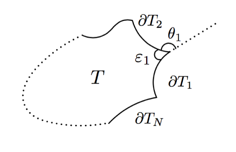
Figure 1: Gauss-Bonnet theorem. We consider a closed curve in a surface.

Here, we briefly mention the Gauss-Bonnet theorem. $T$ is a two-dimensional orientable surface. Differentiable curves $\partial T_{a}$ ($a=1,2,\cdots,N$) are its boundaries. Please see Figure 1 for the orientable surface. We denote the jump angles between the curves as $\theta_{a}$ ($a=1,2,\cdots,N$). The Gauss-Bonnet theorem: GB-theorem

$$\iint_{T}KdS+\sum_{a=1}^{N}\int_{\partial T_{a}}\kappa_{g}d\ell+\sum_{a=1}^{N}\theta_{a}=2\pi,$$ (8)

where $\ell$ means the line element of the boundary curve, $dS$ denotes the area element of the surface, $K$ means the Gaussian curvature of the surface $T$, $\kappa_{g}$ is the geodesic curvature of $\partial T_{a}$. The sign of $\ell$ is chosen to be consistent with the surface orientation.

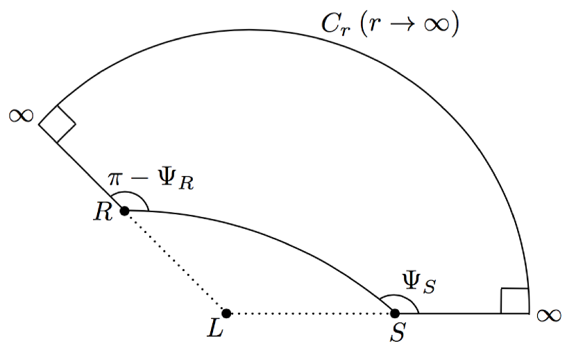
Figure 2: ${}^{\infty}_{R}{\square}^{\infty}_{S}$ is a quadrilateral embedded in a curved space.

Suppose a quadrilateral ${}^{\infty}_{R}{\square}^{\infty}_{S}$. Please see Figure 2 for this. This is made of four lines; (1) the spatial curve for the light ray, (2) and (3) two outgoing radial lines from R and from S and (4) a circular arc segment $C_{r}$ that is centered at the lens with the coordinate radius $r_{C}$ ($r_{C}\to\infty$) and intersects the radial lines at the receiver or the source. We restrict ourselves within the asymptotically flat spacetime. Then, $\kappa_{g}\to 1/r_{C}$ and $d\ell\to r_{C}d\phi$ as $r_{C}\to\infty$ (See e.g. GW2008 ). By using them, we find $\int_{C_{r}}\kappa_{g}d\ell\to\phi_{RS}$. Applying this result to the Gauss-Bonnet theorem for ${}^{\infty}_{R}{\square}^{\infty}_{S}$, we obtain

$$\alpha = \Psi_{R}-\Psi_{S}+\phi_{RS}$$ (9)

$$= -\iint_{{}^{\infty}_{R}{\square}^{\infty}_{S}}KdS.$$

Therefore, $\alpha$ is shown to be invariant for transformations of the spatial coordinates. In addition, $\alpha$ is well-defined even when $L$ is a singular point. This is because the point $L$ does not appear in the surface integral nor in the line integral. Furthermore, $\alpha$ vanishes in Euclidean space. This means $\alpha$ is a measure of the deviation from the flat space.

Figure 3: Observable $\alpha$ in Eq. (7). In this schematic figure, the lens, receiver and source are the Sun, the Earth and a pulsar that periodically radiates radio signals in a specific anistropic manner. From the pulse profile, we can determine the radiation direction at the source. By using the ephemeris, we know the relative positions of the Sun, Earth and the pulsar. Hence, we can determine $\phi_{RS}$ and $\Psi_{S}$. By observing the pulsar, we can measure $\Psi_{R}$. In principle, therefore, we can determine $\Psi_{R}-\Psi_{S}+\phi_{RS}$ from these astronomical observations.

Here, we explain that $\alpha$ defined in Eq. (7) is observable in principle. For the simplicity, let us imagine the following ideal situation. The positions of a source and receiver are known. For instance, we assume that the lens object is the Sun, the receiver is located at the Earth, and the source is a pulsar which radiates radio signals with a constant period in an anisotropic manner. In particular, we assume that the source is one of the known pulsars whose spin period and pulse signal behaviors such as pulse profiles are well-understood. By very accurate radio observations such as VLBI, the relative positions of the Earth, Sun and the pulsar can be determined from the ephemeris. (1) From this, we can know $\phi_{RS}$ in principle. (2) We can directly measure the angle $\Psi_{R}$ at the Earth between the solar direction and the pulsar direction. (3) More importantly, the direction of radiating the pulses that reaches the receiver can be also determined in principle, because the viewing angle of the pulsar seen by the receiver is known from the pulse profiles. The viewing angle is changing with time because of the Earth motion around the Sun. By using the pulsar position and the pulse radiation direction, we can determine $\Psi_{S}$. Please see Figure 3 for this situation. We explain in more detail how $\Psi_{S}$ at S can be measured by the observer at R. We consider a pulsar whose spin axis is known from some astronomical observations. A point is that the spin axis of an isolated pulsar is constant with time. The pulse shape and profile depend on the viewing angle with respect to the spin axis of the pulsar. The Earth moves around the Sun and hence the observer sees the same pulsar with different viewing angles with time. Accordingly, the observed pulse shape changes. By observing such a change in the pulse shape, we can in principle determine the intrinsic direction of the radio emission, namely the angle between the spin axis and the direction of the emitted light to the observer. In addition, we can know the intrinsic position (including the radial direction from the lens) of such a known pulsar from the ephemeris. By using the intrinsic position (its radial direction) and emission direction at S, $\Psi_{S}$ can be determined in principle, though it is very difficult with current technology. As a result, we can determine in principle $\Psi_{R}-\Psi_{S}+\phi_{RS}$ from astronomical observations. Namely, $\alpha$ in Eq. (7) is observable. Note that this procedure does not need assume a different spacetime, while such a fiducial spacetime was assumed by Arakida (2018) Arakida2018 , though the receiver in our universe cannot observe the fiducial different spacetime but can assume (or make theoretical calculations of) some quantities on the different spacetime.

One can easily see that, in the far limit of the source and the receiver, Eq. (9) agrees with the deflection angle of light as

$$\alpha_{\infty}=2\int_{0}^{u_{0}}\frac{du}{\sqrt{F(u)}}-\pi.$$ (10)

Here, we define $u$ and $u_{0}$ as as the inverse of $r$, the inverse of the closest approach (often denoted as $r_{0}$), respectively. $F(u)$ is defined as

$$F(u)\equiv\left(\frac{du}{d\phi}\right)^{2}.$$ (11)

$F(u)$ can be computed by using Eq. (3).

The present paper wishes to avoid the far limit in the following reason. Every observed stars and galaxies are never located at infinite distance from us. For instance, we observe finite-redshift galaxies in cosmology. We cannot see objects at infinite redshift (exactly at the horizon). Except for a few rare cases in astronomy, the distance to the light source is much larger than the size of the lens. Therefore, we find a strong motivation for studying a situation that the distance from the source to the receiver is finite. We define $u_{R}$ and $u_{S}$ as the inverse of $r_{R}$ and $r_{S}$, respectively, where $r_{R}$ and $r_{S}$ are finite. Eq. (7) is rewritten in an explicit form as Ishihara2016 ; Ishihara2017

$$\alpha=\int_{u_{R}}^{u_{0}}\frac{du}{\sqrt{F(u)}}+\int_{u_{S}}^{u_{0}}\frac{du}{\sqrt{F(u)}}+\Psi_{R}-\Psi_{S}.$$ (12)

Here, we assume light rays that have the only one local minimum of the radius coordinate between $r_{S}$ and $r_{R}$. This is valid for normal situations in astronomy. However, we should note that multiple local minima are possible, e.g. if the emitter or the receiver (or both) are between the horizon and the light sphere in the Schwarzschild spacetime, or if the emitter and receiver are at different sides of the throat of a wormhole spacetime. For such a case of multiple local minima, Eq. (12) has to be modified, because it assumes only the local minimum at $u=u_{0}$.

III Weak deflection of light in Schwarzschild spacetime

In this section, we consider the weak deflection of light in Schwarzschild spacetime, for which the line element becomes

$$ds^{2} = -\left(1-\frac{r_{g}}{r}\right)dt^{2}+\frac{dr^{2}}{\displaystyle 1-\frac{r_{g}}{r}}$$ (13)

$$+r^{2}(d\theta^{2}+\sin^{2}\theta d\phi^{2}),$$

where $r_{g}=2M$ in the geometrical unit. Then, $F(u)$ is

$$F(u)=\frac{1}{b^{2}}-u^{2}+r_{g}u^{3}.$$ (14)

By using Eq. (6), $\Psi_{R}-\Psi_{S}$ in the Schwarzschild spacetime is expanded as

$$\Psi_{R}^{\mbox{Sch}}-\Psi_{S}^{\mbox{Sch}} \equiv [\arcsin(bu_{R})+\arcsin(bu_{S})-\pi]$$ (15)

$$-\frac{1}{2}br_{g}\left(\frac{u_{R}^{2}}{\sqrt{1-b^{2}u_{R}^{2}}}+\frac{u_{S}^{2}}{\sqrt{1-b^{2}u_{S}^{2}}}\right)+O(br_{g}^{2}u_{S}^{3},br_{g}^{2}u_{R}^{3}).$$

Note that $\Psi_{R}-\Psi_{S}\to\pi$ in the Schwarzschild spacetime as $u_{S}\to 0$ and $u_{R}\to 0$.

IV Other examples

This section discusses two examples for a non-asymptotically flat spacetime. One is the Kottler solution to the Einstein equation. The other is an exact solution in the Weyl conformal gravity. The aim of this study is to give us a suggestion or a speculation. We note that the present formulation is limited within the asymptotic flatness, rigorously speaking. As mentioned in Introduction, Arakida Arakida2018 made an attempt to apply the Gauss-Bonnet theorem to quadrilaterals that are not extending to infinity, though a comparison between two different manifolds that he proposed is an open issue. A more careful study that gives a justification for this speculation or perhaps disprove it will be left for future.

In this section, we do not assume the source at the past null infinity ($r_{S}\to\infty$) nor the receiver at the future null infinity ($r_{R}\to\infty$), because $A(r)$ diverges or does not exist as $r\to\infty$. We keep in mind that the source and receiver are located at finite distance from the lens object. Therefore, we use Eq. (12). As mentioned already, Eq. (6) is more useful for calculating $\Psi_{R}$ and $\Psi_{S}$ than Eq. (5), because Eq. (6) requires only the local quantities but not any differentiation. By straightforward calculations, we obtain the following results for the above two models.

IV.1 Kottler solution

We consider the Kottler solution Kottler . This solution is written as

$$ds^{2} = -\left(1-\frac{2M}{r}-\frac{\Lambda}{3}r^{2}\right)dt^{2}+\frac{dr^{2}}{\displaystyle 1-\frac{2M}{r}-\frac{\Lambda}{3}r^{2}}$$ (16)

$$+r^{2}(d\theta^{2}+\sin^{2}\theta d\phi^{2}),$$

where the cosmological constant is denoted by $\Lambda$.

We use Eq. (6), such that $\Psi_{R}-\Psi_{S}$ can be expanded in terms of $2M$ and $\Lambda$ as

$$\Psi_{R}-\Psi_{S} =\Psi^{Sch}_{R}-\Psi^{Sch}_{S}-\frac{b\Lambda}{6u_{R}\sqrt{1-b^{2}u_{R}^{2}}}-\frac{b\Lambda}{6u_{S}\sqrt{1-b^{2}u_{S}^{2}}}$$

$$+\frac{bu_{R}(-1+2b^{2}u_{R}^{2})}{8(1-b^{2}u_{R}^{2})^{3/2}}\left(4M^{2}u_{R}^{2}+\frac{4M\Lambda}{3u_{R}}+\frac{\Lambda^{2}}{9u_{R}^{4}}\right)$$

$$+\frac{bu_{S}(-1+2b^{2}u_{S}^{2})}{8(1-b^{2}u_{S}^{2})^{3/2}}\left(4M^{2}u_{S}^{2}+\frac{4M\Lambda}{3u_{S}}+\frac{\Lambda^{2}}{9u_{S}^{4}}\right)$$

$$+O(M^{3},M^{2}\Lambda,M\Lambda^{2},\Lambda^{3}).$$ (17)

Here, $\Psi_{R}^{\mbox{Sch}}-\Psi_{S}^{\mbox{Sch}}$ is a pair of the terms that appear also in a case of the Schwarzschild spacetime. The above expansion of $\Psi_{R}-\Psi_{S}$ has a divergent term in the limit as $u_{S}\to 0$ and $u_{R}\to 0$. The reason for this divergent behavior is that the spacetime is not asymptotically flat and therefore the limit of $u_{S}\to 0$ and $u_{R}\to 0$ is no longer allowed. Hence, the power series in Eq. (17) is mathematically valid only within a convergence radius.

For the Kottler spacetime, $F(u)$ becomes

$$F(u)=\frac{1}{b^{2}}-u^{2}+r_{g}u^{3}+\frac{\Lambda}{3}.$$ (18)

We obtain

$$\phi_{RS}= \pi-\arcsin(bu_{R})-\arcsin(bu_{S})$$

$$+\frac{r_{g}}{b}\left[\frac{1}{\sqrt{1-b^{2}u_{R}^{2}}}\left(1-\frac{1}{2}b^{2}u_{R}^{2}\right)+\frac{1}{\sqrt{1-b^{2}u_{S}^{2}}}\left(1-\frac{1}{2}b^{2}u_{S}^{2}\right)\right]$$

$$+\frac{\Lambda b^{3}}{6}\left[\frac{u_{R}}{\sqrt{1-b^{2}u_{R}^{2}}}+\frac{u_{S}}{\sqrt{1-b^{2}u_{S}^{2}}}\right]+\frac{r_{g}\Lambda b}{12}\left[\frac{2-3b^{2}u_{R}^{2}}{(1-b^{2}u_{R}^{2})^{\frac{3}{2}}}+\frac{2-3b^{2}u_{S}^{2}}{(1-b^{2}u_{S}^{2})^{\frac{3}{2}}}\right]+O(r_{g}^{2},\Lambda^{2}).$$ (19)

By using Eqs. (17) and (19), $\alpha$ is obtained as

$$\alpha= \frac{r_{g}}{b}\left[\sqrt{1-b^{2}u_{R}^{2}}+\sqrt{1-b^{2}u_{S}^{2}}\right]$$

$$-\frac{\Lambda b}{6}\left[\frac{\sqrt{1-b^{2}u_{R}^{2}}}{u_{R}}+\frac{\sqrt{1-b^{2}u_{S}^{2}}}{u_{S}}\right]$$

$$+\frac{r_{g}\Lambda b}{12}\left[\frac{1}{\sqrt{1-b^{2}u_{R}^{2}}}+\frac{1}{\sqrt{1-b^{2}u_{S}^{2}}}\right]+O(r_{g}^{2},\Lambda^{2}).$$ (20)

This equation has several divergent terms as $bu_{R}\to 0$ and $bu_{S}\to 0$. The apparent divergent is problematic only in the case that the source or receiver is located at the horizon. In other words, all the terms in Eq. (20) are finite and thus harmless for astronomical situations.

IV.2 Weyl conformal gravity case

Next, we consider Weyl conformal gravity model. This theory was originally suggested by Bach Bach . The SSS solution in this model is expressed by introducing three new parameters that are often denoted as $\beta$, $\gamma$ and $k$. For this generalized solution in conformal gravity, Birkhoff’s theorem still holds Riegert . The SSS solution in the Weyl gravity model is MK

$$ds^{2} = -A(r)dt^{2}+\frac{1}{A(r)}dr^{2}+r^{2}(d\theta^{2}+\sin^{2}\theta d\phi^{2}),$$

$$A(r) = 1-3m\gamma-\frac{2m}{r}+\gamma r-kr^{2}.$$ (21)

Here, $m\equiv\beta(2-3\beta\gamma)/2$. $kr^{2}$ in the metric plays the same role as the cosmological constant in the Kottler spacetime that has been studied above. Therefore, we omit the $r^{2}$ term for simplifying our analysis.

By using Eq. (6), we expand $\Psi_{R}-\Psi_{S}$ in $\beta$ and $\gamma$. The result is

$$\Psi_{R}-\Psi_{S}\equiv \Psi_{R}^{\mbox{Sch}}-\Psi_{S}^{\mbox{Sch}}$$

$$+\frac{b\gamma}{2}\left(\frac{u_{R}}{\sqrt{1-b^{2}u^{2}_{R}}}+\frac{u_{S}}{\sqrt{1-b^{2}u^{2}_{S}}}\right)$$

$$-\frac{m\gamma}{2}\left[\frac{bu_{R}(2-b^{2}u_{R}^{2})}{(1-b^{2}u_{R}^{2})^{3/2}}+\frac{bu_{S}(2-b^{2}u_{S}^{2})}{(1-b^{2}u_{S}^{2})^{3/2}}\right]+O(m^{2},\gamma^{2}).$$ (22)

We should note that this expansion of $\Psi_{R}-\Psi_{S}$ is divergent as $u_{S}\to 0$ and $u_{R}\to 0$. This divergent behavior is not so problematic, because the limit of $u_{S}\to 0$ and $u_{R}\to 0$ is not allowed in this spacetime. Hence, we note that, rigorously speaking, Eq. (22) is mathematically valid only within a convergence radius.

For the present case omitting $k$, we obtain

$$F(u)=\frac{1}{b^{2}}-u^{2}+2mu^{3}+\gamma u^{2}-\gamma u.$$ (23)

$\phi_{RS}$ is computed as

$$\phi_{RS}= [\pi-\arcsin(bu_{R})-\arcsin(bu_{S})]$$

$$+\frac{m}{b}\left(\frac{2-b^{2}u_{R}^{2}}{\sqrt{1-b^{2}u_{R}^{2}}}+\frac{2-b^{2}u_{S}^{2}}{\sqrt{1-b^{2}u_{S}^{2}}}\right)$$

$$-\frac{\gamma}{2}\left(\frac{b}{\sqrt{1-b^{2}u_{R}^{2}}}+\frac{b}{\sqrt{1-b^{2}u_{R}^{2}}}\right)$$

$$+\frac{m\gamma}{2}\left[\frac{b^{3}u_{R}^{3}}{(1-b^{2}u_{R}^{2})^{3/2}}+\frac{b^{3}u_{S}^{3}}{(1-b^{2}u_{S}^{2})^{3/2}}\right]+O(m^{2},\gamma^{2}).$$ (24)

Consequently, we obtain $\alpha$ as

$$\alpha= \frac{2m}{b}\left(\sqrt{1-b^{2}u_{R}^{2}}+\sqrt{1-b^{2}u_{S}^{2}}\right)$$

$$-m\gamma\left(\frac{bu_{R}}{\sqrt{1-b^{2}u_{R}^{2}}}+\frac{bu_{S}}{\sqrt{1-b^{2}u_{S}^{2}}}\right)+O(m^{2},\gamma^{2}).$$ (25)

The linear terms in $\gamma$ cancel out with each other and they do not appear in the final expression for the deflection angle of light. This result may suggest a correction to the results in previous papers Edery ; Sultana ; Cattani that reported non-zero contributions from $\gamma$.

IV.3 Far source and receiver

Next, we investigate a situation of a distant source and receiver from the lens object: $bu_{S}\ll 1$ and $bu_{R}\ll 1$. Divergent terms in the deflection angle appear in the limit as $bu_{S}\to 0$. Therefore, We carefully investigate the leading part in a series expansion, where the infinite limit is not taken. As a result, approximate expressions for the deflection of light are obtained as follows.

(1) Kottler model:
The expression for $\phi_{RS}$ in this approximation is the same as the seventh and eighth terms of Eq. (5) in Sereno , the third and fifth terms of Eq. (15) in Bhadra , and the second term of Eq. (14) in ArakidaK . On the other hand, they Sereno ; Bhadra ; ArakidaK did not take account of $\Psi_{R}-\Psi_{S}$. In the far approximation, Eq. (20) becomes

$$\alpha\sim\frac{4M}{b}-\frac{1}{6}\Lambda b\left(\frac{1}{u_{R}}+\frac{1}{u_{S}}\right)+\frac{1}{3}M\Lambda b.$$ (26)

This expression suggestions a correction to the earlier works Sereno ; Bhadra ; ArakidaK . For instance, only the term of $\phi_{RS}$ was considered in Sereno (2009).

(2) Weyl conformal gravity model:
Next, we consider the Weyl conformal gravity model. The deflection angle of light in the far approximation is computed as

$$\alpha \sim \frac{4m}{b}+O(m^{2},\gamma^{2}),$$ (27)

where $m\gamma$ parts from $\Psi_{R}-\Psi_{S}$ and from $\psi_{RS}$ cancel out with each other. Please see also Eqs. (22) and (24). For instance, Reference Lim2017 gives the exact expression of the deflection angle for the asymptotic receiver and source in the Kottler and Weyl conformal gravity spacetime.

V Extension to the Strong deflection of light

In the previous sections, we considered the weak deflection of light: A light ray from the source to the receiver is expressed by a spatial curve. The curve is simply-connected. In the strong deflection limit, on the other hand, it is possible that the spatial curve has a winding number with intersection points. We thus divide the whole curve into segments. And it is easier to investigate each simple segment.

V.1 Loops in the photon orbit

We begin with one loop case of the light ray curve. This case is shown by Figure 4.

First, we consider the two quadrilaterals (1) and (2) in Figure 5. They can be constructed by introducing an auxiliary point (P) and next by adding auxiliary outgoing radial lines (solid line in this figure) from the point P in the quadrilaterals (1) and (2). The point P does not need to be the periastron. The direction of the two auxiliary lines in (1) and (2) is opposite to each other. The two auxiliary lines thus cancel out to make no contributions to $\alpha$. Here, $\theta_{1}$ and $\theta_{2}$ denote the inner angle at the point P in the quadrilateral (1) and that in the quadrilateral (2), respectively. We can see that $\theta_{1}+\theta_{2}=\pi$. This is because the line from the source to the receiver is a geodesic and the point P is located in this line.

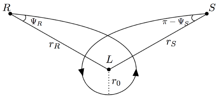
Figure 4: A one-loop case for the photon orbit in $M^{\mbox{opt}}$.

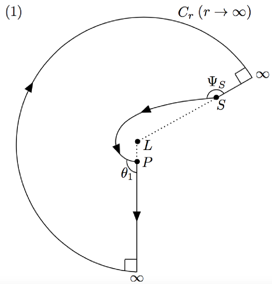
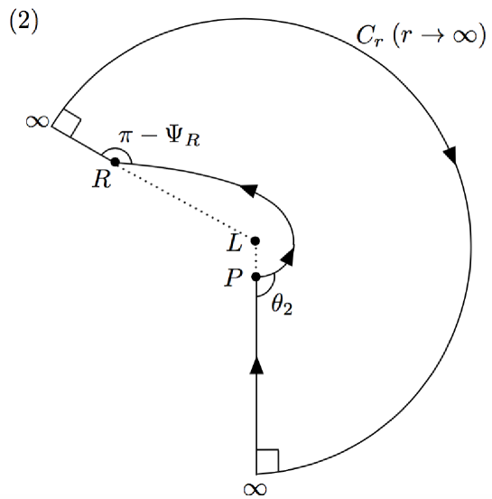
Figure 5: Quadrilaterals. They are made from the photon orbit in a non-Euclidean space. See Figure 4.

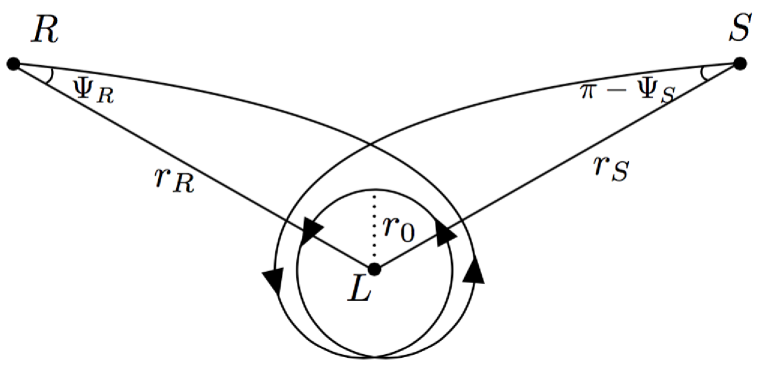
Figure 6: Two loops for the light ray in $M^{\mbox{opt}}$.

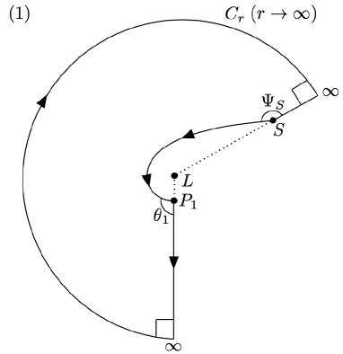
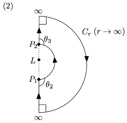
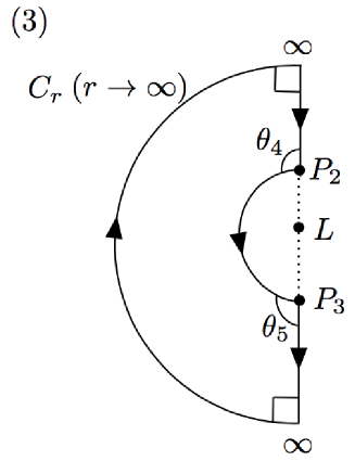
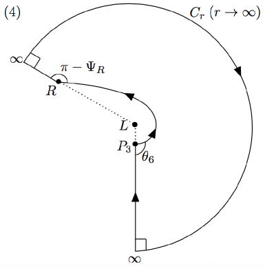
Figure 7: Quadrilaterals (1)-(4). They are in a non-Euclidean plane $M^{\mbox{opt}}$. See also Figure 6.

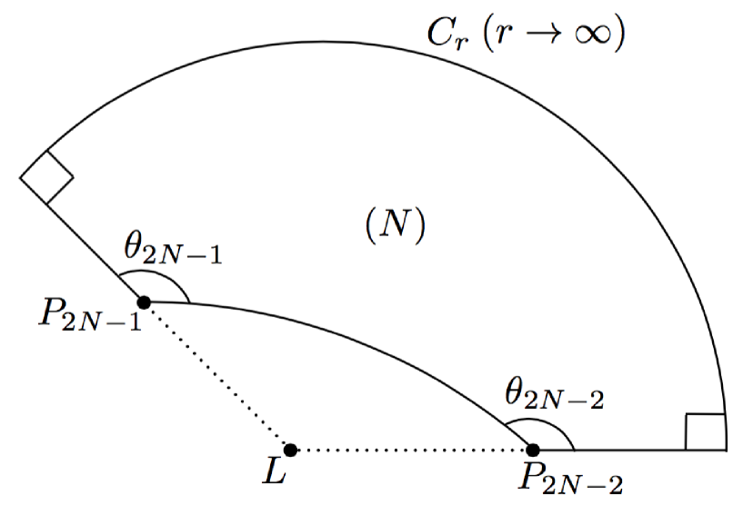
Figure 8: A quadrilateral in any loop number. This case is discussed when we prove by induction that Eq. (7) holds in any loop number.

For a quadrilateral in Figure 5, the method in Section II is still applicable. By the same way of obtaining Eq. (9), we obtain

$$\alpha^{(1)} =(\pi-\theta_{1})-\Psi_{S}+\phi_{RS}^{(1)},$$

$$\alpha^{(2)} =\Psi_{R}-\theta_{2}+\phi_{RS}^{(2)}.$$ (28)

Here, $\phi_{RS}$ is divided into two parts: One is $\phi_{RS}^{(1)}$ for one quadrilateral and the other is $\phi_{RS}^{(2)}$ for the other quadrilateral.

If $r_{S}=r_{R}$, the quadrilaterals (1) and (2) are symmetric for reflection and $\phi_{RS}^{(1)}=\phi_{RS}^{(2)}=\phi_{RS}/2$. If not, $\phi_{RS}^{(1)}$ is not the same as $\phi_{RS}^{(2)}$. In any case, however, $\phi_{RS}^{(1)}+\phi_{RS}^{(2)}=\phi_{RS}$. $\Psi_{S}$ and $(\pi-\Psi_{R})$ are the inner angles at $S$ and $R$, respectively. Therefore,

$$\alpha =\alpha^{(1)}+\alpha^{(2)}$$

$$=\Psi_{R}-\Psi_{S}+\phi_{RS},$$ (29)

where we use $\theta_{1}+\theta_{2}=\pi$ and $\phi_{RS}^{(1)}+\phi_{RS}^{(2)}=\phi_{RS}$. This result is the same as Eq. (7), though the validity domain is different.

Next, we investigate a case of two loops shown by Figure 6. For this case, we add lines in order to divide the shape into four quadrilaterals as shown by Figure 7. We immediately find

$$\alpha^{(1)} =(\pi-\theta_{1})-\Psi_{S}+\phi_{RS}^{(1)},$$

$$\alpha^{(2)} =(\pi-\theta_{3})-\theta_{2}+\phi_{RS}^{(2)},$$

$$\alpha^{(3)} =(\pi-\theta_{5})-\theta_{4}+\phi_{RS}^{(3)},$$

$$\alpha^{(4)} =\Psi_{R}-\theta_{6}+\phi_{RS}^{{(4)}},$$ (30)

where $\phi_{RS}^{(1)}+\phi_{RS}^{(2)}+\phi_{RS}^{(3)}+\phi_{RS}^{(4)}=\phi_{RS}$. Hence, we obtain

$$\alpha =\alpha^{(1)}+\alpha^{(2)}+\alpha^{(3)}+\alpha^{(4)}$$

$$=\Psi_{R}-\Psi_{S}+\phi_{RS},$$ (31)

where we use $\theta_{1}+\theta_{2}=\theta_{3}+\theta_{4}=\theta_{5}+\theta_{6}=\pi$. Eq. (31) is obtained for the two-loop case in the same form as Eq. (7). A loop does make the contribution to $\alpha$ only through the terms of $\phi_{RS}^{(2)}+\phi_{RS}^{(3)}$.

Finally, we shall complete the proof. We consider the arbitrary winding number, say $W$. For this case, we prepare $2W$ quadrilaterals. We denote the inner angles at finite distance from $L$ as $\theta_{0},\cdots,\theta_{2W}$ in order from $S$ to $R$ as shown by Figure 8. Here, $\theta_{0}=\Psi_{S}$ and $\theta_{2W}=\pi-\Psi_{R}$. Neighboring quadrilaterals (N) and (N+1) make the contribution to $\alpha$ only through $\phi_{RS}^{(N)}+\phi_{RS}^{(N+1)}$. We can understand this by noting that $\theta_{2N-1}+\theta_{2N}=\theta_{2N+1}+\theta_{2N+2}=\pi$ and the auxiliary lines cancel out. By induction, therefore, we complete the proof; Eq. (7) holds for any winding number.

Eq. (7) is equivalent to Eq. (12). This is shown by using the orbit equation. This expression is rearranged as

$$\alpha =\Psi_{R}-\Psi_{S}+\phi_{RS}$$

$$=\Psi_{R}-\Psi_{S}+\int^{0}_{u_{R}}\frac{du}{\sqrt{F(u)}}+\int^{0}_{u_{S}}\frac{du}{\sqrt{F(u)}}+2\int^{u_{0}}_{0}\frac{du}{\sqrt{F(u)}}.$$ (32)

We define the difference between the asymptotic deflection angle and the deflection angle for the finite distance case as $\delta\alpha$.

$$\delta\alpha\equiv\alpha-\alpha_{\infty}.$$ (33)

The meaning of this is the finite-distance correction to the deflection angle of light. By substituting Eqs. (10) and (32) into Eq. (33), we get

$$\delta\alpha=(\Psi_{R}-\Psi_{S}+\pi)+\int^{0}_{u_{R}}\frac{du}{\sqrt{F(u)}}+\int^{0}_{u_{S}}\frac{du}{\sqrt{F(u)}}.$$ (34)

This expression implies two origins of the finite-distance corrections. One origin is $\Psi_{R}$ and $\Psi_{S}$. They are angles that are defined in a curved space. The other origin is the two path integrals. They contain the information on the curved space. If we consider a receiver and source in the weak gravitational field (as common in astronomy), the finite-distance correction reflects only the weak field region, even if the light ray passes through a strong field region.

VI Strong deflection of light in Schwarzschild spacetime

In this section, we consider the Schwarzschild black hole. By using $F(u)$ given by Eq. (14), we solve Eq. (32) in an analytic manner. The exact expressions involve incomplete elliptic integrals of the first kind. When the distances from the lens to the source and the receiver are much larger than the impact parameter of light ($r_{S}\gg b,r_{R}\gg b$) but the light ray passes near the photon sphere ($r_{0}\sim 3M$), Eq. (32) becomes approximately

$$\alpha= \frac{2M}{b}\left[\sqrt{1-b^{2}u_{R}^{2}}+\sqrt{1-b^{2}u_{S}^{2}}-2\right]$$

$$+2\log\left(\frac{12(2-\sqrt{3})r_{0}}{r_{0}-3M}\right)-\pi$$

$$+O\left(\frac{M^{2}}{r_{R}{}^{2}},\frac{M^{2}}{r_{S}{}^{2}},1-\frac{3M}{r_{0}}\right),$$ (35)

where we used a logarithmic term Iyer in the last term of Eq. (32). Here, the dominant terms in $\Psi_{R}$ and $\Psi_{S}$ cancel with the terms in the integrals. As a consequence, $\Psi_{R}$ and $\Psi_{S}$ do not appear in the approximate expression of Eq. (35).

As mentioned above, it follows that the logarithmic term by the strong gravity is free from finite-distance corrections such as $\sqrt{1-(bu_{S})^{2}}$. By chance, $\delta\alpha$ in the strong deflection limit (See Eq. (32)) is apparently the same as that for the weak deflection case (See e.g. Eq. (29) in Ishihara2017 ). Therefore, the finite-distance correction in the strong deflection limit is again

$$\delta\alpha\sim O\left(\frac{Mb}{r_{S}{}^{2}}+\frac{Mb}{r_{R}{}^{2}}\right).$$ (36)

This is the same expression as that for the weak field case (e.g. Ishihara2016 ). Namely, the correction is linear in the impact parameter. The finite-distance correction in the weak deflection case (large $b$) is thus larger than that in the strong deflection one (small $b$), if the other parameters remain the same.

VI.1 Sagittarius A^∗

Next, we briefly mention an astronomical implication of the strong deflection. One of the most feasible candidates for the strong deflection is Sagittarius ^∗ (Sgr A^∗) that is located at our galactic center. In this case, the receiver distance is much larger than the impact parameter of light and a source star may live in the bulge of our Galaxy.

The apparent size of Sgr A^∗ is expected to be nearly the same as that of the central massive object of M87. However, the finite-distance correction to Sgr A^∗ becomes much larger than that to the M87 case, because Sgr A^∗ is much closer to us than M87.

For Sgr A^∗, Eq. (36) is evaluated as

$$\delta\alpha \sim\frac{Mb}{r_{S}{}^{2}}$$

$$\sim 10^{-5}\mbox{arcsec.}\times\left(\frac{M}{4\times 10^{6}M_{\odot}}\right)\left(\frac{b}{3M}\right)\left(\frac{0.1\mbox{pc}}{r_{S}}\right)^{2},$$ (37)

where the central black hole mass is assumed as $M\sim 4\times 10^{6}M_{\odot}$ and we take the limit of strong deflection $b\sim 3M$. Rather interestingly, this correction as $\sim 10^{-5}\mbox{arcsec.}$ will be reachable by the Event Horizon Telescope EHT and the near-future astronomy.

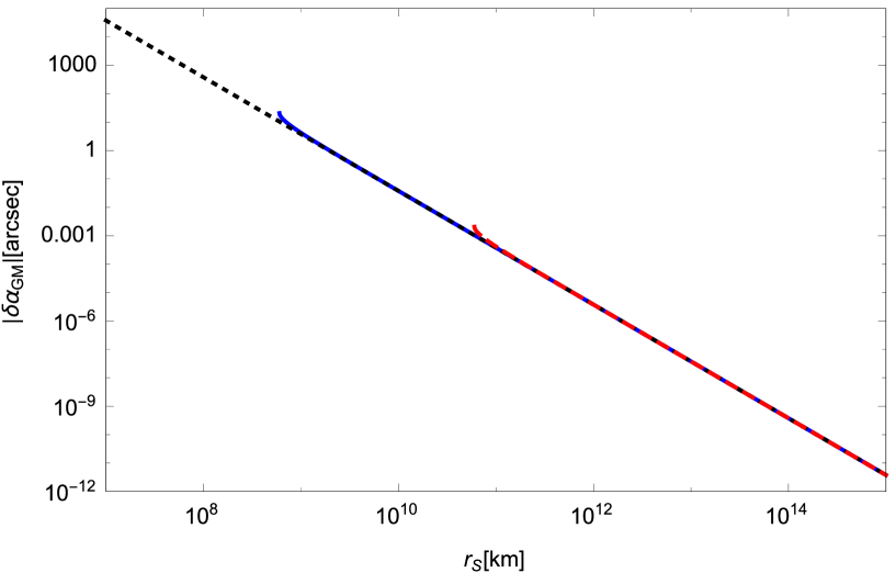
Figure 9: The finite-distance correction for the Sgr A^∗ as $\delta\alpha_{GM}$. The horizontal axis denotes the source distance $r_{S}$. The vertical one means the finite-distance correction to the light deflection. The solid line (blue in color) and dashed one (red in color) mean $b=10^{2}M$ and $b=10^{4}M$, respectively. The dotted curve (yellow in color) denotes the leading term of $\delta\alpha_{GM}$ given by Eq. (33). These three lines are substantially overlapped with each other. This implies that $\delta\alpha_{GM}$ is weakly dependent on the impact parameter $b$.

See Figure 9 for numerical estimations of the finite-distance correction by the source distance. This figure and Eq. (37) suggest that $\delta\alpha$ is $\sim$ ten (or more) micro arcseconds, if a source star is sufficiently close to Sgr A^∗, for instance within a tenth of one parsec from Sgr A^∗. For such a case, the infinite-distance limit does not hold, even though the source is still in the weak field. We should take account of finite-distance corrections that are discussed in this paper.

In the strong deflection case, each orbit around the black hole will have a slightly different $r_{0}$, thereby producing a number of ”ghost” images (often called relativistic images). In this paper, detailed calculations about it for the finite-distance source and receiver are not done. It is left for future.

VII Defining the gravitational deflection angle of light for a stationary and axially symmetric spacetime

VII.1 Optical metric for the stationary, axisymmetric spacetime

In this section, a stationary and axisymmetric spacetime is considered, for which we shall discuss how to define the gravitational deflection angle of light especially with using the Gauss-Bonnet theorem Ono2017 . The line element in this spacetime is Lewis ; LR ; Papapetrou

$$ds^{2}= g_{\mu\nu}dx^{\mu}dx^{\nu}$$

$$= -A(y^{1},y^{2})dt^{2}-2H(y^{1},y^{2})dtd\phi$$

$$+F(y^{1},y^{2})\gamma_{pq}dy^{p}dy^{q}+D(y^{1},y^{2})d\phi^{2}.$$ (38)

Here, $p,q$ mean $1$ and $2$, $\gamma_{pq}$ is a two-dimensional symmetric tensor, $\mu,\nu$ take from $0$ to $3$, $t$ and $\phi$ coordinates respect the Killing vectors. We rewrite this metric into a form, such that $\gamma_{pq}$ can be diagonal. We prefer to use the polar coordinates rather than the cylindrical ones, because the Kerr metric and the rotating Teo wormhole one are usually expressed in the polar coordinates. In the polar coordinates, Eq. (38) is rewritten as Metric

$$ds^{2}= -A(r,\theta)dt^{2}-2H(r,\theta)dtd\phi$$

$$+B(r,\theta)dr^{2}+C(r,\theta)d\theta^{2}+D(r,\theta)d\phi^{2},$$ (39)

where a local reflection symmetry is assumed with respect to the equatorial plane $\theta=\frac{\pi}{2}$. This assumption is expressed as

$$\left.\frac{\partial g_{\mu\nu}}{\partial\theta}\right|_{\theta=\frac{\pi}{2}}=0.$$ (40)

The functions are $A(r,\theta)>0,B(r,\theta)>0,C(r,\theta)>0,D(r,\theta)>0$ and $H(r,\theta)>0$. This assumption by Eq. (40) is needed for the existence of a photon orbit on the equatorial plane. Note that we do not assume the global reflection symmetry with respect to the equatorial plane.

The null condition $ds^{2}=0$ is solved for $dt$ as Civita ; AK

$$dt= \sqrt{\gamma_{ij}dx^{i}dx^{j}}+\beta_{i}dx^{i},$$ (41)

where $i,j$ denote from $1$ to $3$, $\gamma_{ij}$ and $\beta_{i}$ are defined as

$$\gamma_{ij}dx^{i}dx^{j}\equiv \frac{B(r,\theta)}{A(r,\theta)}dr^{2}+\frac{C(r,\theta)}{A(r,\theta)}d\theta^{2}+\frac{A(r,\theta)D(r,\theta)+H^{2}(r,\theta)}{A^{2}(r,\theta)}d\phi^{2},$$ (42)

$$\beta_{i}dx^{i}\equiv -\frac{H(r,\theta)}{A(r,\theta)}d\phi.$$ (43)

This spatial metric $\gamma_{ij}(\neq g_{ij})$ is used in order to define the arc length ($\ell$) along the photon orbit as

$$d\ell^{2}\equiv\gamma_{ij}dx^{i}dx^{j},$$ (44)

for which we define $\gamma^{ij}$ by $\gamma^{ij}\gamma_{jk}=\delta^{i}_{~{}k}$. $\gamma_{ij}$ defines a 3-dimensional Riemannian space ${}^{(3)}M$, where the photon orbit is a spatial curve. In the Appendix of Ref. AK , they show that $\ell$ is an affine parameter of a light ray.

If the spacetime is static, spherically symmetric and asymptotically flat, $\beta_{i}$ is zero and $\gamma_{ij}$ is nothing but the optical metric. The photon orbit follows a geodesic in a 3-dimensional Riemannian space. In this section and after, we refer to $\gamma_{ij}$ as the generalized optical metric. Note that the metric $\gamma_{ij}$ has been called the Fermat metric and the one-form $\beta_{i}$ the Fermat one-form by some authors.

We apply Gauss-bonnet theorem to a surface (See Figure 1). The Gauss-Bonnet theorem is expressed as

$$\iint_{{}^{R_{\infty}}_{R}{}^{S_{\infty}}_{S}}KdS+\int^{S}_{R}\kappa_{g}d\ell+\int^{R_{\infty}}_{S_{\infty}}\bar{\kappa}_{g}d\ell+[\Psi_{R}+(\pi-\Psi_{S})+\pi]=2\pi,$$ (45)

where we note that the geodesic curvatures of the path from $S$ to $S_{\infty}$ and the path from $R$ to $R_{\infty}$ are both $0$, because these paths are geodesic. $\kappa_{g}$ is the geodesic curvature of the photon orbit and $\bar{\kappa}_{g}$ is the geodesic curvature of the circular arc segment with an infinite radius.

VII.2 Gaussian curvature

In this subsection, we examine whether or not the rotational part ($\beta_{i}$) of the spacetime makes a contribution to the Gaussian curvature. The Gaussian curvature on the equatorial plane is expressed by using the 2-dimensional Riemann tensor ${}^{(2)}R_{r\phi r\phi}$ as

$$K= \frac{{}^{(2)}R_{r\phi r\phi}}{\det{\gamma^{(2)}_{ij}}}$$

$$= \frac{1}{\sqrt{\det{\gamma^{(2)}_{ij}}}}\left[\frac{\partial}{\partial\phi}\left(\frac{\sqrt{\det{\gamma^{(2)}_{ij}}}}{\gamma^{(2)}_{rr}}{{}^{(2)}\Gamma^{\phi}}_{rr}\right)-\frac{\partial}{\partial r}\left(\frac{\sqrt{\det{\gamma^{(2)}_{ij}}}}{\gamma^{(2)}_{rr}}{{}^{(2)}\Gamma^{\phi}}_{r\phi}\right)\right],$$ (46)

where ${}^{(2)}R_{r\phi r\phi}$ and ${}^{(2)}{\Gamma^{\i}}_{jk}$ are defined by using the generalized optical metric $\gamma_{ij}$ on the equatorial plane. $\det{\gamma^{(2)}_{ij}}$ is the determinant of the generalized optical metric in the equatorial plane.

$dS$ in Eq.(45) becomes

$$dS=\sqrt{\det\gamma^{(2)}}drd\phi.$$ (47)

The surface integration of the Gaussian curvature in Eq.(45) is rewritten explicitly as

$$\iint_{{}^{R_{\infty}}_{R}\square^{S_{\infty}}_{S}}KdS=\int^{\phi_{R}}_{\phi_{S}}\int^{\infty}_{r_{OE}}K\sqrt{\det\gamma^{(2)}}drd\phi,$$ (48)

where $r_{OE}$ means the solution of the orbit equation.

VII.3 Geodesic curvature

Let us imagine a parameterized curve in a surface. Roughly speaking, the geodesic curvature of the parameterized curve is a measure of how different the curve is from the geodesic. The geodesic curvature of the parameterized curve is defined as the surface-tangential component of the acceleration (namely the geodesic curvature) of the curve. The normal curvature is defined as the surface-normal component of the acceleration. The normal curvature does not appear in the present paper, because we consider only the curves on the equatorial plane.

The geodesic curvature in the vector form is defined as (see e.g. Math )

$$\kappa_{g}\equiv\bm{T}^{\prime}\cdot\left(\bm{T}\times\bm{N}\right),$$ (49)

where, for a parameterized curve, $\bm{T}$ denotes the unit tangent vector for the curve by reparameterizing the curve using its arc length, $\bm{T}^{\prime}$ means its derivative with respect to the parameter, and $\bm{N}$ indicates the unit normal vector for the surface. The geodesic curvature of a curve vanishes, if the curve follows the geodesic. This zero is because the acceleration vector $\bm{T}^{\prime}$ vanishes.

VII.4 Photon orbit with the generalized optical metric

In this subsection, we discuss geometrical aspects of a photon orbit in terms of the generalized optical metric. The unit vector tangent to the spatial curve is generally expressed as

$$e^{i}\equiv\frac{dx^{i}}{d\ell},$$ (50)

where a parameter $\ell$ is defined by Eq.(44).

The flight time $T$ of a light from the source to the receiver is obtained by performing the integral of Eq.(41),

$$T=\int^{t_{R}}_{t_{S}}dt=\int^{R}_{S}\left(\sqrt{\gamma_{ij}de^{i}de^{j}}+\beta_{i}de^{i}\right)d\ell.$$ (51)

The light ray follows the Fermat’s principle, namely $\delta T=0$ PerlickBook . The Lagrangian for a photon can be expressed as

$$\mathcal{L}=\sqrt{\gamma_{ij}e^{i}e^{j}}+\beta_{i}e^{i}.$$ (52)

From this, We obtain

$$\frac{d}{d\ell}\frac{\partial\mathcal{L}}{\partial e^{k}}= \gamma_{ik}{e^{i}}_{,l}e^{l}+\gamma_{ik,l}e^{i}e^{l}+\beta_{k,i}e^{i},$$ (53)

$$\frac{\partial\mathcal{L}}{\partial x^{k}}= \frac{1}{2}\gamma_{ij,k}e^{i}e^{j}+\beta_{i,k}e^{i},$$ (54)

where we used $\gamma_{ij}e^{i}e^{j}=1$ and the comma (,) defines the partial derivative. The Euler-Lagrange equation is calculated as

$${e^{j}}_{,l}e^{l}+\gamma^{kj}\left(\gamma_{ik,l}e^{i}e^{l}-\frac{1}{2}\gamma_{il,k}e^{i}e^{l}\right)=\gamma^{kj}(\beta_{l,k}-\beta_{k,l})e^{l}.$$ (55)

This leads to the equation for the light ray as AK

$$\frac{de^{i}}{d\ell}=-\gamma^{il}(\gamma_{lj,k}-\frac{1}{2}\gamma_{jk,l})e^{j}e^{k}+\gamma^{ij}(\beta_{k,j}-\beta_{j,k})e^{k}.$$

Therefore, the geodesic equation is equivalent to

$${e^{i}}_{|j}e^{j}= \frac{de^{i}}{d\ell}+{}^{(3)}{\Gamma^{i}}_{jk}e^{j}e^{k}$$

$$= \frac{de^{i}}{d\ell}+\gamma^{il}(\gamma_{lj,k}-\frac{1}{2}\gamma_{jk,l})e^{j}e^{k}$$

$$= \gamma^{ij}(\beta_{k,j}-\beta_{j,k})e^{k},$$ (56)

where we define $|$ as the covariant derivative with respect to $\gamma_{ij}$ . ${}^{(3)}\Gamma^{i}_{~{}jk}$ means the Christoffel symbol by $\gamma_{ij}$.

The acceleration vector $a^{i}$ is defined by

$$a^{i}\equiv{e^{i}}_{|j}e^{j}=\gamma^{ij}(\beta_{k|j}-\beta_{j|k})e^{k}=\gamma^{ij}(\beta_{k,j}-\beta_{j,k})e^{k}.$$ (57)

By using the Levi-Civita symbol $\varepsilon_{ijk}$, we express the cross (outer) product of $\bm{A}$ and $\bm{B}$ in the covariant manner

$$\sqrt{\gamma}\varepsilon_{ijk}A^{j}B^{k}=(\bm{A}\times\bm{B})_{i}.$$ (58)

The Levi-Civita tensor $\epsilon_{ijk}$ is defined by $\epsilon_{ijk}\equiv\sqrt{\gamma}\varepsilon_{ijk}$, where and $\varepsilon_{ijk}$ is the Levi-Civita symbol ($\varepsilon_{123}=1$). The Levi-Civita tensor $\epsilon_{ijk}$ in a three-dimensional satisfies

$$\epsilon_{sjk}\epsilon^{slm}=\sqrt{\gamma}\varepsilon_{sjk}\frac{1}{\sqrt{\gamma}}\varepsilon^{slm}=\delta_{j}^{l}\delta_{k}^{m}-\delta_{j}^{m}\delta_{k}^{l},$$ (59)

$$\epsilon_{sjk}\epsilon^{s}_{~{}lm}=\gamma_{jl}\gamma_{km}-\gamma_{jm}\gamma_{kl}.$$ (60)

By using Eqs.(58), (59) and (60), Eq.(57) is rewritten as

$$a^{i}=\gamma^{ij}e^{k}\epsilon_{sjk}(\nabla\times\bm{\beta})^{s}.$$ (61)

The vector $a^{i}$ is the spatial vector representing the acceleration due to $\beta_{i}$. In particular, $a^{i}$ is caused in gravitomagnetism Kopeikin . To be more precise, the gravitomagnetic vector has an analogy to the Lorentz force in electromagnetism $\propto\bm{v}\times(\bm{\nabla}\times\bm{A}_{m}$), in which $\bm{A}_{m}$ denotes the vector potential. The vector potential is defined as $\bm{B}=\nabla\times\bm{A}_{m},\bm{E}=-\nabla\phi-\frac{\partial\bm{A}_{m}}{\partial t},$ where $\bm{E}$ and $\bm{B}$ are the electric and magnetic fields, respectively, and the electric potential is $\phi$.

$\gamma_{ij}$ is not an induced metric but the generalized optical metric. If $\beta_{i}$ is non-vanishing, the photon orbit may be different from a geodesic in ${}^{(3)}M$ with $\gamma_{ij}$, even though the light ray in the four-dimensional spacetime follows the null geodesic.

In a stationary and axisymmetric spacetime, it is always possible to find out coordinates, such that $g_{0i}$ can vanish and $a^{i}=0$. In this case, the photon orbit is considered a spatial geodesic curve in ${}^{(3)}M$.

We study axisymmetric cases, which allow $g_{0i}\neq 0$. Therefore, geodesic curvature $\kappa_{g}$ does not always vanish in the photon orbit in the Gauss-Bonnet theorem, because the geodesic curvature $\kappa_{g}$ for a photon orbit is owing to the gravitomagnetic effect. This non-vanishing $\kappa_{g}$ for the photon orbit leads to a crucial difference from the SSS case Ishihara2016 ; Ishihara2017 .

VII.5 Geodesic curvature of a photon orbit

Eq. (49) is rearranged to be in the tensor form as

$$\kappa_{g}=\epsilon_{ijk}N^{i}a^{j}e^{k},$$ (62)

where $\vec{T}$ and $\vec{T}^{\prime}$ are corresponding to $e^{k}$ and $a^{j}$, respectively.

In this paper, the acceleration vector of the photon orbit depends on $\beta_{i}$. Hence, the geodesic curvature for the photon orbit also depends on it. A non-vanishing integral of the geodesic curvature along the light ray appears in the Gauss-Bonnet theorem Eq. (8).

Substituting Eq. (57) into $a^{i}$ in Eq. (62) leads to

$$\kappa_{g}= \epsilon_{ijk}N^{i}\gamma^{jl}(\beta_{n|l}-\beta_{l|n})e^{n}e^{k}$$

$$= \gamma^{ja}N^{i}e^{k}e^{b}\epsilon_{ijk}\epsilon_{sab}\epsilon^{sml}\beta_{l|m}$$

$$= N_{i}e_{k}e^{b}({\delta^{i}}_{s}{\delta^{k}}_{b}-{\delta^{i}}_{b}{\delta^{k}}_{s})\epsilon^{sml}\beta_{l|m}$$

$$= -\epsilon^{ijk}N_{i}\beta_{j|k},$$ (63)

where we used $\gamma_{ij}e^{i}e^{j}=1$ and $\gamma_{ij}e^{i}N^{j}=0$. The unit vector normal to the equatorial plane is

$$N_{p}=\frac{1}{\sqrt{\gamma^{\theta\theta}}}\delta_{p}^{\theta},$$ (64)

where the upward direction is chosen without loss of generality.

For the equatorial plane, we obtain

$$\epsilon^{\theta pq}\beta_{q|p} =-\frac{1}{\sqrt{\gamma}}\beta_{\phi,r},$$ (65)

where we use $\epsilon^{\theta r\phi}=-1/\sqrt{\gamma}$ and $\beta_{r,\phi}=0$ because of the axisymmetry.

By using Eqs. (64) and (65), $\kappa_{g}$ in Eq. (63) becomes

$$\kappa_{g}=-\frac{1}{\sqrt{\gamma\gamma^{\theta\theta}}}\beta_{\phi,r}.$$ (66)

By using Eq.(44), the line element in the path integral is obtained as

$$d\ell=\sqrt{\gamma_{rr}\left(\frac{dr}{d\phi}\right)^{2}+\gamma_{\phi\phi}}d\phi,$$ (67)

where $\theta=\pi/2$.

VII.6 Geodesic curvature of a circular arc segment

In a flat space, the geodesic curvature $\kappa$ of the circular arc segment of radius $R$ is obtained as

$$\kappa=\frac{1}{R}.$$ (68)

The geodesic curvature $\bar{\kappa}_{g}$ of a circular arc segment of radius $R_{c}=R_{\infty}$ is obtained as

$$\bar{\kappa}_{g}=\frac{1}{R}_{c},$$ (69)

where the radius $R_{c}$ is sufficiently larger than $r_{R}$ and $r_{S}$, and the circular arc segment is in the asymptotically flat region.

Eq.(44) becomes $d\ell^{2}=dr^{2}+r^{2}(d\theta^{2}+\sin^{2}\theta d\phi^{2})$, because we assume an asymptotically flat spacetime. Hence, the line element in the path integral of $\bar{\kappa}_{g}$ is obtained as

$$d\ell=R_{c}d\phi,$$ (70)

where we choose $\theta=\pi/2$ and $r=R_{c}$ for the circular arc segment.

Therefore, the path integral of $\bar{\kappa}_{g}$ in Eq.(45) is rewritten as

$$\int^{R_{\infty}}_{S_{\infty}}\bar{\kappa}_{g}d\ell=\int^{\phi_{R}}_{\phi_{S}}d\phi=\phi_{R}-\phi_{S}=\phi_{RS},$$ (71)

where we denote the angular coordinate values of the receiver and the source as $\phi_{R}$ and $\phi_{S}$, respectively.

VII.7 Impact parameter and light rays

By using Eq. (39), we study the orbit equation on the equatorial plane. The Lagrangian for a photon in the equatorial plane is obtained as

$$\hat{\mathcal{L}}=-A(r)\dot{t}^{2}-2H(r)\dot{t}\dot{\phi}+B(r)\dot{r}^{2}+D(r)\dot{\phi}^{2},$$ (72)

where the dot denotes the derivative with respect to the affine parameter and the functions $A(r),B(r),D(r),H(r)$ mean, to be rigorous, $A(r,\pi/2),B(r,\pi/2),D(r,\pi/2),H(r,\pi/2)$ respectively.

The metric (or the Lagrangian $\hat{\mathcal{L}}$ in the 4-dimensional spacetime) is independent of $t$ and $\phi$. Therefore,

$$\frac{d}{d\ell}\frac{\partial\hat{\mathcal{L}}}{\partial\dot{t}}=0,$$

$$\frac{d}{d\ell}\frac{\partial\hat{\mathcal{L}}}{\partial\dot{\phi}}=0.$$

Then, associated with the two Killing vectors $\xi^{\mu}=(1,0,0,0)$ and $\bar{\xi}^{\mu}=(0,0,0,1)$, respectively,

$$\frac{\partial\hat{\mathcal{L}}}{\partial\dot{t}}=g_{\mu\nu}\xi^{\mu}k^{\nu},$$

$$\frac{\partial\hat{\mathcal{L}}}{\partial\dot{\phi}}=g_{\mu\nu}\bar{\xi}^{\mu}k^{\nu},$$ (73)

where $k^{\mu}=\frac{dx^{\mu}}{d\ell}$ is the vector tangent to the light ray in the four-dimensional spacetime. There are two constants of motion

$$E =A(r)\dot{t}+H(r)\dot{\phi},$$ (74)

$$L =D(r)\dot{\phi}-H(r)\dot{t},$$ (75)

where $E$ denotes the energy of the photon and $L$ means the angular momentum of the photon. The impact parameter of the photon is defined as

$$b \equiv\frac{L}{E}$$

$$=\frac{-H(r)\dot{t}+D(r)\dot{\phi}}{A(r)\dot{t}+H(r)\dot{\phi}}$$

$$=\cfrac{-H(r)+D(r)\cfrac{d\phi}{dt}}{A(r)+H(r)\cfrac{d\phi}{dt}}.$$ (76)

In terms of the impact parameter $b$, $\hat{\mathcal{L}}=0$ can be considered as the orbit equation

$$\left(\frac{dr}{d\phi}\right)^{2}=\frac{A(r)D(r)+H^{2}(r)}{B(r)}\frac{D(r)-2H(r)b-A(r)b^{2}}{\left[H(r)+A(r)b\right]^{2}},$$ (77)

where we used Eq.(39). By introducing $u\equiv 1/r$, we rewrite the orbit equation as

$$\left(\frac{du}{d\phi}\right)^{2}=F(u),$$ (78)

where $F(u)$ is

$$F(u)=\frac{u^{4}(AD+H^{2})(D-2Hb-Ab^{2})}{B(H+Ab)^{2}}.$$ (79)

We examine the angles ($\Psi_{R},\Psi_{S}$ in figure 10) at the receiver position and the source one. The unit vector tangent to the photon orbit in ${}^{(3)}M$ is $e^{i}$. Its components on the equatorial plane are expressed as

$$e^{i}=\frac{1}{\xi}\Big{(}\frac{dr}{d\phi},0,1\Big{)},$$ (80)

where $\xi$ satisfies

$$\frac{1}{\xi}=\frac{A(r)[H(r)+A(r)b]}{A(r)D(r)+H^{2}(r)}.$$ (81)

This can be derived also from $\gamma_{ij}e^{i}e^{j}=1$ by using Eq. (77).

In the equatorial plane, the unit radial vector is

$$R^{i}=\Big{(}\frac{1}{\sqrt{\gamma_{rr}}},0,0\Big{)},$$ (82)

where the outgoing direction is chosen for a sign convention.

By using the inner product between $e^{i}$ and $R^{i}$, therefore, we define the angle as

$$\cos\Psi\equiv \gamma_{ij}e^{i}R^{j}$$

$$= \sqrt{\gamma_{rr}}\frac{A(r)[H(r)+A(r)b]}{A(r)D(r)+H^{2}(r)}\frac{dr}{d\phi},$$ (83)

where Eqs. (80), (81) and (82) are used. This is rewritten as

$$\sin\Psi= \frac{H(r)+A(r)b}{\sqrt{A(r)D(r)+H^{2}(r)}},$$ (84)

where Eq. (77) is used. We should note that $\sin\Psi$ in Eq. (84) is more useful in practical calculations, because it needs only the local quantities. On the other hand, $\cos\Psi$ by Eq. (83) needs the derivative as $dr/d\phi$. In addition, the domain of this $\Psi$ is $0\leq\Psi\leq\pi$ and hence $\sin\Psi$ is always positive.

By substituting $r_{R}$ and $r_{S}$ into $r$ of Eq.(84), we obtain $\sin\Psi_{R}$ and $\sin\Psi_{S}$, respectively. We note that the range of the principal value of $y=\arcsin x$ is $-\frac{\pi}{2}\leq y\leq\frac{\pi}{2}$ as usual. However, the range of $\Psi_{R}$ ($\Psi_{S}$) is $0\leq\Psi_{R}$($\Psi_{S}$)$\leq\pi$. By using the usual principal value, Eq.(84) for ($\Psi_{R}$) and ($\Psi_{S}$) become

$$\sin\Psi_{R}= \frac{H(r_{R})+A(r_{R})b}{\sqrt{A(r_{R})D(r_{R})+H^{2}(r_{R})}},$$ (85)

$$\sin(\pi-\Psi_{S})= \frac{H(r_{S})+A(r_{S})b}{\sqrt{A(r_{S})D(r_{S})+H^{2}(r_{S})}},$$ (86)

respectively, because $\Psi_{R}$ is an acute angle and $\Psi_{S}$ is an obtuse angle as shown by figure 10.

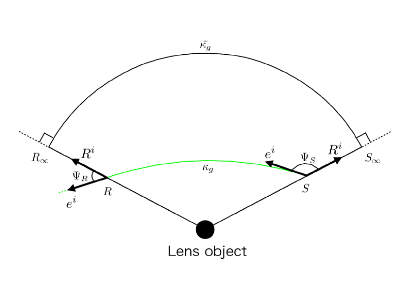
Figure 10: $\Psi_{R}$ and $\Psi_{S}$. $\Psi_{R}$ is the angle between the radial direction and the light ray at the receiver position. $\Psi_{S}$ is that at the source position.

VII.8 Gravitational deflection light in the axisymmetric case

We define

$$\alpha\equiv\Psi_{R}-\Psi_{S}+\phi_{RS},$$ (87)

for the equatorial plane in the axisymmetric spacetime. This definition apparently depends on the angular coordinate $\phi$. By using the Gauss-Bonnet theorem Eq. (8), this equation is rearranged as

$$\alpha=-\iint_{{}^{\infty}_{R}\square^{\infty}_{S}}KdS-\int_{R}^{S}\kappa_{g}d\ell.$$ (88)

Here, $d\ell$ is positive when the photon is in the prograde motion, whereas it is negative for the retrograde case. Eq. (88) means that $\alpha$ is coordinate-invariant for the axisymmetric case. Up to now, we do not use any equation for gravitational fields. Therefore, the above discussion and results still stand not only in the theory of general relativity but also in a general class of metric theories of gravity, only if the light ray in the four-dimensional spacetime is a null geodesic.

VIII Weak deflection of light in Kerr spacetime

VIII.1 Kerr spacetime and $\gamma_{ij}$

In this section, we focus on the weak deflection of light in the Kerr spacetime as an axisymmetric example. Kerr metric in the Boyer-Lindquist form is expressed as

$$ds^{2}= -\left(1-\frac{2Mr}{\Sigma}\right)dt^{2}-\frac{4aMr\sin^{2}\theta}{\Sigma}dtd\phi$$

$$+\frac{\Sigma}{\Delta}dr^{2}+\Sigma d\theta^{2}+\left(r^{2}+a^{2}+\frac{2a^{2}Mr\sin^{2}\theta}{\Sigma}\right)\sin^{2}\theta d\phi^{2},$$ (89)

where $\Sigma$ and $\Delta$ are defined as

$$\Sigma \equiv r^{2}+a^{2}\cos^{2}\theta,$$ (90)

$$\Delta \equiv r^{2}-2Mr+a^{2}.$$ (91)

Using the Gauss Bonnet theorem, the deflection angle of light in the Kerr spacetime was calculated for the asymptotic source and receiver by Werner Werner2012 . However, his method based on the osculating metric is limited within the asymptotic case. Later, Ono et al. developed a different approach using the Gauss-Bonnet theorem that enables to calculate the deflection angle for the finite distance case in the Kerr spacetime Ono2017 .

By using Eqs. (42) and (43), the generalized optical metric $\gamma_{ij}$ and the gravitomagnetic term $\beta_{i}$ for the Kerr metric are obtained as

$$\gamma_{ij}dx^{i}dx^{j}= \frac{\Sigma^{2}}{\Delta(\Sigma-2Mr)}dr^{2}+\frac{\Sigma^{2}}{(\Sigma-2Mr)}d\theta^{2}$$

$$+\left(r^{2}+a^{2}+\frac{2a^{2}Mr\sin^{2}\theta}{(\Sigma-2Mr)}\right)\frac{\Sigma\sin^{2}\theta}{(\Sigma-2Mr)}d\phi^{2},$$ (92)

$$\beta_{i}dx^{i}= -\frac{2aMr\sin^{2}\theta}{(\Sigma-2Mr)}d\phi.$$ (93)

Note that $\gamma_{ij}$ has no linear terms in the Kerr spin parameter $a$, because only $g_{0i}$ in $g_{\mu\nu}$ has a linear term in $a$ and $g_{0i}\propto H$ contributes to $\gamma_{ij}$ through a quadratic term $g_{0i}g_{0j}\propto H^{2}$ as shown by Eq. (42).

In order to calculate the Gaussian curvature $K$ of the equatorial plane, the geodesic curvature $\kappa_{g}$ of the light ray and the geodesic curvature $\bar{\kappa_{g}}$ of the circular arc of an infinite radius and the angles $\Psi_{R}$ and $\Psi_{S}$, we use two approximations for the weak field and slow rotation, where $M$ and $a$ play a role of book-keeping parameters though they are dimensional quantities.

By using Eq.(77), we obtain the orbit equation

$$\left(\frac{dr}{d\phi}\right)^{2}= \frac{b^{2}\left\{\frac{a^{2}}{b^{2}}+\frac{r}{b}(\frac{r}{b}-\frac{2M}{b})\right\}^{2}\left\{\frac{a^{2}}{b^{2}}(\frac{2M}{b}+\frac{r}{b})-\frac{4aM}{b^{2}}+\frac{2M}{b}-\frac{r}{b}+\frac{r^{3}}{b^{3}}\right\}}{\frac{r}{b}\{\frac{2aM}{b^{2}}+\frac{r}{b}-\frac{2M}{b}\}^{2}}$$

$$= \frac{r^{4}}{b^{2}}-r^{2}+2Mr-\frac{4r^{3}}{b^{3}}aM+\mathcal{O}(a^{2}),$$ (94)

where the weak-field and slow-rotation approximations are used in the last line. There are no $M$-squared terms in the last line. The orbit equation becomes

$$\left(\frac{du}{d\phi}\right)^{2}=F(u)=\frac{1}{b^{2}}-u^{2}+2Mu^{3}-\frac{4u}{b^{3}}aM+\mathcal{O}(a^{2}u^{4}).$$ (95)

We solve iteratively Eq.(95). In order to find the zeroth order solution, we solve the truncated Eq.(95)

$$\left(\frac{du}{d\phi}\right)^{2}=\frac{1}{b^{2}}-u^{2}+\mathcal{O}(Mu^{3},aMu^{4},a^{2}u^{4}).$$ (96)

The zeroth order solution for this equation is

$$u=\frac{\sin\phi}{b},$$ (97)

where we use $\left.\frac{du}{d\phi}\right|_{\phi=\pi/2}=0$ as the boundary condition. This condition means that the closest approach of the photon orbit is expressed as $r=r_{0}=1/u_{0},\phi=\pi/2$. We assume that the linear-order solution with $M$ is $u=\frac{\sin\phi}{b}+u_{1}(\phi)M$. In order to obtain $u_{1}(\phi)$, we substitute this expression of $u$ into the Eq.(95) with terms linear in $M$

$$\left(\frac{du}{d\phi}\right)^{2}=\frac{1}{b^{2}}-u^{2}+2Mu^{3}+\mathcal{O}(aMu^{4},a^{2}u^{4}).$$ (98)

$u_{1}(\phi)$ is thus obtained as

$$u_{1}(\phi)=\frac{1}{b^{2}}(1+\cos^{2}\phi),$$ (99)

where we used the boundary condition mentioned above. The solution with $a$ is in a form of $u=\frac{\sin\phi}{b}+\frac{M}{b^{2}}(1+\cos^{2}\phi)+u_{2}(\phi)a$ . Since Eq.(95) does not include any linear term in $a$, we find $u_{2}(\phi)=0$. The solution with $aM$ is $u=\frac{\sin\phi}{b}+\frac{M}{b^{2}}(1+\cos^{2}\phi)+u_{3}(\phi)aM$. We substitute this solution into Eq.(95)

$$\frac{aM}{b}\left\{b^{3}\frac{du_{3}(\phi)}{d\phi}\cos\phi+b^{3}u_{3}(\phi)\sin\phi+2\sin\phi\right\}+\mathcal{O}(a^{2}u^{4})=0.$$

Hence, $u_{3}(\phi)$ is obtained as

$$u_{3}(\phi)=-\frac{2}{b^{3}}.$$ (101)

Bringing the above results together, the iterative solution of Eq.(95) is expressed as

$$u=\frac{\sin\phi}{b}+\frac{M}{b^{2}}(1+\cos^{2}\phi)-\frac{2aM}{b^{3}}+\mathcal{O}\left(\frac{M^{2}}{b^{3}},\frac{a^{2}}{b^{3}}\right).$$ (102)

Next, we solve Eq.(102) for $\phi$. We obtain $\phi$ as

$$\phi=\begin{cases}\arcsin(bu)+\frac{-2+b^{2}u^{2}}{b\sqrt{1-b^{2}u^{2}}}M+\frac{2aM}{b^{2}\sqrt{1-b^{2}u^{2}}}+\mathcal{O}\left(\frac{M^{2}}{b^{3}},\frac{a^{2}}{b^{3}}\right)&(|\phi|<\frac{\pi}{2})\\ \pi-\arcsin(bu)-\frac{-2+b^{2}u^{2}}{b\sqrt{1-b^{2}u^{2}}}M-\frac{2aM}{b^{2}\sqrt{1-b^{2}u^{2}}}+\mathcal{O}\left(\frac{M^{2}}{b^{3}},\frac{a^{2}}{b^{3}}\right)&(\frac{\pi}{2}<|\phi|)\end{cases},$$ (103)

where we can choose the domain of $\phi$ to be $-\pi\leq\phi<\pi$ without loss of generality. In the following, the range of the angular coordinate value $\phi_{S}$ at the source point is $-\frac{\pi}{2}\leq\phi_{S}<\frac{\pi}{2}$ and the range of the angular coordinate value $\phi_{R}$ at the receiver point is $|\phi_{R}|>\frac{\pi}{2}$. We find $|bu|<1$, because the square root in Eq.(103) must be real and nonzero, and the value of $b$ and $u$ are positive. Therefore, $bu$ satisfies $0<bu<1$ in our calculation.

VIII.2 Gaussian curvature on the equatorial plane

Let us explain how to compute the Gaussian curvature by using Eq.(46). In the Kerr case, it becomes

$$K= \frac{M\left(-6r\left(a^{2}+M^{2}\right)+6a^{2}M+7Mr^{2}-2r^{3}\right)}{r^{5}(r-2M)}$$

$$= -\frac{2M}{r^{3}}+\mathcal{O}\left(\frac{M^{2}}{r^{4}},\frac{a^{2}M}{r^{5}}\right),$$ (104)

where the weak-field and slow-rotation approximations are used in the last line.

Next, we discuss the area element on the equatorial plane by using Eq.(47). In the Kerr case, the area element of the equatorial plane is expressed as

$$dS=[r+3M+\mathcal{O}(M^{2}/r)]drd\phi.$$ (105)

By using Eqs.(104) and (105), the surface integral of the Gaussian curvature in Eq.(88) is performed as

$$-\iint_{{}^{R_{\infty}}_{R}\square^{S_{\infty}}_{S}}KdS= \int_{\phi_{S}}^{\phi_{R}}\int_{\infty}^{r_{OE}}(-\frac{2M}{r^{3}}r)drd\phi+\mathcal{O}\left(\frac{M^{2}}{b^{2}},\frac{aM^{2}}{b^{3}},\frac{a^{2}M}{b^{3}}\right)$$

$$= 2M\int_{\phi_{S}}^{\phi_{R}}\int_{0}^{\frac{1}{b}\sin\phi+\frac{M}{b^{2}}(1+\cos^{2}\phi)-\frac{2aM}{b^{3}}}dud\phi+\mathcal{O}\left(\frac{M^{2}}{b^{2}},\frac{aM^{2}}{b^{3}},\frac{a^{2}M}{b^{3}}\right)$$

$$= 2M\int_{\phi_{S}}^{\phi_{R}}\Big{[}\frac{1}{b}\sin\phi\Big{]}d\phi+\mathcal{O}\left(\frac{M^{2}}{b^{2}},\frac{aM^{2}}{b^{3}},\frac{a^{2}M}{b^{3}}\right)$$

$$= \frac{2M}{b}\Big{[}\cos\phi_{S}-\cos\phi_{R}\Big{]}+\mathcal{O}\left(\frac{M^{2}}{b^{2}},\frac{aM^{2}}{b^{3}},\frac{a^{2}M}{b^{3}}\right)$$

$$= \frac{2M}{b}\Big{[}\sqrt{1-b^{2}{u_{S}}^{2}}+\sqrt{1-b^{2}{u_{R}}^{2}}\Big{]}+\mathcal{O}\left(\frac{M^{2}}{b^{2}},\frac{aM^{2}}{b^{3}},\frac{a^{2}M}{b^{3}}\right),$$ (106)

where $r_{OE}$ in the first line is the solution of Eq.(94), we transform the integral variable as $r=1/u$ in the second line, we used $\cos\phi_{S}=\sqrt{1-b^{2}{u_{S}}^{2}}+\mathcal{O}(M/b)$ and $\cos\phi_{R}=-\sqrt{1-b^{2}{u_{R}}^{2}}+\mathcal{O}(M/b)$ from Eq.(103) in the last line.

VIII.3 Path integral of $\kappa_{g}$

Substituting Eq. (93) into $\beta_{i}$ in Eq. (66) leads to

$$\kappa_{g}= -\frac{2aM}{r^{2}(r-2M)}\left(\cfrac{1-\cfrac{2M}{r}+\cfrac{a^{2}}{r^{2}}}{1+\cfrac{a^{2}}{r^{2}}+\cfrac{2a^{2}M}{r^{3}}}\right)^{1/2}$$

$$= -\frac{2aM}{r^{3}}+\mathcal{O}\left(\frac{aM^{2}}{r^{4}}\right),$$ (107)

where the weak-field and slow-rotation approximations are used in the last line. We stress that the terms of $a^{n}M$ $(n\geq 2)$ do not exist in this expression.

The line element for the path integral by Eq.(67) becomes

$$d\ell=\left[\frac{b}{\sin^{2}\phi}+\mathcal{O}(M)\right]d\phi,$$ (108)

where Eq.(102) was used for a relation between $r$ and $\phi$.

By using (107) and Eqs.(108), the path integral of $\kappa_{g}$ in Eq.(88) is performed as

$$-\int^{S}_{R}\kappa_{g}d\ell= -\int^{R}_{S}\frac{2aM}{r^{3}}d\ell+\mathcal{O}\left(\frac{aM^{2}}{r^{4}}\right)$$

$$= -\frac{2aM}{b^{2}}\int^{\phi_{R}}_{\phi_{S}}\sin\phi d\phi+\mathcal{O}\left(\frac{aM^{2}}{r^{4}}\right)$$

$$= -\frac{2aM}{b^{2}}[\sqrt{1-b^{2}{u_{R}}^{2}}+\sqrt{1-b^{2}{u_{S}}^{2}}]+\mathcal{O}\left(\frac{aM^{2}}{b^{3}}\right).$$ (109)

Here, we assumed $d\ell>0$, such that the orbital angular momentum can be parallel with the spin of the black hole and we used a linear approximation of the photon orbit as $1/r=u=\sin\phi/b+\mathcal{O}(M/b^{2},aM/b^{3})$ from Eq.(102). In the retrograde case, $d\ell$ becomes negative and the magnitude of the above path integral thus remains the same but the sign of the integral is opposite.

VIII.4 $\phi_{RS}$ part

The displacement of the angular coordinate $\phi$ in Eq.(87) is computed as

$$\phi_{RS}= \int^{R}_{S}d\phi$$

$$= 2\int^{u_{0}}_{0}\frac{1}{\sqrt{F(u)}}du+\int^{0}_{u_{S}}\frac{1}{\sqrt{F(u)}}du+\int^{0}_{u_{R}}\frac{1}{\sqrt{F(u)}}du,$$ (110)

where the orbit equation by Eq.(78) was made use of. We substitute Eq.(95) into $F(u)$ in Eq.(110) to obtain

$$\phi_{RS}= \int^{u_{0}}_{u_{S}}\left(\frac{1}{\sqrt{{u_{0}}^{2}-u^{2}}}+M\frac{{u_{0}}^{3}-u^{3}}{({u_{0}}^{2}-u^{2})^{3/2}}-2aM\frac{{u_{0}}^{3}(u_{0}-u)}{({u_{0}}^{2}-u^{2})^{3/2}}\right)du$$

$$+\int^{u_{0}}_{u_{R}}\left(\frac{1}{\sqrt{{u_{0}}^{2}-u^{2}}}+M\frac{{u_{0}}^{3}-u^{3}}{({u_{0}}^{2}-u^{2})^{3/2}}-2aM\frac{{u_{0}}^{3}(u_{0}-u)}{({u_{0}}^{2}-u^{2})^{3/2}}\right)du$$

$$+\mathcal{O}(M^{2}{u_{0}}^{2},a^{2}{u_{0}}^{2})$$

$$= \left(\frac{\pi}{2}-\arcsin\Big{(}\frac{u_{S}}{u_{0}}\Big{)}+M\frac{(2u_{0}+u_{S})\sqrt{{u_{0}}^{2}-u_{S}^{2}}}{u_{0}+u_{S}}-2aM\frac{{u_{0}}^{3}\sqrt{{u_{0}}^{2}-u_{S}^{2}}}{{u_{0}}^{2}+u_{0}u_{S}}\right)$$

$$+\left(\frac{\pi}{2}-\arcsin\Big{(}\frac{u_{R}}{u_{0}}\Big{)}+M\frac{(2u_{0}+u_{R})\sqrt{{u_{0}}^{2}-{u_{R}}^{2}}}{u_{0}+u_{R}}-2aM\frac{{u_{0}}^{3}\sqrt{{u_{0}}^{2}-{u_{R}}^{2}}}{{u_{0}}^{2}+u_{0}u_{R}}\right)$$

$$+\mathcal{O}\left(M^{2}u_{0}^{2},a^{2}u_{0}^{2}\right),$$ (111)

where the prograde case is assumed. In the retrograde motion, the sign of the linear term in $a$ is opposite. In Eq.(111), the impact parameter $b$ is rewritten in terms of the closest approach $u_{0}$ for the integration from $u_{S}$(or $u_{R}$) to $u_{0}$. Namely, Eq.(95) tells us the relation between the impact parameter $b$ and the inverse of the closest approach $u_{0}$ as $b=u_{0}^{-1}+M-2aMu_{0}+\mathcal{O}(M^{2}u_{0},a^{2}u_{0})$ in the weak field and slow rotation approximations. By making use of this relation, Eq. (111) is rearranged as

$$\phi_{RS}= \pi-\arcsin(bu_{S})-\arcsin(bu_{R})+\frac{M(2-b^{2}{u_{S}}^{2})}{b\sqrt{1-b^{2}{u_{S}}^{2}}}+\frac{M(2-b^{2}{u_{R}}^{2})}{b\sqrt{1-b^{2}{u_{R}}^{2}}}$$

$$-\frac{2aM}{b^{2}}\Big{[}\frac{1}{\sqrt{1-b^{2}{u_{S}}^{2}}}+\frac{1}{\sqrt{1-b^{2}{u_{R}}^{2}}}\Big{]}+\mathcal{O}\left(M^{2}/b^{2},a^{2}/b^{2}\right).$$ (112)

The first line of this equation recovers Eq. (32) of Reference Ishihara2016 .

VIII.5 $\Psi$ parts

In the Kerr spacetime by Eq.(89), Eq.(85) is

$$\sin\Psi_{R}= \frac{b}{r_{R}}\times\cfrac{1-\cfrac{2M}{r_{R}}+\cfrac{2aM}{br_{R}}}{\sqrt{1-\cfrac{2M}{r_{R}}+\cfrac{a^{2}}{{r_{R}}^{2}}}},$$

$$= \frac{b}{r_{R}}\left(1-\frac{M}{r_{R}}+\frac{2aM}{br_{R}}\right)+\mathcal{O}\left(\frac{M^{2}}{{r_{R}}^{2}},\frac{a^{2}}{{r_{R}}^{2}},\frac{aM^{2}}{{r_{R}}^{3}}\right)$$

$$= bu_{R}\left(1-Mu_{R}+\frac{2aMu_{R}}{b}\right)+\mathcal{O}\left(M^{2}{u_{R}}^{2},a^{2}{u_{R}}^{2},aM^{2}{u_{R}}^{3}\right),$$ (113)

and Eq.(86) is calculated as

$$\sin(\pi-\Psi_{S})=bu_{S}\left(1-Mu_{S}+\frac{2aMu_{S}}{b}\right)+\mathcal{O}\left(M^{2}{u_{S}}^{2},a^{2}{u_{S}}^{2},aM^{2}{u_{S}}^{3}\right),$$ (114)

where $r_{R}=1/u_{R},r_{S}=1/u_{S}$ and we used the weak-field and slow-rotation approximations. By combining Eqs.(113) and (114), we obtain $\Psi_{R}$ and $\Psi_{S}$ as

$$\Psi_{R}= \arcsin\left[bu_{R}\left(1-Mu_{R}+\frac{2aMu_{R}}{b}\right)\right]+\mathcal{O}\left(M^{2}{u_{R}}^{2},a^{2}{u_{R}}^{2},aM^{2}{u_{R}}^{3}\right)$$

$$= \arcsin(bu_{R})-\frac{Mb{u_{R}}^{2}}{\sqrt{1-b^{2}{u_{R}}^{2}}}+\frac{2aM{u_{R}}^{2}}{\sqrt{1-b^{2}{u_{R}}^{2}}}+\mathcal{O}\left(M^{2}{u_{R}}^{2},a^{2}{u_{R}}^{2},aM^{2}{u_{R}}^{3}\right),$$

$$\pi-\Psi_{S}= \arcsin(bu_{S})-\frac{Mb{u_{S}}^{2}}{\sqrt{1-b^{2}{u_{S}}^{2}}}+\frac{2aM{u_{S}}^{2}}{\sqrt{1-b^{2}{u_{S}}^{2}}}+\mathcal{O}\left(M^{2}{u_{S}}^{2},a^{2}{u_{S}}^{2},aM^{2}{u_{S}}^{3}\right).$$

By combining these relations, we obtain the $\Psi$ part in Eq.(87) as

$$\Psi_{R}-\Psi_{S}= \arcsin(bu_{R})+\arcsin(bu_{S})-\pi-\frac{Mb{u_{R}}^{2}}{\sqrt{1-b^{2}{u_{R}}^{2}}}-\frac{Mb{u_{S}}^{2}}{\sqrt{1-b^{2}{u_{S}}^{2}}}$$

$$+\frac{2aM{u_{R}}^{2}}{\sqrt{1-b^{2}{u_{R}}^{2}}}+\frac{2aM{u_{S}}^{2}}{\sqrt{1-b^{2}{u_{S}}^{2}}}+\mathcal{O}\left(M^{2}u_{R}^{2},M^{2}u_{S}^{2},a^{2}u_{R}^{2},a^{2}u_{S}^{2},aM^{2}u_{R}^{3},aM^{2}u_{S}^{3}\right).$$ (116)

VIII.6 Deflection of light in Kerr spacetime

On the equatorial plane in the Kerr spacetime, the deflection angle of light is described by Eq.(87) and Eq.(88). Let us examine whether the two results agree with each other.

First, we substitute Eqs. (112) and (116) into Eq. (87). We obtain the deflection angle of light as

$$\alpha_{prog}= \arcsin(bu_{R})+\arcsin(bu_{S})-\pi-\frac{Mb{u_{R}}^{2}}{\sqrt{1-b^{2}{u_{R}}^{2}}}-\frac{Mb{u_{S}}^{2}}{\sqrt{1-b^{2}{u_{S}}^{2}}}$$

$$+\frac{2aM{u_{R}}^{2}}{\sqrt{1-b^{2}{u_{R}}^{2}}}+\frac{2aM{u_{S}}^{2}}{\sqrt{1-b^{2}{u_{S}}^{2}}}$$

$$+\pi-\arcsin(bu_{S})-\arcsin(bu_{R})+\frac{M(2-b^{2}{u_{S}}^{2})}{b\sqrt{1-b^{2}{u_{S}}^{2}}}+\frac{M(2-b^{2}{u_{R}}^{2})}{b\sqrt{1-b^{2}{u_{R}}^{2}}}$$

$$-\frac{2aM}{b^{2}}\Big{[}\frac{1}{\sqrt{1-b^{2}{u_{S}}^{2}}}+\frac{1}{\sqrt{1-b^{2}{u_{R}}^{2}}}\Big{]}+\mathcal{O}\left(\frac{M^{2}}{b^{2}}\right)$$

$$= \frac{2M}{b}\left(\sqrt{1-b^{2}{u_{R}}^{2}}+\sqrt{1-b^{2}{u_{S}}^{2}}\right)$$

$$-\frac{2aM}{b^{2}}\left(\sqrt{1-b^{2}{u_{R}}^{2}}+\sqrt{1-b^{2}{u_{S}}^{2}}\right)+\mathcal{O}\left(\frac{M^{2}}{b^{2}}\right),$$ (117)

where the prograde orbit of light is assumed. For the retrograde motion, we obtain

$$\alpha_{retro}= \frac{2M}{b}\left(\sqrt{1-b^{2}{u_{R}}^{2}}+\sqrt{1-b^{2}{u_{S}}^{2}}\right)$$

$$+\frac{2aM}{b^{2}}\left(\sqrt{1-b^{2}{u_{R}}^{2}}+\sqrt{1-b^{2}{u_{S}}^{2}}\right)+\mathcal{O}\left(\frac{M^{2}}{b^{2}}\right).$$ (118)

Next, we substitute Eqs.(106) and (109) into Eq.(88). Then, we obtain the deflection angle of light in the prograde motion as

$$\alpha_{prog}= \frac{2M}{b}\left(\sqrt{1-b^{2}{u_{R}}^{2}}+\sqrt{1-b^{2}{u_{S}}^{2}}\right)$$

$$-\frac{2aM}{b^{2}}\left(\sqrt{1-b^{2}{u_{R}}^{2}}+\sqrt{1-b^{2}{u_{S}}^{2}}\right)+\mathcal{O}\left(\frac{M^{2}}{b^{2}}\right),$$ (119)

and the deflection angle for the retrograde case as

$$\alpha_{retro}= \frac{2M}{b}\left(\sqrt{1-b^{2}{u_{R}}^{2}}+\sqrt{1-b^{2}{u_{S}}^{2}}\right)$$

$$+\frac{2aM}{b^{2}}\left(\sqrt{1-b^{2}{u_{R}}^{2}}+\sqrt{1-b^{2}{u_{S}}^{2}}\right)+\mathcal{O}\left(\frac{M^{2}}{b^{2}}\right).$$ (120)

Note that $a^{2}$ terms in the deflection angle in Eq.(87) cancel out thanks to Eq.(88).

Here, we consider the limit as $u_{R}\to 0$ and $u_{S}\to 0$. In this limit, we get

$$\alpha_{\infty\,prog}\to \frac{4M}{b}-\frac{4aM}{b^{2}}+O\left(\frac{M^{2}}{b^{2}}\right),$$ (121)

$$\alpha_{\infty\,retro}\to \frac{4M}{b}+\frac{4aM}{b^{2}}+O\left(\frac{M^{2}}{b^{2}}\right).$$ (122)

This shows that Eqs. (117) and (118) agree with the asymptotic deflection angles that are known in earlier works Ch ; ES ; Ibanez ; IH ; Kerr-bending .

If we wish to consider the deflection angle of light in a case where the receiver point is closer to the source point than the closest approach point, Eqs.(117) and (118) become

$$\alpha_{prog}= \frac{2M}{b}\left(\sqrt{1-b^{2}{u_{S}}^{2}}-\sqrt{1-b^{2}{u_{R}}^{2}}\right)$$

$$-\frac{2aM}{b^{2}}\left(\sqrt{1-b^{2}{u_{S}}^{2}}-\sqrt{1-b^{2}{u_{R}}^{2}}\right)+\mathcal{O}\left(\frac{M^{2}}{b^{2}}\right),$$

$$\alpha_{retro}= \frac{2M}{b}\left(\sqrt{1-b^{2}{u_{S}}^{2}}-\sqrt{1-b^{2}{u_{R}}^{2}}\right)$$

$$+\frac{2aM}{b^{2}}\left(\sqrt{1-b^{2}{u_{S}}^{2}}-\sqrt{1-b^{2}{u_{R}}^{2}}\right)+\mathcal{O}\left(\frac{M^{2}}{b^{2}}\right).$$

If we wish to consider the deflection angle of light in such a case that the source point is closer to the receiver than the closest approach point, Eqs.(117) and (118) become

$$\alpha_{prog}= \frac{2M}{b}\left(\sqrt{1-b^{2}{u_{R}}^{2}}-\sqrt{1-b^{2}{u_{S}}^{2}}\right)$$

$$-\frac{2aM}{b^{2}}\left(\sqrt{1-b^{2}{u_{R}}^{2}}-\sqrt{1-b^{2}{u_{S}}^{2}}\right)+\mathcal{O}\left(\frac{M^{2}}{b^{2}}\right),$$

$$\alpha_{retro}= \frac{2M}{b}\left(\sqrt{1-b^{2}{u_{R}}^{2}}-\sqrt{1-b^{2}{u_{S}}^{2}}\right)$$

$$+\frac{2aM}{b^{2}}\left(\sqrt{1-b^{2}{u_{R}}^{2}}-\sqrt{1-b^{2}{u_{S}}^{2}}\right)+\mathcal{O}\left(\frac{M^{2}}{b^{2}}\right).$$

VIII.7 Finite-distance corrections

In the previous subsections so far we discussed an effect of the spin of the lens object to the deflection of light. In particular, we do not require that the receiver and the source are located at the infinity. The finite-distance correction to the deflection angle of light is defined as $\delta\alpha$. This is the difference between the asymptotic deflection angle $\alpha_{\infty}$ and the deflection angle for the finite distance case. Namely,

$$\delta\alpha\equiv\alpha-\alpha_{\infty}.$$ (123)

Equations (117) and (118) tell us the magnitude of the finite-distance correction to the gravitomagnetic bending angle due to the spin. The result is

$$\left|\delta\alpha_{GM}\right|\sim O\left(\frac{aM}{r_{S}^{2}}+\frac{aM}{r_{R}^{2}}\right)$$

$$\sim O\left(\frac{J}{r_{S}^{2}}+\frac{J}{r_{R}^{2}}\right),$$ (124)

where $bu_{R},bu_{S}<1$ is assumed, $J\equiv aM$ denotes the spin angular momentum of the lens and the subscript $GM$ means the gravitomagnetic part. We introduce the dimensionless spin parameter as $s\equiv a/M$. Hence, Eq. (124) is rearranged as

$$\left|\delta\alpha_{GM}\right|\sim O\left(s\left(\frac{M}{r_{S}}\right)^{2}+s\left(\frac{M}{r_{R}}\right)^{2}\right).$$ (125)

This implies that $\delta\alpha_{GM}$ is of the same order as the second post-Newtonian effect (with the dimensionless spin parameter).

The second-order Schwarzschild contribution to $\alpha$ is $15\pi M^{2}/4b^{2}$. This contribution can be obtained also by using the present method, especially by using a relation between $b$ and $r_{0}$ in $M^{2}$ in calculating $\phi_{RS}$. Appendix A provides detailed calculations at the second order of $M$ and $a$. We explain detailed calculations for the integrals of $K$ and $\kappa_{g}$ in the present formulation. Note that $\delta\alpha_{GM}$ in the above approximations is free from the impact parameter $b$. We can see this fact from Figure 11 and Figure 9 below.

VIII.8 Possible astronomical applications

What are possible astronomical applications? As a first example, we consider the Sun, in which its higher multipole moments are ignored for its simplicity. Its spin angular momentum denoted as $J_{\odot}$ is $\sim 2\times 10^{41}\,\mbox{m}^{2}\,\mbox{kg}\,\mbox{s}^{-1}$ Sun . This means $GJ_{\odot}c^{-2}\sim 5\times 10^{5}\,\mbox{m}^{2}$, for which the dimensionless spin parameter becomes $s_{\odot}\sim 10^{-1}$.

Here, our assumption is that a receiver on the Earth observes the light deflected by the Sun, while the distant source is safely in the asymptotic region. For the light ray passing near the Sun, Eq. (125) allows us to make an order-of-magnitude estimation of the finite-distance correction. The result is

$$\left|\delta\alpha_{GM}\right| \sim O\left(\frac{J}{r_{R}^{2}}\right)$$

$$\sim 10^{-12}\mbox{arcsec.}\times\left(\frac{J}{J_{\odot}}\right)\left(\frac{1\mbox{AU}}{r_{R}}\right)^{2},$$ (126)

where $4M_{\odot}/R_{\odot}\sim 1.75\,\mbox{arcsec.}\sim 10^{-5}\,\mbox{rad.}$, $M_{odot}$ means the solar mass and $R_{\odot}$ denotes the solar radius. This correction is nearly a pico-arcsecond. Therefore, the correction is beyond the reach of present and near-future technology Gaia ; JASMINE .

Figure 11 shows the finite-distance correction to the light deflection. Our numerical calculations are consistent with the above order-of-magnitude estimation. This figure shows also the very weak dependence of $\delta\alpha$ on $b$.

See Figures 12 and 13 for the deflection angle with finite-distance corrections for the prograde motion and retrograde one, respectively, where we choose $r_{S}\sim 1.5\times 10^{8}$ km and $r_{R}\sim\infty$. The finite-distance correction reduces the deflection angle of light. As the impact parameter $b$ increases, the finite-distance correction also increases.

As a second example, we discuss Sgr A^∗ that is located at our galactic center. This object is a good candidate for measuring the strong gravitational deflection of light. The distance to the receiver is much larger than the impact parameter of light. On the other hand, some of source stars may live in our galactic center.

For Sgr A^∗, Eq. (125) becomes

$$\left|\delta\alpha_{GM}\right| \sim s\left(\frac{M}{r_{S}}\right)^{2}$$

$$\sim 10^{-7}\mbox{arcsec.}\times\left(\frac{s}{0.1}\right)\left(\frac{M}{4\times 10^{6}M_{\odot}}\right)^{2}\left(\frac{0.1\mbox{pc}}{r_{S}}\right)^{2},$$ (127)

where we assume that the mass of the central black hole is $M\sim 4\times 10^{6}M_{\odot}$. This correction is nearly at a sub-microarcsecond level. Therefore, it is beyond the capability of present technology (e.g. EHT ).

See Figure 9 for the finite-distance correction due to the source location. The result in this figure is in agreement with the above order-of-magnitude estimation. This figure suggests the very weak dependence on the impact parameter $b$.

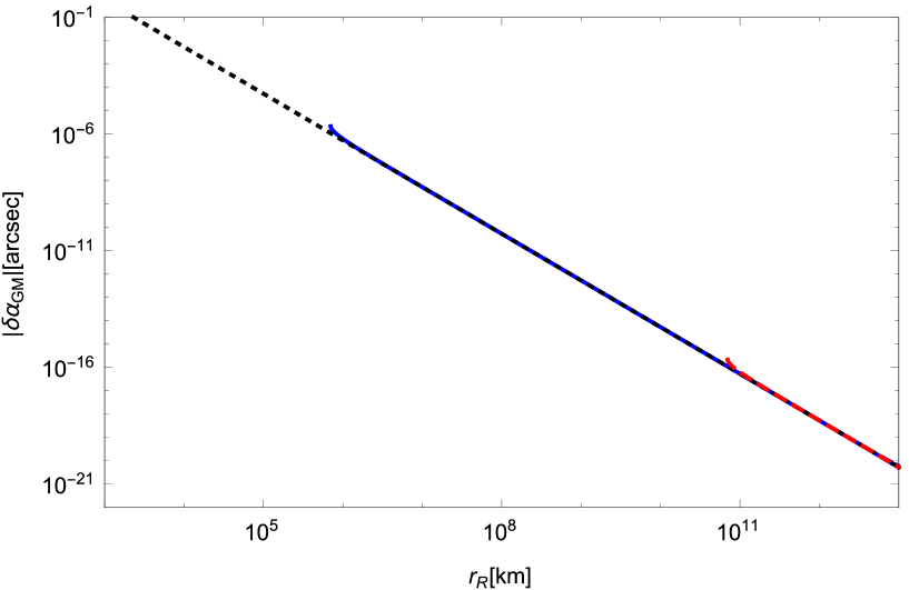
Figure 11: $\delta\alpha_{GM}$ for the Sun. The horizontal axis is the distance of the receiver distance $r_{R}$. The vertical axis means the finite-distance correction due to the gravitomagnetic deflection angle of light. The solid curve (blue in color) and dashed one (red in color) denote $b=R_{\odot}$ and $b=10^{5}R_{\odot}$, respectively. The dotted line (black in color) corresponds to the leading term in $\delta\alpha_{GM}$ given by Eq. (124). These three curves are overlapped. This implies the very weak dependence of $\delta\alpha_{GM}$ on $b$.

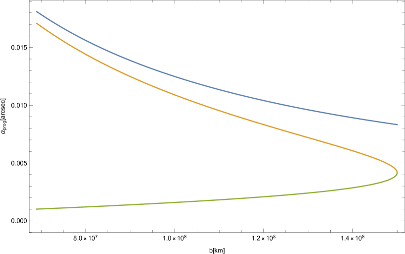
Figure 12: $\alpha$ in the prograde motion. The horizontal axis is the impact parameter for a photon orbit. The vertical axis means the deflection angle of light. The blue curve is the asymptotic deflection angle by a Kerr black hole. The orange curve means the deflection angle with finite-corrections by a Kerr black hole. The green curve shows the difference between the asymptotic bending angle and the deflection angle with finite-corrections by a Kerr black hole.

Figure 13: $\alpha$ for light of retrograde motion. The horizontal axis denotes the impact parameter for a photon orbit and the vertical axis denotes the deflection angle of light. The blue curve is the asymptotic deflection angle by the Kerr black hole. The orange curve is the deflection angle with finite-correction by the Kerr black hole. The green curve shows the difference between the asymptotic bending angle and the deflection angle with finite-correction by the Kerr black hole.

IX Rotating Teo wormhole: Another example

IX.1 Rotating Teo wormhole and optical metric

In this section, we consider a rotating Teo wormhole Teo in order to examine how our method can be applied to a wormhole spacetime. The spacetime metric for this wormhole is

$$ds^{2}= -N^{2}dt^{2}+\frac{dr^{2}}{1-\frac{b_{0}}{r}}+r^{2}H^{2}\Big{[}d\theta^{2}+\sin^{2}\theta(d\phi-\omega dt)^{2}\Big{]},$$ (128)

where we denote

$$N= H=1+\frac{d(4\bar{a}\cos\theta)^{2}}{r},$$ (129)

$$\omega= \frac{2\bar{a}}{r^{3}}.$$ (130)

Here, $b_{0}$ means the throat radius of this wormhole, $\bar{a}$ is corresponding to the spin angular momentum, and $d$ is a positive constant.

For the rotating Teo wormhole Eq.(128), the components of the generalized optical metric are Ono2018

$$\gamma_{ij}dx^{i}dx^{j}= \frac{r^{7}}{(r-b_{0})\left(r^{4}-4\bar{a}^{2}\sin^{2}\theta\right)\left(16d\bar{a}^{2}\cos^{2}\theta+r\right)^{2}}dr^{2}$$

$$+\frac{r^{6}}{r^{4}-4\bar{a}^{2}\sin^{2}\theta}d\theta^{2}+\frac{r^{10}\sin^{2}\theta}{\left(r^{4}-4\bar{a}^{2}\sin^{2}\theta\right)^{2}}d\phi^{2}.$$ (131)

Here, $\gamma_{ij}$ is not the induced metric in the ADM formulation. The components of $\beta_{i}$ are obtained as

$$\beta_{i}dx^{i}= -\frac{2\bar{a}r^{3}\sin^{2}\theta}{r^{4}-4\bar{a}^{2}\sin^{2}\theta}d\phi.$$ (132)

In this section, we restrict ourselves within the equatorial plane, namely $\theta=\pi/2$. On the equatorial plane, the constant $d$ in the metric always vanish, because $d$ is always associated with $\cos\theta$.

We employ the same way for the Kerr case, we first derive the orbit equation on the equatorial plane from Eq.(77) as

$$\left(\frac{dr}{d\phi}\right)^{2}= -\frac{r^{5}(b_{0}-r)\left(4\bar{a}^{2}b^{2}-4\bar{a}br^{3}-b^{2}r^{4}+r^{6}\right)}{\left(-4\bar{a}^{2}b+2\bar{a}r^{3}+br^{4}\right)^{2}}$$

$$= \frac{r^{4}}{b^{2}}-r^{2}-\frac{{b_{0}}r^{3}}{b^{2}}+{b_{0}}r-\frac{4\bar{a}r^{3}}{b^{3}}+\frac{4\bar{a}b_{0}r^{2}}{b^{3}}+\mathcal{O}(\bar{a}^{2}/b^{2}),$$ (133)

where $b$ denotes the impact parameter of the light ray and we use the weak field and slow rotation approximations in the last line. There are no $b_{0}$ squared terms in the last line. The orbit equation thus becomes

$$\left(\frac{du}{d\phi}\right)^{2}= \frac{1}{b^{2}}-u^{2}-\frac{b_{0}u}{b^{2}}+b_{0}u^{3}-\frac{4\bar{a}u}{b^{3}}-\frac{4\bar{a}b_{0}u^{2}}{b^{3}}+\mathcal{O}(\bar{a}^{2}/b^{6}).$$ (134)

This equation is iteratively solved as

$$u=\frac{\sin\phi}{b}+\frac{\cos^{2}\phi}{2b^{2}}b_{0}-\frac{2}{b^{3}}\bar{a}+\mathcal{O}\left(\frac{{b_{0}}^{2}}{b^{3}},\frac{\bar{a}b_{0}}{b^{4}}\right).$$ (135)

Solving Eq.(135) for $\phi_{S}$ and $\phi_{R}$, we obtain $\phi_{S}$ and $\phi_{R}$ as

$$\phi_{S}= \arcsin(bu_{S})-\frac{b_{0}\sqrt{1-b^{2}{u_{S}}^{2}}}{2b}+\frac{2\bar{a}}{b^{2}\sqrt{1-b^{2}{u_{S}}^{2}}}+\mathcal{O}\left(\frac{{b_{0}}^{2}}{b^{2}},\frac{\bar{a}b_{0}}{b^{3}}\right),$$ (136)

$$\phi_{R}= \pi-\arcsin(bu_{R})+\frac{b_{0}\sqrt{1-b^{2}{u_{R}}^{2}}}{2b}-\frac{2\bar{a}}{b^{2}\sqrt{1-b^{2}{u_{R}}^{2}}}+\mathcal{O}\left(\frac{{b_{0}}^{2}}{b^{2}},\frac{\bar{a}b_{0}}{b^{3}}\right).$$ (137)

IX.2 Gaussian curvature

In the weak field approximation, the Gaussian curvature of the equatorial plane is

$$K= -\frac{b_{0}}{2r^{3}}-\frac{56\bar{a}^{2}}{r^{6}}+\mathcal{O}\left(\frac{\bar{a}^{2}b_{0}}{r^{7}},\frac{\bar{a}^{4}}{r^{10}}\right),$$ (138)

where $\bar{a}$ and $b_{0}$ play a role of book-keeping parameters in the weak field approximation. It is not surprising that this Gaussian curvature deviates from Eq. (26) in Jusufi and Övgün JO , because their Gaussian curvature describes a different surface that is defined with using the Randers-Finsler metric. The Randers-Finsler metric is quite different from our generalized optical metric $\gamma_{ij}$.

When we perform the surface integral of the Gaussian curvature in Eq. (88), we use Eq.(135) for a boundary of the integration domain. The surface integral of the Gaussian curvature in Eq. (88) is thus calculated as

$$-\iint_{{}^{\infty}_{R}{\square}^{\infty}_{S}}KdS= \int_{\phi_{S}}^{\phi_{R}}\int_{\infty}^{r(\phi)}\left(-\frac{b_{0}}{2r^{2}}\right)drd\phi+\mathcal{O}\left(\frac{{b_{0}}^{2}}{b^{2}},\frac{\bar{a}b_{0}}{b^{3}}\right)$$

$$= \frac{b_{0}}{2}\int_{\phi_{S}}^{\phi_{R}}\int_{0}^{\frac{\sin\phi}{b}+\frac{\cos^{2}\phi}{2b^{2}}b_{0}-\frac{2}{b^{3}}\bar{a}}dud\phi+\mathcal{O}\left(\frac{{b_{0}}^{2}}{b^{2}},\frac{\bar{a}b_{0}}{b^{3}}\right)$$

$$= \frac{b_{0}}{2}\int_{\phi_{S}}^{\phi_{R}}\Big{[}\frac{\sin\phi}{b}\Big{]}d\phi+\mathcal{O}\left(\frac{{b_{0}}^{2}}{b^{2}},\frac{\bar{a}b_{0}}{b^{3}}\right)$$

$$= \frac{b_{0}}{2}\Big{[}-\frac{\cos\phi}{b}\Big{]}_{\phi=\phi_{S}}^{\phi_{R}}+\mathcal{O}\left(\frac{{b_{0}}^{2}}{b^{2}},\frac{\bar{a}b_{0}}{b^{3}}\right)$$

$$= \frac{b_{0}}{2b}\left(\sqrt{1-b^{2}{u_{R}}^{2}}+\sqrt{1-b^{2}{u_{S}}^{2}}\right)+\mathcal{O}\left(\frac{{b_{0}}^{2}}{b^{2}},\frac{\bar{a}b_{0}}{b^{3}}\right),$$ (139)

where we use $\sin{\phi_{R}}=bu_{R}+\mathcal{O}(\bar{a}b^{-2},b_{0}b^{-1})$ and $\sin{\phi_{S}}=bu_{S}+\mathcal{O}(\bar{a}b^{-2},b_{0}b^{-1})$ by Eqs.(137) and (136) in the last line.

IX.3 Geodesic curvature of photon orbit

We study the geodesic curvature of the photon orbit on the equatorial plane in the stationary and axisymmetric spacetime by using the generalized optical metric. It generally becomes Ono2017

$$\kappa_{g}=-\sqrt{\frac{1}{\gamma\gamma^{\theta\theta}}}\beta_{\phi,r}.$$ (140)

In the Teo wormhole, this expression is rearranged as

$$\kappa_{g}= -\frac{2\bar{a}}{r^{3}}+\frac{\bar{a}b_{0}}{r^{4}}+\frac{\bar{a}{b_{0}}^{2}}{4r^{5}}+\frac{\bar{a}{b_{0}}^{3}}{8r^{6}}\ +\mathcal{O}\left(\frac{\bar{a}^{3}}{r^{7}},\frac{\bar{a}^{3}b_{0}}{r^{8}}\right).$$ (141)

We compute the path integral of the geodesic curvature of the photon orbit. The detailed calculations and result are

$$\int_{S}^{R}\kappa_{g}d\ell= \int^{S}_{~{}R}\frac{2\bar{a}}{r^{3}}d\ell+\mathcal{O}\left(\frac{{b_{0}}^{2}}{b^{2}},\frac{\bar{a}b_{0}}{b^{3}}\right)$$

$$= \int^{\pi/2-\phi_{S}}_{~{}\pi/2-\phi_{R}}\frac{2\bar{a}\cos\vartheta}{b^{2}}d\vartheta+\mathcal{O}\left(\frac{{b_{0}}^{2}}{b^{2}},\frac{\bar{a}b_{0}}{b^{3}}\right)$$

$$= \frac{2\bar{a}}{b^{2}}\left[\sin\left(\frac{\pi}{2}-\phi_{S}\right)-\sin\left(\frac{\pi}{2}-\phi_{R}\right)\right]+\mathcal{O}\left(\frac{{b_{0}}^{2}}{b^{2}},\frac{\bar{a}b_{0}}{b^{3}}\right)$$

$$= \frac{2\bar{a}}{b^{2}}\left(\sqrt{1-b^{2}{u_{S}}^{2}}+\sqrt{1-b^{2}{u_{R}}^{2}}\right)+\mathcal{O}\left(\frac{{b_{0}}^{2}}{b^{2}},\frac{\bar{a}b_{0}}{b^{3}}\right),$$ (142)

for the retrograde orbit of the photon. In the last line, we used $\sin{\phi_{R}}=bu_{R}+\mathcal{O}(\bar{a}b^{-2},b_{0}b^{-1})$ and $\sin{\phi_{S}}=bu_{S}+\mathcal{O}(\bar{a}b^{-2},b_{0}b^{-1})$ from Eq. (135). The above result becomes $4\bar{a}/b^{2}$, as $r_{R}\to\infty$ and $r_{S}\to\infty$. The sign of the right hand side in Eq. (142) is opposite, if the photon is in the prograde motion.

IX.4 $\phi_{RS}$ part

The rotating Teo wormhole is an asymptotically flat spacetime as seen from Eq.(128). Therefore, the integral of the geodesic curvature of the circular arc segment with an infinite radius can be expressed simply as $\phi_{RS}$. By using Eqs.(136) and (137), $\phi_{RS}$ is obtained as

$$\phi_{RS}= \phi_{R}-\phi_{S}$$

$$= \pi-\arcsin(bu_{R})-\arcsin(bu_{S})+\frac{b_{0}\sqrt{1-b^{2}{u_{R}}^{2}}}{2b}+\frac{b_{0}\sqrt{1-b^{2}{u_{S}}^{2}}}{2b}$$

$$-\frac{2\bar{a}}{b^{2}\sqrt{1-b^{2}{u_{R}}^{2}}}-\frac{2\bar{a}}{b^{2}\sqrt{1-b^{2}{u_{S}}^{2}}}+\mathcal{O}\left(\frac{{b_{0}}^{2}}{b^{2}},\frac{\bar{a}b_{0}}{b^{3}}\right).$$ (143)

IX.5 $\Psi$ parts

For the rotating Teo wormhole by Eq.(128), Eq.(85) is computed as

$$\sin\Psi_{R}= bu_{R}+2\bar{a}{u_{R}}^{2}-4\bar{a}^{2}b{u_{R}}^{5},$$ (144)

and Eq.(86) becomes

$$\sin(\pi-\Psi_{S})= bu_{S}+2\bar{a}{u_{S}}^{2}-4\bar{a}^{2}b{u_{S}}^{5},$$ (145)

where the slow rotation approximation is not needed. Therefore, we obtain $\Psi_{R}$ and $\Psi_{S}$ as

$$\Psi_{R}= \arcsin(b{u_{R}})+\frac{2\bar{a}{u_{R}}^{2}}{\sqrt{1-b^{2}{u_{R}}^{2}}}+\frac{2\bar{a}^{2}b{u_{R}}^{5}\left(2b^{2}{u_{R}}^{2}-1\right)}{\left(b^{2}{u_{R}}^{2}-1\right)^{3/2}}+\mathcal{O}(\bar{a}^{3}/b^{6}),$$ (146)

$$\pi-\Psi_{S}= \arcsin(b{u_{S}})+\frac{2\bar{a}{u_{S}}^{2}}{\sqrt{1-b^{2}{u_{S}}^{2}}}+\frac{2\bar{a}^{2}b{u_{S}}^{5}\left(2b^{2}{u_{S}}^{2}-1\right)}{\left(b^{2}{u_{S}}^{2}-1\right)^{3/2}}+\mathcal{O}(\bar{a}^{3}/b^{6}),$$ (147)

where we used the slow rotation approximation.

IX.6 Deflection angle of light

We combine Eqs. (139) and (142) to obtain the deflection angle of light in the prograde orbit as

$$\alpha_{\mbox{prog}}= \frac{b_{0}}{2b}\left(\sqrt{1-b^{2}{u_{R}}^{2}}+\sqrt{1-b^{2}{u_{S}}^{2}}\right)-\frac{2\bar{a}}{b^{2}}\left(\sqrt{1-b^{2}{u_{R}}^{2}}+\sqrt{1-b^{2}{u_{S}}^{2}}\right)$$

$$+\mathcal{O}\left(\frac{{b_{0}}^{2}}{b^{2}},\frac{\bar{a}b_{0}}{b^{3}}\right).$$ (148)

The deflection angle of the retrograde light is

$$\alpha_{\mbox{retro}}= \frac{b_{0}}{2b}\left(\sqrt{1-b^{2}{u_{R}}^{2}}+\sqrt{1-b^{2}{u_{S}}^{2}}\right)+\frac{2\bar{a}}{b^{2}}\left(\sqrt{1-b^{2}{u_{R}}^{2}}+\sqrt{1-b^{2}{u_{S}}^{2}}\right)$$

$$+\mathcal{O}\left(\frac{{b_{0}}^{2}}{b^{2}},\frac{\bar{a}b_{0}}{b^{3}}\right).$$ (149)

Next, by using Eqs. (143), (146) and (147), we obtain the deflection angle of the prograde light as

$$\alpha_{\mbox{prog}}= \pi-\arcsin(bu_{R})-\arcsin(bu_{S})+\frac{b_{0}\sqrt{1-b^{2}{u_{R}}^{2}}}{2b}+\frac{b_{0}\sqrt{1-b^{2}{u_{S}}^{2}}}{2b}$$

$$-\frac{2\bar{a}}{b^{2}\sqrt{1-b^{2}{u_{R}}^{2}}}-\frac{2\bar{a}}{b^{2}\sqrt{1-b^{2}{u_{S}}^{2}}}+\arcsin(b{u_{R}})+\frac{2\bar{a}{u_{R}}^{2}}{\sqrt{1-b^{2}{u_{R}}^{2}}}$$

$$-\pi+\arcsin(b{u_{S}})+\frac{2\bar{a}{u_{S}}^{2}}{\sqrt{1-b^{2}{u_{S}}^{2}}}+\mathcal{O}\left(\frac{{b_{0}}^{2}}{b^{2}},\frac{\bar{a}b_{0}}{b^{3}}\right)$$

$$= \frac{b_{0}}{2b}\left(\sqrt{1-b^{2}{u_{R}}^{2}}+\sqrt{1-b^{2}{u_{S}}^{2}}\right)-\frac{2\bar{a}}{b^{2}}\left(\sqrt{1-b^{2}{u_{R}}^{2}}+\sqrt{1-b^{2}{u_{S}}^{2}}\right)$$

$$+\mathcal{O}\left(\frac{{b_{0}}^{2}}{b^{2}},\frac{\bar{a}b_{0}}{b^{3}}\right).$$ (150)

The deflection angle of light in the retrograde orbit is

$$\alpha_{\mbox{retro}}= \frac{b_{0}}{2b}\left(\sqrt{1-b^{2}{u_{R}}^{2}}+\sqrt{1-b^{2}{u_{S}}^{2}}\right)+\frac{2\bar{a}}{b^{2}}\left(\sqrt{1-b^{2}{u_{R}}^{2}}+\sqrt{1-b^{2}{u_{S}}^{2}}\right)$$

$$+\mathcal{O}\left(\frac{{b_{0}}^{2}}{b^{2}},\frac{\bar{a}b_{0}}{b^{3}}\right).$$ (151)

The deflection of light in the prograde (retrograde) orbit is weaker (stronger) with increasing the angular momentum of the Teo wormhole. The reason is as follows. The local inertial frame in which the light travels at the light speed $c$ in general relativity moves faster (slower). Hence, the time-of-flight of light becomes shorter (longer). On the light propagation A similar explanation is done by using the dragging of the inertial frame also by Laguna and Wolsczan LW . They discussed the Shapiro time delay. The expression of the deflection angle of light by a rotating Teo wormhole is similar to that by Kerr black hole. This implies that it is hard to distinguish Kerr black hole from rotating Teo wormhole by the gravitational lens observations.

In Eqs.(150) and (151), the source and receiver can be located at finite distance from the wormhole. In the limit as $r_{R}\to\infty$ and $r_{S}\to\infty$, Eqs. (148) and (149) become

$$\alpha_{\mbox{prog}}\rightarrow\frac{b_{0}}{b}-\frac{4\bar{a}}{b^{2}}+\mathcal{O}\left(\frac{{b_{0}}^{2}}{b^{2}},\frac{\bar{a}b_{0}}{b^{3}}\right),$$

$$\alpha_{\mbox{retro}}\rightarrow\frac{b_{0}}{b}+\frac{4\bar{a}}{b^{2}}+\mathcal{O}\left(\frac{{b_{0}}^{2}}{b^{2}},\frac{\bar{a}b_{0}}{b^{3}}\right).$$ (152)

They are in complete agreement with Eqs. (39) and (56) in Jusufi and Övgün JO , where they restrict themselves within the asymptotic source and receiver ($r_{R}\to\infty$ and $r_{S}\to\infty$).

IX.7 Finite-distance corrections in the Teo wormhole spacetime

To be precise, we define the finite-distance correction to the deflection angle of light as the difference between the asymptotic deflection angle $\alpha_{\infty}$ and the deflection angle for the finite distance case. It is denoted as $\delta\alpha$.

We consider the following situation. An observer on the Earth sees the light deflected by the solar mass. The source o light is located in a practically asymptotic region. In other words, we choose $b_{0}=M_{\odot}$, $\bar{a}=J_{\odot}$, $r_{R}\sim 1.5\times 10^{8}$ km, $r_{S}\sim\infty$. See Figure 14 for the finite-distance correction due to the impact parameter $b$. In Figure 14, the green curve means the difference between the asymptotic bending angle and the deflection angle with finite-distance corrections, the blue curve denotes the asymptotic deflection angle and the orange curve is the deflection angle with finite-distance corrections by the rotating Teo wormhole. The deflection angle is decreased by the finite-distance correction. If the impact parameter $b$ increases, the finite-distance correction also increases.

See also Figure 15 for numerical calculations of the finite-distance correction due to the impact parameter $b$. In Figure 15, the blue curve is the deflection angle with finite-distance correction by a Kerr black hole and the red curve is the deflection angle with finite-correction by a rotating Teo wormhole. The deflection of light is stronger in a Kerr black hole case for the chosen values.

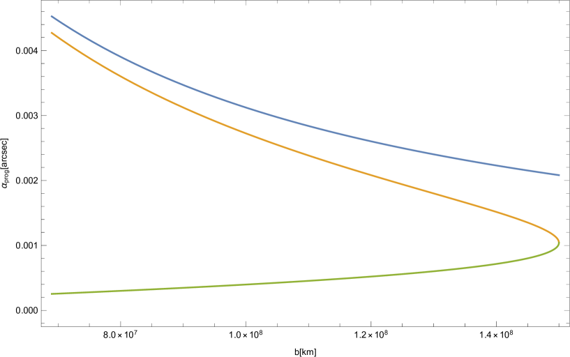
Figure 14: $\alpha$ in the Teo wormhole. The blue curve is the asymptotic deflection angle by the rotating Teo wormhole. The orange curve is the deflection angle with finite-distance corrections by the rotating Teo wormhole. The blue curve shows the difference between the asymptotic deflection angle and the deflection angle with finite-distance corrections by the rotating Teo wormhole.

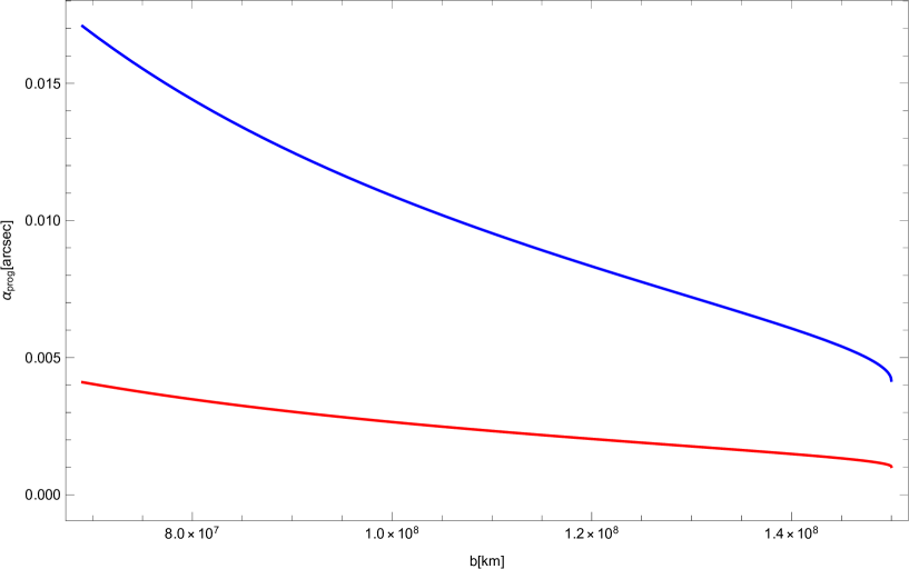
Figure 15: $\alpha$ for prograde motion of light. The horizontal axis is the impact parameter of photon orbit. The vertical axis means the deflection angle of light. The blue curve means the deflection angle with finite-distance corrections by the Kerr black hole. The red curve corresponds to that by the rotating Teo wormhole. For the purpose of this comparison, the mass of a Kerr black hole $M$ and the throat radius of a rotating Teo wormhole $b_{0}$ are chosen as $M=b_{0}=M_{\odot}$. The spin angular momentum of a Kerr black hole and that of a rotating Teo wormhole are chosen as the same as that the Sun for the simplicity.

X Summary

In this paper, we provided a brief review of a series of works on the deflection angle of light for a light source and receiver in a non-asymptotic region. Ishihara2016 ; Ishihara2017 ; Ono2017 ; Ono2018 . The validity and usefulness of the new formulation come from the GB theorem in differential geometry. First, we discussed how to define the gravitational deflection angle of light in a static, spherically symmetric and asymptotically flat spacetime, for which we assume the finite-distance source and receiver. We examined whether our definition is invariant geometrically by using the GB theorem. By using our definition, we carefully computed finite-distance corrections to the light deflection in Schwarzschild spacetime. We considered both cases of weak deflection and strong one. Next, we extended the definition to stationary and axisymmetric spacetimes. This extension allows us to compute finite-distance corrections for Kerr black holes and rotating Teo wormholes. We verified that these results are consistent with the previous works in the infinite-distance limit. We mentioned also the finite-distance corrections to the light deflection by Sagittarius A^∗. It is left as future work to apply the present formulation to other interesting spacetime models and also to extend it to a more general spacetime structure.

Appendix A Detailed calculations at $O(M^{2}/b^{2})$ and $O(a^{2}/b^{2})$ in Kerr spacetime

First, we investigate the Gaussian curvature $K$ of the equatorial plane in the Kerr spacetime. Here, we assume the weak field and slow rotation approximations. Up to the second order, $K$ is expanded as

$$K =\frac{R_{r\phi r\phi}}{\gamma}$$

$$=-\frac{2M}{r^{3}}+\frac{3M^{2}}{r^{4}}+O\left(\frac{a^{2}M}{r^{5}}\right),$$ (153)

where $\gamma$ denotes $\det{(\gamma_{ij})}$. There are no $a^{2}$ terms in $K$. More interestingly, only the $a^{2}M$ term at the third order level do exist in $K$. By noting that $K$ begins with $O(M)$, what we need for the second-order calculations is only the linear-order term in the area element on the equatorial plane. This is obtained as

$$dS\equiv \sqrt{\gamma}drd\phi$$

$$= \left[r+3M+O\left(\frac{M^{2}}{r}\right)\right]drd\phi,$$ (154)

where terms at $O(a)$ and also at $O(a^{2})$ do not exist in $dS$. This is because all terms including the spin parameter cancel out in $\gamma$ for $\theta=\pi/2$ and $\gamma$ thus depends only on $M$, as shown by direct calculations.

By using Eqs. (153) and (154), the surface integration of the Gaussian curvature is performed as

$$-\iint KdS= \int_{\infty}^{r_{OE}}dr\int_{\phi_{S}}^{\phi_{R}}d\phi\Big{(}-\frac{2M}{r^{3}}+\frac{3M^{2}}{r^{4}}\Big{)}(r+3M)+O\left(\frac{M^{3}}{b^{3}},\frac{aM^{2}}{b^{3}},\frac{a^{2}M}{b^{3}}\right)$$

$$= \int_{0}^{\frac{1}{b}\sin\phi+\frac{M}{b^{2}}(1+\cos^{2}\phi)}du\int_{\phi_{S}}^{\phi_{R}}d\phi~{}(2M+3uM^{2})+O\left(\frac{M^{3}}{b^{3}},\frac{aM^{2}}{b^{3}},\frac{a^{2}M}{b^{3}}\right)$$

$$= \int_{\phi_{S}}^{\phi_{R}}\Big{[}\frac{2M}{b}\sin\phi+\frac{M^{2}}{2b^{2}}(7+\cos^{2}\phi)\Big{]}d\phi+O\left(\frac{M^{3}}{b^{3}},\frac{aM^{2}}{b^{3}},\frac{a^{2}M}{b^{3}}\right)$$

$$= \frac{2M}{b}\Big{[}\cos\phi\Big{]}^{\phi_{S}}_{\phi_{R}}+\frac{M^{2}}{2b^{2}}\Big{[}\frac{30\phi+\sin(2\phi)}{4}\Big{]}^{\phi_{R}}_{\phi_{S}}+O\left(\frac{M^{3}}{b^{3}},\frac{aM^{2}}{b^{3}},\frac{a^{2}M}{b^{3}}\right)$$

$$= \frac{2M}{b}\Big{[}\sqrt{1-b^{2}{u_{S}}^{2}}+\sqrt{1-b^{2}{u_{R}}^{2}}\Big{]}$$

$$+\frac{15M^{2}}{4b^{2}}[\pi-\arcsin(bu_{S})-\arcsin(bu_{R})]$$

$$+\frac{M^{2}}{4b^{2}}[\frac{bu_{S}(15-7b^{2}{u_{S}}^{2})}{\sqrt{1-b^{2}{u_{S}}^{2}}}+\frac{bu_{R}(15-7b^{2}{u_{R}}^{2})}{\sqrt{1-b^{2}{u_{R}}^{2}}}]+O\left(\frac{M^{3}}{b^{3}},\frac{aM^{2}}{b^{3}},\frac{a^{2}M}{b^{3}}\right),$$ (155)

where we use, in the second line, an iterative solution for the orbit equation by Eq. (77) in the Kerr spacetime.

Next, we study the geodesic curvature. On the equatorial plane, we find

$$\kappa_{g}= -\frac{1}{\sqrt{\cfrac{\Sigma^{2}}{\Delta(\Sigma-2Mr)}\left(r^{2}+a^{2}+\cfrac{2a^{2}Mr\sin^{2}\theta}{\Sigma}\right)\cfrac{\Sigma\sin^{2}\theta}{(\Sigma-2Mr)}}}\beta_{\phi,r}$$

$$= -\frac{2aM}{r^{3}}+O\left(\frac{aM^{2}}{r^{3}}\right).$$ (156)

Note that $a^{2}$ terms do not exist. Therefore, we obtain

$$\int_{c_{p}}\kappa_{g}d\ell= -\int^{R}_{S}d\ell\left[\frac{2aM}{r^{2}}+O\left(\frac{aM^{2}}{r^{3}}\right)\right]$$

$$= -\frac{2aM}{b^{2}}\int^{\phi_{R}}_{~{}\phi_{S}}\cos\vartheta d\vartheta+O\left(\frac{aM^{2}}{b^{3}}\right)$$

$$= \frac{2aM}{b^{2}}[\sqrt{1-b^{2}{u_{R}}^{2}}+\sqrt{1-b^{2}{u_{S}}^{2}}]+O\left(\frac{aM^{2}}{b^{3}}\right),$$ (157)

where we use $\sin\phi_{S}=\sqrt{{r_{S}}^{2}-b^{2}}/r_{S}+O(M/r_{S})$ and $\sin\phi_{R}=-\sqrt{{r_{R}}^{2}-b^{2}}/r_{R}+O(M/r_{R})$.

By combining Eqs. (155) and (157), we obtain

$$\alpha\equiv -\iint_{{}^{\infty}_{R}\square^{\infty}_{S}}KdS-\int^{S}_{R}\kappa_{g}d\ell$$

$$= \frac{2M}{b}\Big{[}\sqrt{1-b^{2}{u_{S}}^{2}}+\sqrt{1-b^{2}{u_{R}}^{2}}\Big{]}$$

$$+\frac{15M^{2}}{4b^{2}}\left[\pi-\arcsin(bu_{S})-\arcsin(bu_{R})\right]$$

$$+\frac{M^{2}}{4b^{2}}\left[\frac{bu_{S}(15-7b^{2}{u_{S}}^{2})}{\sqrt{1-b^{2}{u_{S}}^{2}}}+\frac{bu_{R}(15-7b^{2}{u_{R}}^{2})}{\sqrt{1-b^{2}{u_{R}}^{2}}}\right]$$

$$-\frac{2aM}{b^{2}}\left[\sqrt{1-b^{2}{u_{R}}^{2}}+\sqrt{1-b^{2}{u_{S}}^{2}}\right]+O\left(\frac{M^{3}}{b^{3}},\frac{aM^{2}}{b^{3}},\frac{a^{2}M}{b^{3}}\right).$$ (158)

Note that $a^{2}$ terms and $a^{3}$ ones do not appear in $\alpha$ for the finite distance situation as well as in the infinite distance limit. If we assume the infinite distance limit $u_{R},u_{S}\to 0$, Eq. (158) becomes

$$\alpha\rightarrow\frac{4M}{b}+\frac{15\pi M^{2}}{4b^{2}}-\frac{4aM}{b^{2}}.$$ (159)

This agrees with the known results, especially on the numerical coefficients at the order of $M^{2}$ and $aM$.

References

• (1) A. Einstein, Ann. Phys. (Berlin) 49, 769 (1916).
• (2) F. W. Dyson, A. S. Eddington, C. Davidson, Phil. Trans. R. Soc. A 220, 291 (1920).
• (3) Y. Hagihara, Jpn. J Astron. Geophys. 8, 67 (1931).
• (4) S. Chandrasekhar, The Mathematical Theory of Black Holes, (Oxford University Press, New York, 1998).
• (5) C. W. Misner, K. S. Thorne, J. A. Wheeler, Gravitation, (Freeman, New York, 1973).
• (6) C. Darwin, Proc. R. Soc. A 249, 180 (1959).
• (7) V. Bozza, Phys. Rev. D 66, 103001 (2002).
• (8) S. V. Iyer and A. O. Petters, Gen. Relativ. Gravit. 39, 1563 (2007).
• (9) V. Bozza, and G. Scarpetta, Phys. Rev. D 76, 083008 (2007).
• (10) S. Frittelli, T. P. Kling, and E. T. Newman, Phys. Rev. D 61, 064021 (2000).
• (11) K. S. Virbhadra, and G. F. R. Ellis, Phys. Rev. D 62, 084003 (2000).
• (12) K. S. Virbhadra, Phys. Rev. D 79, 083004 (2009).
• (13) K. S. Virbhadra, D. Narasimha, and S. M. Chitre, Astron. Astrophys. 337, 1 (1998).
• (14) K. S. Virbhadra, and G. F. R. Ellis, Phys. Rev. D 65, 103004 (2002).
• (15) K. S. Virbhadra, and C. R. Keeton, Phys. Rev. D 77, 124014 (2008).
• (16) S. Zschocke, Class. Quantum Grav. 28, 125016 (2011).
• (17) E. F. Eiroa, G. E. Romero, and D. F. Torres, Phys. Rev. D 66, 024010 (2002).
• (18) V. Perlick, Phys. Rev. D 69, 064017 (2004).
• (19) F. Abe, Astrophys. J. 725, 787 (2010).
• (20) Y. Toki, T. Kitamura, H. Asada, and F. Abe, Astrophys. J. 740, 121 (2011).
• (21) K. Nakajima, and H. Asada, Phys. Rev. D 85, 107501 (2012).
• (22) G. W. Gibbons, and M. Vyska, Class. Quant. Grav. 29 065016 (2012).
• (23) J. P. DeAndrea, and K. M. Alexander, Phys. Rev. D 89, 123012 (2014).
• (24) T. Kitamura, K. Nakajima, and H. Asada, Phys. Rev. D 87, 027501 (2013).
• (25) N. Tsukamoto, and T. Harada, Phys. Rev. D 87, 024024 (2013).
• (26) K. Izumi, C. Hagiwara, K. Nakajima, T. Kitamura, and H. Asada, Phys. Rev. D 88, 024049 (2013).
• (27) T. Kitamura, K. Izumi, K. Nakajima, C. Hagiwara, and H. Asada, Phys. Rev. D 89, 084020 (2014).
• (28) K. Nakajima, K. Izumi, and H. Asada, Phys. Rev. D 90, 084026 (2014).
• (29) N. Tsukamoto, T. Kitamura, K. Nakajima, and H. Asada, Phys. Rev. D 90, 064043 (2014).
• (30) M. Azreg-Ainou, JCAP, 07, 037 (2015).
• (31) K. Akiyama et al. (Event Horizon Telescope Collaboration), Astrophys. J. 875, L1 (2019); Astrophys. J. 875, L2 (2019); Astrophys. J. 875, L3 (2019); Astrophys. J. 875, L4 (2019); Astrophys. J. 875, L5 (2019); Astrophys. J. 875, L6 (2019).
• (32) G. W. Gibbons, and M. C. Werner, Class. Quant. Grav. 25, 235009 (2008).
• (33) A. Ishihara, Y. Suzuki, T. Ono, T. Kitamura, and Hideki Asada, Phys. Rev. D 94, 084015 (2016).
• (34) A. Ishihara, Y. Suzuki, T. Ono, and Hideki Asada, Phys. Rev. D 95, 044017 (2017).
• (35) H. Arakida, Gen. Rel. Grav. 50, 48 (2018).
• (36) G. Crisnejo, E. Gallo, and A. Rogers, Phys. Rev. D 99, 124001 (2019).
• (37) T. Ono, A. Ishihara, and H. Asada, Phys. Rev. D 96, 104037 (2017).
• (38) T. Ono, A. Ishihara, and H. Asada, Phys. Rev. D 98, 044047 (2018).
• (39) A. Ovgun, Phys. Rev. D 98, 044033 (2018).
• (40) T. Ono, A. Ishihara, and H. Asada, Phys. Rev. D 99, 124030 (2019).
• (41) M. P. Do Carmo, Differential Geometry of Curves and Surfaces, pages 268-269, (Prentice-Hall, New Jersey, 1976).
• (42) F. Kottler, Annalen. Phys. 361, 401 (1918).
• (43) R. Bach, Math. Zeit. 9, 110 (1918).
• (44) R. J. Riegert, Phys. Rev. Lett. 53, 315 (1984).
• (45) P. D. Mannheim and D. Kazanas, Astrophys. J. 342, 635 (1989).
• (46) A. Edery, and M. B. Paranjape, Phys. Rev. D 58, 024011 (1998).
• (47) J. Sultana, and D. Kazanas, Phys. Rev. D 81, 127502 (2010).
• (48) C. Cattani, M. Scalia, E. Laserra, I. Bochicchio, and K. K. Nandi, Phys. Rev. D 87, 047503 (2013).
• (49) M. Sereno, Phys. Rev. Lett. 102, 021301 (2009).
• (50) A. Bhadra, S. Biswas, and K. Sarkar, Phys. Rev. D 82, 063003 (2010).
• (51) H. Arakida, and M. Kasai, Phys. Rev. D 85, 023006 (2012).
• (52) Y. Lim, and Q. Wang, Phys. Rev. D 95, 024004 (2017).
• (53) T. Lewis, Proc. Roy. Soc. A, 136, 176 (1932).
• (54) H. Levy, and W. J. Robinson, Proc. Camb. Phil. Soc. 60, 279 (1963).
• (55) A. Papapetrou, Ann. Inst. H. Poincare A, 4, 83 (1966).
• (56) In this paper, we use the polar coordinates. In the cylindrical coordinates, the line element is known as the Weyl-Lewis-Papapetrou form Lewis ; LR ; Papapetrou .
• (57) A. C. Belton, Geometry of Curves and Surfaces, page 38 (2015); www.maths.lancs.ac.uk/ belton/www/notes/geom notes.pdf; J. Oprea, Differential Geometry and Its Applications (2nd Edition), page 210, (Prentice Hall, New Jersey, 2003).
• (58) V. Perlick, Ray Optics, Fermat’s Principle, and Applications to General Relativity, (Springer, Berlin, 2000).
• (59) T. Levi-Civita, Absolute Differential Calculus, (Blackie and Son, Glasgow, 1927).
• (60) H. Asada, and M. Kasai, Prog. Theor. Phys. 104, 95 (2000).
• (61) M. C. Werner, Gen. Rel. Grav. 44, 3047 (2012).
• (62) S. Kopeikin, and B. Mashhoon, Phys. Rev. D 65, 064025 (2002).
• (63) R. Epstein, and I. I. Shapiro, Phys. Rev. D 22, 2947 (1980).
• (64) J. Ibanez, Astron. Astrophys. 124, 175 (1983).
• (65) S. V. Iyer, and E. C. Hansen, Phys. Rev. D 80, 124023 (2009).
• (66) G. V. Kraniotis, Class. Quant. Grav. 28, 085021 (2011).
• (67) Precise analytic treatments of the deflection angle of light were done in a conventional approach, on the equatorial plane of a Kerr black hole IH and for generic photon orbits in terms of the generalized hypergeometric functions of Appell and Lauricella Kraniotis . They assume that both the source and the receiver are located at the null infinity.
• (68) F. P. Pijpers, Mon. Not. Roy. Astron. Soc. 297, L76 (1998); S. L. Bi, T. D. Li, L. H. Li, and W. M. Yang, Astrophys. J. Lett. 731, L42 (2011).
• (69) http://sci.esa.int/gaia/
• (70) http://www.jasmine-galaxy.org/index-en.html
• (71) E. Teo, Phys. Rev. D 58, 024014 (1998).
• (72) K. Jusufi, and A. Övgün, Phys. Rev. D 97, 024042, (2018).
• (73) P. Laguna, A. Wolszczan, Astrophys. J., 486, L27 (1997).