Model independent analysis of New Physics effects on $B_{c}\to(D_{s},\,D^{\ast}_{s})\,\mu^{+}\mu^{-}$ decay observables

Abstract

Motivated by the anomalies present in $b\to s\,l^{+}\,l^{-}$ neutral current decays, we study the corresponding $B_{c}\to(D_{s},\,D^{\ast}_{s})\mu^{+}\mu^{-}$ decays within the standard model and beyond. We use a model independent effective theory formalism in the presence of vector and axial vector new physics operators and study the implications of the latest global fit to the $b\to s\,l^{+}\,l^{-}$ data on various observables for the $B_{c}\to(D_{s},\,D^{\ast}_{s})\mu^{+}\mu^{-}$ decays. We give predictions on several observables such as the differential branching ratio, ratio of branching ratios, forward backward asymmetry, and the longitudinal polarization fraction of the $D^{\ast}_{s}$ meson within standard model and within various new physics scenarios. These results can be tested at the Large Hadron Collider and, in principle, can provide complimentary information regarding new physics in $b\to s\,l^{+}\,l^{-}$ neutral current decays.

I Introduction

Although standard model (SM) of particle physics is successful in explaining various experimental observations, it, however, can not accommodate several long standing issues such as dark matter, dark energy, neutrino mass, matter antimatter asymmetry in the universe etc. It is indeed certain that physics beyond the SM exists. There are two ways to determine the nature of new physics (NP). One is direct detection of new particles and their interactions and another is indirect detection through their effects on various low energy processes. In this respect, flavor physics can, in principle, be the ideal platform to look for indirect evidences of NP. In fact, various anomalies with the SM prediction have been reported by dedicated experiments such as BABAR, Belle, and more recently by LHCb. In particular, measurement of various observables in $b\to c\tau\nu$ charged current interactions and in $b\to s\,l^{+}\,l^{-}$ neutral current interactions already provided hints of NP. We will focus here on anomalies present in $B$ meson decays mediated via $b\to s\,l^{+}\,l^{-}$ neutral current interactions. The most important observables are the lepton flavor universality (LFU) ratios $R_{K}$ and $R_{K^{\ast}}$, various angular observables in $B\to K^{\ast}\mu^{+}\mu^{-}$ decays, and the branching ratio of $B_{s}\to\phi\mu^{+}\mu^{-}$ decays. The experimental results confirming these anomalies are listed below.

A significant deviation from the SM expectation is observed in the LFU ratios $R_{K}$ and $R_{K^{\ast}}$ defined as

$$R_{K}^{(*)}=\frac{\mathcal{B}(B\to K^{(*)}\,\mu\mu)}{\mathcal{B}(B\to K^{(*)}\,e\,e)}\,.$$ (1)

The first LHCb measurement of $R_{K}=0.745^{+0.090}_{-0.074}\pm 0.036$ Aaij:2014ora in the low $q^{2}$ bin $1<q^{2}<6\,{\rm GeV^{2}}$ deviates from the SM prediction $R_{K}\approx 1$ Hiller:2003js ; Bobeth:2007dw ; Bordone:2016gaq at $2.6\sigma$ level. Very recently, the earlier measurement was superseded by LHCb Collaboration and it is reported to be $R_{K}=0.846^{+0.060+0.016}_{-0.054-0.014}$ Aaij:2019wad . Although it moves closer to the SM value, the deviation with the SM prediction still stands at $2.5\sigma$ level. Similarly, the measured value of $R_{K^{\ast}}=0.66^{+0.11}_{-0.07}\pm 0.03$ and $0.69^{+0.11}_{-0.07}\pm 0.05$ in the dilepton invariant mass $q^{2}=[0.045,\,1.1]\,{\rm GeV^{2}}$ and $[1.1,\,6.0]\,{\rm GeV^{2}}$ Aaij:2017vbb deviate from the SM prediction of $R_{K^{\ast}}\approx 1$ Capdevila:2016ivx ; Serra:2016ivr at approximately $2.1\sigma$ and $2.4\sigma$, respectively. Very recently, Belle collaboration has reported the values of $R_{K^{\ast}}$ in multiple $q^{2}$ bin but with a much larger uncertainties Abdesselam:2019wac . The other notable deviation is the deviation observed in the angular observable $P^{\prime}_{5}$ in $B\to K^{\ast}\mu^{+}\mu^{-}$ decays DescotesGenon:2012zf ; Descotes-Genon:2013vna . LHCb Aaij:2013qta ; Aaij:2015oid and ATLAS Aaboud:2018krd have measured the value of the angular observable $P^{\prime}_{5}$ in the $q^{2}$ range $4.0<q^{2}<6.0\,{\rm GeV^{2}}$ and the deviation from the SM prediction is found to be more than $3\sigma$ Aebischer:2018iyb . Belle Abdesselam:2016llu and CMS cms have also measured this observable in the $q^{2}$ bin $4.3<q^{2}<8.68\,{\rm GeV^{2}}$ and $4.3<q^{2}<6.0\,{\rm GeV^{2}}$, respectively. Although the Belle measured value differs from the SM expectation at $2.6\sigma$ level, the measured value by CMS is consistent with the SM expectation at $1\sigma$ level. Similarly, there is a systematic deficit in the measured value of branching ratio of $B_{s}\to\phi\mu^{+}\mu^{-}$ Aaij:2013aln ; Aaij:2015esa decays as compared to the SM prediction Aebischer:2018iyb ; Straub:2015ica . Currently the deviation with the SM prediction stands at around $3.7\sigma$. If it persists and is confirmed by future experiments, it could unravel new flavor structure beyond the SM physics. Various global fits Capdevila:2017bsm ; Altmannshofer:2017yso ; DAmico:2017mtc ; Hiller:2017bzc ; Geng:2017svp ; Ciuchini:2017mik ; Celis:2017doq ; Alok:2017sui ; Alok:2017jgr ; Alok:2019ufo to the $b\to s\,l^{+}\,l^{-}$ data have been performed and it was suggested that some of these anomalies can be resolved by modifying the Wilson coefficients (WCs).

If these anomalies are due to NP, this will show up in other $b\to s\,l^{+}\,l^{-}$ transition decays as well. In this paper, we analyze $B_{c}\to(D_{s},\,D^{\ast}_{s})\mu^{+}\mu^{-}$ decays mediated via $b\to s\,l^{+}\,l^{-}$ neutral current transitions within the SM and in several NP scenarios. LHCb has already measured the ratio of branching ratio $R_{J/\Psi}$ in $B_{c}\to J/\Psi\,l\,\nu$ decays. Detection and measurement of various observables pertaining to $B_{c}$ meson decaying to other mesons via $b\to s\,l^{+}\,l^{-}$ neutral current interactions will be feasible once more and more data will be accumulated by LHCb. It is worth mentioning that the study of such modes is complimentary to the study of $B\to(K,\,K^{\ast})\mu^{+}\mu^{-}$ decays and it can, in principle, provide useful information regarding different NP Lorentz structures. Moreover, study of these decay modes both theoretically and experimentally can act as a useful ingredient in maximizing future sensitivity to NP.

Within the SM, $B_{c}\to(D_{s},\,D^{\ast}_{s})\mu^{+}\mu^{-}$ decays have been studied previously using the relativistic constituent quark model Faessler:2002ut , light-front quark model Geng:2001vy ; Choi:2010ha , QCD sum rules Azizi:2008vy ; Azizi:2008vv , and relativistic quark model Ebert:2010dv . In this paper, we use the relativistic quark model of Ref. Ebert:2010dv and supplement the previous analysis by analyzing the effect of various NP on these decay modes in a model independent way. We use an effective theory formalism in the presence of new vector and axial vector couplings that couples only to the muon sector. We give prediction of various observables such as the ratio of branching ratios, lepton side forward backward asymmetry, and the longitudinal polarization fraction of the $D^{\ast}_{s}$ meson within the SM and within various NP scenarios.

Our paper is organized as follows. In section II, we start with the effective weak Hamiltonian for $b\to s\,l^{+}\,l^{-}$ decays in the presence of new vector and axial vector operators. We also discuss the hadronic matrix elements of $B_{c}\to D_{s}$ and $B_{c}\to D^{\ast}_{s}$ and their parametrization in terms of various meson to meson transition form factors. In section III, we write down the helicity amplitudes for the $B_{c}\to D_{s}\mu^{+}\mu^{-}$ and $B_{c}\to D^{\ast}_{s}\mu^{+}\mu^{-}$ decay modes and construct several observables. In section. IV, we give predictions of all the observables in the SM and in several NP cases obtained from the global fit. We conclude with a brief summary of our results in section. V.

II Formalism

The most general effective weak Hamiltonian in the presence of new vector and axial vector operators for the $|\Delta B|=|\Delta S|=1$ transition can be written as

$$\mathcal{H}_{\rm eff} = -\frac{4\,G_{F}}{\sqrt{2}}\,V_{tb}\,V_{ts}^{\ast}\,\frac{\alpha_{e}}{4\,\pi}\Big{[}C_{9}^{\rm eff}\bar{s}\gamma^{\mu}\,P_{L}\,b\,\bar{l}\gamma_{\mu}\,l+C_{10}\,\bar{s}\gamma^{\mu}\,P_{L}\,b\,\bar{l}\gamma_{\mu}\,\gamma_{5}\,l-\frac{2\,m_{b}}{q^{2}}\,C_{7}^{\rm eff}\,\bar{s}i\,q_{\nu}\,\sigma^{\mu\nu}\,P_{R}\,b\,\bar{l}\gamma_{\mu}\,l$$ (2)

$$+C_{9}^{NP}\,\bar{s}\gamma^{\mu}\,P_{L}\,b\,\bar{l}\gamma_{\mu}\,l+C_{10}^{NP}\,\bar{s}\gamma^{\mu}\,P_{L}\,b\,\bar{l}\gamma_{\mu}\,\gamma_{5}\,l+C^{\prime}_{9}\,\bar{s}\gamma^{\mu}\,P_{R}\,b\,\bar{l}\gamma_{\mu}\,l+C^{\prime}_{10}\,\bar{s}\gamma^{\mu}\,P_{R}\,b\,\bar{l}\gamma_{\mu}\,\gamma_{5}\,l\Big{]}\,,$$

where $G_{F}$ is the Fermi coupling constant, $\alpha_{e}$ is the electromagnetic coupling constant, $V_{tb}$ and $V_{ts}$ are the relevant Cabibbo Kobayashi Maskawa (CKM) matrix elements, and $P_{R,\,L}=(1\pm\gamma_{5})/2$ are the chiral projectors. All the WCs are evaluated at a renormalization scale of $\mu=m^{\rm pole}_{b}=4.8\,{\rm GeV}$. The $b$ quark mass associated with $C_{7}^{\rm eff}$ is considered to be running mass in the $\overline{\rm MS}$ scheme. In principle, there can be several NP Lorentz structures such as vector, axial vector, scalar, pseudoscalar, and tensor. The scalar, pseudoscalar and the tensor NP operators are severely constrained by $B_{s}\to\mu\mu$ and $b\to s\gamma$ measurements Alok:2010zd ; Alok:2011gv ; Bardhan:2017xcc . Hence, we consider NP in the form of vector and axial vector operators only. Again, we do not consider NP in the dipole operator as these are well constrained by radiative decays. The non factorizable corrections coming from electromagnetic corrections to the matrix elements of purely hadronic operators in the weak effective Hamiltonian are ignored in our analysis. These corrections, however, are expected to be significant at low $q^{2}$ Beneke:2001at ; Beneke:2004dp . All the NP WCs $C_{9}^{NP}$, $C_{10}^{NP}$, $C^{\prime}_{9}$, and $C^{\prime}_{10}$ are assumed to be real for our analysis. In the SM, $C_{9}^{NP}=C_{10}^{NP}=C^{\prime}_{9}=C^{\prime}_{10}=0$. The effective WCs $C_{7}^{\rm eff}$ and $C_{9}^{\rm eff}$ are defined as

$$C_{7}^{\rm eff}=C_{7}-\frac{1}{3}\,C_{5}-C_{6}\,,$$

$$C_{9}^{\rm eff}=C_{9}+y(q^{2})+y_{\rm BW}(q^{2})\,,$$ (3)

where the contributions coming from the one loop matrix elements of the four quark operators are contained in Buras:1994dj

$$y(q^{2}) = h\Big{(}\frac{m_{c}}{m_{b}},\,\frac{q^{2}}{m_{b}^{2}}\Big{)}(3\,C_{1}+C_{2}+3\,C_{3}+C_{4}+3\,C_{5}+C_{6})-\frac{1}{2}\,h\Big{(}1,\,\frac{q^{2}}{m_{b}^{2}}\Big{)}(4\,C_{3}+4\,C_{4}+3\,C_{5}+C_{6})$$ (4)

$$-\frac{1}{2}\,h\Big{(}0,\,\frac{q^{2}}{m_{b}^{2}}\Big{)}(C_{3}+3\,C_{4})+\frac{2}{9}(3\,C_{3}+C_{4}+3\,C_{5}+C_{6})\,.$$

Here

$$h(z,\,s)=-\ln\frac{m_{b}}{\mu}-\frac{8}{9}\ln\,z+\frac{8}{27}+\frac{4}{9}x-\frac{2}{9}(2+x)|1-x|^{1/2}\begin{cases}\ln\Big{|}\frac{\sqrt{1-x}+1}{\sqrt{1-x}-1}\Big{|}-i\,\pi&\rm{for}\,\,x=\frac{4\,z^{2}}{s}<1\\ 2\,\rm{arctan}\,\frac{1}{\sqrt{x-1}}&\rm{for}\,\,x=\frac{4\,z^{2}}{s}>1\end{cases}$$

$$h(0,\,s)=\frac{8}{27}-\ln\frac{m_{b}}{\mu}-\frac{4}{9}\ln\,s+\frac{4}{9}\,i\,\pi\,.$$ (5)

The phenomenological parameter $y_{\rm BW}(q^{2})$ involves the long distance effects coming from the $c\bar{c}$ resonance contributions coming from $J/\Psi$, $\Psi^{\prime}$ etc. In particular, these resonances provide large peaked contributions in the $q^{2}$ bins that are close to these charmonium resonance masses. The corresponding $q^{2}$ bins are not considered in our analysis. The values of masses of charm and bottom quark in these expressions are defined in pole mass scheme. The WCs that contains the short distance contribution can be calculated perturbatively, whereas, for the calculation of the long distance contributions contained in the matrix elements of local operators between initial and final hadron states, it requires non perturbative approach. The hadronic matrix elements can be expressed in terms of various meson to meson transition form factors.

The hadronic matrix elements for the $B_{c}\to D_{s}\mu^{+}\mu^{-}$ decays can be parametrized in terms of three invariant form factors. Those are

$$<D_{s}|\bar{s}\gamma^{\mu}b|B_{c}> = f_{+}(q^{2})\Big{[}p_{B_{c}}^{\mu}+p_{D_{s}}^{\mu}-\frac{M_{B_{c}}^{2}-M_{D_{s}}^{2}}{q^{2}}\,q^{\mu}\Big{]}+f_{0}(q^{2})\frac{M_{B_{c}}^{2}-M_{D_{s}}^{2}}{q^{2}}\,q^{\mu}\,,$$

$$<D_{s}|\bar{s}\sigma^{\mu\nu}\,q_{\nu}b|B_{c}> = \frac{i\,f_{T}(q^{2})}{M_{B_{c}}+M_{D_{s}}}\Big{[}q^{2}(p_{B_{c}}^{\mu}+p_{D_{s}}^{\mu}-(M_{B_{c}}^{2}-M_{D_{s}}^{2})q^{\mu}\Big{]}\,.$$ (6)

Similarly, for the $B_{c}\to D^{\ast}_{s}\mu^{+}\mu^{-}$ decays, the hadronic matrix elements can be parametrized in terms of seven invariant form factors, i.e,

$$<D^{\ast}_{s}|\bar{s}\gamma^{\mu}b|B_{c}> = \frac{2\,i\,V(q^{2})}{M_{B_{c}}+M_{D^{\ast}_{s}}}\,\epsilon^{\mu\nu\rho\sigma}\epsilon^{\ast}_{\nu}\,p_{B_{c_{\rho}}}\,p_{{D^{\ast}_{s}}_{\sigma}}\,,$$

$$<D^{\ast}_{s}|\bar{s}\gamma^{\mu}\gamma_{5}\,b|B_{c}> = 2\,M_{D^{\ast}_{s}}\,A_{0}(q^{2})\frac{\epsilon^{\ast}\cdot q}{q^{2}}\,q^{\mu}+(M_{B_{c}}+M_{D^{\ast}_{s}})\,A_{1}(q^{2})\Big{(}\epsilon^{{\ast}^{\mu}}-\frac{\epsilon^{\ast}\cdot q}{q^{2}}\,q^{\mu}\Big{)}\,$$

$$-A_{2}(q^{2})\frac{\epsilon^{\ast}\cdot q}{M_{B_{c}}+M_{D^{\ast}_{s}}}\,\Big{[}p_{B_{c}}^{\mu}+p_{D^{\ast}_{s}}^{\mu}-\frac{M_{B_{c}}^{2}-M_{D^{\ast}_{s}}^{2}}{q^{2}}\,q^{\mu}\Big{]}\,,$$

$$<D^{\ast}_{s}|\bar{s}\,i\,\sigma^{\mu\nu}\,q_{\nu}b|B_{c}> = 2\,T_{1}(q^{2})\,\epsilon^{\mu\nu\rho\sigma}\epsilon^{\ast}_{\nu}\,p_{B_{c_{\rho}}}\,p_{{D^{\ast}_{s}}_{\sigma}}\,,$$

$$<D^{\ast}_{s}|\bar{s}\,i\,\sigma^{\mu\nu}\,\gamma_{5}\,q_{\nu}b|B_{c}> = T_{2}(q^{2})\,\Big{[}(M_{B_{c}}^{2}-M_{D^{\ast}_{s}}^{2})\epsilon^{{\ast}^{\mu}}-(\epsilon^{\ast}\cdot q)(p_{B_{c}}^{\mu}+p_{D^{\ast}_{s}}^{\mu})\Big{]}$$ (7)

$$+T_{3}(q^{2})\,(\epsilon^{\ast}\cdot q)\Big{[}q^{\mu}-\frac{q^{2}}{M_{B_{c}}^{2}-M_{D^{\ast}_{s}}^{2}}(p_{B_{c}}^{\mu}+p_{D^{\ast}_{s}}^{\mu})\Big{]}\,,$$

where $q^{\mu}=(p_{B}-p_{D_{s},\,D^{\ast}_{s}})^{\mu}$ is the four momentum transfer and $\epsilon_{\mu}$ is polarization vector of the $D^{\ast}_{s}$ meson. For the $B_{c}\to D_{s}$ and $B_{c}\to D^{\ast}_{s}$ transition form factors we follow the relativistic quark model adopted in Ref. Ebert:2010dv . It was mentioned in Ref. Ebert:2010dv that in the limit of infinitely heavy quark mass and large energy of the final meson, the form factor results obtained in this approach are consistent with all the model independent symmetry relations Charles:1998dr ; Ebert:2001pc . We refer to Ref. Ebert:2010dv for all the omitted details.

III Helicity amplitudes and decay observables

For the helicity amplitudes, we pattern our analysis after that of Ref. Ebert:2010dv and, indeed, adopt a common notation. We use the helicity techniques of Refs. Korner:1989qb ; Kadeer:2005aq and write the hadronic helicity amplitudes for $B_{c}\to D_{s}\,l^{+}\,l^{-}$ decays in the presence of vector and axial vector NP operators as follows:

$$H_{\pm}^{(i)}=0\,,$$

$$H_{0}^{(1)}=\sqrt{\frac{\lambda}{q2}}\Big{[}(C_{9}^{\rm eff}+C_{9}^{NP}+C^{\prime}_{9})\,f_{+}(q^{2})+C_{7}^{\rm eff}\,\frac{2\,m_{b}}{M_{B_{c}}+M_{D_{s}}}\,f_{T}(q^{2})\Big{]}\,$$

$$H_{0}^{(2)}=\sqrt{\frac{\lambda}{q2}}\,(C_{10}+C_{10}^{NP}+C^{\prime}_{10})\,f_{+}(q^{2})\,,$$

$$H_{t}^{(1)}=\frac{M_{B_{c}}^{2}-M_{D_{s}}^{2}}{q^{2}}\,(C_{9}^{\rm eff}+C_{9}^{NP}+C^{\prime}_{9})\,f_{0}(q^{2})\,,$$

$$H_{t}^{(2)}=\frac{M_{B_{c}}^{2}-M_{D_{s}}^{2}}{q^{2}}\,(C_{10}+C_{10}^{NP}+C^{\prime}_{10})\,f_{0}(q^{2})\,$$ (8)

Similarly, for $B_{c}\to D^{\ast}_{s}\,l^{+}\,l^{-}$ decays, the hadronic helicity amplitudes are

$$H_{\pm}^{(1)} = -(M_{B_{c}}^{2}-M_{D^{\ast}_{s}}^{2})\Big{[}(C_{9}^{\rm eff}+C_{9}^{NP}-C^{\prime}_{9})\,\frac{A_{1}(q^{2})}{M_{B_{c}}-M_{D^{\ast}_{s}}}+\frac{2\,m_{b}}{q^{2}}\,C_{7}^{\rm eff}\,T_{2}(q^{2})\Big{]}$$

$$\pm\sqrt{\lambda}\Big{[}(C_{9}^{\rm eff}+C_{9}^{NP}+C^{\prime}_{9})\,\frac{V(q^{2})}{M_{B_{c}}+M_{D^{\ast}_{s}}}+\frac{2\,m_{b}}{q^{2}}\,C_{7}^{\rm eff}\,T_{2}(q^{2})\Big{]}\,,$$

$$H_{\pm}^{(2)} = (C_{10}+C_{10}^{NP}-C^{\prime}_{10})\Big{[}-(M_{B_{c}}+M_{D^{\ast}_{s}})\,A_{1}(q^{2})\Big{]}\pm(C_{10}+C_{10}^{NP}+C^{\prime}_{10})\frac{\lambda}{M_{B_{c}}+M_{D^{\ast}_{s}}}\,V(q^{2})\,,$$

$$H_{0}^{(1)} = -\frac{1}{2\,M_{D^{\ast}_{s}}\,\sqrt{q^{2}}}\Bigg{\{}(C_{9}^{\rm eff}+C_{9}^{NP}-C^{\prime}_{9})\,\Bigg{[}(M_{B_{c}}^{2}-M_{D^{\ast}_{s}}^{2}-q^{2})\,(M_{B_{c}}+M_{D^{\ast}_{s}})A_{1}(q^{2})-\frac{\lambda}{M_{B_{c}}+M_{D^{\ast}_{s}}}\,A_{2}(q^{2})\Bigg{]}\,$$

$$+2\,m_{b}\,C_{7}^{\rm eff}\,\Bigg{[}(M_{B_{c}}^{2}+3\,M_{D^{\ast}_{s}}^{2}-q^{2})\,T_{2}(q^{2})-\frac{\lambda}{M_{B_{c}}^{2}-M_{D^{\ast}_{s}}^{2}}\,T_{3}(q^{2})\Bigg{]}\Bigg{\}}\,$$

$$H_{0}^{(2)} = -\frac{1}{2\,M_{D^{\ast}_{s}}\,\sqrt{q^{2}}}\,(C_{10}+C_{10}^{NP}-C^{\prime}_{10})\Bigg{[}(M_{B_{c}}^{2}-M_{D^{\ast}_{s}}^{2}-q^{2})\,(M_{B_{c}}+M_{D^{\ast}_{s}})A_{1}(q^{2})-\frac{\lambda}{M_{B_{c}}+M_{D^{\ast}_{s}}}\,A_{2}(q^{2})\Bigg{]}\,$$

$$H_{t}^{(1)} = -\sqrt{\frac{\lambda}{q^{2}}}\,(C_{9}^{\rm eff}+C_{9}^{NP}-C^{\prime}_{9})\,A_{0}(q^{2})\,,$$

$$H_{t}^{(2)} = -\sqrt{\frac{\lambda}{q^{2}}}\,(C_{10}+C_{10}^{NP}-C^{\prime}_{10})\,A_{0}(q^{2})\,,$$ (9)

where

$$\lambda = M_{B_{c}}^{4}+M_{D_{s},\,D^{\ast}_{s}}^{4}+q^{4}-2\,(M_{B_{c}}^{2}\,M_{D_{s},\,D^{\ast}_{s}}^{2}+M_{D_{s},\,D^{\ast}_{s}}^{2}\,q^{2}+M_{B_{c}}^{2}\,q^{2})$$ (10)

Using the helicity amplitudes, the three body $B_{c}\to D_{s}\,l^{+}\,l^{-}$ and $B_{c}\to D^{\ast}_{s}\,l^{+}\,l^{-}$ differential decay rate can be written as Ebert:2010dv

$$\frac{d\Gamma}{dq^{2}} = \frac{G_{F}^{2}}{(2\pi)^{3}}\,\Bigg{(}\frac{\alpha_{e}\,|V_{tb}\,V_{ts}^{\ast}|}{2\pi}\Bigg{)}^{2}\,\frac{\lambda^{1/2}\,q^{2}}{48\,M_{B_{c}}^{3}}\,\sqrt{1-\frac{4\,m_{l}^{2}}{q^{2}}}\Bigg{[}H^{(1)}H^{{\dagger}^{(1)}}\,\Big{(}1+\frac{4\,m_{l}^{2}}{q^{2}}\Big{)}+H^{(2)}H^{{\dagger}^{(2)}}\,\Big{(}1-\frac{4\,m_{l}^{2}}{q^{2}}\Big{)}\,$$ (11)

$$+\frac{2\,m_{l}^{2}}{q^{2}}\,3\,H_{t}^{(2)}H_{t}^{{\dagger}^{(2)}}\Bigg{]}\,,$$

where $m_{l}$ denotes the mass of lepton and

$$H^{(i)}H^{{\dagger}^{(i)}} = H_{+}^{(i)}H_{+}^{{\dagger}^{(i)}}+H_{-}^{(i)}H_{-}^{{\dagger}^{(i)}}+H_{0}^{(i)}H_{0}^{{\dagger}^{(i)}}\,.$$ (12)

We define the differential ratio of branching ratio as follows:

$$R_{D_{s},\,D^{\ast}_{s}}(q^{2})=\frac{d\Gamma/dq^{2}\,\Big{(}B_{c}\to(D_{s},\,D^{\ast}_{s})\mu^{+}\mu^{-}\Big{)}}{d\Gamma/dq^{2}\,\Big{(}B_{c}\to(D_{s},\,D^{\ast}_{s})e^{+}\,e^{-}\Big{)}}\,.$$ (13)

We also construct observables like the forward backward asymmetry of the lepton pair $A_{FB}$ and the longitudinal polarization fraction of the $D^{\ast}_{s}$ meson $F_{L}$ as a function of dilepton invariant mass $q^{2}$. The forward backward asymmetry $A_{FB}(q^{2})$ is given by  Ebert:2010dv

$$A_{FB}(q^{2}) = \frac{3}{4}\sqrt{1-\frac{4\,m_{l}^{2}}{q^{2}}}\Bigg{\{}\frac{{\rm Re}\Big{(}H_{+}^{(1)}H_{+}^{{\dagger}^{(2)}}\Big{)}-{\rm Re}\Big{(}H_{-}^{(1)}H_{-}^{{\dagger}^{(2)}}\Big{)}}{H^{(1)}H^{{\dagger}^{(1)}}\,\Big{(}1+\frac{4\,m_{l}^{2}}{q^{2}}\Big{)}+H^{(2)}H^{{\dagger}^{(2)}}\,\Big{(}1-\frac{4\,m_{l}^{2}}{q^{2}}\Big{)}+\frac{2\,m_{l}^{2}}{q^{2}}\,3\,H_{t}^{(2)}H_{t}^{{\dagger}^{(2)}}}\Bigg{\}}\,.$$ (14)

Similarly, the longitudinal polarization fraction of the $D^{\ast}_{s}$ meson can be written as Ebert:2010dv

$$F_{L}(q^{2}) = \frac{H_{0}^{(1)}H_{0}^{{\dagger}^{(1)}}\,\Big{(}1+\frac{4\,m_{l}^{2}}{q^{2}}\Big{)}+H_{0}^{(2)}H_{0}^{{\dagger}^{(2)}}\,\Big{(}1-\frac{4\,m_{l}^{2}}{q^{2}}\Big{)}+\frac{2\,m_{l}^{2}}{q^{2}}\,3\,H_{t}^{(2)}H_{t}^{{\dagger}^{(2)}}}{H^{(1)}H^{{\dagger}^{(1)}}\,\Big{(}1+\frac{4\,m_{l}^{2}}{q^{2}}\Big{)}+H^{(2)}H^{{\dagger}^{(2)}}\,\Big{(}1-\frac{4\,m_{l}^{2}}{q^{2}}\Big{)}+\frac{2\,m_{l}^{2}}{q^{2}}\,3\,H_{t}^{(2)}H_{t}^{{\dagger}^{(2)}}}$$ (15)

It should be noted that the forward backward asymmetry observable $A_{FB}(q^{2})$ for the $B_{c}\to D_{s}\mu^{+}\mu^{-}$ decay mode is zero in the SM as the helicity amplitudes $H_{\pm}^{i}=0$. It is worth mentioning that it can have a non zero value only if it receives contribution from scalar, pseudoscalar or tensor NP operators. Since we consider NP in vector and axial vector operators only, we do not discuss $A_{FB}(q^{2})$ for the $B_{c}\to D_{s}\mu^{+}\mu^{-}$ decay mode in section. IV.

IV Results and discussion

IV.1 Inputs

For definiteness, we first report all the inputs that are used for the computation of all the decay observables. We employ a renormalization scale of $\mu=4.8\,{\rm GeV}$ throughout our analysis. For the meson masses, we use $M_{B_{c}}=6.2751\,{\rm GeV}$, $M_{D_{s}}=1.968\,{\rm GeV}$, and $M_{D^{\ast}_{s}}=2.1122\,{\rm GeV}$, as given in Ref. Tanabashi:2018oca . For the lepton masses, we use $m_{e}=0.5109989461\times 10^{-3}\,{\rm GeV}$ and $m_{\mu}=0.1056583715\,{\rm GeV}$ from Ref. Tanabashi:2018oca . Similarly, the mean life time of $B_{c}$ meson and the Fermi coupling constant are taken to be $\tau_{B_{c}}=0.507\times 10^{-12}\,{\rm s}$ and $G_{F}=1.1663787\times 10^{-5}\,{\rm GeV^{-2}}$, as reported in Ref. Tanabashi:2018oca . For the quark masses, we use $m_{b}(\overline{\rm MS})=4.2\,{\rm GeV}$, $m_{c}(\overline{\rm MS})=1.28\,{\rm GeV}$, and $m_{b}^{\rm pole}=4.8\,{\rm GeV}$  Altmannshofer:2008dz . For the electromagnetic coupling constant, we use $\alpha_{e}^{-1}=133.28$. We use $|V_{tb}V_{ts}|=0.0401\pm 0.0010$ as given in Ref. Bona:2006ah . The WCs in our numerical estimates, taken from Refs. Ali:1999mm , are reported in Table. 1.

$C_{1}$	$C_{2}$	$C_{3}$	$C_{4}$	$C_{5}$	$C_{6}$	$C_{7}^{\rm eff}$	$C_{9}$	$C_{10}$
$-0.248$	$1.107$	$0.011$	$-0.026$	$0.007$	$-0.031$	$-0.313$	$4.344$	$-4.669$

Table 1: Wilson coefficients evaluated at renormalization scale of $\mu=4.8\,{\rm GeV}$ from Ref. Ali:1999mm .

A relativistic quark model based on quasipotential approach was adopted in Ref. Ebert:2010dv to determine various $B_{c}\to D_{s}$ and $B_{c}\to D^{\ast}_{s}$ transition form factors. Various form factors at $q^{2}=0$ and the fitted parameters $\sigma_{1}$ and $\sigma_{2}$, taken from Ref. Ebert:2010dv , are reported in Table. 2.

	$f_{+}$	$f_{0}$	$f_{T}$	$V$	$A_{0}$	$A_{1}$	$A_{2}$	$T_{1}$	$T_{2}$	$T_{3}$
$F_{0}$	$0.129$	$0.129$	$0.098$	$0.182$	$0.070$	$0.089$	$0.110$	$0.085$	$0.085$	$0.051$
$\sigma_{1}$	$2.096$	$2.331$	$1.412$	$2.133$	$1.561$	$2.479$	$2.833$	$1.540$	$2.577$	$2.783$
$\sigma_{2}$	$1.147$	$1.666$	$0.048$	$1.183$	$0.192$	$1.686$	$2.167$	$0.248$	$1.859$	$2.170$

Table 2: $B_{c}\to D_{s}$ and $B_{c}\to D^{\ast}_{s}$ form factors at $q^{2}=0$ and the fitted parameters $\sigma_{1}$ and $\sigma_{2}$ from Ref. Ebert:2010dv .

It was shown in Ref. Ebert:2010dv that the $q^{2}$ dependence of the form factors can be well parametrized and reproduced in the form:

$$F(q^{2}) = \frac{F(0)}{\Big{(}1-\frac{q^{2}}{M^{2}}\Big{)}\Big{(}1-\sigma_{1}\,\frac{q^{2}}{M_{B^{\ast}_{s}}^{2}}+\sigma_{2}\,\frac{q^{4}}{M_{B^{\ast}_{s}}^{4}}\Big{)}}$$ (16)

for $F(q^{2})=f_{+}(q^{2}),\,f_{T}(q^{2}),\,V(q^{2}),\,A_{0}(q^{2}),\,T_{1}(q^{2})$. Whereas, for $F(q^{2})=f_{0}(q^{2}),\,A_{1}(q^{2}),\,A_{2}(q^{2}),\,T_{2}(q^{2}),\,T_{3}(q^{2})$, it can be well approximated by

$$F(q^{2}) = \frac{F(0)}{\Big{(}1-\sigma_{1}\,\frac{q^{2}}{M_{B^{\ast}_{s}}^{2}}+\sigma_{2}\,\frac{q^{4}}{M_{B^{\ast}_{s}}^{4}}\Big{)}}\,,$$ (17)

where $M=M_{B_{s}}$ for $A_{0}(q^{2})$ and $M=M_{B^{\ast}_{s}}$ for all other form factors. We use $M_{B_{s}}=5.36689\,{\rm GeV}$ and $M_{B^{\ast}_{s}}=5.4154\,{\rm GeV}$ from Ref. Tanabashi:2018oca . The form factors describe the hadronisation of quarks and gluons: these involve QCD in the non-perturbative regime and are a significant source of theoretical uncertainties. To gauge the effect of the form factor uncertainties on various observables, we have used $\pm 5\%$ uncertainty in $F(0)$, $\sigma_{1}$ and $\sigma_{2}$.

IV.2 SM prediction of $B_{c}\to(D_{s},\,D^{\ast}_{s})\,l\,\bar{l}$ decay observables

Now let us proceed to discuss our results in the SM. In Table. 3, we report our $q^{2}$ bin averaged values of various observables for the $B_{c}\to D_{s}\,\mu^{+}\,\mu^{-}$ and $B_{c}\to D^{\ast}_{s}\,\mu^{+}\,\mu^{-}$ decays. We restrict our analysis to low dilepton invariant mass region and consider seven $q^{2}$ bins ranging from $(0.045-6.0)\,{\rm GeV^{2}}$. The central values are obtained using the central values of all the input parameters. For the uncertainties, we have performed a naive $\chi^{2}$ analysis defined as

$$\chi^{2}=\sum_{i}\,\frac{(\mathcal{O}_{i}-\mathcal{O}_{i}^{0})^{2}}{\Delta_{i}^{2}}\,,$$ (18)

where $\mathcal{O}_{i}=(|V_{tb}V_{ts}^{\ast}|,\,F(0),\,\sigma_{1},\,\sigma_{2})$. Here $\mathcal{O}_{i}^{0}$ represents the central values of all the parameters and $\Delta_{i}$ represents $1\sigma$ uncertainty associated with each parameter. To find out the uncertainties in each observable, We impose $\chi^{2}\leq 2.156$ for the $B_{c}\to D_{s}\,\mu^{+}\,\mu^{-}$ decays and $\chi^{2}\leq 8.643$ for the $B_{c}\to D^{\ast}_{s}\,\mu^{+}\,\mu^{-}$ decays.

Observable/$q^{2}$ bin	$[0.045-1.0]$	$[1.0-2.0]$	$[2.0-3.0]$	$[3.0-4.0]$	$[4.0-5.0]$	$[5.0-6.0]$	$[1.0-6.0]$
$10^{7}\times\mathcal{B}(B_{c}\to D_{s}\,\mu\mu)$	$0.025\pm 0.001$	$0.030\pm 0.002$	$0.034\pm 0.002$	$0.038\pm 0.002$	$0.043\pm 0.003$	$0.049\pm 0.004$	$0.194\pm 0.013$
$R_{D_{s}}$	$1.006\pm 0.008$	$1.007\pm 0.002$	$1.005\pm 0.001$	$1.004\pm 0.001$	$1.003\pm 0.001$	$1.003\pm 0.001$	$1.004\pm 0.001$
$10^{7}\times\mathcal{B}(B_{c}\to D^{\ast}_{s}\,\mu\mu)$	$0.024\pm 0.001$	$0.011\pm 0.001$	$0.014\pm 0.002$	$0.020\pm 0.002$	$0.028\pm 0.003$	$0.039\pm 0.004$	$0.113\pm 0.012$
$<A_{FB}^{D^{\ast}_{s}}>$	$-0.064\pm 0.002$	$-0.076\pm 0.012$	$0.033\pm 0.006$	$0.110\pm 0.009$	$0.160\pm 0.011$	$0.194\pm 0.013$	$0.123\pm 0.009$
$<F_{L}^{D^{\ast}_{s}}>$	$0.266\pm 0.033$	$0.711\pm 0.034$	$0.662\pm 0.032$	$0.566\pm 0.035$	$0.488\pm 0.036$	$0.430\pm 0.037$	$0.526\pm 0.035$
$R_{D^{\ast}_{s}}$	$0.999\pm 0.005$	$0.993\pm 0.002$	$0.992\pm 0.001$	$0.993\pm 0.001$	$0.994\pm 0.001$	$0.995\pm 0.001$	$0.994\pm 0.001$

Table 3: $q^{2}$ bin (in ${\rm GeV^{2}}$) averaged values of various observables of $B_{c}\to D_{s}\mu^{+}\mu^{-}$ and $B_{c}\to D^{\ast}_{s}\mu^{+}\mu^{-}$ decays in the SM. The uncertainties in each observable corresponds to the uncertainties associated with the meson to meson transition form factors and the CKM matrix elements.

In the SM, we find the branching ratios of $B_{c}\to(D_{s},\,D^{\ast}_{s})\mu^{+}\mu^{-}$ decays to be of $\mathcal{O}(10^{-8})$ which might be within the experimental sensitivity of LHCb because of the large number of $B_{c}$ meson that is being produced at the LHC. We also obtain the LFU ratios to be $R_{D_{s},\,D^{\ast}_{s}}\approx 1$ in the SM. It is observed that in the $q^{2}$ bin ranging from $(0.045-2)\,{\rm GeV^{2}}$, the $<A_{FB}^{D^{\ast}_{s}}>$ observable assumes negative values, whereas, for $q^{2}>2\,{\rm GeV^{2}}$, it assumes positive values. It should be noted that the uncertainty associated with the LFU ratios $R_{D_{s}}$ and $R_{D^{\ast}_{s}}$ are quite negligible in comparison to the uncertainties present in the branching ratio, the forward backward asymmetry $<A_{FB}^{D^{\ast}_{s}}>$ and the longitudinal polarization fraction of the $D^{\ast}_{s}$ meson $<F_{L}^{D^{\ast}_{s}}>$. Measurements of these ratios in future will be crucial in determining various NP Lorentz structures.

We have shown in Fig. 1 the $q^{2}$ dependence of differential branching ratios, forward backward asymmetry, and longitudinal polarization fraction of $D^{\ast}_{s}$ meson in the low $q^{2}$ region $0.045\leq q^{2}\leq 6\,{\rm GeV^{2}}$. The line corresponds to the central values of all the input parameters, whereas, the band corresponds to the uncertainties associated with the CKM matrix element and the form factor inputs. In the SM, we find the zero crossing in $A_{FB}(q^{2})$ of $B_{c}\to D^{\ast}_{s}\mu^{+}\mu^{-}$ decays at $q^{2}=2.2\,{\rm GeV^{2}}$. Our results are quite similar to the values reported in Ref. Ebert:2010dv . Slight deviations may occur due to different choices of input parameters.

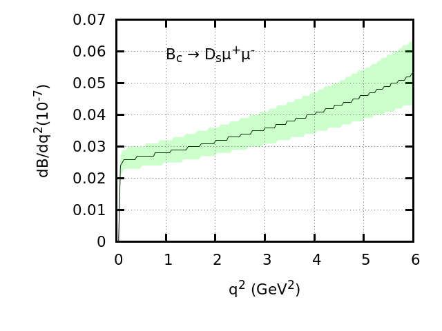
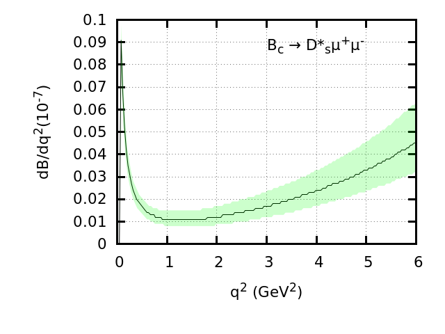
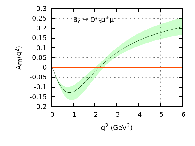
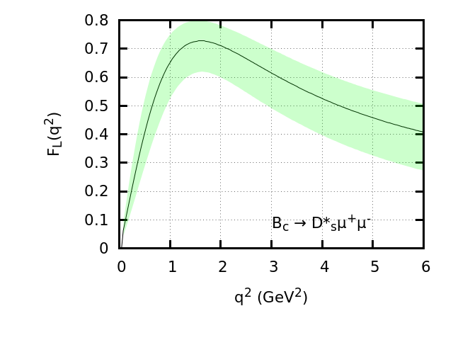
Figure 1: Differential branching ratio $d\mathcal{B}/dq^{2}$, forward backward asymmetry of lepton pair $A_{FB}(q^{2})$ and longitudinal polarization fraction of $D^{\ast}_{s}$ meson $F_{L}(q^{2})$ for the $B_{c}\to D_{s}\mu^{+}\mu^{-}$ and $B_{c}\to D^{\ast}_{s}\mu^{+}\mu^{-}$ decays in the SM. The band corresponds to the uncertainties in the transition form factors and the CKM matrix elements as discussed in the text.

IV.3 New Physics analysis

Our main objective is to determine the effect of NP on $B_{c}\to(D_{s},\,D^{\ast}_{s})\mu^{+}\,\mu^{-}$ decay observables in a model independent way. To this end, we use an effective theory formalism in the presence of new vector (V) and axial vector (A) couplings in our analysis. Although there can be other NP Lorentz structures such as scalar (S), pseudoscalar (P) and tensor (T), they are severely constrained by $B_{s}\to\mu\mu$ and $b\to s\gamma$ data. Hence we omit any discussion regarding these NP operators. Global fits of NP to the $b\to s\,l^{+}\,l^{-}$ data have been carried out by several groups Capdevila:2017bsm ; Altmannshofer:2017yso ; DAmico:2017mtc ; Hiller:2017bzc ; Geng:2017svp ; Ciuchini:2017mik ; Celis:2017doq ; Alok:2017sui ; Alok:2017jgr ; Alok:2019ufo . In Ref. Alok:2019ufo , the authors perform a global fit of $C_{9}^{NP}$, $C_{10}^{NP}$, $C^{\prime}_{9}$, and $C^{\prime}_{10}$ by using the constraints coming not only from $R_{K}$, $R_{K^{\ast}}$, $P^{\prime}_{5}$, and $\mathcal{B}(B_{s}\to\phi\mu^{+}\mu^{-})$ but also from $\mathcal{B}(B_{s}\to\mu^{+}\mu^{-})$, differential branching ratios of $B^{0,\,+}\to K^{{0,\,+}^{\ast}}\mu^{+}\mu^{-}$, $B^{0,\,+}\to K^{0,\,+}\mu^{+}\mu^{-}$ and $B\to X_{s}\mu^{+}\mu^{-}$, angular observables in $B^{0}\to K^{0^{\ast}}\mu^{+}\mu^{-}$ and $B_{s}\to\phi\mu^{+}\mu^{-}$ decays. Two different scenarios were considered in Ref. Alok:2019ufo . In $1D$ scenario, the best solutions to these anomalies were obtained for $C_{9}^{NP}$, $C_{10}^{NP}$, $C_{9}^{NP}=-C_{10}^{NP}$ and $C_{9}^{NP}=-C^{\prime}_{9}$. Similarly, for $2D$ scenario, where NP contributes to two WCs, the best solutions were obtained for $(C_{9}^{NP},\,C_{10}^{NP})$, $(C_{9}^{NP},\,C^{\prime}_{9})$, and $(C_{9}^{NP},\,C^{\prime}_{10})$. There are other possibilities with different WCs exist that give rise to similar fits. We, however, consider only seven of them: four from $1D$ scenario and three from $2D$ scenario. The best fit values and the corresponding $\Delta\chi^{2}$ values of all these NP WCs for $1D$ and $2D$ scenarios, taken from Ref. Alok:2019ufo , are reported in Table. 4. It should be noted that NP contributions to $(C_{9}^{NP},\,C^{\prime}_{9})$ and $(C_{9}^{NP},\,C^{\prime}_{10})$ are the most favored ones from the $2D$ scenario and NP in $C_{9}^{NP}=-C^{\prime}_{9}$ is the most favored one from $1D$ scenario.

Wilson coefficients	Best fit values	$\Delta\chi^{2}$
$C_{9}^{NP}$	$-1.07$	$37.6$
$C_{10}^{NP}$	$+0.78$	$27.0$
$C_{9}^{NP}=-C_{10}^{NP}$	$-0.52$	$36.3$
$C_{9}^{NP}=-C_{9}^{\prime}$	$-1.11$	$40.5$
$(C_{9}^{NP},\,C_{10}^{NP})$	$(-0.94,\,+0.23)$	$41.8$
$(C_{9}^{NP},\,C_{9}^{\prime})$	$(-1.27,\,+0.68)$	$49.4$
$(C_{9}^{NP},\,C_{10}^{\prime})$	$(-1.36,\,-0.46)$	$52.8$

Table 4: Best fit and the corresponding $\Delta\chi^{2}$ values of different new vector and axial vector Wilson coefficients in $1D$ and $2D$ scenarios taken from Ref. Alok:2019ufo .

In Appendix A, we report $q^{2}$ bin averaged values of various observables such as the branching ratio, ratio of branching ratio, forward backward asymmetry, and longitudinal polarization fraction of the $D^{\ast}_{s}$ meson for the $B_{c}\to D_{s}\mu^{+}\mu^{-}$ and $B_{c}\to D^{\ast}_{s}\mu^{+}\mu^{-}$ decays in the presence of these NP WCs. In each $q^{2}$ bin, the branching ratio of $B_{c}\to D_{s}\mu^{+}\mu^{-}$ is smaller in each NP scenarios than in the SM except for $C_{9}^{NP}=-C^{\prime}_{9}$. It remains SM like for $C_{9}^{NP}=-C^{\prime}_{9}$. Similar conclusion can be made for the ratio of branching ratio $R_{D_{s}}$ as well. For the $B_{c}\to D^{\ast}_{s}\mu^{+}\mu^{-}$ decay, the bin averaged branching ratio and the ratio of branching ratio $R_{D^{\ast}_{s}}$ in each $q^{2}$ bin for each NP scenarios are smaller than the corresponding SM value. However, the $A_{FB}$ and $F_{L}$ values can be either smaller or larger in NP cases than the SM central value. It should be mentioned that the deviation of $R_{D_{s}}$, $R_{D^{\ast}_{s}}$ and $A_{FB}$ from the SM prediction can be quite large in some $q^{2}$ bins.

In Fig. 2, we show various $q^{2}$ dependent observables for the $B_{c}\to(D_{s},\,D^{\ast}_{s})\mu^{+}\,\mu^{-}$ decays in the presence of various NP WCs in $1D$ scenario. Our observations are as follows:

• The differential branching ratio for the $B_{c}\to D_{s}\,\mu^{+}\,\mu^{-}$ decays is reduced at all $q^{2}$ for $C_{9}^{NP}$, $C_{10}^{NP}$, and $C_{9}^{NP}=-C_{10}^{NP}$, whereas, it remains SM like for $C_{9}^{NP}=-C^{\prime}_{9}$. This could very well be understood from Eq. III that $H_{0}^{(1)}$ and $H_{t}^{(1)}$ helicity amplitudes for the $B_{c}\to D_{s}\,\mu^{+}\,\mu^{-}$ decay mode depend on the combination $C_{9}^{NP}+C^{\prime}_{9}$. Hence the NP contribution cancels.

• The differential branching ratio for the $B_{c}\to D^{\ast}_{s}\,\mu^{+}\,\mu^{-}$ decays is reduced at all $q^{2}$ for $C_{9}^{NP}$, $C_{10}^{NP}$, $C_{9}^{NP}=-C_{10}^{NP}$, and $C_{9}^{NP}=-C^{\prime}_{9}$. The deviation with the SM prediction increases as $q^{2}$ increases for each NP WCs.

• For all the NP couplings, the zero crossing in the forward backward asymmetry observable $A_{FB}^{D^{\ast}_{s}}$ is shifted to the higher values of $q^{2}$ than in the SM. There is, however, one exception. For $C_{10}^{NP}=0.78$, the zero crossing coincides with the SM prediction although the shape of $A_{FB}^{D^{\ast}_{s}}$ may slightly vary. Maximum deviation from the SM prediction is observed for $C_{9}^{NP}$ and $C_{9}^{NP}=-C^{\prime}_{9}$.

• The peak of the longitudinal polarization fraction of $D^{\ast}_{s}$ meson may shift towards a higher values of $q^{2}$ than in the SM. Although the longitudinal polarization fraction $F_{L}$ is reduced at all $q^{2}$ for $C_{9}^{NP}$, $C_{9}^{NP}=-C_{10}^{NP}$, and $C_{9}^{NP}=-C^{\prime}_{9}$, it may increase with $C_{10}^{NP}$ for $q^{2}>1.2\,{\rm GeV^{2}}$.

There are other combinations of VA couplings exist in the $1D$ scenario as reported in Ref. Alok:2019ufo . We, however, do not consider those cases because of their small $\Delta\chi^{2}$ values.

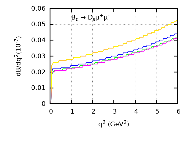
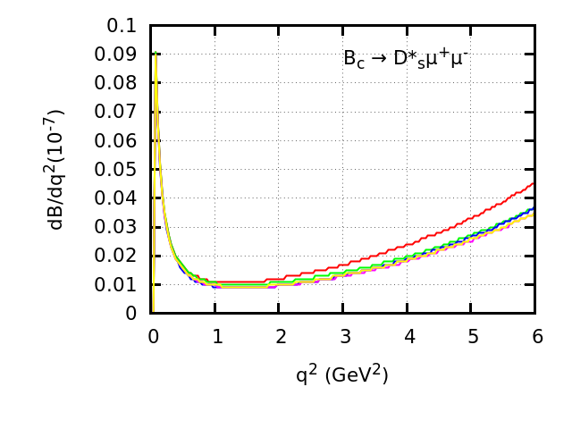
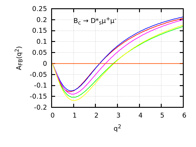
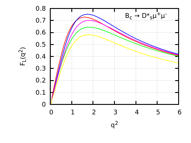
Figure 2: Differential branching ratio $d\mathcal{B}/dq^{2}$, forward backward asymmetry of lepton pair $A_{FB}(q^{2})$ and longitudinal polarization fraction of $D^{\ast}_{s}$ meson $F_{L}(q^{2})$ for the $B_{c}\to D_{s}\mu^{+}\mu^{-}$ and $B_{c}\to D^{\ast}_{s}\mu^{+}\mu^{-}$ decays in the SM (Red) and for the best fit values of new VA couplings in $1D$ scenario. Green, blue, purple, and yellow lines correspond to the best fit values of $C_{9}^{NP}=-1.07$, $C_{10}^{NP}=0.78$, $C_{9}^{NP}=-C_{10}^{NP}=-0.52$, and $C_{9}^{NP}=-C^{\prime}_{9}=-1.11$, respectively.

We now consider several NP couplings from the $2D$ scenarios having high $\Delta\chi^{2}$ values from the global fit Alok:2019ufo . The best fit values, taken from Ref. Alok:2019ufo , are reported in table. 4. We show in Fig. 3 various observables such as Differential branching ratio $d\mathcal{B}/dq^{2}$, forward backward asymmetry of lepton pair $A_{FB}(q^{2})$ and longitudinal polarization fraction of $D^{\ast}_{s}$ meson $F_{L}(q^{2})$ as a function of dilepton invariant mass $q^{2}$ for the $B_{c}\to D_{s}\mu^{+}\mu^{-}$ and $B_{c}\to D^{\ast}_{s}\mu^{+}\mu^{-}$ decays in the presence of such NP. Our main observations are as follows:

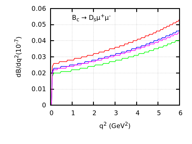
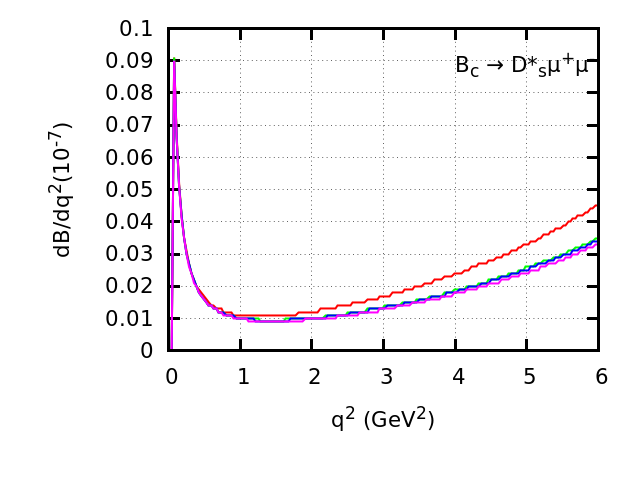
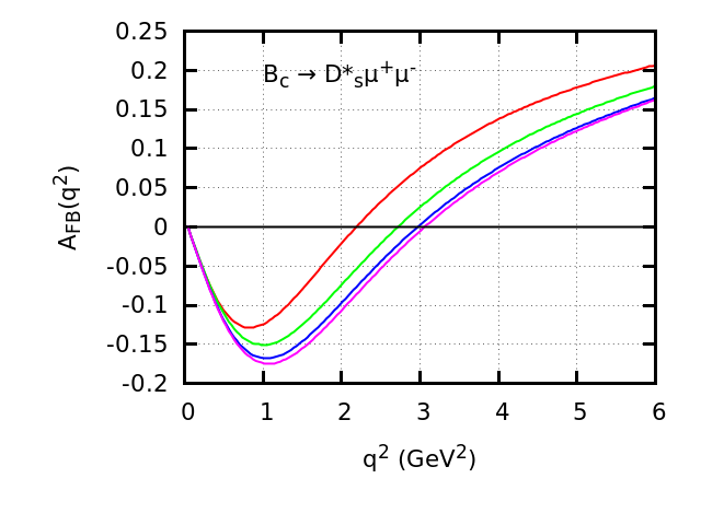
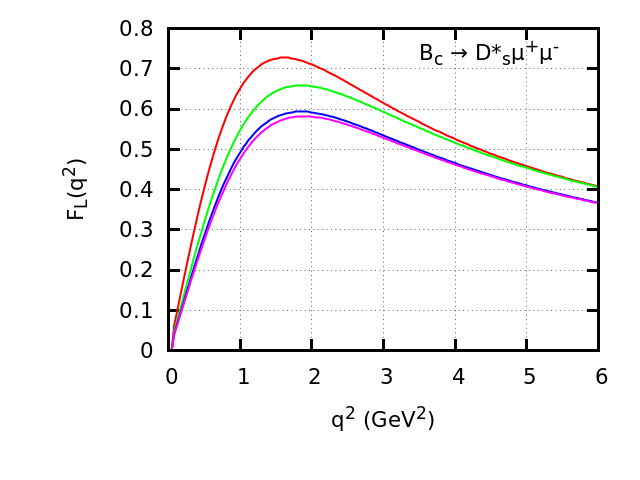
Figure 3: Differential branching ratio $d\mathcal{B}/dq^{2}$, forward backward asymmetry of lepton pair $A_{FB}(q^{2})$ and longitudinal polarization fraction of $D^{\ast}_{s}$ meson $F_{L}(q^{2})$ for the $B_{c}\to D_{s}\mu^{+}\mu^{-}$ and $B_{c}\to D^{\ast}_{s}\mu^{+}\mu^{-}$ decays in the SM (Red) and for the best fit values of new VA couplings in $2D$ scenario. Green, blue and purple lines correspond to the best fit values of $(C_{9}^{NP},\,C_{10}^{NP})=(-0.94,\,+0.23)$, $(C_{9}^{NP},\,C^{\prime}_{9})=(-1.27,\,+0.68)$ and $(C_{9}^{NP},\,C^{\prime}_{10})=(-1.36,\,-0.46)$, respectively.

• The differential branching ratio for the $B_{c}\to D_{s}\mu^{+}\mu^{-}$ decay is reduced at all $q^{2}$ for each NP couplings. The deviation from the SM prediction is more pronounced in case of $(C_{9}^{NP},\,C_{10}^{NP})=(-0.94,\,+0.23)$.

• Similar to $B_{c}\to D_{s}\mu^{+}\mu^{-}$, the differential branching ratio for the $B_{c}\to D^{\ast}_{s}\mu^{+}\mu^{-}$ decay also is reduced at all $q^{2}$. The deviation with the SM prediction, however, increases with increase in $q^{2}$. It reaches maximum at $q^{2}=6\,{\rm GeV^{2}}$.

• The zero crossing in the forward backward asymmetry observable $A_{FB}(q^{2})$ is shifted to higher values of $q^{2}$ than in the SM for each NP couplings. The maximum deviation from the SM prediction is observed for $(C_{9}^{NP},\,C^{\prime}_{10})=(-1.36,\,-0.46)$ which is shown with a purple line in Fig. 3.

• The longitudinal polarization fraction of the $D^{\ast}_{s}$ meson $F_{L}(q^{2})$ decreases once we include the NP couplings. It is observed that the peak of the $F_{L}(q^{2})$ distribution reduces and shifted towards slightly higher $q^{2}$ than in the SM. Maximum deviation from the SM prediction is observed for $(C_{9}^{NP},\,C^{\prime}_{10})=(-1.36,\,-0.46)$ which is shown with a purple line in Fig. 3.

V conclusion

Motivated by the anomalies present in $B\to(K,\,K^{\ast})\mu^{+}\mu^{-}$ decays, we have analyzed $B_{c}\to(D_{s},\,D^{\ast}_{s})\mu^{+}\mu^{-}$ decays mediated via $b\to s\,l^{+}\,l^{-}$ neutral current transitions using the $B_{c}\to(D_{s},\,D^{\ast}_{s})$ transition form factors obtained in the relativistic quark model. We use a model independent effective theory formalism and include NP effects coming from new vector and axial vector operators only. We discard scalar, pseudoscalar and tensor operators as they are severely constrained by $B_{s}\to\mu\mu$ and $b\to s\gamma$ data. Several authors have performed global fits to the $b\to s\,l^{+}\,l^{-}$ data and proposed two types of NP scenarios, namely, $1D$ and $2D$ scenarios. In the $1D$ scenario, we chose four NP scenarios in which the NP contribution is coming from only one NP WCs at a time. In the $2D$ scenario, we chose three NP scenarios in which the NP contribution is coming from two NP WCs at a time.

We give predictions on several observables such as branching ratio, ratio of branching ratio, forward backward asymmetry, and the longitudinal polarization fraction of the $D^{\ast}_{s}$ meson in the SM and in several NP cases. We observe that for most of the NP cases, the branching ratio for both the decay modes is reduced at all $q^{2}$. In most cases, the zero of $A_{FB}(q^{2})$ parameter is shifted to the higher value of $q^{2}$ than in the SM. However, with only $C_{10}^{NP}$, the zero crossing is SM like. Similarly, for the longitudinal polarization fraction of the $D^{\ast}_{s}$ meson, the peak of the distribution is reduced at all $q^{2}$ and it is slightly shifted towards higher value of $q^{2}$ than in the SM.

Although there is hint of NP in $b\to s\,l^{+}\,l^{-}$ transition decays, NP is not yet established. Unlike $B\to(K,\,K^{\ast})\mu^{+}\mu^{-}$ decays which are rigorously studied both theoretically and experimentally, the $B_{c}\to(D_{s},\,D^{\ast}_{s})\mu^{+}\mu^{-}$ decays mediated via same $b\to s\,l^{+}\,l^{-}$ neutral current transitions received very less attention. Measurement of various observables for the $B_{c}\to(D_{s},\,D^{\ast}_{s})\mu^{+}\mu^{-}$ decays and at the same time improved estimates of various $B_{c}\to D_{s}$ and $B_{c}\to D^{\ast}_{s}$ transition form factors in future will be crucial in identifying the true nature of NP. Again, to enhance the significance of various measurements related to $b\to s\,l^{+}\,l^{-}$ decays and to disentangle genuine NP effects from various statistical and systematic uncertainties, more data samples are needed.

*

Appendix A

Here we report the $q^{2}$ bin averaged values of all the observables for the $B_{c}\to(D_{s},\,D^{\ast}_{s})\mu^{+}\mu^{-}$ decays in the SM and in several NP cases.

$q^{2}$ bin (${\rm GeV^{2}})$	SM	$C_{9}^{NP}$	$C_{10}^{NP}$	$C_{9}^{NP}=-C_{10}^{NP}$	$C_{9}^{NP}=-C^{\prime}_{9}$	$(C_{9}^{NP},\,C_{10}^{NP})$	$(C_{9}^{NP},\,C^{\prime}_{9})$	$(C_{9}^{NP},\,C^{\prime}_{10})$
$[0.045,1.0]$	$0.025$	$0.020$	$0.021$	$0.020$	$0.025$	$0.019$	$0.022$	$0.022$
$[1.0,2.0]$	$0.030$	$0.024$	$0.025$	$0.023$	$0.030$	$0.023$	$0.026$	$0.026$
$[2.0,3.0]$	$0.034$	$0.027$	$0.028$	$0.026$	$0.034$	$0.026$	$0.030$	$0.029$
$[3.0,4.0]$	$0.038$	$0.030$	$0.032$	$0.030$	$0.038$	$0.029$	$0.033$	$0.033$
$[4.0,5.0]$	$0.043$	$0.034$	$0.036$	$0.034$	$0.043$	$0.033$	$0.038$	$0.037$
$[5.0,6.0]$	$0.049$	$0.039$	$0.042$	$0.039$	$0.049$	$0.038$	$0.043$	$0.042$
$[1.0,6.0]$	$0.193$	$0.154$	$0.163$	$0.152$	$0.193$	$0.149$	$0.171$	$0.166$

Table 5: $q^{2}$ bin averaged values of $10^{7}\times\mathcal{B}(B_{c}\to D_{s}\mu^{+}\mu^{-})$ in the SM and in several NP cases from $1D$ and $2D$ scenarios.

$q^{2}$ bin (${\rm GeV^{2}})$	SM	$C_{9}^{NP}$	$C_{10}^{NP}$	$C_{9}^{NP}=-C_{10}^{NP}$	$C_{9}^{NP}=-C^{\prime}_{9}$	$(C_{9}^{NP},\,C_{10}^{NP})$	$(C_{9}^{NP},\,C^{\prime}_{9})$	$(C_{9}^{NP},\,C^{\prime}_{10})$
$[0.045,1.0]$	$1.006$	$0.798$	$0.846$	$0.788$	$1.006$	$0.770$	$0.884$	$0.859$
$[1.0,2.0]$	$1.007$	$0.803$	$0.845$	$0.790$	$1.007$	$0.774$	$0.888$	$0.867$
$[2.0,3.0]$	$1.005$	$0.802$	$0.844$	$0.788$	$1.005$	$0.773$	$0.886$	$0.865$
$[3.0,4.0]$	$1.004$	$0.801$	$0.844$	$0.788$	$1.004$	$0.772$	$0.885$	$0.863$
$[4.0,5.0]$	$1.003$	$0.800$	$0.845$	$0.789$	$1.003$	$0.772$	$0.884$	$0.861$
$[5.0,6.0]$	$1.003$	$0.799$	$0.847$	$0.790$	$1.003$	$0.772$	$0.884$	$0.859$
$[1.0,6.0]$	$1.004$	$0.801$	$0.845$	$0.789$	$1.004$	$0.773$	$0.885$	$0.863$

Table 6: $q^{2}$ bin averaged values of $R_{D_{s}}$ in the SM and in several NP cases from $1D$ and $2D$ scenarios.

$q^{2}$ bin (${\rm GeV^{2}})$	SM	$C_{9}^{NP}$	$C_{10}^{NP}$	$C_{9}^{NP}=-C_{10}^{NP}$	$C_{9}^{NP}=-C^{\prime}_{9}$	$(C_{9}^{NP},\,C_{10}^{NP})$	$(C_{9}^{NP},\,C^{\prime}_{9})$	$(C_{9}^{NP},\,C^{\prime}_{10})$
$[0.045,1.0]$	$0.024$	$0.024$	$0.023$	$0.023$	$0.023$	$0.023$	$0.023$	$0.023$
$[1.0,2.0]$	$0.011$	$0.010$	$0.009$	$0.009$	$0.009$	$0.010$	$0.010$	$0.009$
$[2.0,3.0]$	$0.014$	$0.012$	$0.011$	$0.011$	$0.011$	$0.012$	$0.011$	$0.011$
$[3.0,4.0]$	$0.020$	$0.017$	$0.016$	$0.015$	$0.016$	$0.016$	$0.016$	$0.015$
$[4.0,5.0]$	$0.028$	$0.023$	$0.022$	$0.022$	$0.022$	$0.022$	$0.022$	$0.021$
$[5.0,6.0]$	$0.039$	$0.032$	$0.031$	$0.030$	$0.030$	$0.030$	$0.030$	$0.028$
$[1.0,6.0]$	$0.113$	$0.095$	$0.090$	$0.087$	$0.088$	$0.089$	$0.088$	$0.085$

Table 7: $q^{2}$ bin averaged values of $10^{7}\times\mathcal{B}(B_{c}\to D^{\ast}_{s}\mu^{+}\mu^{-})$ in the SM and in several NP cases from $1D$ and $2D$ scenarios.

$q^{2}$ bin (${\rm GeV^{2}})$	SM	$C_{9}^{NP}$	$C_{10}^{NP}$	$C_{9}^{NP}=-C_{10}^{NP}$	$C_{9}^{NP}=-C^{\prime}_{9}$	$(C_{9}^{NP},\,C_{10}^{NP})$	$(C_{9}^{NP},\,C^{\prime}_{9})$	$(C_{9}^{NP},\,C^{\prime}_{10})$
$[0.045,1.0]$	$0.999$	$0.995$	$0.994$	$0.957$	$0.961$	$0.977$	$0.975$	$0.970$
$[1.0,2.0]$	$0.993$	$0.915$	$0.801$	$0.815$	$0.834$	$0.860$	$0.855$	$0.830$
$[2.0,3.0]$	$0.992$	$0.859$	$0.776$	$0.770$	$0.790$	$0.804$	$0.797$	$0.767$
$[3.0,4.0]$	$0.993$	$0.834$	$0.781$	$0.760$	$0.778$	$0.783$	$0.774$	$0.744$
$[4.0,5.0]$	$0.994$	$0.820$	$0.790$	$0.760$	$0.772$	$0.774$	$0.763$	$0.733$
$[5.0,6.0]$	$0.995$	$0.812$	$0.799$	$0.763$	$0.768$	$0.769$	$0.756$	$0.726$
$[1.0,6.0]$	$0.994$	$0.834$	$0.791$	$0.768$	$0.786$	$0.786$	$0.776$	$0.746$

Table 8: $q^{2}$ bin averaged values of $R_{D^{\ast}_{s}}$ in the SM and in several NP cases from $1D$ and $2D$ scenarios.

$q^{2}$ bin (${\rm GeV^{2}})$	SM	$C_{9}^{NP}$	$C_{10}^{NP}$	$C_{9}^{NP}=-C_{10}^{NP}$	$C_{9}^{NP}=-C^{\prime}_{9}$	$(C_{9}^{NP},\,C_{10}^{NP})$	$(C_{9}^{NP},\,C^{\prime}_{9})$	$(C_{9}^{NP},\,C^{\prime}_{10})$
$[0.045,1.0]$	$-0.064$	$-0.069$	$-0.056$	$-0.062$	$-0.072$	$-0.066$	$-0.072$	$-0.072$
$[1.0,2.0]$	$-0.076$	$-0.124$	$-0.079$	$-0.103$	$-0.138$	$-0.121$	$-0.141$	$-0.150$
$[2.0,3.0]$	$0.033$	$-0.028$	$0.035$	$0.006$	$-0.033$	$-0.020$	$-0.043$	$-0.052$
$[3.0,4.0]$	$0.110$	$0.055$	$0.117$	$0.092$	$0.055$	$0.065$	$0.043$	$0.037$
$[4.0,5.0]$	$0.160$	$0.112$	$0.168$	$0.148$	$0.116$	$0.123$	$0.104$	$0.099$
$[5.0,6.0]$	$0.194$	$0.153$	$0.201$	$0.186$	$0.159$	$0.164$	$0.147$	$0.144$
$[1.0,6.0]$	$0.123$	$0.072$	$0.129$	$0.107$	$0.074$	$0.082$	$0.062$	$0.056$

Table 9: $q^{2}$ bin averaged values of $<A_{FB}^{D^{\ast}_{s}}>$ in the SM and in several NP cases from $1D$ and $2D$ scenarios.

$q^{2}$ bin (${\rm GeV^{2}})$	SM	$C_{9}^{NP}$	$C_{10}^{NP}$	$C_{9}^{NP}=-C_{10}^{NP}$	$C_{9}^{NP}=-C^{\prime}_{9}$	$(C_{9}^{NP},\,C_{10}^{NP})$	$(C_{9}^{NP},\,C^{\prime}_{9})$	$(C_{9}^{NP},\,C^{\prime}_{10})$
$[0.045,1.0]$	$0.266$	$0.213$	$0.232$	$0.215$	$0.181$	$0.208$	$0.186$	$0.177$
$[1.0,2.0]$	$0.711$	$0.620$	$0.725$	$0.671$	$0.558$	$0.630$	$0.567$	$0.554$
$[2.0,3.0]$	$0.662$	$0.613$	$0.697$	$0.661$	$0.548$	$0.627$	$0.566$	$0.558$
$[3.0,4.0]$	$0.566$	$0.541$	$0.594$	$0.573$	$0.476$	$0.552$	$0.498$	$0.493$
$[4.0,5.0]$	$0.488$	$0.475$	$0.508$	$0.496$	$0.413$	$0.482$	$0.435$	$0.432$
$[5.0,6.0]$	$0.430$	$0.423$	$0.444$	$0.437$	$0.365$	$0.428$	$0.387$	$0.385$
$[1.0,6.0]$	$0.526$	$0.503$	$0.546$	$0.529$	$0.440$	$0.511$	$0.461$	$0.457$

Table 10: $q^{2}$ bin averaged values of $<F_{L}^{D^{\ast}_{s}}>$ in the SM and in several NP cases from $1D$ and $2D$ scenarios.

References

• (1) R. Aaij et al. [LHCb Collaboration], “Test of lepton universality using $B^{+}\rightarrow K^{+}\ell^{+}\ell^{-}$ decays,” Phys. Rev. Lett.  113, 151601 (2014) doi:10.1103/PhysRevLett.113.151601 [arXiv:1406.6482 [hep-ex]].
• (2) G. Hiller and F. Kruger, “More model-independent analysis of $b\to s$ processes,” Phys. Rev. D 69, 074020 (2004) doi:10.1103/PhysRevD.69.074020 [hep-ph/0310219].
• (3) C. Bobeth, G. Hiller and G. Piranishvili, “Angular distributions of $\bar{B}\to\bar{K}\ell^{+}\ell^{-}$ decays,” JHEP 0712, 040 (2007) doi:10.1088/1126-6708/2007/12/040 [arXiv:0709.4174 [hep-ph]].
• (4) M. Bordone, G. Isidori and A. Pattori, “On the Standard Model predictions for $R_{K}$ and $R_{K^{*}}$,” Eur. Phys. J. C 76 (2016) no.8, 440 doi:10.1140/epjc/s10052-016-4274-7 [arXiv:1605.07633 [hep-ph]].
• (5) R. Aaij et al. [LHCb Collaboration], “Search for lepton-universality violation in $B^{+}\to K^{+}\ell^{+}\ell^{-}$ decays,” Phys. Rev. Lett.  122, no. 19, 191801 (2019) doi:10.1103/PhysRevLett.122.191801 [arXiv:1903.09252 [hep-ex]].
• (6) R. Aaij et al. [LHCb Collaboration], “Test of lepton universality with $B^{0}\rightarrow K^{*0}\ell^{+}\ell^{-}$ decays,” JHEP 1708, 055 (2017) doi:10.1007/JHEP08(2017)055 [arXiv:1705.05802 [hep-ex]].
• (7) B. Capdevila, S. Descotes-Genon, J. Matias and J. Virto, “Assessing lepton-flavour non-universality from $B\to K^{*}\ell\ell$ angular analyses,” JHEP 1610, 075 (2016) doi:10.1007/JHEP10(2016)075 [arXiv:1605.03156 [hep-ph]].
• (8) N. Serra, R. Silva Coutinho and D. van Dyk, “Measuring the breaking of lepton flavor universality in $B\to K^{*}\ell^{+}\ell^{-}$,” Phys. Rev. D 95 (2017) no.3, 035029 doi:10.1103/PhysRevD.95.035029 [arXiv:1610.08761 [hep-ph]].
• (9) A. Abdesselam et al. [Belle Collaboration], “Test of lepton flavor universality in ${B\to K^{\ast}\ell^{+}\ell^{-}}$ decays at Belle,” arXiv:1904.02440 [hep-ex]. i
• (10) S. Descotes-Genon, J. Matias, M. Ramon and J. Virto, “Implications from clean observables for the binned analysis of $B->K*\mu^{+}\mu^{-}$ at large recoil,” JHEP 1301, 048 (2013) doi:10.1007/JHEP01(2013)048 [arXiv:1207.2753 [hep-ph]].
• (11) S. Descotes-Genon, T. Hurth, J. Matias and J. Virto, “Optimizing the basis of $B\to K^{*}ll$ observables in the full kinematic range,” JHEP 1305, 137 (2013) doi:10.1007/JHEP05(2013)137 [arXiv:1303.5794 [hep-ph]].
• (12) R. Aaij et al. [LHCb Collaboration], “Measurement of Form-Factor-Independent Observables in the Decay $B^{0}\to K^{*0}\mu^{+}\mu^{-}$,” Phys. Rev. Lett.  111 (2013) 191801 doi:10.1103/PhysRevLett.111.191801 [arXiv:1308.1707 [hep-ex]].
• (13) R. Aaij et al. [LHCb Collaboration], “Angular analysis of the $B^{0}\to K^{*0}\mu^{+}\mu^{-}$ decay using 3 fb-1 of integrated luminosity,” JHEP 1602, 104 (2016) doi:10.1007/JHEP02(2016)104 [arXiv:1512.04442 [hep-ex]].
• (14) M. Aaboud et al. [ATLAS Collaboration], “Angular analysis of $B^{0}_{d}\rightarrow K^{*}\mu^{+}\mu^{-}$ decays in $pp$ collisions at $\sqrt{s}=8$ TeV with the ATLAS detector,” JHEP 1810, 047 (2018) doi:10.1007/JHEP10(2018)047 [arXiv:1805.04000 [hep-ex]].
• (15) J. Aebischer, J. Kumar, P. Stangl and D. M. Straub, “A Global Likelihood for Precision Constraints and Flavour Anomalies,” arXiv:1810.07698 [hep-ph].
• (16) A. Abdesselam et al. [Belle Collaboration], “Angular analysis of $B^{0}\to K^{\ast}(892)^{0}\ell^{+}\ell^{-}$,” arXiv:1604.04042 [hep-ex].
• (17) CMS Collaboration [CMS Collaboration], ”Measurement of the $P_{1}$ and $P^{\prime}_{5}$ angular parameters of the decay $B^{0}\to K^{{\ast}^{0}}\mu^{+}\mu^{-}$ in proton-proton collisions at $\sqrt{s}=8\,{\rm TeV}$,” CMS-PAS-BPH-15-008.
• (18) R. Aaij et al. [LHCb Collaboration], “Differential branching fraction and angular analysis of the decay $B_{s}^{0}\to\phi\mu^{+}\mu^{-}$,” JHEP 1307, 084 (2013) doi:10.1007/JHEP07(2013)084 [arXiv:1305.2168 [hep-ex]].
• (19) R. Aaij et al. [LHCb Collaboration], “Angular analysis and differential branching fraction of the decay $B^{0}_{s}\to\phi\mu^{+}\mu^{-}$,” JHEP 1509, 179 (2015) doi:10.1007/JHEP09(2015)179 [arXiv:1506.08777 [hep-ex]].
• (20) A. Bharucha, D. M. Straub and R. Zwicky, “$B\to V\ell^{+}\ell^{-}$ in the Standard Model from light-cone sum rules,” JHEP 1608, 098 (2016) doi:10.1007/JHEP08(2016)098 [arXiv:1503.05534 [hep-ph]].
• (21) B. Capdevila, A. Crivellin, S. Descotes-Genon, J. Matias and J. Virto, “Patterns of New Physics in $b\to s\ell^{+}\ell^{-}$ transitions in the light of recent data,” JHEP 1801, 093 (2018) doi:10.1007/JHEP01(2018)093 [arXiv:1704.05340 [hep-ph]].
• (22) W. Altmannshofer, P. Stangl and D. M. Straub, “Interpreting Hints for Lepton Flavor Universality Violation,” Phys. Rev. D 96, no. 5, 055008 (2017) doi:10.1103/PhysRevD.96.055008 [arXiv:1704.05435 [hep-ph]].
• (23) G. D’Amico, M. Nardecchia, P. Panci, F. Sannino, A. Strumia, R. Torre and A. Urbano, “Flavour anomalies after the $R_{K^{*}}$ measurement,” JHEP 1709, 010 (2017) doi:10.1007/JHEP09(2017)010 [arXiv:1704.05438 [hep-ph]].
• (24) G. Hiller and I. Nisandzic, “$R_{K}$ and $R_{K^{\ast}}$ beyond the standard model,” Phys. Rev. D 96, no. 3, 035003 (2017) doi:10.1103/PhysRevD.96.035003 [arXiv:1704.05444 [hep-ph]].
• (25) L. S. Geng, B. Grinstein, S. Jäger, J. Martin Camalich, X. L. Ren and R. X. Shi, “Towards the discovery of new physics with lepton-universality ratios of $b\to s\ell\ell$ decays,” Phys. Rev. D 96, no. 9, 093006 (2017) doi:10.1103/PhysRevD.96.093006 [arXiv:1704.05446 [hep-ph]].
• (26) M. Ciuchini, A. M. Coutinho, M. Fedele, E. Franco, A. Paul, L. Silvestrini and M. Valli, “On Flavourful Easter eggs for New Physics hunger and Lepton Flavour Universality violation,” Eur. Phys. J. C 77, no. 10, 688 (2017) doi:10.1140/epjc/s10052-017-5270-2 [arXiv:1704.05447 [hep-ph]].
• (27) A. Celis, J. Fuentes-Martin, A. Vicente and J. Virto, “Gauge-invariant implications of the LHCb measurements on lepton-flavor nonuniversality,” Phys. Rev. D 96, no. 3, 035026 (2017) doi:10.1103/PhysRevD.96.035026 [arXiv:1704.05672 [hep-ph]].
• (28) A. K. Alok, B. Bhattacharya, A. Datta, D. Kumar, J. Kumar and D. London, “New Physics in $b\to s\mu^{+}\mu^{-}$ after the Measurement of $R_{K^{*}}$,” Phys. Rev. D 96, no. 9, 095009 (2017) doi:10.1103/PhysRevD.96.095009 [arXiv:1704.07397 [hep-ph]].
• (29) A. K. Alok, B. Bhattacharya, D. Kumar, J. Kumar, D. London and S. U. Sankar, “New physics in $b\rightarrow s\mu^{+}\mu^{-}$: Distinguishing models through CP-violating effects,” Phys. Rev. D 96, no. 1, 015034 (2017) doi:10.1103/PhysRevD.96.015034 [arXiv:1703.09247 [hep-ph]].
• (30) A. K. Alok, A. Dighe, S. Gangal and D. Kumar, “Continuing search for new physics in $b\to s\mu\mu$ decays: two operators at a time,” arXiv:1903.09617 [hep-ph].
• (31) A. Faessler, T. Gutsche, M. A. Ivanov, J. G. Korner and V. E. Lyubovitskij, “The Exclusive rare decays $B\to$ K(K*) $\bar{\ell}\ell$ and $B_{c}\to$ D(D*) $\bar{\ell}\ell$ in a relativistic quark model,” Eur. Phys. J. direct 4, no. 1, 18 (2002) doi:10.1007/s1010502c0018 [hep-ph/0205287].
• (32) C. Q. Geng, C. W. Hwang and C. C. Liu, “Study of rare $B^{+}_{c}\to D_{d,s}$ + lepton anti-lepton decays,” Phys. Rev. D 65, 094037 (2002) doi:10.1103/PhysRevD.65.094037 [hep-ph/0110376].
• (33) H. M. Choi, “Light-front quark model analysis of the exclusive rare $B_{c}\to D_{(s)}(\ell^{+}\ell^{-},\nu_{\ell}\bar{\nu}_{\ell})$ decays,” Phys. Rev. D 81, 054003 (2010) doi:10.1103/PhysRevD.81.054003 [arXiv:1001.3432 [hep-ph]].
• (34) K. Azizi, F. Falahati, V. Bashiry and S. M. Zebarjad, “Analysis of the Rare B(c) —¿ D*(s,d) l+ l- Decays in QCD,” Phys. Rev. D 77, 114024 (2008) doi:10.1103/PhysRevD.77.114024 [arXiv:0806.0583 [hep-ph]].
• (35) K. Azizi and R. Khosravi, “Analysis of the rare semileptonic $B_{c}\to P(D,D_{s})\ell^{+}\ell^{-}/\nu\bar{\nu}$ decays within QCD sum rules,” Phys. Rev. D 78, 036005 (2008) doi:10.1103/PhysRevD.78.036005 [arXiv:0806.0590 [hep-ph]].
• (36) D. Ebert, R. N. Faustov and V. O. Galkin, “Rare Semileptonic Decays of $B$ and $B_{c}$ Mesons in the Relativistic Quark Model,” Phys. Rev. D 82, 034032 (2010) doi:10.1103/PhysRevD.82.034032 [arXiv:1006.4231 [hep-ph]].
• (37) A. K. Alok, A. Datta, A. Dighe, M. Duraisamy, D. Ghosh and D. London, JHEP 1111, 121 (2011) doi:10.1007/JHEP11(2011)121 [arXiv:1008.2367 [hep-ph]].
• (38) A. K. Alok, A. Datta, A. Dighe, M. Duraisamy, D. Ghosh and D. London, JHEP 1111, 122 (2011) doi:10.1007/JHEP11(2011)122 [arXiv:1103.5344 [hep-ph]].
• (39) D. Bardhan, P. Byakti and D. Ghosh, Phys. Lett. B 773, 505 (2017) doi:10.1016/j.physletb.2017.08.062 [arXiv:1705.09305 [hep-ph]].
• (40) M. Beneke, T. Feldmann and D. Seidel, “Systematic approach to exclusive $B\to Vl^{+}l^{-}$, $V\gamma$ decays,” Nucl. Phys. B 612, 25 (2001) doi:10.1016/S0550-3213(01)00366-2 [hep-ph/0106067].
• (41) M. Beneke, T. Feldmann and D. Seidel, “Exclusive radiative and electroweak $b\to d$ and $b\to s$ penguin decays at NLO,” Eur. Phys. J. C 41, 173 (2005) doi:10.1140/epjc/s2005-02181-5 [hep-ph/0412400].
• (42) A. J. Buras and M. Munz, “Effective Hamiltonian for B —¿ X(s) e+ e- beyond leading logarithms in the NDR and HV schemes,” Phys. Rev. D 52, 186 (1995) doi:10.1103/PhysRevD.52.186 [hep-ph/9501281].
• (43) J. Charles, A. Le Yaouanc, L. Oliver, O. Pene and J. C. Raynal, “Heavy to light form-factors in the heavy mass to large energy limit of QCD,” Phys. Rev. D 60, 014001 (1999) doi:10.1103/PhysRevD.60.014001 [hep-ph/9812358].
• (44) D. Ebert, R. N. Faustov and V. O. Galkin, “Form-factors of heavy to light B decays at large recoil,” Phys. Rev. D 64, 094022 (2001) doi:10.1103/PhysRevD.64.094022 [hep-ph/0107065].
• (45) J. G. Korner and G. A. Schuler, “Exclusive Semileptonic Heavy Meson Decays Including Lepton Mass Effects,” Z. Phys. C 46, 93 (1990).
• (46) A. Kadeer, J. G. Korner and U. Moosbrugger, “Helicity analysis of semileptonic hyperon decays including lepton mass effects,” Eur. Phys. J. C 59, 27 (2009) [hep-ph/0511019].
• (47) M. Tanabashi et al. [Particle Data Group], “Review of Particle Physics,” Phys. Rev. D 98, no. 3, 030001 (2018). doi:10.1103/PhysRevD.98.030001
• (48) W. Altmannshofer, P. Ball, A. Bharucha, A. J. Buras, D. M. Straub and M. Wick, JHEP 0901, 019 (2009) doi:10.1088/1126-6708/2009/01/019 [arXiv:0811.1214 [hep-ph]].
• (49) M. Bona et al. [UTfit Collaboration], “The Unitarity Triangle Fit in the Standard Model and Hadronic Parameters from Lattice QCD: A Reappraisal after the Measurements of Delta m(s) and BR(B —¿ tau nu(tau)),” JHEP 0610, 081 (2006) doi:10.1088/1126-6708/2006/10/081 [hep-ph/0606167].
• (50) A. Ali, P. Ball, L. T. Handoko and G. Hiller, “A Comparative study of the decays $B\to$ ($K$, $K^{*)}\ell^{+}\ell^{-}$ in standard model and supersymmetric theories,” Phys. Rev. D 61, 074024 (2000) doi:10.1103/PhysRevD.61.074024 [hep-ph/9910221].