Strongly Interacting Neutrino Portal Dark Matter

Abstract

We present a realistic, simple and natural model of strongly-interacting dark matter based on the neutrino-portal paradigm. The strong interactions at small velocities are generated by the exchange of dark photons, and produce the observed core-like DM distribution in galactic centers; this effect could be spoiled by the formation of DM bound states (also due to dark-photon effects), which we avoid by requiring the DM candidates to be light, with masses below $O(10\,\hbox{GeV})$. The mixing of the dark photon with the $Z$ and ordinary photon is strongly suppressed by introducing a softly-broken discrete symmetry similar to charge conjugation, which also ensures that the dark photon life-time is short enough to avoid restrictions derived form big-bang nucleosynthesis and large-scale structure formation. Other constraints are accommodated without the need of fine tuning, in particular nucleon scattering occurs only at one loop, so direct detection cross sections are naturally suppressed. Neutrino masses are generated through the inverse see saw.

1 Introduction

The nature of dark matter (DM) remains one of the most perplexing problems in modern particle and astroparticle physics. Current evidence for the existence of massive particles that interact weakly with the Standard Model (SM) is entirely gravitational Zwicky:1933gu ; Rubin:1970zza ; Corbelli:1999af ; Allen:2011zs ; Clowe:2006eq , and every attempt at direct Hanany:2019lle ; Behnke:2016lsk ; Fu:2016ega ; Akerib:2016lao ; Aprile:2017iyp ; Akerib:2016vxi ; Tan:2016zwf , indirect Bulbul:2014sua ; Ruchayskiy:2015onc ; Franse:2016dln ; Urban:2014yda ; Aharonian:2016gzq ; Choi:2015ara ; Aartsen:2016zhm ; TheFermi-LAT:2017vmf ; Hooper:2010mq ; Ackermann:2015zua ; Cui:2016ppb or collider Aaboud:2016wna ; Sirunyan:2018gka ; Abercrombie:2015wmb detection has only led to increasingly stronger constraints on models. In addition, estimations of the DM distribution in dwarf galaxies indicate that the DM density at the core does not exhibit a spike, as would be expected if it behaved as an ideal gas. This “core vs. cusp” problem deBlok:2009sp ; Flores:1994gz ; Moore:1994yx ; Moore:1999gc can be alleviated Spergel:1999mh ; Tulin:2017ara by including self-interactions within the dark sector; such interactions must be relatively strong and velocity-dependent. Models of this type are often referred to as strongly-interacting dark matter (SIDM) models.

In this paper we will discuss a simple SIDM model that meets all available constraints without fine tuning of parameters. The model is an extension of one discussed earlier Gonzalez-Macias:2016vxy ; Gonzalez-Macias:2016snw , based on the neutrino-portal paradigm Cosme:2005sb ; Falkowski:2009yz ; An:2009vq ; Lindner:2010rr ; Falkowski:2011xh ; Farzan:2011ck ; Heeck:2012bz ; Baek:2013qwa ; Baldes:2015lka ; Gonzalez-Macias:2016vxy ; Gonzalez-Macias:2016snw ; Batell:2017rol ; HajiSadeghi:2017zrl ; Berlin:2018ztp ; Bandyopadhyay:2018qcv ; Blennow:2019fhy where the dark sector couples to the SM via (Dirac) fermion mediators that mix with the SM neutrinos. The dark sector contains two quasi-degenerate fermions, which constitute the relic density, and a scalar, more massive than the fermions. Interactions within the dark sector are mediated by a dark photon, whose mixing with the ordinary photon is (again, naturally) strongly suppressed, since it occurs at three loops; the main decay mode of the dark photon is into neutrinos, and appears at one loop, so the dark photon is relatively long-lived. Of special interest is that the DM self-interactions are useful in suppressing a possible cusp in the DM galactic distribution only when the DM mass is light, below $O(10)$ GeV.

The paper is organized as follows: in the next section we describe our model Gonzalez-Macias:2016vxy concentrating on the interactions within the dark sector; detailed discussion of the other aspects can be found in the original paper. In sections 3, 4 and 5 we discuss the electroweak, relic abundance and direct-detection constraints respectively. Section 6 contains results from numerical simulations, and we present our conclusions in section 7.

2 The Model

As noted above, we will study an extension of the neutrino portal dark matter model discussed in Gonzalez-Macias:2016vxy , where we add self-interactions to the dark sector, and double the number of fermions (the justification for this is provided below). The dark sector then contains two fermions $\Psi_{\pm}$ with masses $m_{\pm}$, and one complex scalar $\Phi$ with mass $m_{\Phi}>m_{\pm}$; the fermions correspond to the DM. The dark sector is connected to the Standard Model through a set of three (Dirac) neutral fermionic mediators ${\cal F}$ with interactions of the form $\bar{\Psi}\Phi{\cal F}$ and  $\bar{l}{\cal F}\tilde{\phi}$.

We generate interactions within the dark sector by assuming the dark sector has a $U(1)_{\tt dark}$ gauge symmetry under which $\Psi_{\pm}$ and $\Phi$ are charged; we denote by $V$ the corresponding gauge boson, the dark photon. To implement the SIDM paradigm we will assume the $V$ has a non-zero mass $m_{\tt V}$ that we introduce using the Stückelberg trick. The cross sections generated by $V$ exchange can then generate self-interactions with the velocity dependence Tulin:2017ara required to address the core vs. cusp problem.

Models of this type contain a kinetic mixing term of the form $\xi V_{\mu\nu}B^{\mu\nu}$ Holdom:1985ag , where $B$ is the Standard Model hypercharge gauge field. The coupling $\xi$ is strongly constrained by data: $\xi\leq 10^{-3}$ Alexander:2016aln ; we interpret this as an indication that the model should contain a symmetry that forbids this interaction and which is either exact or softly broken. For this reason we impose a dark $\mathbb{Z}_{2}$ symmetry (dark charge conjugation – DCC) under which $V$ is odd and all SM particles are even: the dark scalar has the expected $\Phi\rightarrow\Phi^{*}$ behavior, while $\{\Psi_{+},\,\Psi_{-}\}$, form a dark-charge doublet, exchanged under DCC:

$$\mbox{DCC:}\quad\Psi_{+}\leftrightarrow\Psi_{-}\,,\quad\Phi\leftrightarrow\Phi^{*}\,,\quad V\leftrightarrow-V\,.$$ (1)

The DCC symmetry requires that $\Psi_{+}$ and $\Psi_{-}$ have the same mass and couplings; and it also implies that a sufficiently light $V$ will be stable, which is phenomenologically troublesome. For this last reason we will assume that DCC is softly broken by assuming the $\Psi_{\pm}$ masses are split (this is the only way to achieve this soft braking with the particle content we assume).

The Lagrangian for this model is then given by

$${\cal L}= \bar{\Psi}_{+}(i\not{D}_{+}-m_{+})\Psi_{+}+\bar{\Psi}_{-}(i\not{D}_{-}-m_{-})\Psi_{-}+|D\Phi|^{2}$$

$$-\frac{1}{2}m_{\Phi}^{2}|\Phi|^{2}-\frac{1}{4}\lambda|\Phi|^{4}-\frac{1}{4}V_{\mu\nu}V^{\mu\nu}+\frac{1}{2}m_{\tt V}^{2}\left(V_{\mu}-\frac{1}{m_{\tt V}}\partial_{\mu}\sigma\right)^{2}+\bar{{\cal F}}(i\not{\partial}-m_{\cal F}){\cal F}$$

$$-\left[\bar{l}Y^{(\nu)}{\cal F}\tilde{\phi}+\mbox{H.c.}\right]-\left[\left(\bar{\Psi}_{+}\Phi+\bar{\Psi}_{-}\Phi^{*}\right)(z{\cal F})+\mbox{H.c.}\right]-\lambda_{x}|\Phi|^{2}|\phi|^{2}\,,$$ (2)

where, as noted above, $l$ is the SM left-handed lepton isodoublet and $\phi$ the SM isodoublet; also

$$D^{\alpha}_{\pm}=\partial^{\alpha}\pm igV^{\alpha}$$ (3)

is the covariant derivative, and

$$m_{\pm}=m_{\Psi}\pm\mu\,,$$ (4)

where $\mu$, the fermion mass splitting, parameterizes the soft breaking of DCC; $\sigma$ is the auxiliary field used in the Stückelberg trick (the unitary gauge corresponds to $\sigma=0$). Finally, we assume three ${\cal F}$ fields , hence $m_{\cal F}$ and $Y^{\left(\nu\right)}$ are $3\times 3$ mass and Yukawa coupling matrices, respectively, and $z$ is a $3\times 1$ vector.

Compared to the earlier version, this model has 3 additional parameters: $\mu,\,g$ and $m_{\tt V}$. We will see (cf. Sect. 2.2), however, that the constraints on the DM self-interactions are sufficient to fix $m_{\tt V}$ and $g$ as functions of $m_{\Psi}$, so that, in fact only one additional free parameter is introduced.

Once the Standard Model symmetry is broken the neutrinos $\nu_{L}$ (contained in $l$) will mix with the ${\cal F}$; we will denote the mass eigenstates as $n_{L}$, left-handed and massless, and $N$, with a mass of order $m_{\cal F}$. To reduce the number of parameters we will assume for simplicity that the $N$ are degenerate, with mass $m_{\tt N}$. In this case the gauge and mass eigenstates are related by

$${\cal F} ={\cal C}N_{L}+{\cal S}n_{L}+N_{R}\,;$$

$$\nu =V_{\tt PMNS}^{\dagger}\left({\cal C}n_{L}-{\cal S}N_{L}\right)\,,$$ (5)

where $V_{\tt PMNS}$ is the usual PMNS matrix, and ${\cal S}$ and ${\cal C}$ are diagonal $3\times 3$ mixing matrices that obey

$${\cal S}^{2}+{\cal C}^{2}={\mathbbm{1}}\,.$$ (6)

In terms of these quantities

$$m_{\cal F}=m_{\tt N}{\cal C}\,,\quad Y^{\left(\nu\right)}=\sqrt{2}\frac{m_{\tt N}}{v_{\tt H}}V_{\tt PMNS}^{\dagger}{\cal S}\,,$$ (7)

where $v_{\tt H}$ denotes the Higgs vacuum expectation value.

As a last simplification we will assume that the $z$ Yukawa couplings are real; in this case the model has 11 parameters: $\{m_{\tt N},\,m_{\Psi},\,m_{\Phi},\,\mu\}(4),~{}\{z,\,{\cal S},\,\lambda_{x}\}(7)$.

The various interaction terms involving the $n_{L}$ and $N$ take the form

$$Z~{}\mbox{couplings:} \quad-\frac{g}{2c_{\tt W}}\left[\bar{n}_{L}{\cal C}^{2}\not{Z}n_{L}+\bar{N}_{L}{\cal S}^{2}\not{Z}N_{L}+\left(\bar{n}_{L}{\cal C}{\cal S}\not{Z}N_{L}+{\rm H.c.}\right)\right]\,.$$

$$W~{}\mbox{couplings:} \quad-\frac{g}{\sqrt{2}}\left[\bar{e}\not{W}V^{\dagger}_{\tt PMNS}{\cal C}n_{L}-\bar{e}\not{W}V^{\dagger}_{\tt PMNS}{\cal S}N_{L}+{\rm H.c.}\right]\,.$$

Yukawa couplings: $$\quad+\frac{m_{\tt N}}{v_{\tt H}}H\left[\bar{N}_{R}{\cal S}{\cal C}n_{L}-\bar{N}_{R}{\cal S}^{2}N_{L}+{\rm H.c}\right]\,.$$

DM couplings: $$\quad+\left[\bar{\Psi}_{\pm}\Phi z{\cal S}n_{L}+\bar{\Psi}_{\pm}\Phi z({\cal C}P_{L}+P_{R})N+{\rm H.c}\right]+\lambda_{x}|\phi|^{2}|\Phi|^{2}\,.$$ (8)

We identify the $n_{L}$ with the observed neutrinos, however, these are massless, as noted above – but this can be easily remedied by introducing a small Majorana mass term for the ${\cal F}$: $\bar{\cal F}M_{\tt Maj}{\cal F}^{c}+\mbox{H.c.}$ The effect is to slightly break the degeneracy of the $N$ and to give a Majorana mass to the $n_{L}$, whose form is the same as the one obtained in the inverse see-saw scheme Wyler:1982dd ; Mohapatra:1986bd ; Ma:1987zm . The $M_{\tt Maj}$ term represent a soft and explicit breaking of lepton number, so the smallness of the neutrino masses is (technically) natural; since this mass matrix is arbitrary, it can be used to generate the observed masses and mixing angles in the neutrino sector.

As a matter of notation we find it convenient to define

$$r_{{\tt i}{\tt j}}=\left(\frac{m_{\tt i}}{m_{\tt j}}\right)^{2}\,,$$ (9)

so that $r_{{\tt N}{\tt Z}}=(m_{\tt N}/m_{\tt Z})^{2}$, etc.

      

Figure 1: Loop graphs generating the $\Psi\Psi Z$ and $\Psi\Psi H$ couplings.

2.1 Loop-induced couplings

The above model has no tree-level couplings of the DM ($\Psi$) to the $Z$ and $H$ bosons. These couplings are generated at 1 loop by the graphs in Fig. 1. Assuming zero external momenta a straightforward calculation gives Gonzalez-Macias:2016vxy

$${\cal L}_{\tt DM-Z} =-\frac{g}{2c_{\tt W}}\bar{\Psi}_{\pm}\not{Z}\left(\epsilon_{L}P_{L}+\epsilon_{R}P_{R}\right)\Psi_{\pm}\,;$$

$${\cal L}_{\tt DM-H} =\epsilon_{H}\bar{\Psi}_{\pm}\Psi_{\pm}H\,,$$ (10)

where (see eq. 9)

$$\epsilon_{R} =-\frac{(z{\cal S}^{2}{\cal C}^{2}z^{T})}{32\pi^{2}}\,\,\frac{1-r_{\Phi{\tt N}}+\ln r_{\Phi{\tt N}}}{(1-r_{\Phi{\tt N}})^{2}}\,;$$

$$\epsilon_{L} =\frac{(z{\cal S}^{2}z^{T})}{16\pi^{2}}\,\frac{1-r_{\Phi{\tt N}}+r_{\Phi{\tt N}}\ln r_{\Phi{\tt N}}}{(1-r_{\Phi{\tt N}})^{2}}\,;$$

$$\epsilon_{H} =-\frac{1}{8\pi^{2}}\frac{m_{\tt N}}{v_{\tt H}}\left\{(z{\cal S}^{2}{\cal C}z^{T})\frac{1-r_{\Phi{\tt N}}+r_{\Phi{\tt N}}\ln r_{\Phi{\tt N}}}{(r_{\Phi{\tt N}}-1)^{2}}+\frac{1}{2}\lambda_{x}\frac{v_{\tt H}^{2}}{m_{\tt N}^{2}}(z{\cal C}z^{T})\frac{1-r_{\Phi{\tt N}}+\ln r_{\Phi{\tt N}}}{(r_{\Phi{\tt N}}-1)^{2}}\right\}\,.$$ (11)

2.2 DM self-interactions:

The strong-interactions of the SIDM paradigm are generated in this model by $\Psi$ scattering mediated by $V$ exchange. There are two such reactions: $\Psi_{\pm}\Psi_{\pm}\rightarrow\Psi_{\pm}\Psi_{\pm}$ and $\Psi_{+}\Psi_{-}\rightarrow\Psi_{+}\Psi_{-}$, with cross section $\sigma_{\tt r}$ and $\sigma_{\tt a}$, respectively (the first is the same as Möller scattering with a massive photon). The calculation is straightforward, using

$$\beta_{\Psi}=\sqrt{1-\frac{4m_{\Psi}^{2}}{s}}\,,$$ (12)

and neglecting the DM mass difference, we find

$$\frac{\sigma_{\tt r}}{m_{\Psi}} =\frac{g^{4}}{4\pi sm_{\Psi}}\Biggl{\{}\frac{(2s+3m_{\tt V}^{2})s\beta_{\Psi}^{2}+2(m_{\tt V}^{2}+2m_{\Psi}^{2})^{2}}{2m_{\tt V}^{2}(m_{\tt V}^{2}+s\beta_{\Psi}^{2})}$$

$$\hskip 72.26999pt-\frac{(s\beta_{\Psi}^{2}+2m_{\tt V}^{2})(3m_{\tt V}^{2}+4m_{\Psi}^{2})+2(m_{\tt V}^{2}+2m_{\Psi}^{2})^{2}-4m_{\Psi}^{4}}{s\beta_{\Psi}^{2}\left(2m_{\tt V}^{2}+s\beta_{\Psi}^{2}\right)}\ln\left(1+\frac{s\beta_{\Psi}^{2}}{m_{\tt V}^{2}}\right)\Biggr{\}}\,;$$

$$\frac{\sigma_{\tt a}}{m_{\Psi}} =\frac{g^{4}}{4\pi sm_{\Psi}}\left\{\frac{(2s+3m_{\tt V}^{2})s\beta_{\Psi}^{2}+2(m_{\tt V}^{2}+2m_{\Psi}^{2})^{2}}{2m_{\tt V}^{2}\left(m_{\tt V}^{2}+s\beta_{\Psi}^{2}\right)}-\frac{\left(m_{\tt V}^{2}+s\right)}{s\beta_{\Psi}^{2}}\ln\left(1+\frac{s\beta_{\Psi}^{2}}{m_{\tt V}^{2}}\right)\right\}\,.$$ (13)

These cross sections are enhanced when $m_{\Psi}\gg m_{\tt V}$ and the relative velocity $\beta_{\Psi}$ is small; in this regime the $V$ interactions generate the required strong interactions.

Since $\Psi_{+}$ and $\Psi_{-}$ have but a small mass difference, and have identical couplings, they will have the same relic abundance density $n$. In this case the effective DM-DM cross section will be $(\sigma_{\tt r}+\sigma_{\tt a})/2$. To see this, note that a $\Psi_{+}$ moving with speed v; in a time $\delta t$ it will have $n\sigma_{++}{\tt v}\delta t$ interactions with other $\Psi_{+}$, and $n\sigma_{+-}{\tt v}\delta t$ interactions with the $\Psi_{-}$; the total number of interactions will be then (using $n=n_{\tt DM}/2$),

$$\frac{n_{\tt DM}}{2}\left(\sigma_{\tt r}+\sigma_{\tt a}\right){\tt v}\delta t=n_{\tt DM}\sigma_{\tt eff}{\tt v}\delta t{\quad\Rightarrow\quad}\sigma_{\tt eff}=\frac{\sigma_{\tt r}+\sigma_{\tt a}}{2}\,.$$ (14)

Note that $\sigma_{\tt eff}$ depends on the relative velocity v.

Existing data constraints the SIDM cross section for galaxy clusters and for dwarf and low-surface-brightness galaxies; since the typical velocity in each environment is different, the cross section must have an appropriate velocity-dependence. The central values of the cross sections and velocities are  Kaplinghat:2015aga

$$\left.\frac{\sigma_{\tt eff}}{m_{\Psi}}\right|_{\rm galaxy}=1.9\frac{\hbox{cm}^{2}}{\hbox{gr}}\,,~{}\left.\frac{\sigma_{\tt eff}}{m_{\Psi}}\right|_{\rm cluster}=0.1\frac{\hbox{cm}^{2}}{\hbox{gr}}\,;\quad\left.\beta_{\Psi}\right|_{\rm galaxy}=3.3\times 10^{-4}\,,~{}\left.\beta_{\Psi}\right|_{\rm cluster}=5.4\times 10^{-3}\,.$$ (15)

Fitting eqs. 13 and 14 we find 

$$m_{\tt V}=\frac{m_{\Psi}}{443}\,,\qquad g=\left(\frac{m_{\Psi}}{64\,\hbox{GeV}}\right)^{3/4}\,.$$ (16)

These expressions have significant errors; using Kaplinghat:2015aga we estimate

$$443\rightarrow(116,\,1557)\,,\qquad 64\,\hbox{GeV}\rightarrow(17,\,225)\,\hbox{GeV}\,.$$ (17)

In our numerical calculations we will be conservative and assume that these are uncertain by up to a factor of 3 (e.g., the first ranges from $443/3$ to $3*443$).

The DCC symmetry, despite being softly broken, is very effective in limiting the number of couplings of the $V$ that can have any phenomenological significance. For example, $V-Z$ and $V-\gamma$ mixings occur only at 2 and 3 loops, respectively, and can be ignored. The only interesting 1-loop vertex is considered in the next section.

2.3 Decay of the $V$

In the absence of the DCC breaking term $\propto\mu$ in eq. 2, the massive dark photon $V$ is stable, which presents something of a problem: once it decouples from the $\Psi$, its abundance would be fixed., and since it is also light [cf. eq. 16] , its presence would make the model inconsistent with big-bang nucleosynthesis (BBN) Ahlgren:2013wba and large scale structure formation (LSS) Zhang:2015era constraints. This is avoided when $\mu\not=0$, that is, when the $\Psi_{\pm}$ mass degeneracy is broken.

Figure 2: Graphs responsible for a non-zero decay width for the $V$.

In this case, the graphs in Fig. 2 give

$$\Gamma(V\rightarrow\bar{n}_{L}n_{L})=\frac{m_{\tt V}}{6\pi}\left\{\frac{g}{16\pi^{2}}\left[f\left(\frac{m_{+}}{m_{\Phi}}\right)-f\left(\frac{m_{-}}{m_{\Phi}}\right)\right]\right\}^{2}\left(z{\cal S}^{2}z^{\dagger}\right)^{2}\,,$$ (18)

where we assumed $m_{\Psi}\gg m_{\tt V},\,\mu$, and defined

$$f(x)=\frac{1}{4}\left(\frac{x^{2}+1}{x^{2}-1}\right)-\left(\frac{x^{2}}{x^{2}-1}\right)^{2}\ln\,x\,.$$ (19)

As before, $m_{\pm}=m_{\Psi}\pm\mu$ denote the mass of $\Psi_{+}$ and $\Psi_{-}$, respectively. The BBN and LSS constraints on this decay width are relatively mild: $1/\Gamma(V\rightarrow\bar{n}_{L}n_{L})<1$s, which we adopt in the numerical calculations.

2.4 Bound States

The inclusion of a strong interaction between DM particles opens up the possibility that the $\Psi_{+}$ and $\Psi_{-}$, having opposite charges, will form bound states. If this were to happen the strong interactions would be screened and the cusp problem would reappear. To avoid this we now consider the conditions for such bound states not to form.

In the non-relativistic limit, the $V$ exchange generates an attractive Yukawa potential between the $\Psi_{+}$ and $\Psi_{-}$:

$$\mathcal{V}_{NR}=\frac{g^{2}}{4\pi}\frac{e^{-m_{\tt V}r}}{r}\,.$$ (20)

If a bound state is formed then its typical size is determined by the range of the potential, $\sim 1/m_{\tt V}$; it follows that the typical kinetic energy of the $\Psi$ will be $\sim m_{\tt V}^{2}/m_{\Psi}$, while their potential energy would be $\sim g^{2}m_{\tt V}/(4\pi)$. For the bound state to be unstable the kinetic energy must dominate: $g^{2}m_{\tt V}/(4\pi)\lesssim m_{\tt V}^{2}/m_{\Psi}$. These arguments are verified by exact calculations An:2016gad ; 10.1093.ptep.ptx107 that give

$$0.595\frac{g^{2}}{4\pi}<\frac{m_{\tt V}}{m_{\Psi}}\,.$$ (21)

Using next the values of $m_{\tt V}$ and $g$ obtained in eq. 16 we find the following limit on $m_{\Psi}$:

$$m_{\Psi}<8.4\hbox{GeV}\,,$$ (22)

which is uncertain by up to a factor $\sim 6$.

Though $[\Psi_{\!+}\!\Psi_{\!-}]$ bound states are allowed for larger $m_{\Psi}$, this does not necessarily imply that they will form. Formation occurs through the reactions $\Psi_{\pm}\,\Psi_{+}\,\Psi_{-}\rightarrow[\Psi_{\!+}\!\Psi_{\!-}]\,\Psi_{\pm}$, with a virtual $V$ exchange, or $\Psi_{+}\,\Psi_{-}\rightarrow[\Psi_{\!+}\!\Psi_{\!-}]+V$, with the (real or virtual) $V$ decaying subsequently to neutrinos. Calculating the rate for these reactions and determining the extent to which they affect the cusp problem in galactic DM distributions lies outside the scope of this paper. Here we will limit ourselves to the study of the model in the region $m_{\Psi}<10\,\hbox{GeV}$ where bound states do not occur, and which is often outside the mass range considered in WIMP models (see, e.g. Baer:2014eja and references therein). It is also worth noting that for these low masses the “neutrino floor” background in direct detection experiments rises by about 5 orders of magnitude (cf. Fig. 6), and will will study to what extent this can conceal this model in this region of parameter space.

3 Electroweak constraints

In this section we summarize the constraints derived from high precision data on the invisible decay fo the $Z$ and the Higgs, and from $W$-mediated meson decays; most of the results are the same as for an earlier simpler version of the model Gonzalez-Macias:2016vxy . These effects are produced by the mixing (upon spontaneous symmetry breaking) of the Standard Model neutrino field with the mediators ${\cal F}$, which alters the couplings of the light mass eigenstates $n_{L}$ to the $W$ and $Z$, and introduces a coupling to the $H$ absent in the Standard Model.

3.1 $Z$ invisible decay

The addition of singlet Dirac fermions $N$ to the SM generate non-universal, though flavor diagonal, neutrino ($n$) couplings to the $Z$ proportional to ${\cal C}^{2}$. In particular, the invisible $Z\rightarrow nn$ width will be proportional to tr$({\cal C}^{4})$. The experimental value $\Gamma(Z\rightarrow{\rm inv})=499.0\pm 1.5\,\hbox{MeV}$ Tanabashi:2018oca for the invisible width of the $Z$ then generates a stringent bound on the parameters of the model when $m_{\tt Z}<m_{\tt N}$; if the $Z$ decays involving the $N$ are kinematically allowed, the constraints are somewhat weaker.

Given a coupling of the form $\bar{\psi}_{1}\not{Z}(a+b\gamma_{5})\psi_{2}$ we find that, if $m_{\tt Z}>m_{1}+m_{2}$,

$$\Gamma(Z\rightarrow\psi_{1}\psi_{2})=\frac{\left(|a|^{2}+|b|^{2}\right)m_{\tt Z}}{24\pi}\Biggl{[}2 -r_{{\tt 1}{\tt Z}}-r_{{\tt 2}{\tt Z}}-\left(r_{{\tt 1}{\tt Z}}-r_{{\tt 2}{\tt Z}}\right)^{2}$$

$$-6\frac{|a|^{2}-|b|^{2}}{|a|^{2}+|b|^{2}}\sqrt{r_{{\tt 1}{\tt Z}}\,r_{{\tt 2}{\tt Z}}}\Biggr{]}\sqrt{\lambda\left(1,\,r_{{\tt 1}{\tt Z}},\,r_{{\tt 2}{\tt Z}}\right)}\,,$$ (23)

where $\lambda(u,v,w)=u^{2}+v^{2}+w^{2}-2uv-2vw-2wu$. For the case of degenerate $N$ this gives

$$\Gamma(Z\rightarrow nn)=\Gamma_{0}\text{tr}\left\{{\cal C}^{4}\right\}\,;\qquad\Gamma_{0}=\left(\frac{g}{2c_{\tt W}}\right)^{2}\frac{m_{\tt Z}}{24\pi}\,,$$

$$\Gamma(Z\rightarrow NN)=\Gamma_{0}\text{tr}\left\{{\cal S}^{4}\right\}(1-r_{{\tt N}{\tt Z}})\sqrt{1-4r_{{\tt N}{\tt Z}}}\,\theta(1-4r_{{\tt N}{\tt Z}})\,,$$

$$\Gamma(Z\rightarrow Nn)=\Gamma_{0}\text{tr}\left\{{\cal C}^{2}{\cal S}^{2}\right\}\left(2+r_{{\tt N}{\tt Z}}\right)(1-r_{{\tt N}{\tt Z}})^{2}\,\theta(1-r_{{\tt N}{\tt Z}})\,,$$ (24)

so that the change in the invisible decay width of the $Z$ is given by

$$\frac{\Gamma(Z\rightarrow{\rm inv})}{\Gamma_{\tt SM}(Z\rightarrow{\rm inv})}-1=\frac{1}{3}\Bigl{[}-\text{tr}\left\{{\cal S}^{2}({\mathbbm{1}}+{\cal C}^{2})\right\} +\text{tr}\left\{{\cal S}^{4}\right\}(1-r_{{\tt N}{\tt Z}})\sqrt{1-4r_{{\tt N}{\tt Z}}}\,\theta(1-4r_{{\tt N}{\tt Z}})$$

$$+\text{tr}\left\{{\cal C}^{2}{\cal S}^{2}\right\}\left(2+r_{{\tt N}{\tt Z}}\right)(1-r_{{\tt N}{\tt Z}})^{2}\,\theta(1-r_{{\tt N}{\tt Z}})\Bigr{]}\,;$$ (25)

current experimental limits Tanabashi:2018oca requires $|\Gamma(Z\rightarrow{\rm inv})/\Gamma_{\tt SM}(Z\rightarrow{\rm inv})-1|<0.0093$.

3.2 $H$ invisible decays

A general coupling of the form $\bar{\psi}_{1}(a+b\gamma_{5})\psi_{2}H$ gives

$$\Gamma(H\rightarrow\psi_{1}\psi_{2})=\frac{\left(|a|^{2}+|b|^{2}\right)m_{\tt H}}{8\pi}\left[1-r_{1{\tt H}}-r_{2{\tt H}}-2\frac{|a|^{2}-|b|^{2}}{|a|^{2}+|b|^{2}}\sqrt{r_{1{\tt H}}r_{2{\tt H}}}\right]\sqrt{\lambda(1,r_{1{\tt H}},r_{2{\tt H}})}\,.$$ (26)

Using this and eq. 8 we obtain

$$\Gamma(H\rightarrow\Psi\bar{\Psi})=\frac{m_{\tt H}\epsilon_{H}^{2}}{8\pi}(1-4r_{{\tt\Psi}{\tt H}})^{3/2}\theta(1-4r_{{\tt\Psi}{\tt H}})\,,$$

$$\Gamma(H\rightarrow n,N)=\frac{m_{\tt H}^{3}}{4\pi v_{\tt H}^{2}}\left[r_{{\tt N}{\tt H}}(1-r_{{\tt N}{\tt H}})\text{tr}\left\{{\cal S}^{2}{\cal C}^{2}\right\}\theta(1-r_{{\tt N}{\tt H}})\ +\frac{1}{2}(1-4r_{{\tt N}{\tt H}})^{3/2}\text{tr}\left\{{\cal S}^{4}\right\}\theta(1-4r_{{\tt N}{\tt H}})\right]\,,$$

$$\Gamma(H\rightarrow\Phi\Phi)=\frac{(v_{\tt H}\,\lambda_{x})^{2}}{16\pi m_{\tt H}}\sqrt{1-4r_{{\tt\Phi}{\tt H}}}\,\theta(1-4r_{{\tt\Phi}{\tt H}})\,,.$$ (27)

The first width in eq. 27 is negligible because of the $\epsilon_{H}^{2}$ prefactor.

The total width of the $H$ is then $\Gamma(H)=\Gamma(H)_{\tt SM}+\Gamma(H\rightarrow n,N)+\Gamma(H\rightarrow\Phi\Phi)$, with the SM contribution equal to $4\,\hbox{MeV}$ Tanabashi:2018oca ; given that the limit on the invisible branching ratio is $24\%$, we find $\Gamma(H\rightarrow n,N)+\Gamma(H\rightarrow\Phi\Phi)<1.26~{}\hbox{MeV}$. Then, for degenerate $N$,

$$4.89\times 10^{-4}>\Bigl{|}r_{{\tt N}{\tt H}}(1-r_{{\tt N}{\tt H}})\text{tr}\left\{{\cal S}^{2}{\cal C}^{2}\right\}\theta(1-r_{{\tt N}{\tt H}})+ \frac{1}{2}(1-4r_{{\tt N}{\tt H}})^{3/2}\text{tr}\left\{{\cal S}^{4}\right\}\theta(1-4r_{{\tt N}{\tt H}})$$

$$\quad+1.93\lambda_{x}^{2}\sqrt{1-4r_{{\tt\Phi}{\tt H}}}\theta(1-4r_{{\tt\Phi}{\tt H}})\Bigr{|}\,.$$ (28)

3.3 $W$-mediated decays

The second line in eq. 8 shows that charged current interactions of the leptons and the $W$ boson are also modified: using $r,s$ as flavor indices, the vertex involving a charged lepton $e_{L\,r}$ and a neutrino mass eigenstate $n_{L\,s}$ contains a factor $(V^{\dagger}_{\tt PMNS}{\cal C})_{rs}$. This then implies (we assume that $m_{\tt N}>m_{\tau}$)

$$\Gamma(\ell_{r}\rightarrow\ell_{s}\bar{\nu}\nu)\simeq(1-\Delta_{r}-\Delta_{s})\Gamma_{\tt SM}(\ell_{r}\rightarrow\ell_{s}\bar{\nu}\nu)\,;\quad\Delta_{r}=\left(V^{\dagger}_{\tt PMNS}{\cal S}^{2}V_{\tt PMNS}\right)_{rr}>0\,,$$ (29)

(no sum over $r$ in the last expression). Note that the assumption $m_{\tt N}>m_{\tau}$ precludes the possibility of there being cancellations between the $n$ and $N$ contributions to these decays.

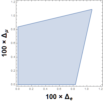
Figure 3: Limits on $\Delta_{r}$ [cf. eq. 29] derived from $W$-mediated decays.

We define $R_{u\rightarrow X}=B(u\rightarrow X)/B_{\tt SM}(u\rightarrow X)-1$; then, for the specific decays of interest, we find (to 3$\sigma$),

$$R_{\tau\rightarrow\mu\nu\bar{\nu}}\simeq B_{\tt SM}(\tau\rightarrow e\nu\bar{\nu})\Delta_{e}-\left[1-B_{\tt SM}(\tau\rightarrow\mu\nu\bar{\nu})\right]\Delta_{\mu} {\quad\Rightarrow\quad}|0.8223\,\Delta_{\mu}-0.1958\,\Delta_{e}|\leq 0.0069\,,$$

$$R_{\tau\rightarrow e\nu\bar{\nu}}\simeq B_{\tt SM}(\tau\rightarrow\mu\nu\bar{\nu})\Delta_{\mu}-\left[1-B_{\tt SM}(\tau\rightarrow e\nu\bar{\nu})\right]\Delta_{e} {\quad\Rightarrow\quad}|0.1777\,\Delta_{\mu}-0.8042\,\Delta_{e}|\leq 0.0067\,,$$

$$R_{\pi\rightarrow\mu\nu}\simeq B_{\tt SM}(\pi\rightarrow e\nu)(\Delta_{\mu}-\Delta_{e}) {\quad\Rightarrow\quad}|\Delta_{\mu}-\Delta_{e}|\leq 0.010\,.$$ (30)

These constraints are summarized in Fig. 3. We note that the limit derived from $\pi\rightarrow\mu e$ is not competitive: $|\Delta_{\mu}-\Delta_{e}|\leq 48.8$. Also, though the uncertainty in $\Gamma(\mu\rightarrow e\nu\bar{\nu})$ is very small, it does not lead to a constraint on $\Delta_{e}+\Delta_{\mu}$, since this decay is used as input data to fix the value of $G_{\tt F}$. One could use collider measurements of $m_{\tt W}$ and $g_{2}$ (the ${SU(2)}_{L}$ coupling constant in the SM) to predict this width, but the uncertainty is much larger and the limits are again not competitive.

3.4 Muon anomalous magnetic moment.

The new $NNW$ vertices, and the ${\cal C}$ factors for the $nnW$ vertices in eq. 8 generate contribution to the anomalous magnetic moment of the muon, $a_{\mu}$. Using the results of  Leveille:1977rc it is straightforward to see that

$$\Delta a_{\mu}=\frac{G_{\tt F}\,m_{\mu}^{2}}{\sqrt{2}\,8\pi^{2}}\Delta_{\mu}\left[F(r_{\tt NW})-F(0)\right]\,,$$ (31)

where $\Delta_{\mu}=\Delta_{r=2}$ is defined in eq. 29 and

$$F(w) =\int_{0}^{1}dx\frac{2x^{2}(1+x)+x(1-x)(2-x)w-x^{2}(x-1)k}{kx^{2}+(1-k)x+(1-x)w}\,;\quad k=\left(\frac{m_{\mu}}{m_{\tt W}}\right)^{2}\,,$$

$$\simeq\int_{0}^{1}dx\frac{2x^{2}(1+x)+x(1-x)(2-x)w}{x+(1-x)w}\,,$$ (32)

so that

$$F(w)-F(0)\simeq\frac{10-33w+45w^{2}-4w^{3}}{6(1-w)^{3}}+\frac{3w^{3}\,\ln w}{(1-w)^{4}}-\frac{5}{3}\,,$$ (33)

and this ranges from $0$ when $w=0$ to $-1$ when $w\rightarrow\infty$. Then

$$|\Delta a_{\mu}|\leq\frac{G_{\tt F}\,m_{\mu}^{2}}{\sqrt{2}\,8\pi^{2}}\Delta_{\mu}=1.17\times 10^{-9}\Delta_{\mu}\,.$$ (34)

The constraints derived form $W$-mediated decays require $\Delta_{\mu}\lesssim 10^{-2}$ (see Fig. 3) so $|\Delta a_{\mu}|\lesssim 10^{-11}$, while the current error Tanabashi:2018oca is $(\pm 5.4\pm 3.3)\times 10^{-10}$. The anomalous magnetic moment limits do not produce a competitive bound now, but may do so with the upgraded Fermilab experiment Grange:2015fou .

4 Relic abundance.

As the universe expands there will come a time when the $\Psi_{\pm}$ will cease to be in chemical equilibrium with the SM or with the dark photon sea. Still, we expect the interactions between $\Psi_{+}$ and $\Psi_{-}$ will keep them in equilibrium with each other and, since they have (approximately) equal mass and couplings with $V$, they will have the same relic abundance; in the following we denote by $n_{\Psi}$ the total DM number density, adding the contributions from the $\Psi_{+}$ and $\Psi_{-}$.

The processes that determine the relic abundance are (see Fig. 4) then $\Psi\bar{\Psi}\rightarrow n_{L}\bar{n}_{L}$ and $\Psi\bar{\Psi}\rightarrow VV$ , for which the cross sections are

$$\sigma_{\Psi\Psi\rightarrow nn} =\frac{\left(z{\cal S}^{2}z^{T}\right)^{2}}{64\pi s\beta_{\Psi}}\left[\frac{1+2y(1+y)-\beta_{\Psi}^{2}}{(1+y)^{2}-\beta_{\Psi}^{2}}+\frac{y}{\beta_{\Psi}}\ln\left(\frac{1-\beta_{\Psi}+y}{1+\beta_{\Psi}-y}\right)\right]\,,$$

$$\sigma_{\Psi\Psi\rightarrow{\tt VV}} =\frac{g^{4}}{8\pi s}\frac{\beta_{\tt V}}{\beta_{\Psi}}\left[\frac{sm_{\Psi}^{2}+4(m_{\tt V}^{4}-2m_{\tt V}^{2}m_{\Psi}^{2}-2m_{\Psi}^{4})}{sm_{\Psi}^{2}+m_{\tt V}^{2}(m_{\tt V}^{2}-4m_{\Psi}^{2})}+\frac{4(m_{\tt V}^{2}+m_{\Psi}^{2})}{s\beta_{\tt V}\beta_{\Psi}}\ln\left|\frac{1+\beta_{\tt V}^{2}+2\beta_{\Psi}\beta_{\tt V}}{1+\beta_{\tt V}^{2}-2\beta_{\Psi}\beta_{\tt V}}\right|\right]\,,$$ (35)

where

$$y=\frac{2(m_{\Phi}^{2}-m_{\Psi}^{2})}{s}\,;\qquad\beta_{\Psi}=\sqrt{1-\frac{4m_{\Psi}^{2}}{s}}\,;\qquad\beta_{\tt V}=\sqrt{1-\frac{4m_{\tt V}^{2}}{s}}\,.$$ (36)

Figure 4: Diagrams giving the leading contributions to the relic abundance cross sections.

Since we are considering DM masses smaller than those for the $Z$ and $H$, there will be no resonant contributions to the relic abundance calculations, and the usual approximations Kolb:1990vq can be reliably used. After a straightforward calculation we find

$$\left\langle{\rm v}\,\sigma_{\Psi\Psi\rightarrow nn}\right\rangle \simeq\frac{\left(z{\cal S}^{2}z^{T}\right)^{2}}{32\pi(r_{{\tt\Psi}{\tt\Phi}}+1)^{2}m_{\Psi}^{2}}\,,$$

$$\left\langle{\rm v}\,\sigma_{\Psi\Psi\rightarrow{\tt VV}}\right\rangle \simeq\frac{g^{4}}{16\pi m_{\Psi}^{2}}\,,$$ (37)

where we summed over all final neutrino states and took $m_{\Psi}\gg m_{\tt V}$ (cf. eq. 16); since there is no temperature dependence to lowest order, these are s-wave reactions.

We follow the usual prescription for abundance calculation via the Boltzmann Equation:

$$\frac{dn_{\Psi}}{dt}+3Hn_{\Psi}=-\sigma_{0}\left[n_{\Psi}^{2}-\left(n_{\Psi}^{\left(\tt eq\right)}\right)^{2}\right]\,,$$ (38)

where

$$\sigma_{0}=\frac{1}{2}\left\langle{\rm v}\,\sigma_{\Psi\Psi\rightarrow nn}\right\rangle+\frac{1}{4}\left\langle{\rm v}\,\sigma_{\Psi\Psi\rightarrow{\tt VV}}\right\rangle=\frac{g^{4}+\left[z{\cal S}^{2}z^{T}/(r_{{\tt\Psi}{\tt\Phi}}+1)\right]^{2}}{64\pi m_{\Psi}^{2}}\,.$$ (39)

Using the standard freeze-out approximation  Kolb:1990vq , the relic abundance $\Omega_{\Psi}$ is given by:

$$\Omega_{\Psi}h^{2}=\frac{1.07\times 10^{9}}{\hbox{GeV}}\frac{x_{f}}{{\tt g}_{\star\tt s}\xi}\,;\quad\xi=\frac{M_{\rm Pl}\sigma_{0}}{\sqrt{{\tt g}_{\star}}}$$ (40)

where $M_{\rm Pl}$ denotes the Planck mass, ${\tt g}_{\star\tt s},\,{\tt g}_{\star}$ denote, respectively, the relativistic degrees of freedom associated with the entropy and energy density  (for our case they are the same), and

$$x_{f}=\frac{m_{\Psi}}{T_{f}}=\ln\left(0.076m_{\Psi}\xi\right)-\frac{1}{2}\ln\left[\ln\left(0.076m_{\Psi}\xi\right)\right]\,,$$ (41)

with $T_{f}$ the freeze-out temperature. This expression for $\Omega_{\Psi}$ can now be compared to the result inferred from CMB data obtained by the Planck experiment Aghanim:2018eyx ; Ade:2015xua :

$$\Omega_{\rm Planck}h^{2}=0.12\pm 0.003\quad(3\sigma).$$ (42)

Note, in particular, that a sufficiently large value of the dark-photon coupling $g$ will lead to DM under-abundance.

5 Direct Detection

In the model under consideration the DM-nucleon scattering cross section responsible for a direct detection signal is generated by (t-channel) $Z$ and $H$ exchanges associated with the loop-induced couplings listed in Sect. 2.1. Since the momentum transfer is much smaller than $m_{\tt Z}$ and $m_{\tt H}$ we can approximate the relevant interaction by

$${\cal L}_{\tt nucleon-DM}=\sqrt{2}G_{\tt F}\,\left[\bar{\Psi}\gamma_{\mu}\left(\epsilon_{L}P_{L}+\epsilon_{R}P_{R}\right)\Psi\right]\,\left(\bar{\mathfrak{p}}{\cal J}^{\mu}_{\mathfrak{p}}{\mathfrak{p}}+\bar{\mathfrak{n}}{\cal J}^{\mu}_{\mathfrak{n}}{\mathfrak{n}}\right)+G_{\tt H}\bar{\Psi}\Psi\left(\bar{\mathfrak{p}}{\mathfrak{p}}+\bar{\mathfrak{n}}{\mathfrak{n}}\right)\,,$$ (43)

where ${\mathfrak{p}},\,{\mathfrak{n}}$ denote, respectively, the proton and neutron fields and  Engel:1991wq

$${\cal J}^{\mu}_{\mathfrak{p}} =\frac{1}{2}\left[\left(1-4s_{\tt W}^{2}\right)\gamma^{\mu}+g_{A}\left(\gamma^{\mu}-\frac{2m_{\cal N}q^{\mu}}{m_{\pi}^{2}+{\bf q}^{2}}\right)\gamma_{5}\right]\,,$$

$${\cal J}^{\mu}_{\mathfrak{n}} =-\frac{1}{2}\left[\gamma^{\mu}+g_{A}\left(\gamma^{\mu}-\frac{2m_{\cal N}q^{\mu}}{m_{\pi}^{2}+{\bf q}^{2}}\right)\gamma_{5}\right]\,,$$ (44)

with $m_{\cal N},\,m_{\pi}$ the nucleon and pion masses, ${\bf q}$ the momentum transfer, $g_{A}\simeq-1.2723$ the axial nucleon coupling Tanabashi:2018oca , and Cheng:2014opa

$$G_{\tt H}=-\frac{0.011\epsilon_{H}}{m_{\tt H}^{2}}\,.$$ (45)

All isospin breaking effects in the Higgs-mediated interactions were ignored.

In the non-relativistic limit this becomes

$$\frac{1}{m_{\Psi}m_{\cal N}}\left.{\cal L}_{\tt nucleon-DM}\right|_{\tt NR}= 4G_{H}{\mathbbm{1}}_{\Psi}\,{\mathbbm{1}}_{\cal N}+\sqrt{2}\,G_{\tt F}(\epsilon_{R}+\epsilon_{L})\Biggl{\{}\left[-2s_{\tt W}^{2}+(1-2s_{\tt W}^{2})]\tau_{3}\right]{\mathbbm{1}}_{\Psi}\,{\mathbbm{1}}_{\cal N}$$

$$\qquad\qquad+\tau_{3}\left[{\bf s}_{\Psi}.{\bf s}_{\cal N}-4\frac{({\bf q}.{\bf s}_{\Psi})({\bf q}.{\bf s}_{\cal N})}{m_{\pi}^{2}+{\bf q}^{2}}\right]\left(\frac{\epsilon_{R}-\epsilon_{L}}{\epsilon_{R}+\epsilon_{L}}\right)g_{A}\Biggr{\}}\,,$$ (46)

where $\tau_{3}\rightarrow 1$ for ${\mathfrak{p}}$ and $\tau_{3}\rightarrow-1$ for ${\mathfrak{n}}$, ${\bf s}_{\Psi,\,{\cal N}}$ denote the spin operators for the DM and the nucleons. Using the notation and procedure described in Fitzpatrick:2012ix ; Anand:2014kea (see also Walecka:1975 ) we find that the DM-nucleus cross section, which we denote by $\sigma_{\cal A}$ is given by

$$\sigma_{\cal A} =\frac{(m_{\cal A}/m_{\cal N})^{2}}{16\pi(m_{\cal A}+m_{\Psi})^{2}}\biggl{\{}\kappa^{2}\left[(1+b)^{2}F_{M}^{\left({\mathfrak{p}},{\mathfrak{p}}\right)}+(1-b)^{2}F_{M}^{\left({\mathfrak{n}},{\mathfrak{n}}\right)}+2(1-b^{2})F_{M}^{\left({\mathfrak{p}},{\mathfrak{n}}\right)}\right]$$

$$\quad+\frac{{\mathbbm{K}}^{2}(Q^{2}-2Q+3)}{12}\left[F_{\Sigma^{\prime\prime}}^{\left({\mathfrak{p}},{\mathfrak{p}}\right)}+F_{\Sigma^{\prime\prime}}^{\left({\mathfrak{n}},{\mathfrak{n}}\right)}-2F_{\Sigma^{\prime\prime}}^{\left({\mathfrak{p}},{\mathfrak{n}}\right)}+2\left(F_{\Sigma^{\prime}}^{\left({\mathfrak{p}},{\mathfrak{p}}\right)}+F_{\Sigma^{\prime}}^{\left({\mathfrak{n}},{\mathfrak{n}}\right)}-2F_{\Sigma^{\prime}}^{\left({\mathfrak{p}},{\mathfrak{n}}\right)}\right)\right]\biggr{\}}\,,$$ (47)

where ${\cal A}$ is the atomic number, $m_{\cal A}\simeq{\cal A}m_{\cal N}$ the nuclear mass, and

$$\kappa=\sqrt{2}G_{\tt F}m_{\Psi}m_{\cal N}\left[2(\epsilon_{L}+\epsilon_{R})s_{\tt W}^{2}-2\sqrt{2}\,\frac{G_{\tt H}}{G_{\tt F}}\right]\,,\quad Q=\frac{4|{\bf q}|^{2}}{|{\bf q}|^{2}+m_{\pi}^{2}}\,,$$

$${\mathbbm{K}}=\frac{G_{\tt F}(\epsilon_{R}-\epsilon_{L})m_{\Psi}m_{\cal N}}{\sqrt{2}}g_{A}\,,\quad b=\frac{1-2s_{\tt W}^{2}}{\sqrt{8}G_{\tt H}/[(\epsilon_{L}+\epsilon_{R})G_{\tt F}]-2s_{\tt W}^{2}}\,.$$ (48)

The DM-nucleon cross section is then defined Fitzpatrick:2012ix ; Lewin:1995rx as

$$\sigma_{N}=\left(\frac{m_{\cal N}}{m_{\cal A}}\right)^{2}\left(\frac{m_{\Psi}+m_{\cal A}}{m_{\Psi}+m_{\cal N}}\right)^{2}\frac{1}{{\cal A}^{2}}\sigma_{\cal A}\,.$$ (49)

If there are several isotopes, labeled by $I$, with abundances $\alpha_{I}$, then $F_{X}^{\left(N,N^{\prime}\right)}\rightarrow\,^{I}F_{X}^{\left(N,N^{\prime}\right)}$ and

$$\frac{1}{{\cal A}^{2}}F_{X}^{\left(N,N^{\prime}\right)}\rightarrow\sum_{I}\frac{\alpha_{I}}{{\cal A}_{I}^{2}}\;^{I}F_{X}^{\left(N,N^{\prime}\right)}=f_{X}^{\left(N,N^{\prime}\right)}\,;$$ (50)

so, defining

$$f_{1}= f_{M}^{\left({\mathfrak{p}},{\mathfrak{p}}\right)}+f_{M}^{\left({\mathfrak{n}},{\mathfrak{n}}\right)}+2f_{M}^{\left({\mathfrak{p}},{\mathfrak{n}}\right)}\,,$$

$$f_{2}= f_{M}^{\left({\mathfrak{p}},{\mathfrak{p}}\right)}-f_{M}^{\left({\mathfrak{n}},{\mathfrak{n}}\right)}\,,$$

$$f_{3}= f_{M}^{\left({\mathfrak{p}},{\mathfrak{p}}\right)}+f_{M}^{\left({\mathfrak{n}},{\mathfrak{n}}\right)}-2f_{M}^{\left({\mathfrak{p}},{\mathfrak{n}}\right)}\,,$$

$$f_{4}= \left(f_{\Sigma^{\prime\prime}}^{\left({\mathfrak{p}},{\mathfrak{p}}\right)}+f_{\Sigma^{\prime\prime}}^{\left({\mathfrak{n}},{\mathfrak{n}}\right)}-2f_{\Sigma^{\prime\prime}}^{\left({\mathfrak{p}},{\mathfrak{n}}\right)}\right)+\left(f_{\Sigma^{\prime}}^{\left({\mathfrak{p}},{\mathfrak{p}}\right)}+f_{\Sigma^{\prime}}^{\left({\mathfrak{n}},{\mathfrak{n}}\right)}-2f_{\Sigma^{\prime}}^{\left({\mathfrak{p}},{\mathfrak{n}}\right)}\right)\,,$$ (51)

the expression for the DM-nucleon cross section takes the relatively simple form

$$\sigma_{\cal N}=\frac{1}{16\pi^{2}(m_{\cal N}+m_{\Psi})^{2}}\left[\left(f_{1}+2bf_{2}+b^{2}f_{3}\right)\kappa^{2}+\frac{{\mathbbm{K}}^{2}(Q^{2}-2Q+3)}{12}f_{4}\right]\,.$$ (52)

It is worth noting that the term $\propto\kappa^{2}$ is the spin-independent contribution, while that $\propto{\mathbbm{K}}^{2}$ is the spin-dependent one. The expected suppression of the latter with respect to the former follows from $f_{4}\ll f_{1}$. In the calculations we use the expressions for the ${}^{I}F_{X}^{\left(N,N^{\prime}\right)}$ provided in Fitzpatrick:2012ix for Xe and Ge, and in Catena:2015uha   for CaWO₄:

$$\begin{array}[]{c||c|c|c|c}\text{element}&f_{1}&f_{2}&f_{3}&f_{4}\times 10^{4}\cr\hline\cr\text{Xe}&0.995256-6.98794{\bf q}^{2}&-0.177925+1.39348{\bf q}^{2}&0.031717-0.314739{\bf q}^{2}&0.142261-1.22925{\bf q}^{2}\cr\text{Ge}&0.990137-6.97097{\bf q}^{2}&-0.124142+0.960981{\bf q}^{2}&0.0161359-0.115939{\bf q}^{2}&0.156404-1.61629{\bf q}^{2}\cr\text{CaWO}_{4}&0.0624983-0.447775{\bf q}^{2}&0&0&0\end{array}$$ (53)

and we took $|{\bf q}|=m_{\Psi}\times 300$km/s.

We note that the dependence of $\sigma_{\cal N}$ on $m_{\Psi}$ is simple and contained in the factor $[m_{\Psi}/(m_{\Psi}+m_{\cal N})]^{2}$, it also has a more complicated dependence on $m_{\Phi},\,m_{\tt N}$ through the parameters $\epsilon_{L,\,R,\,H}$.

In the numerical results below we used the experimental constraints on the direct detection cross section published by Xenon1T Aprile:2019dbj , PandaX Cui:2017nnn , CDMS Agnese:2013rvf and CRESST Abdelhameed:2019hmk for the range $0.36\,\hbox{GeV}\leq m_{\Psi}\leq 10\,\hbox{GeV}$; in cases where the mass ranges of two experiments overlap we take the strictest limit. Specifically, we used:

$$\begin{array}[]{|l|rl|}\text{Experiment}&\vrule\lx@intercol\hfil m_{\Psi}\text{ range (GeV)}\hfil\lx@intercol\vrule\lx@intercol\cr\hline\cr\text{Xenon1T}&\quad(6.06,&10.0)\cr\text{PandaX}&(4.12,&6.06)\cr\text{CDMS}&(1.61,&4.12)\cr\text{CRESST}&(0.36,&1.61)\end{array}$$ (54)

as illustrated in Fig. 6.

6 Numerical Results

The model being considered has in total 14 free parameters: $m_{\Psi}$, $\mu$, $m_{\Phi}$, $m_{\tt N}$, $\lambda_{x}$, ${\cal S}$ and $z$ (we assumed $m_{\tt V}$ and $g$ are fixed by eqs. 16 and 17). We will for simplicity assume that $z$ is real since all the observables we consider depend only on the magnitudes $z_{i}$, this reduces the number of parameters to 10. In this section we consider the region in parameter space

$$0.5\hbox{GeV}\leq m_{\Psi}\leq 10\hbox{GeV}\,,\qquad\mu=\frac{m_{\Psi}}{20}\,,$$

$$\text{min}\{1.1m_{\Psi},\,m_{\Psi}+2\hbox{GeV}\}\leq m_{\Phi}<500\hbox{GeV}\,,$$

$$\text{min}\{1.1m_{\Psi},\,m_{\Psi}+2\hbox{GeV}\}\leq m_{\tt N}\leq 1.5\hbox{TeV}\,,$$

$$|\lambda_{x}|\leq\pi\,,\quad|S_{i}|<1\,,\quad|z_{i}|^{2}\leq 10\quad(i=1,2,3);$$ (55)

and determine the sub-region allowed by the various constraints listed above. This is frequently carried out by reducing the number of free parameters (e.g. fixing the ${\cal S}$ and taking all the $z_{i}$ equal Gonzalez-Macias:2016vxy ) and then doing a uniform scan in the reduced space. Here we follow a different route: we do not adopt any simplifying relations between the parameters (except $\mu$), and concentrate on finding the boundary of the allowed sub-region; this then becomes a non-linear optimization problem that can be treated using standard techniques Pierre:1986 . In our calculations we use a publicly-available non-linear programming package NLOPT Johnson:NLOPT .

$$\begin{array}[]{ccc}\includegraphics[scale={0.6}]{figs/MPhi.png}&&\includegraphics[scale={0.6}]{figs/lx.png}\cr(a)&&(b)\vspace{20pt}\cr\includegraphics[scale={0.6}]{figs/z.png}&&\includegraphics[scale={0.6}]{figs/mix.png}\cr(c)&&(d)\end{array}$$

Figure 5: Projections of the allowed parameter region, $(a)$ in the $m_{\Psi}-m_{\Phi}$ plane, $(b)$ the $\lambda_{x}-m_{\Phi}$ plane, $(c)$ the $m_{\Psi}-\left\langle z\right\rangle$ plane (where $\left\langle z\right\rangle=|z|/\sqrt{3}$), and $(d)$ the $m_{\Psi}-\left\langle\text{mix}\right\rangle$ plane, where $\left\langle\text{mix}\right\rangle$ is defined in eq. 56. The unevenness in the curves are due to numerical inaccuracies.

We define

$$\left\langle\text{mix}\right\rangle=\sum|z_{i}|^{2}{\cal S}_{i}^{2}\,,\quad\left\langle z\right\rangle=|z|/\sqrt{3}\,,$$ (56)

as measures of the mixing strength and Yukawa coupling of the mediators, and then obtain the projections of the allowed sub-region in the $m_{\Psi}-m_{\Phi}$, $m_{\Psi}-\lambda_{x}$, $m_{\Psi}-\left\langle z\right\rangle$ and the $m_{\Psi}-\left\langle\text{mix}\right\rangle$ planes. The results are presented in Figs. 5 $(a)-(d)$ respectively. In the $m_{\Psi}-m_{\tt N}$ plane the constraints allow the full area indicated in eq. 55; that is, for each point in this area there are values of the other parameters for which all constraints are satisfied (in general these values change for each choice of $m_{\Psi}$ and $m_{\tt N}$). The features in figures $(b),\,(c),\,(d)$ at $m_{\Psi}\sim 4\,\hbox{GeV}$ and $m_{\Psi}\sim 6\,\hbox{GeV}$ are due to the changes in the constraints of the direct-detection cross section (cf. eq. 54).

      

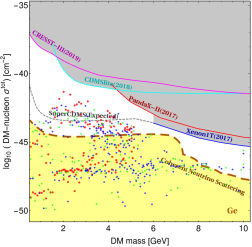
Figure 6: Experimental limits on the direct detection cross section $\sigma$. The upper curves are obtained, from left to right, from the CRESST, CDMS, PandaX and Xenon1T experiments, and the expected sensitivity limit for the superCDMS experiment Agnese:2016cpb ; the coherent neutrino scattering regions are calculated for Xe (left) and Ge (right). For illustration we also include the cross sections corresponding to a selection of points on the boundary of the allowed region of parameter space, on the upper and lower boundaries of Fig. 5(a) (green points), of Fig. 5(c) (red points), and of Fig. 5(d) (blue points).

In Fig. 6 we plot the values of the direct-detection cross sections for a selection of points on or close to the boundary of the allowed region of parameter space. The points are chosen only to illustrate that there is a region of parameter space within the sensitivity reach of SuperCDMS Agnese:2016cpb , but that this experiment cannot exclude the model; it is also worth noting that a (different) region of parameter space will correspond to cross sections above the coherent neutrino scattering ‘floor’. Both these regions are significant in size: restricting the model to either (or both) would not require fine tuning.

7 Conclusions

In this paper, we have considered an extension of the neutrino-portal DM scenario, introducing strong interactions to the dark sector via a $U(1)_{\tt dark}$ local symmetry with its corresponding vector boson $V$. The dark sector consists of a scalar $\Phi$, the dark photon $V$, and two almost degenerate fermions $\Psi_{\pm}$, of opposite $U(1)_{\tt dark}$ charges and which constitute the DM relics. We have also imposed a (softly broken) $\mathbb{Z}_{2}$ dark-charge symmetry that strongly suppresses $V$ mixings with the SM photon and $Z$, but still allows for the $V$ to decay into neutrinos with a sufficiently short lifetime, as required by phenomenology; this imposes mild constraints on the soft breaking parameter. These modifications to the model preserve the naturally small direct and indirect detection cross sections and the relatively large annihilation cross-sections without fine-tuning.

The core vs. cusp data in galaxies and clusters place a limit on the DM self-interaction cross sections, from which we derive limits on the strong interaction coupling and the mass of the $V$ boson. The presence of oppositely charged DM components opens the possibility that bound states are formed; if this occurs, and the formation of rate such bound states is sufficiently high the core vs. cusp problem would reappear as the interactions between the bound states will be weak (akin to the Van der Waals interactions). In this paper we took a conservative approach and simply required that the potential generated by the $V$ should not lead to $[\Psi_{\!+}\!\Psi_{\!-}]$ bound states by assuming that these particles are sufficiently light, accordingly we have chosen $m_{\Psi}\lesssim O(10\,\hbox{GeV})$ in our numerical calculations; we will return to the issue of bound state formation in a future publication.

The relic density constraint also imposes strong restrictions on the model. Specifically, a large dark photon coupling $g$ leads (cf. eq. 39) to under-production of DM, so the upper allowed values (see eqs. 16 and 17) for this coupling are generally problematic. A more precise determination of the DM cross section as a function of velocity will provide a strict test of the viability of this model. In addition, $Z$ and $W$ data, impose important restrictions on the mixing angles ${\cal S}$ and Yukawa couplings $z$.

Other constraints on the model are milder. For example, the DM-nucleon cross section is naturally suppressed in this model (it is a one-loop effect), so that the direct-detection limits provide less significant in restrictions than in other models. We have not included constraints derived from neutrino oscillations because they are not precise enough to provide significant limits. The same applies to existing limits derived from the measurement of the muon anomalous magnetic moment, in this case, however, an improvement by one order of magnitude in the experimental sensitivity would provide useful constraints on this model.

As with the original model Gonzalez-Macias:2016vxy , the most distinct detection signature would come from the annihilation of $\Psi$’s into neutrinos, producing a monochromatic neutrino line from both the sun and the galactic halo; unfortunately, current detection experiments have insufficient sensitivity to detect such a signal.

Also of interest are the allowed values of the mass of the dark scalars, $m_{\Psi}<m_{\Phi}\lesssim 300\,\hbox{GeV}$ (Fig. 5 $(a)$). The existence of this particle can be probed in principle by accurate measurements of the cosmological or astrophysical neutrino flux, since it will exhibit a resonance at neutrino energy $E_{\nu}^{\left(\tt res\right)}=(m_{\Phi}^{2}-m_{\Psi}^{2})/(2m_{\Psi})$ in the scattering of high-energy neutrinos off the ambient DM. Numerically, $E_{\nu}^{\left(\tt res\right)}\sim 3.7\,\hbox{TeV}$ (roughly independent of $m_{\Psi}$) for the maximum allowed values of $m_{\Phi}$ (upper boundary in the figure). Observation of this effect is challenging because the atmospheric neutrino flux is much larger at these energies.

The presence of a dark photon generates a significant change from the previous model Gonzalez-Macias:2016vxy . The dark photons are long-lived and will decay into neutrinos; possible effects of these decays will be explored in a future publication.

References

- (1) F. Zwicky, Die Rotverschiebung von extragalaktischen Nebeln, Helv. Phys. Acta 6 (1933) 110.
- (2) V. C. Rubin and W. K. Ford, Jr., Rotation of the Andromeda Nebula from a Spectroscopic Survey of Emission Regions, Astrophys. J. 159 (1970) 379.
- (3) E. Corbelli and P. Salucci, The Extended Rotation Curve and the Dark Matter Halo of M33, Mon. Not. Roy. Astron. Soc. 311 (2000) 441 [astro-ph/9909252].
- (4) S. W. Allen, A. E. Evrard and A. B. Mantz, Cosmological Parameters from Observations of Galaxy Clusters, Ann. Rev. Astron. Astrophys. 49 (2011) 409 [1103.4829].
- (5) D. Clowe, M. Bradac, A. H. Gonzalez, M. Markevitch, S. W. Randall, C. Jones et al., A direct empirical proof of the existence of dark matter, Astrophys. J. 648 (2006) L109 [astro-ph/0608407].
- (6) NASA PICO collaboration, PICO: Probe of Inflation and Cosmic Origins, 1902.10541.
- (7) E. Behnke et al., Final Results of the PICASSO Dark Matter Search Experiment, Astropart. Phys. 90 (2017) 85 [1611.01499].
- (8) PandaX-II collaboration, Spin-Dependent Weakly-Interacting-Massive-Particle–Nucleon Cross Section Limits from First Data of PandaX-II Experiment, Phys. Rev. Lett. 118 (2017) 071301 [1611.06553].
- (9) LUX collaboration, Results on the Spin-Dependent Scattering of Weakly Interacting Massive Particles on Nucleons from the Run 3 Data of the LUX Experiment, Phys. Rev. Lett. 116 (2016) 161302 [1602.03489].
- (10) XENON collaboration, First Dark Matter Search Results from the XENON1T Experiment, Phys. Rev. Lett. 119 (2017) 181301 [1705.06655].
- (11) LUX collaboration, Results from a search for dark matter in the complete LUX exposure, Phys. Rev. Lett. 118 (2017) 021303 [1608.07648].
- (12) PandaX-II collaboration, Dark Matter Results from First 98.7 Days of Data from the PandaX-II Experiment, Phys. Rev. Lett. 117 (2016) 121303 [1607.07400].
- (13) E. Bulbul, M. Markevitch, A. Foster, R. K. Smith, M. Loewenstein and S. W. Randall, Detection of An Unidentified Emission Line in the Stacked X-ray spectrum of Galaxy Clusters, Astrophys. J. 789 (2014) 13 [1402.2301].
- (14) O. Ruchayskiy, A. Boyarsky, D. Iakubovskyi, E. Bulbul, D. Eckert, J. Franse et al., Searching for decaying dark matter in deep XMM?Newton observation of the Draco dwarf spheroidal, Mon. Not. Roy. Astron. Soc. 460 (2016) 1390 [1512.07217].
- (15) J. Franse et al., Radial Profile of the 3.55 keV line out to in the Perseus Cluster, Astrophys. J. 829 (2016) 124 [1604.01759].
- (16) O. Urban, N. Werner, S. W. Allen, A. Simionescu, J. S. Kaastra and L. E. Strigari, A Suzaku Search for Dark Matter Emission Lines in the X-ray Brightest Galaxy Clusters, Mon. Not. Roy. Astron. Soc. 451 (2015) 2447 [1411.0050].
- (17) Hitomi collaboration, constraints on the 3.5 keV line in the Perseus galaxy cluster, Astrophys. J. 837 (2017) L15 [1607.07420].
- (18) Super-Kamiokande collaboration, Search for neutrinos from annihilation of captured low-mass dark matter particles in the Sun by Super-Kamiokande, Phys. Rev. Lett. 114 (2015) 141301 [1503.04858].
- (19) IceCube collaboration, Search for annihilating dark matter in the Sun with 3 years of IceCube data, Eur. Phys. J. C77 (2017) 146 [1612.05949].
- (20) Fermi-LAT collaboration, The Fermi Galactic Center GeV Excess and Implications for Dark Matter, Astrophys. J. 840 (2017) 43 [1704.03910].
- (21) D. Hooper and L. Goodenough, Dark Matter Annihilation in The Galactic Center As Seen by the Fermi Gamma Ray Space Telescope, Phys. Lett. B697 (2011) 412 [1010.2752].
- (22) Fermi-LAT collaboration, Searching for Dark Matter Annihilation from Milky Way Dwarf Spheroidal Galaxies with Six Years of Fermi Large Area Telescope Data, Phys. Rev. Lett. 115 (2015) 231301 [1503.02641].
- (23) M.-Y. Cui, Q. Yuan, Y.-L. S. Tsai and Y.-Z. Fan, Possible dark matter annihilation signal in the AMS-02 antiproton data, Phys. Rev. Lett. 118 (2017) 191101 [1610.03840].
- (24) ATLAS collaboration, Dark matter interpretations of ATLAS searches for the electroweak production of supersymmetric particles in TeV proton-proton collisions, JHEP 09 (2016) 175 [1608.00872].
- (25) CMS collaboration, Search for dark matter in events with energetic, hadronically decaying top quarks and missing transverse momentum at TeV, JHEP 06 (2018) 027 [1801.08427].
- (26) D. Abercrombie et al., Dark Matter Benchmark Models for Early LHC Run-2 Searches: Report of the ATLAS/CMS Dark Matter Forum, 1507.00966.
- (27) W. J. G. de Blok, The Core-Cusp Problem, Adv. Astron. 2010 (2010) 789293 [0910.3538].
- (28) R. A. Flores and J. R. Primack, Observational and theoretical constraints on singular dark matter halos, Astrophys. J. 427 (1994) L1 [astro-ph/9402004].
- (29) B. Moore, Evidence against dissipationless dark matter from observations of galaxy haloes, Nature 370 (1994) 629.
- (30) B. Moore, T. R. Quinn, F. Governato, J. Stadel and G. Lake, Cold collapse and the core catastrophe, Mon. Not. Roy. Astron. Soc. 310 (1999) 1147 [astro-ph/9903164].
- (31) D. N. Spergel and P. J. Steinhardt, Observational evidence for selfinteracting cold dark matter, Phys. Rev. Lett. 84 (2000) 3760 [astro-ph/9909386].
- (32) S. Tulin and H.-B. Yu, Dark Matter Self-interactions and Small Scale Structure, Phys. Rept. 730 (2018) 1 [1705.02358].
- (33) V. González-Macías, J. I. Illana and J. Wudka, A realistic model for Dark Matter interactions in the neutrino portal paradigm, JHEP 05 (2016) 171 [1601.05051].
- (34) V. González-Macías, J. Illana and J. Wudka, Dark matter and the neutrino portal paradigm, J. Phys. Conf. Ser. 761 (2016) 012082 [1608.06267].
- (35) N. Cosme, L. Lopez Honorez and M. H. G. Tytgat, Leptogenesis and dark matter related?, Phys. Rev. D72 (2005) 043505 [hep-ph/0506320].
- (36) A. Falkowski, J. Juknevich and J. Shelton, Dark Matter Through the Neutrino Portal, 0908.1790.
- (37) H. An, S.-L. Chen, R. N. Mohapatra and Y. Zhang, Leptogenesis as a Common Origin for Matter and Dark Matter, JHEP 03 (2010) 124 [0911.4463].
- (38) M. Lindner, A. Merle and V. Niro, Enhancing Dark Matter Annihilation into Neutrinos, Phys. Rev. D82 (2010) 123529 [1005.3116].
- (39) A. Falkowski, J. T. Ruderman and T. Volansky, Asymmetric Dark Matter from Leptogenesis, JHEP 05 (2011) 106 [1101.4936].
- (40) Y. Farzan, Flavoring Monochromatic Neutrino Flux from Dark Matter Annihilation, JHEP 02 (2012) 091 [1111.1063].
- (41) J. Heeck and H. Zhang, Exotic Charges, Multicomponent Dark Matter and Light Sterile Neutrinos, JHEP 05 (2013) 164 [1211.0538].
- (42) S. Baek, P. Ko and W.-I. Park, Singlet Portal Extensions of the Standard Seesaw Models to a Dark Sector with Local Dark Symmetry, JHEP 07 (2013) 013 [1303.4280].
- (43) I. Baldes, N. F. Bell, A. J. Millar and R. R. Volkas, Asymmetric Dark Matter and CP Violating Scatterings in a UV Complete Model, JCAP 1510 (2015) 048 [1506.07521].
- (44) B. Batell, T. Han and B. Shams Es Haghi, Indirect Detection of Neutrino Portal Dark Matter, Phys. Rev. D97 (2018) 095020 [1704.08708].
- (45) S. HajiSadeghi, S. Smolenski and J. Wudka, Asymmetric dark matter with a possible Bose-Einstein condensate, Phys. Rev. D99 (2019) 023514 [1709.00436].
- (46) A. Berlin and N. Blinov, A Thermal Neutrino Portal to Sub-MeV Dark Matter, 1807.04282.
- (47) P. Bandyopadhyay, E. J. Chun, R. Mandal and F. S. Queiroz, Scrutinizing Right-Handed Neutrino Portal Dark Matter With Yukawa Effect, Phys. Lett. B788 (2019) 530 [1807.05122].
- (48) M. Blennow, E. Fernandez-Martinez, A. O.-D. Campo, S. Pascoli, S. Rosauro-Alcaraz and A. V. Titov, Neutrino Portals to Dark Matter, 1903.00006.
- (49) B. Holdom, Two U(1)’s and Epsilon Charge Shifts, Phys. Lett. 166B (1986) 196.
- (50) J. Alexander et al., Dark Sectors 2016 Workshop: Community Report, 2016, 1608.08632, http://lss.fnal.gov/archive/2016/conf/fermilab-conf-16-421.pdf.
- (51) D. Wyler and L. Wolfenstein, Massless Neutrinos in Left-Right Symmetric Models, Nucl. Phys. B218 (1983) 205.
- (52) R. N. Mohapatra and J. W. F. Valle, Neutrino Mass and Baryon Number Nonconservation in Superstring Models, Phys. Rev. D34 (1986) 1642.
- (53) E. Ma, Lepton Number Nonconservation in Superstring Models, Phys. Lett. B191 (1987) 287.
- (54) M. Kaplinghat, S. Tulin and H.-B. Yu, Dark Matter Halos as Particle Colliders: Unified Solution to Small-Scale Structure Puzzles from Dwarfs to Clusters, Phys. Rev. Lett. 116 (2016) 041302 [1508.03339].
- (55) B. Ahlgren, T. Ohlsson and S. Zhou, Comment on ?Is Dark Matter with Long-Range Interactions a Solution to All Small-Scale Problems of ? Cold Dark Matter Cosmology??, Phys. Rev. Lett. 111 (2013) 199001 [1309.0991].
- (56) Y. Zhang, Long-lived Light Mediator to Dark Matter and Primordial Small Scale Spectrum, JCAP 1505 (2015) 008 [1502.06983].
- (57) H. An, M. B. Wise and Y. Zhang, Effects of Bound States on Dark Matter Annihilation, Phys. Rev. D93 (2016) 115020 [1604.01776].
- (58) J. P. Edwards, U. Gerber, C. Schubert, M. A. Trejo and A. Weber, The Yukawa potential: ground state energy and critical screening, Progress of Theoretical and Experimental Physics 2017 (2017) [http://oup.prod.sis.lan/ptep/article-pdf/2017/8/083A01/19576961/ptx107.pdf].
- (59) H. Baer, K.-Y. Choi, J. E. Kim and L. Roszkowski, Dark matter production in the early Universe: beyond the thermal WIMP paradigm, Phys. Rept. 555 (2015) 1 [1407.0017].
- (60) Particle Data Group collaboration, Review of Particle Physics, Phys. Rev. D98 (2018) 030001.
- (61) J. P. Leveille, The Second Order Weak Correction to (G-2) of the Muon in Arbitrary Gauge Models, Nucl. Phys. B137 (1978) 63.
- (62) Muon g-2 collaboration, Muon (g-2) Technical Design Report, 1501.06858.
- (63) R. H. Parker, C. Yu, W. Zhong, B. Estey and H. M ller, Measurement of the fine-structure constant as a test of the Standard Model, Science 360 (2018) 191 [1812.04130].
- (64) E. W. Kolb and M. S. Turner, The Early Universe, Front. Phys. 69 (1990) 1.
- (65) P. Gondolo and G. Gelmini, Cosmic abundances of stable particles: Improved analysis, Nucl. Phys. B360 (1991) 145.
- (66) Planck collaboration, Planck 2018 results. VI. Cosmological parameters, 1807.06209.
- (67) Planck collaboration, Planck 2015 results. XIII. Cosmological parameters, Astron. Astrophys. 594 (2016) A13 [1502.01589].
- (68) HERMES collaboration, Precise determination of the spin structure function g(1) of the proton, deuteron and neutron, Phys. Rev. D75 (2007) 012007 [hep-ex/0609039].
- (69) Compass collaboration, Spin asymmetry A1(d) and the spin-dependent structure function g1(d) of the deuteron at low values of x and Q**2, Phys. Lett. B647 (2007) 330 [hep-ex/0701014].
- (70) F. E. Maas and K. D. Paschke, Strange nucleon form-factors, Prog. Part. Nucl. Phys. 95 (2017) 209.
- (71) J. Engel, Nuclear form-factors for the scattering of weakly interacting massive particles, Phys. Lett. B264 (1991) 114.
- (72) H.-Y. Cheng, Scalar and Pseudoscalar Higgs Couplings with Nucleons, Nucl. Phys. Proc. Suppl. 246-247 (2014) 109.
- (73) A. L. Fitzpatrick, W. Haxton, E. Katz, N. Lubbers and Y. Xu, The Effective Field Theory of Dark Matter Direct Detection, JCAP 1302 (2013) 004 [1203.3542].
- (74) N. Anand, A. L. Fitzpatrick and W. C. Haxton, Model-independent Analyses of Dark-Matter Particle Interactions, Phys. Procedia 61 (2015) 97 [1405.6690].
- (75) J. Walecka, Semileptonic Weak Interactions in Nuclei, vol. Muon Physics. Volume 2: Weak Interactions (Vernon W. Hughes and C.S. Wu, editors), ch. V, section 4, pp. 113–218. Academic Press, 1975. 10.1016/B978-0-12-360602-0.X5001-5.
- (76) J. D. Lewin and P. F. Smith, Review of mathematics, numerical factors, and corrections for dark matter experiments based on elastic nuclear recoil, Astropart. Phys. 6 (1996) 87.
- (77) R. Catena and B. Schwabe, Form factors for dark matter capture by the Sun in effective theories, JCAP 1504 (2015) 042 [1501.03729].
- (78) XENON collaboration, Constraining the spin-dependent WIMP-nucleon cross sections with XENON1T, Phys. Rev. Lett. 122 (2019) 141301 [1902.03234].
- (79) PandaX-II collaboration, Dark Matter Results From 54-Ton-Day Exposure of PandaX-II Experiment, Phys. Rev. Lett. 119 (2017) 181302 [1708.06917].
- (80) CDMS collaboration, Silicon Detector Dark Matter Results from the Final Exposure of CDMS II, Phys. Rev. Lett. 111 (2013) 251301 [1304.4279].
- (81) CRESST collaboration, First results from the CRESST-III low-mass dark matter program, 1904.00498.
- (82) D. A. Pierre, Optimization Theory with Applications. Dover Publications, 1 ed., 1986.
- (83) S. G. Johnson, “The nlopt nonlinear-optimization package.” http://github.com/stevengj/nlopt.
- (84) SuperCDMS collaboration, Projected Sensitivity of the SuperCDMS SNOLAB experiment, Phys. Rev. D95 (2017) 082002 [1610.00006].