Equilibrium thermodynamic susceptibilities for a dense degenerate Dirac field

Abstract

Parity preserving relativistic fluids in four spacetime dimensions admit seven independent thermodynamic susceptibilities at the second order in the hydrodynamic derivative expansion. We compute all parity even second order thermodynamic susceptibilities for a free massive Dirac field at zero temperature and a non-zero chemical potential, based on the Kubo formulas reported in Kovtun and Shukla (2018). We also compute the second order constitutive relations for the energy-momentum tensor and the conserved current in the absence of external gauge fields.

I Introduction

Hydrodynamics provides an effective low energy description of physical systems near thermal equilibrium Landau and Lifshitz (2013); Kovtun (2012); Romatschke and Romatschke (2019). The description is valid on length scales much larger than the typical microscopic length scales associated with the system, such as the mean free path or the correlation length. In the hydrodynamic regime, the conserved currents of the system admit a derivative expansion in terms of the hydrodynamic variables such as temperature, chemical potential, fluid velocity etc. The dynamical equations of hydrodynamics express the conservation of the energy-momentum tensor and other conserved currents in the system.

At each order in the hydrodynamic derivative expansion one can have several transport coefficients quantifying the response of the system to external perturbations. Some of these transport coefficients are dissipative in nature, contributing to entropy production out of equilibrium, whereas others are non-dissipative and exist even in the limit of thermal equilibrium Baier et al. (2008); Bhattacharyya et al. (2008); Jensen et al. (2012a). Interestingly, as was first noted in Banerjee et al. (2012); Jensen et al. (2012b), the non-dissipative transport coefficients follow from an equilibrium generating functional which itself admits a derivative expansion, with various thermodynamic susceptibilities appearing as coefficients of different terms in the expansion. The variation of the equilibrium generating functional with respect to external sources gives the constitutive relations for the conserved currents in the system, which contain various transport coefficients that do not vanish in the equilibrium limit. Thus, in thermal equilibrium, one can think of the susceptibilities entering the generating functional to be the more fundamental objects, and the transport coefficients appearing in the constitutive relations to be derived entities.

For relativistic fluids with a conserved current in equilibrium in four spacetime dimensions there are no thermodynamic susceptibilities at the first order in derivatives, whereas at the second order there are nine Banerjee et al. (2012). Out of the nine susceptibilities, seven are parity even. Kubo formulas for all the second order thermodynamic susceptibilities in terms of the correlations functions of the conserved currents were derived in Kovtun and Shukla (2018). As it turns out, the parity-even susceptibilities can be computed using zero-frequency flat space two-point correlation functions of the energy-momentum tensor and the conserved current in the absence of sources, whereas the parity-odd susceptibilities require three-point functions.

In this paper we make use of the Kubo formulas of Kovtun and Shukla (2018) to compute the seven parity-even equilibrium thermodynamic susceptibilities for a free massive Dirac field at zero temperature and non-zero chemical potential. Such a dense and degenerate matter configuration is of interest in astrophysical settings, such as white dwarfs and neutron stars Shapiro and Teukolsky (1983); Glendenning (1997); Vuorinen (2019); Annala et al. (2019), and in QCD Alford et al. (2008); Kurkela et al. (2010); Ghisoiu et al. (2017). We also compute the constitutive relations for the energy-momentum tensor and the conserved current, when the theory is not coupled to an external gauge field conjugate to the current.

The paper is organized as follows. Following Kovtun and Shukla (2018), sections II.1 and II.2 review the formalism of equilibrium generating functional, the derivative expansion, and quote the Kubo formulae for the parity-even second order thermodynamic susceptibilities. Section II.3 then reviews the formalism for Dirac fields, mentioning in particular the energy-momentum tensor and the two-point function which we make use of in our computations. The thermodynamic susceptibilities are then computed in section III, which also includes a discussion of the conformal limit. We compute the second order constitutive relations and end with a discussion in section IV. Appendix A contains a discussion of the effects of non-zero temperature.

II Basic Setup

II.1 Thermal equilibrium and the generating functional

We consider a macroscopic system with a conserved current in equilibrium. The system can be coupled to an external non-dynamical metric $g_{\mu\nu}$, and an external non-dynamical gauge field $A_{\mu}$ corresponding to the conserved current. Equilibrium implies the presence of a timelike Killing vector $V^{\mu}$. Coordinates in which $V^{\mu}=(1,\boldsymbol{0})$ correspond to the matter at rest. In the thermodynamic frame Jensen et al. (2012b), the fluid four-velocity $u^{\mu}$, the temperature $T$, and the chemical potential $\mu$ can be defined via the Killing vector $V^{\mu}$ as

$$u^{\mu}=\frac{V^{\mu}}{\sqrt{-V^{2}}},\quad T=\frac{T_{0}}{\sqrt{-V^{2}}},\quad\mu=\frac{V^{\mu}A_{\mu}+\Lambda_{V}}{\sqrt{-V^{2}}}.$$ (1)

Here $T_{0}$ is the equilibrium temperature in the matter rest frame, and $\Lambda_{V}$ is a gauge function introduced to ensure the gauge independence of $\mu$. The condition for the system to be in equilibrium translates to

$$\mathfrak{L}_{V}g_{\mu\nu}=0\,,\quad\mathfrak{L}_{V}A_{\mu}+\partial_{\mu}\Lambda_{V}=0\,,$$ (2)

where $\mathfrak{L}_{V}$ denotes the Lie derivative with respect to $V^{\mu}$.

As has been shown in Jensen et al. (2012b); Banerjee et al. (2012), physical properties of the fluid in equilibrium, in particular the zero-frequency correlation functions over length scales much bigger than the length scales associated with the microscopic dynamics of the fluid, are encoded in a generating functional $\mathcal{W}$. The generating functional is a functional of the external sources. For the system under consideration, the generating functional is a functional of the background metric $g_{\mu\nu}$ and the background gauge field $A_{\mu}$, which act as sources for the energy-momentum tensor and the conserved current, respectively. The generating functional can be expressed as

$$\mathcal{W}[g_{\mu\nu},A_{\mu}]=\int d^{4}x\,\sqrt{-g}\,\mathcal{F}[g_{\mu\nu},A_{\mu}],$$ (3)

where $\mathcal{F}[g_{\mu\nu},A_{\mu}]$ is a local function of the sources. The variation of the generating functional gives

$$\begin{split}&\delta\mathcal{W}[g_{\mu\nu},A_{\mu}]=\\ &\quad\frac{1}{2}\int d^{4}x\sqrt{-g}\,T^{\mu\nu}\delta g_{\mu\nu}+\int d^{4}x\sqrt{-g}\,J^{\mu}\delta A_{\mu},\end{split}$$ (4)

with $T^{\mu\nu},J^{\mu}$ respectively denoting the energy-momentum tensor and the conserved current.

We assume that the system is free of any quantum anomalies, in which case the generating functional is both diffeomorphism as well as gauge invariant. This translates to

$$\nabla_{\mu}T^{\mu\nu} =F^{\nu\lambda}J_{\lambda},$$ (5)

$$\nabla_{\mu}J^{\mu} =0,$$ (6)

where $F_{\mu\nu}=\partial_{\mu}A_{\nu}-\partial_{\nu}A_{\mu}$ is the field strength tensor for the background field $A_{\mu}$.

In the hydrodynamic regime, when the external sources vary over length scales much larger than the microscopic length scales associated with the fluid such as the mean free path, the density $\mathcal{F}[g_{\mu\nu},A_{\mu}]$ admits a derivative expansion. The expansion is in terms of the derivatives of the sources as well as the fluid variables defined in eq.​ (1). Thus, to compute the generating functional one is interested in finding out all the diffeomorphism and gauge invariant objects that can be constructed out of the sources and the fluid variables upto a given order in derivatives.

For instance, to the zeroth order in the derivatives we have only two invariants, $T$ and $\mu$. The generating functional then takes the form

$$\mathcal{W}[g_{\mu\nu},A_{\mu}]=\int d^{4}x\sqrt{-g}\,p(\mu,T)+\cdots,$$ (7)

where $p(\mu,T)$ is the equilibrium pressure of the system, and the dots denote terms with higher derivatives.

There are no invariants at the first order in derivatives in equilibrium, as the equilibrium conditions eq.​ (2) guarantee that the scalars $u^{\lambda}\partial_{\lambda}T,u^{\lambda}\partial_{\lambda}\mu,\nabla.u$ all vanish.

At the second order in derivatives, interestingly, there are nine invariants Banerjee et al. (2012). In terms of these the generating functional can be represented as

$$\begin{split}\mathcal{W}&[g_{\mu\nu},A_{\mu}]=\\ &\int d^{4}x\sqrt{-g}\left[p(\mu,T)+\sum^{9}_{n=1}f_{n}(\mu,T)\,s_{n}^{(2)}+\cdots\right],\end{split}$$ (8)

where $s_{n}^{(2)}$ denotes the $n^{th}$ second order invariant, and $f_{n}(\mu,T)$ denotes the corresponding thermodynamic susceptibility Kovtun and Shukla (2018). In terms of the acceleration $a^{\mu}=u^{\nu}\nabla_{\nu}u^{\mu}$, the vorticity $\Omega^{\mu}=\epsilon^{\mu\nu\alpha\beta}u_{\nu}\nabla_{\alpha}u_{\beta}$, the electric field $E^{\mu}=F^{\mu\nu}u_{\nu}$, and the magnetic field $B^{\mu}=\frac{1}{2}\epsilon^{\mu\nu\alpha\beta}u_{\nu}F_{\alpha\beta}$, the generating functional written in terms of the nine invariants at the second order is

$$\begin{split}\mathcal{W}[g_{\mu\nu},A_{\mu}]=\int&d^{4}x\sqrt{-g}\,\Big{[}p(\mu,T)+f_{1}R+f_{2}a^{2}\\ &+f_{3}\Omega^{2}+f_{4}B^{2}+f_{5}B\cdot\Omega+f_{6}E^{2}\\ &\quad\,\,+f_{7}E\cdot a+f_{8}E\cdot B+f_{9}B\cdot a\Big{]},\end{split}$$ (9)

where $R$ denotes the Ricci scalar of the background geometry. The susceptibilities $f_{n}(\mu,T)$ are to be determined from the microscopic theory governing the system, just like the pressure. The seven susceptibilities $f_{1},\cdots f_{7}$ are parity even, whereas $f_{8},f_{9}$ are parity odd. Our primary focus in the discussion that follows will be on the parity-even susceptibilities.

II.2 Constitutive relations and the Kubo formulae

In terms of the fluid four-velocity $u^{\mu}$, the energy-momentum tensor for the fluid can be decomposed as

$$T^{\mu\nu}=\mathcal{E}u^{\mu}u^{\nu}+\mathcal{P}\Delta^{\mu\nu}+\mathcal{Q}^{\mu}u^{\nu}+\mathcal{Q}^{\nu}u^{\mu}+\tau^{\mu\nu},$$ (10)

where $\Delta_{\mu\nu}=g_{\mu\nu}+u_{\mu}u_{\nu}$ is a projector that projects orthogonal to the fluid four-velocity $u^{\mu}$. In the decomposition eq. (10) for $T^{\mu\nu}$, the energy density $\mathcal{E}=u_{\mu}u_{\nu}T^{\mu\nu}$, the pressure $\mathcal{P}=\frac{1}{3}\Delta_{\mu\nu}T^{\mu\nu}$, the energy flux $\mathcal{Q}^{\mu}=-\Delta^{\mu\alpha}T_{\alpha\beta}u^{\beta}$, and $\tau^{\mu\nu}=T^{\langle\mu\nu\rangle}$, where the angle brackets on a pair of indices denote the symmetric transverse-traceless projection,

$$A_{\langle\mu\nu\rangle}=\frac{1}{2}\left(\Delta_{\mu\alpha}\Delta_{\nu\beta}+\Delta_{\mu\beta}\Delta_{\nu\alpha}-\frac{2}{3}\Delta_{\mu\nu}\Delta_{\alpha\beta}\right)A^{\alpha\beta}.$$

Clearly, the energy flux is orthogonal to the fluid four-velocity, $u_{\mu}\mathcal{Q}^{\mu}=0$, and $\tau^{\mu\nu}$ is a symmetric tensor both orthogonal to the fluid four-velocity as well as traceless, $u_{\mu}\tau^{\mu\nu}=0,g_{\mu\nu}\tau^{\mu\nu}=0$.

In the hydrodynamic regime, the quantities $\mathcal{E},\mathcal{P},\mathcal{Q}^{\mu}$ and $\tau^{\mu\nu}$ admit derivative expansions in terms of the derivatives of the sources and the fluid variables, called the constitutive relations. In the limit when the fluid is in equilibrium, we also have the generating functional eq. (3) at our disposal, whose variation with respect to the metric gives the energy-momentum tensor, eq. (LABEL:vargf). Consider for instance a fluid with a conserved charge in equilibrium, with the associated chemical potential being non-zero but the background gauge field set to zero. Upto second order in derivatives the generating functional of such a fluid then has the form of eq. (9), with the background fields $E,B$ set to zero. Its variation with respect to the metric gives the constitutive relations Kovtun and Shukla (2018)

$${\mathcal{E}}=\epsilon+\left(f_{1}^{\prime}-f_{1}\right)R+\left(4f_{1}^{\prime}+2f_{1}^{\prime\prime}-f_{2}-f_{2}^{\prime}\right)a^{2}+\left(f_{1}^{\prime}-f_{2}-3f_{3}+f_{3}^{\prime}\right)\Omega^{2}-2\left(f_{1}+f_{1}^{\prime}-f_{2}\right)u^{\alpha}R_{\alpha\beta}u^{\beta}\,,$$ (11a)

$${\mathcal{P}}=p+\frac{1}{3}f_{1}R-\frac{1}{3}\left(2f_{1}^{\prime}+f_{3}\right)\Omega^{2}-\frac{1}{3}\left(2f_{1}^{\prime}+4f_{1}^{\prime\prime}-f_{2}\right)a^{2}+\frac{2}{3}\left(2f_{1}^{\prime}-f_{1}\right)u^{\alpha}R_{\alpha\beta}u^{\beta}\,,$$ (11b)

$${\mathcal{Q}}_{\mu}=\left(f_{1}^{\prime}+2f_{3}^{\prime}\right)\epsilon_{\mu\nu\alpha\beta}a^{\nu}u^{\alpha}\Omega^{\beta}+\left(2f_{1}+4f_{3}\right)\Delta_{\mu}^{\,\nu}R_{\nu\sigma}u^{\sigma}\,,$$ (11c)

$${\mathcal{\tau}}_{\mu\nu}=\left(4f_{1}^{\prime}+2f_{1}^{\prime\prime}-2f_{2}\right)a_{\langle\mu}a_{\nu\rangle}-\frac{1}{2}\left(f_{1}^{\prime}-4f_{3}\right)\Omega_{\langle\mu}\Omega_{\nu\rangle}+2f_{1}^{\prime}\,u^{\alpha}R_{\alpha\langle\mu\nu\rangle\beta}u^{\beta}-2f_{1}R_{\langle\mu\nu\rangle}\,,$$ (11d)

where we have used the notation

$$f_{n}^{\prime} =Tf_{n,T}+\mu f_{n,\mu}\,,$$

$$f_{n}^{\prime\prime} =T^{2}f_{n,T,T}+2\mu Tf_{n,T,\mu}+\mu^{2}f_{n,\mu,\mu}\,,$$

with a comma denoting a partial derivative with respect to the argument following. The constitutive relations eq. (11) allow for a straight forward computation of the equilibrium correlation functions of the energy-momentum tensor. For instance, the equilibrium two-point function is defined as the variation of the equilibrium one-point function with respect to the source. For matter at rest on a flat background, we have

$$\delta_{g}\left(\sqrt{-g}\,T^{\mu\nu}\right)=\frac{1}{2}\,G_{T^{\mu\nu}T^{\alpha\beta}}(\omega=0,\boldsymbol{k})\,\delta g_{\alpha\beta}(\boldsymbol{k}),$$ (12)

where we have decomposed the background metric as $g_{\mu\nu}=\eta_{\mu\nu}+\delta g_{\mu\nu}(\boldsymbol{k})\,e^{i\boldsymbol{k}\cdot\boldsymbol{x}}$. Using eq. (12), the constitutive relations eq. (11) imply Kubo formulae for the second order susceptibilities in terms of zero-frequency two-point correlation functions of the energy-momentum tensor, given by Kovtun and Shukla (2018)

$$f_{1}=-\,\frac{1}{2}\lim_{\boldsymbol{k}\to 0}\frac{\partial^{2}}{\partial k_{z}^{2}}G_{T^{xy}T^{xy}},$$ (13)

$$f_{2}=\frac{1}{4}\lim_{\boldsymbol{k}\to 0}\frac{\partial^{2}}{\partial k_{z}^{2}}\left(G_{T^{tt}T^{tt}}+2G_{T^{tt}T^{xx}}-4G_{T^{xy}T^{xy}}\right),$$ (14)

$$f_{3}=\frac{1}{4}\lim_{\boldsymbol{k}\to 0}\frac{\partial^{2}}{\partial k_{z}^{2}}\left(G_{T^{tx}T^{tx}}+G_{T^{xy}T^{xy}}\right).$$ (15)

The Kubo formulas above are not the only ones we obtain by varying the energy-momentum tensor; for instance, $f_{1}$ can also be computed by using $4f_{1}=\lim_{\boldsymbol{k}\rightarrow 0}\partial^{2}G_{T^{xx}T^{yy}}/\partial k_{z}^{2}$. However, the formulas above are simple enough to be used for the computation of the susceptibilities as we shall see later. Note also that $G_{T^{\mu\nu}T^{\alpha\beta}}$ may include contact term contributions; see Moore and Sohrabi (2011, 2012) for a discussion.

Similar to eq. (10), the $U(1)$ current can be expressed as

$$J^{\mu}=\mathcal{N}u^{\mu}+\mathcal{J}^{\mu},$$ (16)

where the charge density $\mathcal{N}=-u_{\mu}J^{\mu}$, and the spatial current $\mathcal{J}^{\mu}=\Delta^{\mu}_{\,\nu}J^{\nu}$, with $u_{\mu}\mathcal{J}^{\mu}=0$. In equilibrium, in the spirit of eq. (12), the two-point functions of the current are defined in terms of the variation of the one-point functions,

$$\delta_{g}\left(\sqrt{-g}\,J^{\mu}\right) =\frac{1}{2}\,G_{J^{\mu}T^{\alpha\beta}}(\omega=0,\boldsymbol{k})\,\delta g_{\alpha\beta}(\boldsymbol{k}),$$ (17)

$$\delta_{A}\left(\sqrt{-g}\,J^{\mu}\right) =G_{J^{\mu}J^{\nu}}(\omega=0,\boldsymbol{k})\,\delta A_{\nu}(\boldsymbol{k}),$$ (18)

where the variation in the background field is $\delta A_{\lambda}(\boldsymbol{x})\equiv\delta A_{\lambda}(\boldsymbol{k})e^{i\boldsymbol{k}\cdot\boldsymbol{x}}$. From the second order generating functional eq. (9) one can compute the current by varying it with respect to $A_{\mu}$, eq. (LABEL:vargf), and then vary the current with respect to the metric and the gauge field, eqs. (17), (18), giving Kubo formulae for the susceptibilities $f_{4},\cdots f_{7}$, which are (see Kovtun and Shukla (2018) for details)

$$f_{4}=\frac{1}{4}\lim_{\boldsymbol{k}\to 0}\frac{\partial^{2}}{\partial k_{z}^{2}}G_{J^{x}J^{x}}\,,$$ (19)

$$f_{5}=\frac{1}{2}\lim_{\boldsymbol{k}\to 0}\frac{\partial^{2}}{\partial k_{z}^{2}}G_{J^{x}T^{tx}}\,,$$ (20)

$$f_{6}=\frac{1}{4}\lim_{\boldsymbol{k}\to 0}\frac{\partial^{2}}{\partial k_{z}^{2}}G_{J^{t}J^{t}}\,,$$ (21)

$$f_{7}=-\frac{1}{2}\lim_{\boldsymbol{k}\to 0}\frac{\partial^{2}}{\partial k_{z}^{2}}(G_{J^{t}T^{tt}}+G_{J^{t}T^{xx}})\,.$$ (22)

The constitutive relations for a fluid with a conserved current $J^{\mu}$ not coupled to the corresponding background field are

$${\mathcal{N}}=n+f_{1,\mu}R+\left(f_{2,\mu}+f_{7}+f_{7}^{\prime}\right)a^{2}$$

$$\quad\quad+\left(f_{3,\mu}-f_{5}+{\textstyle{\frac{1}{2}}}f_{7}\right)\Omega^{2}-f_{7}\,u^{\alpha}R_{\alpha\beta}u^{\beta},$$ (23a)

$${\mathcal{J}}^{\mu}=-\left(f_{5}+f_{5}^{\prime}\right)\epsilon^{\mu\nu\rho\sigma}u_{\nu}a_{\rho}\Omega_{\sigma}+2f_{5}\Delta^{\mu\nu}R_{\nu\lambda}u^{\lambda},$$ (23b)

where $n=\partial p/\partial\mu$ is the charge density at zeroth-order.

II.3 Review of the Dirac formalism

The focus of the present article is on computing the parity-even second order thermodynamic susceptibilities $f_{1},\cdots f_{7}$ for a free massive Dirac field at zero temperature and a non-zero chemical potential. In the present subsection we briefly review the formalism for Dirac fields and present the essential formulas we will need for computing the susceptibilities from two-point functions of the energy-momentum tensor and current, sec. II.2. The action for the free massive Dirac field on a curved spacetime background is given by

$$S=\int d^{4}x\sqrt{-g}\,\bar{\Psi}\left(i{\Gamma}^{\mu}\nabla_{\mu}-m\right)\Psi,$$ (24)

where ${\Gamma}^{\mu}(x)$ are the spacetime dependent $\gamma$-matrices defined via ${\Gamma}^{\mu}(x)=e^{\mu}_{a}(x)\gamma^{a}$, with $\gamma^{a}$ being the spacetime independent $\gamma$-matrices and $e^{\mu}_{a}(x)$ being the vierbein fields. The Clifford algebras satisfied by the $\gamma$-matrices are

$$\left\{\gamma^{a},\gamma^{b}\right\}=-2\eta^{ab},$$ (25)

$$\left\{{\Gamma}^{\mu}(x),{\Gamma}^{\nu}(x)\right\}=-2g^{\mu\nu}(x).$$ (26)

The covariant derivative of the spinor field appearing in the action eq.(24) is given by

$$\nabla_{\mu}\Psi=\partial_{\mu}\Psi+\frac{1}{2}\,\omega_{\mu}^{\,ab}\sigma_{ab}\Psi,$$ (27)

with $\sigma_{ab}=\frac{1}{4}\left[\gamma_{a},\gamma_{b}\right]$, and the spin connection $\omega_{\mu}^{\,ab}$ given by

$$\begin{split}\omega_{\mu}^{\,ab}=\frac{1}{2}\,e^{a\nu}\left(\partial_{\mu}e^{b}_{\nu}-\partial_{\nu}e^{b}_{\mu}\right)-\frac{1}{2}\,e^{b\nu}\left(\partial_{\mu}e^{a}_{\nu}-\partial_{\nu}e^{a}_{\mu}\right)\\ +\frac{1}{2}\,e^{a\nu}e^{b\rho}\left(\partial_{\rho}e^{c}_{\nu}-\partial_{\nu}e^{c}_{\rho}\right)e_{c\mu}.\end{split}$$ (28)

For computing the susceptibilities we will need the energy-momentum tensor and the current following from the action eq.(24). The energy-momentum tensor for the Dirac field can be computed by using $T^{\mu\nu}=\frac{e^{\nu}_{a}}{\sqrt{-g}}\frac{\delta S}{\delta e_{\mu a}}$, which gives DeWitt (2003)

$$T^{\mu\nu}=\frac{i}{4}\left(\nabla^{\mu}\bar{\Psi}{\Gamma}^{\nu}\Psi-\bar{\Psi}{\Gamma}^{\nu}\nabla^{\mu}\Psi\right)+\mu\leftrightarrow\nu.$$ (29)

In flat space, the covariant derivatives in the above equations can be replaced by ordinary derivatives, and the spacetime dependent $\gamma$-matrices become spacetime independent.

We will find it convenient to work in Euclidean signature rather then Lorentzian. The Euclidean Dirac action in flat space is given by

$$S_{E}=\int d^{4}x\,\bar{\Psi}(\tilde{\gamma}^{\mu}\partial_{\mu}+m)\Psi,$$ (30)

where $\tilde{\gamma}^{\mu}$ are the Euclidean gamma matrices such that $\tilde{\gamma}^{0}=\gamma^{0},\tilde{\gamma}^{i}=-i\gamma^{i}$. They satisfy the Clifford algebra

$$\{\tilde{\gamma}^{\mu},\tilde{\gamma}^{\nu}\}=2\delta^{\mu\nu}.$$ (31)

The trace identities of interest are

$$\text{Tr}\left[\tilde{\gamma}^{\mu}\tilde{\gamma}^{\nu}\right]=4\delta^{\mu\nu}\,,$$ (32)

$$\text{Tr}\left[\tilde{\gamma}^{\mu}\tilde{\gamma}^{\nu}\tilde{\gamma}^{\rho}\tilde{\gamma}^{\sigma}\right]=4\left(\delta^{\mu\nu}\delta^{\rho\sigma}-\delta^{\mu\rho}\delta^{\nu\sigma}+\delta^{\mu\sigma}\delta^{\nu\rho}\right).$$ (33)

The Euclidean energy-momentum tensor has the form

$$T^{\mu\nu}_{E}=\frac{1}{4}\left(\bar{\Psi}\tilde{\gamma}^{\nu}\partial^{\mu}\Psi-\partial^{\mu}\bar{\Psi}\tilde{\gamma}^{\nu}\Psi\right)+\mu\leftrightarrow\nu.$$ (34)

The conserved current for the global $U(1)$ symmetry of the Dirac action eq. (24) is $J^{\mu}=\bar{\Psi}\gamma^{\mu}\Psi$, which when written in Euclidean signature implies $J^{0}_{E}=\bar{\Psi}\tilde{\gamma}^{0}\Psi,J^{i}_{E}=i\bar{\Psi}\tilde{\gamma}^{i}\Psi$.

Finally, the Euclidean space two-point function has the form

$$\langle\Psi_{\alpha}(k)\bar{\Psi}_{\beta}(k^{\prime})\rangle=(2\pi)^{4}\delta^{4}(k+k^{\prime})\frac{\left(-i\not{k}+m\right)_{\alpha\beta}}{k^{2}+m^{2}}.$$ (35)

Notice that the above formulas were written for a Dirac field with a vanishing chemical potential. At a non-zero chemical potential $\mu$ for the global $U(1)$ symmetry of the Dirac action, the Euclidean action becomes

$$S_{E,\,\mu\neq 0}=\int d^{4}x\,\bar{\Psi}(\tilde{\gamma}^{\mu}\partial_{\mu}+m-\mu\tilde{\gamma}_{0})\Psi.$$ (36)

The effect of the non-zero chemical potential can easily be accommodated into our computations by shifting the zeroth component of the Euclidean four-vector $k^{\mu}$ in the two-point function eq. (35) to $k^{0}\rightarrow k^{0}+i\mu$.

As a warm-up exercise, we can compute the zeroth-order equilibrium energy density, pressure and charge density for the free massive Dirac field at $T=0,\mu\neq 0$ using the above results. The energy density is given by the one-point function $\epsilon=\langle T^{00}(\omega=\boldsymbol{k}=0)\rangle^{\prime}=-\,\langle T^{00}_{E}(\omega=\boldsymbol{k}=0)\rangle^{\prime}$.^, This can be thought of as evaluating the one-loop diagram of figure 1. Using the expression for $T^{\mu\nu}_{E}$ from eq. (34) and the two-point function eq.(35), one finds that $\epsilon=0$ for $|\mu|<m$, whereas for $|\mu|>m$ we have

$$\epsilon=\frac{\mu^{4}}{8\pi^{2}}\Bigg{[}\bigg{(}2 -\frac{m^{2}}{\mu^{2}}\bigg{)}\sqrt{1-\frac{m^{2}}{\mu^{2}}}$$

$$-\frac{m^{4}}{\mu^{4}}\log\left(\frac{|\mu|+\sqrt{\mu^{2}-m^{2}}}{m}\right)\Bigg{]}.$$ (37)

Similarly, the equilibrium pressure can be computed by using $p=\delta_{ij}\langle T^{ij}(\omega=\boldsymbol{k}=0)\rangle^{\prime}/3$, which shows that for $|\mu|>m$

$$p=\frac{\mu^{4}}{24\pi^{2}}\Bigg{[}\bigg{(}2 -\frac{5m^{2}}{\mu^{2}}\bigg{)}\sqrt{1-\frac{m^{2}}{\mu^{2}}}$$

$$+\frac{3m^{4}}{\mu^{4}}\log\left(\frac{|\mu|+\sqrt{\mu^{2}-m^{2}}}{m}\right)\Bigg{]},$$ (38)

whereas for $|\mu|<m$ we have $p=0$.

Figure 1: The one-loop diagram contributing to the zeroth-order energy density, pressure and charge density. The node corresponds to an insertion of the energy-momentum tensor or the current.

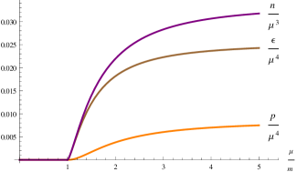
Figure 2: The zeroth-order equilibrium energy density, pressure and charge density as a function of $\mu/m$ at $T=0$ for free massive Dirac fermions. Plots based on eqs. (II.3), (II.3) and (39). $\epsilon$ and $p$ are even functions of $\mu$, whereas $n$ is odd.

The equilibrium charge density is given by the formula $n=\langle J^{0}(\omega=\boldsymbol{k}=0)\rangle^{\prime}$, which implies that for $|\mu|>m$

$$n=\frac{\text{Sign}(\mu)}{3\pi^{2}}\left(\mu^{2}-m^{2}\right)^{3/2},$$ (39)

and $n=0$ for $|\mu|<m$. Clearly, $\epsilon,p$ are even functions of $\mu$, whereas $n$ is odd. Fig. 2 shows plots of $\epsilon,p$ and $n$ for $\mu>0$.

III Thermodynamic Susceptibilities

With the aid of the Kubo formulas discussed in sec. II.2 we can now compute the equilibrium thermodynamic susceptibilities $f_{1},\cdots f_{7}$ for the free massive Dirac field at zero temperature and non-zero chemical potential. The particle number density vanishes for $|\mu|<m$ at $T=0$, as can be seen from the Fermi distribution. Thus for $|\mu|<m$ the system is essentially in its vacuum state. As will become clear from the computations below, all the susceptibilities vanish for $|\mu|<m$.

The Kubo formulas indicate that the susceptibilities can be computed from one-loop diagrams of the form shown in figure 3. Consider for instance the computation of $f_{1}$, given by the Kubo formula eq. (13). We need to first compute the quantity $G_{T^{xy}T^{xy}}$, same as $G_{T^{xy}_{E}T^{xy}_{E}}$, given in terms of the flat space zero-frequency two-point function via

$$\langle T^{xy}(\omega=0,\boldsymbol{k})\,T^{xy}(\omega=0,-\boldsymbol{k})\rangle=(2\pi)^{4}\delta^{4}(0)\,G_{T^{xy}T^{xy}}.$$ (40)

From the expression for the energy-momentum tensor eq. (34) it is straight forward to compute $T^{xy}_{E}(\omega=0,\boldsymbol{k})$, which turns out to be

$$\begin{split}&T^{xy}_{E}(\omega=0,\boldsymbol{k})=\\ &-\frac{i}{4}\int\frac{d^{4}p}{(2\pi)^{4}}\Big{[}\left(\boldsymbol{k}-2\,\boldsymbol{p}\right)_{x}\bar{\Psi}(-p^{0},\boldsymbol{k}-\boldsymbol{p})\,\tilde{\gamma}^{y}\,\Psi(p)\\ &\qquad\qquad\quad+\left(\boldsymbol{k}-2\,\boldsymbol{p}\right)_{y}\bar{\Psi}(-p^{0},\boldsymbol{k}-\boldsymbol{p})\,\tilde{\gamma}^{x}\,\Psi(p)\Big{]},\end{split}$$ (41)

where $p^{\mu}$ is a Euclidean four-vector. Making use of eq. (35) we can now compute $G_{T^{xy}_{E}T^{xy}_{E}}$, which turns out to be

$$G_{T^{xy}_{E}T^{xy}_{E}}=\int\frac{d^{4}q}{(2\pi)^{4}}\Bigg{[}\frac{q_{x}^{2}+q_{y}^{2}}{\big{(}(q^{0}+i\mu)^{2}+\boldsymbol{q}^{2}+m^{2}+k_{z}^{2}-2q_{z}k_{z}\big{)}}-\frac{q_{z}k_{z}(q_{x}^{2}+q_{y}^{2})+8q_{x}^{2}q_{y}^{2}}{\big{(}(q^{0}+i\mu)^{2}+\boldsymbol{q}^{2}+m^{2}\big{)}\big{(}(q^{0}+i\mu)^{2}+\boldsymbol{q}^{2}+m^{2}+k_{z}^{2}-2q_{z}k_{z}\big{)}}\Bigg{]},$$

where, without any loss of generality, we have assumed that $\boldsymbol{k}=(0,0,k_{z})$. Notice that we have shifted $q^{0}\rightarrow q^{0}+i\mu$ to take into account the non-zero value of the chemical potential $\mu$. To compute $f_{1}$ we now act $G_{T^{xy}_{E}T^{xy}_{E}}$ with the operator $\partial^{2}/\partial k_{z}^{2}$ and take the limit $k_{z}\rightarrow 0$. This leaves out the integration over the Euclidean four-vector $q^{\mu}$,

$$\int d^{4}q=\int^{\infty}_{-\infty}dq^{0}\int^{\infty}_{0}dq\,q^{2}\int^{\pi}_{0}d\theta\,\text{sin}\,\theta\int^{2\pi}_{0}d\phi,$$

where we have moved to spherical coordinates for the $\boldsymbol{q}$ integral, with $q\equiv|\boldsymbol{q}|$. The $\theta,\phi$ integrals are easy to perform and can be carried out first. The $q^{0}$ integral can then be performed using contour integration, noting that

$$\begin{split}&\frac{1}{\big{(}(q^{0}+i\mu)^{2}+q^{2}+m^{2}\big{)}^{n}}=\frac{(-1)^{n-1}}{2^{n-1}(n-1)!}\,\times\\ &\quad\underbrace{\frac{1}{m}\frac{\partial}{\partial m}\bigg{(}\frac{1}{m}\frac{\partial}{\partial m}\bigg{(}\cdots}_{n-1\,\text{insertions of}\,\frac{1}{m}\frac{\partial}{\partial m}}\bigg{(}\frac{1}{\big{(}(q^{0}+i\mu)^{2}+q^{2}+m^{2}\big{)}}\bigg{)}\bigg{)}\bigg{)}.\end{split}$$

Thus, whenever the denominator of the integrand for the $q^{0}$ integral involves powers of $\big{(}(q^{0}+i\mu)^{2}+q^{2}+m^{2}\big{)}$ greater than 1, we can rewrite the integrand with appropriate number of derivatives $\frac{1}{m}\frac{\partial}{\partial m}$ extracted out. The left-over $q^{0}$ integrand thus only has simple poles at $q^{0}=-i(\mu\pm\sqrt{q^{2}+m^{2}})$, and the integral can be performed easily. Both the poles for the $q^{0}$ integral lie on the imaginary axis. For $\mu>0$, to have a non-zero contribution we must have $\mu-\sqrt{q^{2}+m^{2}}<0$. On the other hand, for $\mu<0$ we must have $\mu+\sqrt{q^{2}+m^{2}}>0$ to get a non-vanishing result. Both the conditions essentially restrict the domain of integration for $q$ to be $\sqrt{\mu^{2}-m^{2}}\leq q\leq\infty$, along with $|\mu|>m$ for a non-zero result.

We next perform the $q$ integral, which requires a UV cutoff $\Lambda$ to regulate the divergences coming from short distance physics. The cutoff dependence can be removed systematically using the standard renormalization procedure of zero-temperature zero-density quantum field theory. Here we are only interested in $\mu$ dependent terms, which appear independently from cutoff dependent terms. Keeping therefore only the $\mu$ dependent terms and acting upon the result of the $q$ integration with appropriate factors of $\frac{1}{m}\frac{\partial}{\partial m}$ extracted out earlier, we get

$$f_{1}=-\frac{1}{48\pi^{2}}\left[|\mu|\sqrt{\mu^{2}-m^{2}}-m^{2}\log\left(\frac{|\mu|+\sqrt{\mu^{2}-m^{2}}}{m}\right)\right]$$ (42)

for $|\mu|>m$, and $f_{1}=0$ for $|\mu|<m$. Similar computations using the Kubo formulae eqs. (14), (15) and eqs. (19) - (22) give the remaining second order susceptibilities for $|\mu|>m$ to be

$$f_{2}=\frac{|\mu|}{24\pi^{2}}\frac{2m^{2}-3\mu^{2}}{\sqrt{\mu^{2}-m^{2}}},$$ (43)

$$f_{3}=-\frac{|\mu|}{96\pi^{2}}\sqrt{\mu^{2}-m^{2}},$$ (44)

$$f_{4}=\frac{1}{12\pi^{2}}\log\left(\frac{|\mu|+\sqrt{\mu^{2}-m^{2}}}{m}\right),$$ (45)

$$f_{5}=\frac{\text{Sign}(\mu)}{24\pi^{2}}\sqrt{\mu^{2}-m^{2}},$$ (46)

$$f_{6}=-\frac{1}{24\pi^{2}}\left[\frac{|\mu|}{\sqrt{\mu^{2}-m^{2}}}+2\log\left(\frac{|\mu|+\sqrt{\mu^{2}-m^{2}}}{m}\right)\right],$$ (47)

$$f_{7}=\frac{\text{Sign}(\mu)}{12\pi^{2}}\,\frac{3\mu^{2}-2m^{2}}{\sqrt{\mu^{2}-m^{2}}}.$$ (48)

Like $f_{1}$, the susceptibilities $f_{2},\cdots f_{7}$ vanish for $|\mu|<m$. Eqs. (42) - (48) are some of the main results of this paper. Note that $f_{1},\cdots f_{4}$ and $f_{6}$ are even under charge conjugation $\mu\rightarrow-\mu$, whereas $f_{5},f_{7}$ are odd.

Figure 3: The one-loop diagram contributing to the susceptibilities. The nodes correspond to stress tensor and current insertions, depending upon the susceptibility being computed. $k$ denotes the external momentum, while $q$ is the momentum running in the loop.

An interesting limit to consider for the above results is the conformal limit, $m\rightarrow 0$. In the conformal limit, the generating functional eq. (9) has to be invariant under a Weyl rescaling $g_{\mu\nu}\rightarrow\tilde{g}_{\mu\nu}=e^{-2\xi}g_{\mu\nu}$ of the background metric to ensure the tracelessness of the energy-momentum tensor. A quantity $\chi$ that transforms under the above Weyl rescaling as $\chi\rightarrow\tilde{\chi}=e^{w\xi}\chi$ is said to have a Weyl weight $w$. Clearly the measure in eq. (9) has $w=-4$, as $\sqrt{-g}\rightarrow e^{-4\xi}\sqrt{-g}$ under the Weyl rescaling. Thus, for the Weyl invariance of the generating functional eq. (9), each of the terms $f_{n}s_{n}^{(2)}$ must have a Weyl weight of 4. The chemical potential $\mu$ and the temperature $T$, defined through eq. (1), each have $w=1$. The parity even quantities $\Omega^{2}$ and $B\cdot\Omega$ have well defined Weyl weights of $w=2,3$ respectively. In the conformal limit, the Weyl weights of $f_{3}$ and $f_{5}$ from eqs. (44) and (46) are $w=2,1$ respectively, ensuring that the contribution of these two terms to the generating functional is Weyl invariant.

The parity even terms $R,a^{2}$ and $E\cdot a$ do not have well defined Weyl weights. However, the combination

$$\int d^{4}x\sqrt{-g}\left(f\big{(}R+6a^{2}\big{)}-6\,\frac{\partial f}{\partial\mu}E\cdot a\right)$$

is Weyl invariant at $T=0$ for $f=C\mu^{2}$, where $C$ is a constant. Thus, for the Weyl invariance of the generating functional we expect that in the conformal limit $f_{1}=C\mu^{2},f_{2}=6f_{1}$ and $f_{7}=-\,6\,\partial f_{1}/\partial\mu$. From eqs. (42), (43) and (48) we see that in the conformal limit $m\rightarrow 0$ we have $f_{1}=-\mu^{2}/48\pi^{2},f_{2}=-\mu^{2}/8\pi^{2}$ and $f_{7}=\mu/4\pi^{2}$, thereby satisfying the criteria for Weyl invariance, with $C=-1/48\pi^{2}$.

Interestingly, when a conformal field theory is coupled to a background metric and/or a background gauge field, the quantum corrections destroy the tracelessness of the theory. The ensuing trace anomaly is given by Duff (1994); Eling et al. (2013)

$$\begin{split}g_{\mu\nu}T^{\mu\nu}&=-\frac{a}{16\pi^{2}}\left(R_{\mu\nu\alpha\beta}^{2}-4R_{\mu\nu}^{2}+R^{2}\right)\\ &+\frac{c}{16\pi^{2}}\left(R_{\mu\nu\alpha\beta}^{2}-2R_{\mu\nu}^{2}+{\textstyle{\frac{1}{3}}}R^{2}\right)-\frac{b_{0}}{4}F_{\mu\nu}^{2}.\end{split}$$ (49)

Here $a,c$ are numbers that depend upon the field content of the theory; for the theory of free massless Dirac fermions we have $a=11/360,c=1/20$. However, as the terms multiplying $a,c$ in the trace anomaly eq. (49) are fourth order in derivatives, they are not relevant for our present discussion as we are working only upto the second order. The last term in eq. (49) is however second order in derivatives, and must be encoded in the generating functional. Here $b_{0}$ is the coefficient of the one loop $\beta$-function of the coupling $e$ used to minimally couple the theory to external electromagnetic fields,

$$M\frac{d}{dM}\left(\frac{1}{e^{2}}\right)=-\,b_{0}+\mathcal{O}(e^{2}),$$

where $M$ is the renormalization scale, and the action for the external gauge fields is $-\frac{1}{4e^{2}}\int F_{\mu\nu}^{2}$. For a Dirac fermion we have $b_{0}=1/6\pi^{2}$.

Consider now the terms proportional to $E^{2},B^{2}$ in the generating functional, $\int d^{4}x\sqrt{-g}\left(f_{4}B^{2}+f_{6}E^{2}\right)$, which on variation with respect to the metric give the following contribution to the trace of the energy-momentum tensor,

$$g_{\mu\nu}T^{\mu\nu}_{f_{4},f_{6}}=-\left(f^{\prime}_{4}B^{2}+f^{\prime}_{6}E^{2}\right),$$ (50)

where $f^{\prime}_{n}=\mu\,\partial_{\mu}f_{n}+T\,\partial_{T}f_{n}$. From eq. (49) this should be equal to $-\frac{1}{24\pi^{2}}F_{\mu\nu}^{2}=\frac{1}{12\pi^{2}}(E^{2}-B^{2})$, which implies that we should have

$$f^{\prime}_{4}=1/12\pi^{2}\,,\quad f^{\prime}_{6}=-1/12\pi^{2}.$$ (51)

This is indeed borne out by our results in eqs. (45) and (47). Thus the susceptibilities are well behaved in the conformal limit, including the contribution to the trace anomaly.

IV Discussion

We have computed the seven parity even equilibrium thermodynamic susceptibilities appearing at the second order in the hydrodynamic derivative expansion for a free massive Dirac field at zero-temperature and non-zero chemical potential. The resulting susceptibilities, eqs. (42) - (48), can be inserted back into eqs. (11) and (23) to derive the constitutive relations for the Dirac field on a curved background. For the energy-momentum tensor the constitutive relations, with $\lambda\equiv\mu/m>1$, are

$$\mathcal{E}=\epsilon-\frac{m^{2}}{48\pi^{2}}\left(\lambda\sqrt{\lambda^{2}-1}+\log\left(\lambda+\sqrt{\lambda^{2}-1}\right)\right)R+\frac{m^{2}}{24\pi^{2}}\frac{\lambda^{3}(3\lambda^{2}-4)}{(\lambda^{2}-1)^{3/2}}\,a^{2}+\frac{m^{2}}{32\pi^{2}}\frac{\lambda(3\lambda^{2}-2)}{\sqrt{\lambda^{2}-1}}\,\Omega^{2}$$

$$\hskip 219.08621pt+\frac{m^{2}}{24\pi^{2}}\left(\frac{\lambda(1-3\lambda^{2})}{\sqrt{\lambda^{2}-1}}-\log\left(\lambda+\sqrt{\lambda^{2}-1}\right)\right)u^{\alpha}R_{\alpha\beta}u^{\beta},$$ (52a)

$$\mathcal{P}=p-\frac{m^{2}}{144\pi^{2}}\left(\lambda\sqrt{\lambda^{2}-1}-\log\left(\lambda+\sqrt{\lambda^{2}-1}\right)\right)R+\frac{m^{2}}{24\pi^{2}}\frac{\lambda^{3}}{\sqrt{\lambda^{2}-1}}\,a^{2}+\frac{m^{2}}{32\pi^{2}}\lambda\sqrt{\lambda^{2}-1}\,\Omega^{2}$$

$$\hskip 219.08621pt-\frac{m^{2}}{72\pi^{2}}\left(3\lambda\sqrt{\lambda^{2}-1}+\log\left(\lambda+\sqrt{\lambda^{2}-1}\right)\right)u^{\alpha}R_{\alpha\beta}u^{\beta},$$ (52b)

$$\mathcal{Q}_{\mu}=-\frac{m^{2}}{48\pi^{2}}\frac{\lambda(4\lambda^{2}-3)}{\sqrt{\lambda^{2}-1}}\,\epsilon_{\mu\nu\alpha\beta}a^{\nu}u^{\alpha}\Omega^{\beta}-\frac{m^{2}}{24\pi^{2}}\left(2\lambda\sqrt{\lambda^{2}-1}-\log\left(\lambda+\sqrt{\lambda^{2}-1}\right)\right)\,\Delta_{\mu}^{\,\nu}R_{\nu\sigma}u^{\sigma},$$ (52c)

$$\tau_{\mu\nu}=-\frac{m^{2}}{12\pi^{2}}\,\lambda\sqrt{\lambda^{2}-1}\,u^{\alpha}R_{\alpha\langle\mu\nu\rangle\beta}u^{\beta}+\frac{m^{2}}{24\pi^{2}}\left(\lambda\sqrt{\lambda^{2}-1}-\log\left(\lambda+\sqrt{\lambda^{2}-1}\right)\right)R_{\langle\mu\nu\rangle}.$$ (52d)

Here $\epsilon,p$ are zeroth-order energy density and pressure, eqs. (II.3) and (II.3). The constitutive relations for the current are

$$\mathcal{N}=n-\frac{m}{24\pi^{2}}\sqrt{\lambda^{2}-1}\,R+\frac{m}{24\pi^{2}}\frac{6\lambda^{4}-9\lambda^{2}+2}{(\lambda^{2}-1)^{3/2}}\,a^{2}$$

$$\quad+\frac{m}{32\pi^{2}}\frac{2\lambda^{2}-1}{\sqrt{\lambda^{2}-1}}\,\Omega^{2}+\frac{m}{12\pi^{2}}\frac{(2-3\lambda^{2})}{\sqrt{\lambda^{2}-1}}\,u^{\alpha}R_{\alpha\beta}u^{\beta},$$ (53a)

$$\mathcal{J}^{\mu}=-\frac{m}{24\pi^{2}}\frac{2\lambda^{2}-1}{\sqrt{\lambda^{2}-1}}\,\epsilon^{\mu\nu\alpha\beta}u_{\nu}a_{\alpha}\Omega_{\beta}$$

$$\hskip 85.35826pt+\frac{m}{12\pi^{2}}\sqrt{\lambda^{2}-1}\,\Delta^{\mu\nu}R_{\nu\sigma}u^{\sigma},$$ (53b)

with $n$ denoting the zeroth-order charge density, eq. (39). The coefficients of the two-derivative terms appearing in the constitutive relations above are the transport coefficients of the theory.

The susceptibilities $f_{2},f_{6}$ and $f_{7}$ diverge when the magnitude of the chemical potential approaches $m$ from above, i.e. in the limit $|\mu|\rightarrow m^{+}$. This behaviour is carried on to some of the transport coefficients appearing in the constitutive relations eqs. (52) and (53). As discussed in appendix A, the apparent discontinuity across $|\mu|/m=1$ is a consequence of working strictly at zero temperature. At non-zero temperatures the susceptibilities are continuous functions of $\mu/m$.

Second order thermodynamic susceptibilities for a free Dirac field were also computed in Megias and Valle (2014). However, the results are for a massless field at finite temperature, rather than the massive case we have considered. Ref. Buzzegoli et al. (2017) computes the second order constitutive relations using equilibrium three-point functions, which are considerably harder to compute as opposed to the two-point functions we have used. As already mentioned, in equilibrium, the susceptibilities appearing in the generating functional are more fundamental than the transport coefficients in the constitutive relations, which are linear functions of the susceptibilities and their derivatives. Thus it is better to evaluate the susceptibilities first and then compute the transport coefficients from them, a route we have chosen. Besides this, the constitutive relations eqs. (52) and (53) exhibit explicit dependence on the background curvature, something not shown in Buzzegoli et al. (2017).

It would be interesting to make use of the thermodynamic susceptibilities computed here in a physical situation where second order derivative corrections may become relevant. Ref. Kovtun and Shukla (2019) for instance discusses the situation where a non-zero value for the susceptibilities can lead to a shift in the effective Newton’s constant in the presence of matter.

Appendix A Effects of non-zero temperature

In this paper, we have computed parity-even second order equilibrium thermodynamic susceptibilities for a massive Dirac field at zero temperature, eqs. (42)-(48). It seems from the results that the susceptibilities $f_{2},f_{6}$ and $f_{7}$ have a divergent discontinuity across $|\mu|/m=1$, figure 4. However, as we argue below, this discontinuity is an artifact of strictly imposing the $T\rightarrow 0$ limit. At any non-zero value of the temperature the susceptibilities are continuous and well-behaved.

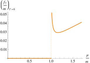
Figure 4: Plot of $f_{7}$ as a function of $\mu/m$ for $\mu>0$ at zero temperature, eq. (48). There is a divergent discontinuity at $\mu/m=1$. Similar discontinuities also exist for $f_{2}$ and $f_{6}$, eqs. (43) and (47).

To illustrate the point, let us consider the computation of $f_{7}$ at a non-zero temperature. The Kubo formula for $f_{7}$ is given by eq. (22). Using the expressions for the energy-momentum tensor and the current presented in section II.3, the zero temperature expression for $f_{7}$ turns out to be

$$\begin{split}&f_{7}^{T=0}=-\frac{1}{2}\lim_{\boldsymbol{k}\to 0}\frac{\partial^{2}}{\partial k_{z}^{2}}\int\frac{d^{4}q}{(2\pi)^{4}}\\ &\quad\frac{4i\tilde{q}_{0}\left(-\tilde{q}_{0}^{2}+\boldsymbol{q}^{2}+m^{2}-k_{z}q_{z}\right)+8i\tilde{q}_{0}q_{x}^{2}}{\left(\tilde{q}_{0}^{2}+\boldsymbol{q}^{2}+m^{2}\right)\left(\tilde{q}_{0}^{2}+\boldsymbol{q}^{2}+m^{2}+k_{z}^{2}-2k_{z}q_{z}\right)},\end{split}$$ (54)

where $\tilde{q}_{0}$ is the shorthand for $q_{0}+i\mu$. When $T\neq 0$, the continuous integral over $q_{0}$ in the expression above has to be replaced by a discrete Matsubara sum,

$$q_{0}\rightarrow\omega_{n}=\frac{(2n+1)\pi}{\beta},\quad\int^{\infty}_{-\infty}\frac{dq_{0}}{2\pi}\rightarrow\frac{1}{\beta}\sum^{\infty}_{n=-\infty},$$

where $\beta\equiv 1/T$ is the inverse temperature. Inserting the above in eq. (54), performing the derivatives and integrating over the angular coordinates in $\boldsymbol{q}$-space gives

$$f_{7}^{T\neq 0}=\frac{1}{15\pi^{2}\beta}\int^{\infty}_{0}dq\,q^{2}\sum^{\infty}_{n=-\infty}\frac{g(z)}{\left(z^{2}-q^{2}-m^{2}\right)^{4}}$$ (55)

with

$$g(z)=2z\left(7q^{4}+10q^{2}\left(3m^{2}-4z^{2}\right)+15\left(m^{4}-z^{4}\right)\right),$$

where $q\equiv|\boldsymbol{q}|$ as before, and $z=i\omega_{n}-\mu$.

Figure 5: The contour $\mathcal{C}$ on the complex $z$ plane alluded to in eq.(56). The dots denote the points $z=i\omega_{n}-\mu$ for $n\in\mathbb{Z}$.

The next step in the evaluation of $f_{7}$ at non-zero temperatures involves evaluating the Matsubara sum in eq. (55). This can be done by converting the sum into a contour integral Kapusta and Gale (2011); Bellac (2011). Consider the function $\frac{\beta}{2}\,\text{tanh}\left(\frac{\beta(z+\mu)}{2}\right)$. This function has poles at $z=i\omega_{n}-\mu$, each with a unit residue, and is otherwise well behaved on the entire complex plane, including being bounded for the limit $z\rightarrow\infty$. This allows us to write the infinite sum in eq. (55) as a contour integral,

$$\begin{split}\mathcal{S}&=\sum^{\infty}_{n=-\infty}\frac{g(z)}{\left(z^{2}-q^{2}-m^{2}\right)^{4}}\\ &=\int_{\mathcal{C}}\frac{dz}{2\pi i}\,\frac{g(z)}{\left(z^{2}-q^{2}-m^{2}\right)^{4}}\,\frac{\beta}{2}\,\text{tanh}\left(\frac{\beta(z+\mu)}{2}\right),\end{split}$$ (56)

where the contour $\mathcal{C}$ is shown in figure 5. This contour can be continuously deformed into the contour $\mathcal{C}_{1}\cup\mathcal{C}_{2}$, figure 6. Now, due to the fact that the integrand in eq. (56) falls off faster than $1/z$ for $z\rightarrow\infty$, we can close $\mathcal{C}_{1}$ with a semicircle $\mathcal{C}_{1}^{\prime}$ to its right and $\mathcal{C}_{2}$ with a semicircle $\mathcal{C}_{2}^{\prime}$ to its left, without affecting the value of $\mathcal{S}$. From the residue theorem it is then clear that the contributions to $\mathcal{S}$ will only come from the poles at $z=\pm\sqrt{q^{2}+m^{2}}\equiv z_{\pm}$, given by

$$\mathcal{S}=-\sum_{z=z_{\pm}}\text{Res}\left[\frac{g(z)}{\left(z^{2}-q^{2}-m^{2}\right)^{4}}\,\frac{\beta}{2}\,\text{tanh}\left(\frac{\beta(z+\mu)}{2}\right)\right],$$ (57)

with the minus sign coming because we have closed the contours in a clockwise manner.

Figure 6: The contour $\mathcal{C}_{1}\cup\mathcal{C}_{2}$. The separation $2\epsilon$ between $\mathcal{C}_{1}$ and $\mathcal{C}_{2}$ tends to zero. $\mathcal{C}_{1}^{\prime}$ and $\mathcal{C}_{2}^{\prime}$ are oriented semicircular arcs of $\infty$ radius which are used to close the contours $\mathcal{C}_{1}$ and $\mathcal{C}_{2}$, respectively.

The result in eq. (57) above can be further simplified by noting that

$$\text{tanh}\left(\frac{\beta(z+\mu)}{2}\right)=1-2\,\mathcal{F}_{-\mu}(z),$$

where $\mathcal{F}_{\mu}(z)=1/\left(e^{\beta(z-\mu)}+1\right)$ is the Fermi-Dirac distribution function. Inserting this in eq. (57) gives

$$\begin{split}\mathcal{S}=&-\frac{\beta}{2}\sum_{z=z_{\pm}}\text{Res}\left[\frac{g(z)}{\left(z^{2}-q^{2}-m^{2}\right)^{4}}\right]\\ &+\beta\sum_{z=z_{\pm}}\text{Res}\left[\frac{g(z)\,\mathcal{F}_{-\mu}(z)}{\left(z^{2}-q^{2}-m^{2}\right)^{4}}\right].\end{split}$$ (58)

The first term in the expression above vanishes, leaving behind the second term, which when substituted into eq. (55) gives

$$f_{7}^{T\neq 0}=\frac{1}{15\pi^{2}}\int^{\infty}_{0}dq\,q^{2}\sum_{z=z_{\pm}}\text{Res}\left[\frac{g(z)\,\mathcal{F}_{-\mu}(z)}{\left(z^{2}-q^{2}-m^{2}\right)^{4}}\right].$$ (59)

Although the residues in eq. (59) above can be readily computed, the leftover integration on $q$ is difficult to perform. The resulting integrand however is a well-behaved function of $q$, and for the sake of illustration, can be integrated numerically for different choices of the temperature $T$. The resulting behaviour of $f_{7}$ as a function of $\mu/m$ is plotted in figure 7 for $\mu>0$ and different choices of the temperature. As is evident from the figure, the smaller the temperature, the stronger the jump in $f_{7}$ around $\mu/m=1$, with the limiting case occurring at $T=0$ as shown in figure 4.

The apparent discontinuities in $f_{2}$ and $f_{6}$ also smoothen out once one deviates from the strict zero temperature condition, just like the case for $f_{7}$. One has to be careful while performing the numerical integration step to obtain the plots for $f_{2}$ and $f_{6}$ at a non-zero temperature due to UV divergences, which have to be carefully subtracted off by adding the appropriate counter terms. The results for $f_{2}$ and $f_{6}$ then are also continuous and well behaved.

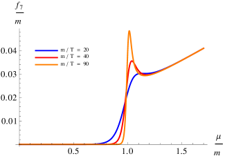
Figure 7: Plots depicting the behaviour of $f_{7}$ as a function of $\mu/m$ for $\mu>0$ at different non-zero temperatures. As the temperature becomes smaller, the jump in $f_{7}$ as well as the peak height around $\mu/m=1$ become more prominent, with the limiting case $T=0$ plotted in figure 4. In an identical manner the non-zero temperature also removes the discontinuity at $\mu=-m$.

References

• Kovtun and Shukla (2018) Pavel Kovtun and Ashish Shukla, “Kubo formulas for thermodynamic transport coefficients,” JHEP 10, 007 (2018)arXiv:1806.05774 [hep-th] .
• Landau and Lifshitz (2013) L.D. Landau and E.M. Lifshitz, Fluid Mechanics, v. 6 (Elsevier Science, 2013).
• Kovtun (2012) Pavel Kovtun, “Lectures on hydrodynamic fluctuations in relativistic theories,” INT Summer School on Applications of String Theory Seattle, Washington, USA, July 18-29, 2011J. Phys. A45, 473001 (2012)arXiv:1205.5040 [hep-th] .
• Romatschke and Romatschke (2019) Paul Romatschke and Ulrike Romatschke, “Relativistic Fluid Dynamics In and Out of Equilibrium,”   (2019), arXiv:1712.05815 [nucl-th] .
• Baier et al. (2008) Rudolf Baier, Paul Romatschke, Dam Thanh Son, Andrei O. Starinets,  and Mikhail A. Stephanov, “Relativistic viscous hydrodynamics, conformal invariance, and holography,” JHEP 04, 100 (2008)arXiv:0712.2451 [hep-th] .
• Bhattacharyya et al. (2008) Sayantani Bhattacharyya, Veronika E Hubeny, Shiraz Minwalla,  and Mukund Rangamani, “Nonlinear Fluid Dynamics from Gravity,” JHEP 02, 045 (2008)arXiv:0712.2456 [hep-th] .
• Jensen et al. (2012a) Kristan Jensen, Matthias Kaminski, Pavel Kovtun, Rene Meyer, Adam Ritz,  and Amos Yarom, “Parity-Violating Hydrodynamics in 2+1 Dimensions,” JHEP 05, 102 (2012a)arXiv:1112.4498 [hep-th] .
• Banerjee et al. (2012) Nabamita Banerjee, Jyotirmoy Bhattacharya, Sayantani Bhattacharyya, Sachin Jain, Shiraz Minwalla,  and Tarun Sharma, “Constraints on Fluid Dynamics from Equilibrium Partition Functions,” JHEP 09, 046 (2012)arXiv:1203.3544 [hep-th] .
• Jensen et al. (2012b) Kristan Jensen, Matthias Kaminski, Pavel Kovtun, Rene Meyer, Adam Ritz,  and Amos Yarom, “Towards hydrodynamics without an entropy current,” Phys. Rev. Lett. 109, 101601 (2012b)arXiv:1203.3556 [hep-th] .
• Shapiro and Teukolsky (1983) S. L. Shapiro and S. A. Teukolsky, Black holes, white dwarfs, and neutron stars: The physics of compact objects (1983).
• Glendenning (1997) N. K. Glendenning, Compact stars: Nuclear physics, particle physics, and general relativity (1997).
• Vuorinen (2019) Aleksi Vuorinen, “Neutron stars and stellar mergers as a laboratory for dense QCD matter,” Proceedings, 27th International Conference on Ultrarelativistic Nucleus-Nucleus Collisions (Quark Matter 2018): Venice, Italy, May 14-19, 2018Nucl. Phys. A982, 36–42 (2019)arXiv:1807.04480 [nucl-th] .
• Annala et al. (2019) Eemeli Annala, Tyler Gorda, Aleksi Kurkela, Joonas Nättilä,  and Aleksi Vuorinen, “Constraining the properties of neutron-star matter with observations,” in 12th INTEGRAL conference and 1st AHEAD Gamma-ray workshop (INTEGRAL 2019): INTEGRAL looks AHEAD to Multi-Messenger Astrophysics Geneva, Switzerland, February 11-15, 2019 (2019) arXiv:1904.01354 [astro-ph.HE] .
• Alford et al. (2008) Mark G. Alford, Andreas Schmitt, Krishna Rajagopal,  and Thomas Schäfer, “Color superconductivity in dense quark matter,” Rev. Mod. Phys. 80, 1455–1515 (2008)arXiv:0709.4635 [hep-ph] .
• Kurkela et al. (2010) Aleksi Kurkela, Paul Romatschke,  and Aleksi Vuorinen, “Cold Quark Matter,” Phys. Rev. D81, 105021 (2010)arXiv:0912.1856 [hep-ph] .
• Ghisoiu et al. (2017) Ioan Ghisoiu, Tyler Gorda, Aleksi Kurkela, Paul Romatschke, Matias Säppi,  and Aleksi Vuorinen, “On high-order perturbative calculations at finite density,” Nucl. Phys. B915, 102–118 (2017)arXiv:1609.04339 [hep-ph] .
• Kovtun (2016) Pavel Kovtun, “Thermodynamics of polarized relativistic matter,” JHEP 07, 028 (2016)arXiv:1606.01226 [hep-th] .
• Hernandez and Kovtun (2017) Juan Hernandez and Pavel Kovtun, “Relativistic magnetohydrodynamics,” JHEP 05, 001 (2017)arXiv:1703.08757 [hep-th] .
• Moore and Sohrabi (2011) Guy D. Moore and Kiyoumars A. Sohrabi, “Kubo Formulae for Second-Order Hydrodynamic Coefficients,” Phys. Rev. Lett. 106, 122302 (2011)arXiv:1007.5333 [hep-ph] .
• Moore and Sohrabi (2012) Guy D. Moore and Kiyoumars A. Sohrabi, “Thermodynamical second-order hydrodynamic coefficients,” JHEP 11, 148 (2012)arXiv:1210.3340 [hep-ph] .
• DeWitt (2003) B.S. DeWitt, The Global Approach to Quantum Field Theory Vol. 1, International series of monographs on physics, Vol. 114 (Clarendon Press, 2003).
• Buzzegoli and Becattini (2018) M. Buzzegoli and F. Becattini, “General thermodynamic equilibrium with axial chemical potential for the free Dirac field,” JHEP 12, 002 (2018)arXiv:1807.02071 [hep-th] .
• Duff (1994) M. J. Duff, “Twenty years of the Weyl anomaly,” Conference on Highlights of Particle and Condensed Matter Physics (SALAMFEST) Trieste, Italy, March 8-12, 1993Class. Quant. Grav. 11, 1387–1404 (1994)arXiv:hep-th/9308075 [hep-th] .
• Eling et al. (2013) Christopher Eling, Yaron Oz, Stefan Theisen,  and Shimon Yankielowicz, “Conformal Anomalies in Hydrodynamics,” JHEP 05, 037 (2013)arXiv:1301.3170 [hep-th] .
• Fuini and Yaffe (2015) John F. Fuini and Laurence G. Yaffe, “Far-from-equilibrium dynamics of a strongly coupled non-Abelian plasma with non-zero charge density or external magnetic field,” JHEP 07, 116 (2015)arXiv:1503.07148 [hep-th] .
• Megias and Valle (2014) Eugenio Megias and Manuel Valle, “Second-order partition function of a non-interacting chiral fluid in 3+1 dimensions,” JHEP 11, 005 (2014)arXiv:1408.0165 [hep-th] .
• Buzzegoli et al. (2017) M. Buzzegoli, E. Grossi,  and F. Becattini, “General equilibrium second-order hydrodynamic coefficients for free quantum fields,” JHEP 10, 091 (2017), [Erratum: JHEP07,119(2018)], arXiv:1704.02808 [hep-th] .
• Kovtun and Shukla (2019) Pavel Kovtun and Ashish Shukla, “Einstein’s Equations in Matter,”   (2019), arXiv:1907.04976 [gr-qc] .
• Kapusta and Gale (2011) J. I. Kapusta and Charles Gale, Finite-temperature field theory: Principles and applications, Cambridge Monographs on Mathematical Physics (Cambridge University Press, 2011).
• Bellac (2011) Michel Le Bellac, Thermal Field Theory, Cambridge Monographs on Mathematical Physics (Cambridge University Press, 2011).