Abstract

The calibration procedures for data collected for Argus and the 4mm Receiver instruments on the GBT are presented. The measured beam size, aperture efficiency, and main-beam efficiency are derived for the range of observing frequencies (66–116 GHz) within the 3 mm atmospheric window. The telescope performs well even at the highest frequencies ($>$100 GHz). The amount of power in the error pattern of the antenna beam is estimated. Approximately 95% of the total antenna power is contained within $1^{\circ}$ of the pointed direction. The calibration derived using small sources follows theoretical expectations based on the Ruze equation. In general, bright point source calibrators that are monitored regularly by ALMA can be used to accurately derive the main-beam efficiency of the telescope.

1 Introduction

The 4mm Receiver (Rcvr68_92) and Argus (RcvrArray75_115) were commissioned on the Robert C. Byrd Green Bank Telescope (GBT) in 2012 and 2016 respectively. The results from commissioning, measured instrument performance, and calibration summaries are given on the instrument web pages. A short test project was carried out in 2018 April to verify the relative calibration of the 4mm Receiver and Argus. Using these data and the archival calibration data from science programs, the calibration results for Argus and the 4mm Receiver are presented in this memo. The calibration of GBT at lower observing frequencies, which is based on noise-diodes, is discussed in the GBTIDL spectral-line processing documentation Braatz (2009).

The table of observations used in this memo is provided in Appendix A, and the telescope efficiencies are defined in their integral forms in Appendix B.

2 Temperature Scales and Efficiency Definitions

The antenna temperature ($T_{A}$) is related to antenna temperature corrected for atmosphere ($T_{A}^{\prime}$) by

$$T_{A}^{\prime}=T_{A}\,\exp(\tau_{o}\,A),$$ (1)

where $\tau_{o}$ is the zenith opacity and $A$ is the airmass which can be approximated by $A\simeq 1.0/\sin({\rm El})$, except at very low elevations (El).

The forward beam brightness temperature $T_{A}^{*}$ is the effective beam brightness temperature seeing the entire the sky corrected for atmosphere.

$$T_{A}^{*}=\frac{T_{A}^{\prime}}{\eta_{l}},$$ (2)

where $\eta_{l}$ represents the faction of power in the forward $2\pi$ steradian direction on the sky and ($1-\eta_{l}$) is the rear “spillover” and scattering fraction that sees the ground. Following the convention of Kutner & Ulich (1981), the value $\eta_{l}$ is a combination of the radiation efficiency $\eta_{r}$ that corrects for ohmic losses and the “rearward” scattering and spillover efficiency ($\eta_{rss}$), where $\eta_{l}=\eta_{r}\,\eta_{rss}$. Since $\eta_{r}\simeq 1.0$ for radio telescopes, $\eta_{l}\simeq\eta_{rss}$. Using the definitions adopted for the IRAM 30m (Kramer 1997), $\eta_{l}$ is the forward efficiency (F_eff). For the unblocked aperture, the feed-arm design, and Gregorian geometry of the GBT, the forward efficiency is expected to be approximately $\eta_{l}\simeq 0.99$ (Srikanth 1989a,b).

The main-beam efficiency $(\eta_{mb})$ is used to relate $T_{A}^{\prime}$ to the measured main-beam antenna temperature ($T_{mb}$) by

$$T_{mb}=\frac{T_{A}^{\prime}}{\eta_{mb}}.$$ (3)

The main-beam efficiency represents the fraction of power contained within the main-beam lobe of the antenna pattern.

Kutner & Ulich (1981) introduced $T_{R}^{*}$ which corrects for both forward and rearward losses.

$$T_{R}^{*}=\frac{T_{A}^{\prime}}{\eta_{l}\,\eta_{fss}},$$ (4)

where $\eta_{fss}$ is called the “forward” scattering and spillover efficiency. The value $\eta_{fss}$ is the faction of power in the forward $2\pi$ direction that is contained within the diffraction pattern of the telescope including the error beam pattern (Appendix B). The corrected main-beam efficiency ($\eta_{M}^{*}$) relates the $T_{R}^{*}$ temperature scale to the main-beam $T_{mb}$ temperature scale (Mangum 1999);

$$\eta_{M}^{*}=\frac{T_{R}^{*}}{T_{mb}}=\frac{\eta_{mb}}{\eta_{l}\,\eta_{fss}}.$$ (5)

Single-dish astronomers typically report observational results using temperature scales of either $T_{A}^{\prime}$, $T_{mb}$, $T_{a}^{*}$, or $T_{R}^{*}$, depending on the calibration practices at individual telescopes and their scientific needs. These temperature scales are not the same, and are related by the following expressions:

$$T_{A}^{\prime}\,=\,\eta_{mb}\,T_{mb}\,=\,\eta_{l}\,T_{A}^{*}\,=\,\eta_{l}\,\eta_{fss}\,T_{R}^{*}.$$ (6)

2.1 Small Sources

For sources much smaller than the telescope beam, the aperture efficiency ($\eta_{a}$) of the telescope relates the flux density ($S_{\nu}$) of the source to $T_{A}^{\prime}$. For the 100m GBT, the aperture efficiency is

$$\eta_{a}=0.352\frac{T_{A}^{\prime}}{S_{\nu}}.$$ (7)

Assuming the Ruze equation, the aperture efficiency is related to the surface errors of the telescope by:

$$\eta_{a}=\eta_{0}\exp[-(4\pi\epsilon/\lambda)^{2})],$$ (8)

where the coefficient $\eta_{0}=0.71$ is the GBT aperture efficiency at long wavelengths, $\epsilon$ is the rms uncertainty of the surface, and $\lambda$ is the observing wavelength. Currently for optimal GBT surface corrections and under excellent observing conditions, $\epsilon\simeq 230$ $\mu$m (Frayer et al. 2018).

Assuming a Gaussian beam and for point sources, the main-beam efficiency is given by

$$\eta_{mb}=0.8899\eta_{a}\left(\theta_{FWHM}\frac{D}{\lambda}\right)^{2},$$ (9)

where $\theta_{FWHM}$ is the full-width half-maximum beam size in radians and D is the 100m diameter of the GBT (Maddalena 2010).

2.2 Extended Sources

For sources much larger than the telescope beam, the source brightness temperature ($T_{S}$) is well approximated by the main-beam temperature, i.e., $T_{mb}\simeq T_{S}$. However, measurements of extended sources includes power on spatial scales that resides outside of the main-beam lobe. The measured antenna temperature depends on the coupling of the source structure with the full the antenna beam pattern, including the error pattern. Defining the efficiency with which the antenna couples to the source as $\eta_{c}$ (Appendix B), $T_{A}^{\prime}=\eta_{c}\eta_{fss}\eta_{l}\,T_{S}$. This definition is consistent with Kutner & Ulich (1981) where $T_{R}^{*}=\eta_{c}\,T_{S}$. The efficiency terms can be combined to define the effective beam efficiency for a source as

$$\eta_{\rm Source}=\eta_{c}\eta_{fss}\eta_{l},$$ (10)

such that for an extended source

$$T_{A}^{\prime}=\eta_{\rm Source}\,T_{S}.$$ (11)

3 Calibration Equations

The equations associated with the calibration of the 4mm Receiver were previously presented in the 67-93.6 GHz Spectral Line Survey paper for Orion-KL (Frayer et al. 2015). The equations for Argus are based on Kutner & Ulich (1981) and are summarized on the Argus web page. The 4mm Receiver has both a cold and ambient load (“two load” system) while Argus only has an ambient load (“one load” system) so the calibration approaches of the two instruments are slightly different. Both approaches are summarized here.

3.1 The 4mm Receiver

The 4mm Receiver has two feeds that are separated by a cold load within the cryostat. A calibration wheel rotates above the cryostat which permits the feeds to see the sky, the ambient load, or mirrors that enable the feeds to look back down into the cryostat at the cold load. Using both loads for the 4mm Receiver, the gain ($g$) is given by

$$g=[(T_{amb}-T_{cold})/(C_{amb}-C_{cold})],$$ (12)

where $T_{amb}$ and $T_{cold}$ are the temperatures of the ambient and cold loads and $C_{amb}$ and $C_{cold}$ are the observed counts of the ambient and cold loads. The temperature of ambient load is measured by a temperature sensor in real-time, while the effective temperature of the cold load has been measured in the lab using an external liquid nitrogen load. At the default frequency of 77 GHz for the Auto observing procedures for the 4mm Receiver, the cold load is estimated to be 54 K. Lab measurements suggest the effective cold load temperature decreases roughly linearly from 60 K at 67 GHz to about 45 K at 92 GHz. The cold load temperature in units of Kelvin is expressed as a function of frequency by

$$T_{cold}=54.0\,{\rm K}-0.6{\rm[K/GHz]}(\nu-77.0\,{\rm GHz}),$$ (13)

where $\nu$ is the observing frequency in units of GHz. By using this relationship, the uncertainty on $T_{cold}$ is estimated to be about 4 K which corresponds to an uncertainty on the gain and the measured $T_{A}$ temperature scale of less than 2%.

For most GBT observations, the (ON$-$OFF)/OFF processing method is adopted. Using this approach, the observed antenna temperature is

$$T_{A}=T_{\rm sys}(C_{ON}-C_{OFF})/C_{OFF},$$ (14)

where $C_{ON}$ and $C_{OFF}$ are the observed counts of the ON and OFF scans. The system temperature ($T_{\rm sys}$) is given by

$$T_{\rm sys}=g\,C_{OFF},$$ (15)

where the gain is given by equation (12). For the default calibration procedures, both $T_{\rm sys}$ and $g$ are scalar values representing the median or average across the central region of the spectral bandpass. The observed antenna temperature is corrected for atmosphere ($T_{A}^{\prime}$) using equation (1). The opacity is derived from the Observatory’s weather database derived for Green Bank. Except for periods of rapidly changing weather conditions, the predicted opacities are accurate to within $\Delta\tau_{o}\simeq 0.01$ based on historical measurements.

3.2 Argus

The Argus instrument is a 16 element focal-plane-array operating from 74 GHz to 116 GHz. It has a chopper-vane absorber that can be placed over the array for calibration. For the chopper-vane technique with only one load, the natural temperature scale measured by the antenna is $T_{A}^{*}$ (Kutner & Ulich 1981; Kramer 1997). This temperature scale has the advantage of being corrected for atmospheric attenuation while its derivation is nearly independent of opacity.

Analogous to equation (12), the “gain” for a one load system is derived from the difference of signals measured between the ambient load and blank sky.

$$g=[(T_{amb}-T_{OFF})/(C_{amb}-C_{OFF})],$$ (16)

where $T_{amb}$ and $T_{OFF}$ are the temperatures of the ambient load and the blank sky (OFF) and $C_{amb}$ and $C_{OFF}$ are the corresponding observed counts of the ambient load and blank sky. The $T_{A}^{*}$ temperature is

$$T_{A}^{*}=T_{cal}(C_{ON}-C_{OFF})/(C_{amb}-C_{OFF}),$$ (17)

where

$$T_{cal}=(T_{amb}-T_{OFF})\exp(\tau_{o}\,A)/\eta_{l}.$$ (18)

The difference $T_{amb}-T_{OFF}$ removes the receiver temperature and other telescope systematics, and is given by

$$(T_{amb}-T_{OFF})=T_{amb}-(\eta_{l}\,T_{sky}+(1-\eta_{l})\,T_{spill})$$ (19)

where $\eta_{l}\,T_{sky}$ is the contribution from the sky and $(1-\eta_{l})\,T_{spill}$ is the contribution from ground spillover. The temperature of the sky is

$$T_{sky}=T_{ATM}(1-\exp(-\tau_{o}\,A))+T_{bg}\exp(-\tau_{o}\,A),$$ (20)

where $T_{ATM}$ is the effective atmospheric temperature and $T_{bg}$ is the cosmic microwave background temperature of 2.73 K. With a little algebra, the equations can be reduced to

$$T_{cal}=(T_{ATM}-T_{bg})+(T_{spill}-T_{ATM})\exp(\tau_{o}\,A)+(T_{amb}-T_{spill})\exp(\tau_{o}\,A)/\eta_{l}.$$ (21)

Equation (21) is the same as equation (8) of Kramer (1997) and equation (12) of Kutner & Ulich (1981). If $T_{amb}\simeq T_{spill}$ or if $\eta_{l}\simeq 1$ (which are both good approximations for the GBT), then

$$T_{cal}\simeq(T_{ATM}-T_{bg})+(T_{amb}-T_{ATM})\exp(\tau_{o}\,A).$$ (22)

Based on the 2017/2018 observing season with Argus on the GBT, the average $T_{cal}/T_{amb}$ ratio using equation (22) is $0.997\pm 0.018$. Hence, one could approximate the calibration by simply assuming

$$T_{cal}\approx T_{amb}.$$ (23)

For example, if one adopts typical values ($T_{bg}=2.7$ K, $\exp(\tau_{o}\,A)=1.2$, $\eta_{l}\simeq 0.99$, $T_{ATM}=260$ K, $T_{spill}=270$ K, $T_{amb}=273$ K), one finds that equations (21, 22, & 23) all yield the same value of $T_{cal}\simeq 273$ K. This approximation works best for average observing conditions. In the coldest conditions $T_{amb}<260$ K, equation (23) tends to overestimate $T_{cal}$ by about 0.7%, and the $T_{cal}\approx T_{amb}$ approximation begins to break down with large atmospheric opacities ($\exp[\tau_{o}\,A]>1.7$) where $T_{cal}$ is underestimated by 5-10%.

For Argus observations, the chopper-vane calibration is done at least every 30-45 minutes which is the recommended time between pointing and focus observations. The measured signal from the vane has been shown to be stable over a time scale of more than one hour in good conditions. However, the effective system temperature can change rapidly with varying sky conditions as a function of time. To correct for the varying effective system temperature and analogous to equation (14),

$$T_{A}^{*}=T_{\rm sys}^{*}(C_{ON}-C_{OFF})/C_{OFF},$$ (24)

where $C_{ON}$ and $C_{OFF}$ are the observed counts of the ON and OFF scans, and the effective system temperature ($T_{\rm sys}^{*}$) as a function of time ($t$) is given by

$$T_{\rm sys}^{*}(t)=T_{cal}/(C_{amb}/C_{OFF}(t)-1).$$ (25)

The effective system temperature is related to $T_{sys}$ by

$$T_{\rm sys}^{*}=T_{sys}\exp(\tau_{o}\,A)/\eta_{l}.$$ (26)

Equations (24) and (25) are used to calibration the raw counts into $T_{A}^{*}$ for the Argus VEGAS (spectrometer) data, with $T_{cal}$ given by equation (22). For the default calibration procedures, $T_{\rm sys}^{*}$ and $T_{cal}$ are scalar values representing the median or average across the central region of the spectral bandpass. For the pointing and focus data taken with the Digital Continuum Receiver (DCR), equation (23) is adopted for $T_{cal}$ when reporting system temperatures within the Astrid observing window.

3.3 Equation Simplifications

For simplicity, the equations in §3 adopt the Rayleigh-Jeans approximation, i.e., $J(T)=T$, where ($h\,\nu<<k\,T$). The physical temperatures should be replaced by the Planck function radiation temperature ($J_{\nu}(T_{b}$)) for accurate calculations. The Planck function radiation temperature is

$$J_{\nu}(T_{b})=\frac{h\,\nu}{k}\left(\exp\left[\frac{h\,\nu}{k\,T_{b}}\right]-1\right)^{-1},$$ (27)

where $T_{b}$ is the brightness temperature.

Another simplification to the standard calibration equations arises since both the 4mm Receiver and Argus are single side-band systems. For single side-band receivers, the signal from the image side-band is negligible such that such that $G_{i}/G_{s}\simeq 0$, for comparison with the equations of Kutner & Ulich (1981) and Kramer (1997).

4 Results

The calibration of Argus and the 4mm Receiver is tied to the ALMA calibration system using the online ALMA Calibrator Source Catalog (https://almascience.eso.org/sc/). This web-tool is used to derive the flux densities of bright 3mm quasars for absolute flux calibration of Argus and the 4mm Receiver. The cataloged ALMA Band-3 measurements at 91.5 GHz and 103.5 GHz are extrapolated to the observed GBT frequency using the inferred Band-3 spectral-index and interpolated in time between ALMA measurements surrounding the GBT observations. ALMA regularly observes all bright 3mm quasars that are visible at the ALMA site (23^∘ South), including even 3C84 which is at a declination of $+41.5^{\circ}$.

In addition to using bright 3mm quasars, observations of Jupiter, Mars, and the Moon were used to measure the beam efficiency associated with different source sizes. The forward efficiency $\eta_{l}$ is estimated to be 0.985, and this value is adopted for this memo. Accurate absolute measurements of $\eta_{l}$ are challenging to measure at 3mm on the GBT due to weather dependencies and since its value is near 1. Based on tipping observations and comparisons between $T_{A}^{*}$ and $T_{A}^{\prime}$, $\eta_{l}\simeq 0.985\pm 0.015$. This is consistent with the theoretical expectations for the GBT of $\eta_{l}\simeq 0.99$ (Srikanth 1989a; Srikanth 1989b). Possible variations of $\eta_{l}$ as a function of elevation are not included in this memo.

4.1 Comparison Between the 4mm Receiver and Argus

Observations were carried out on 2018 April 06 to compare the relative calibration of the 4mm Receiver and Argus (GBT project and session: TGBT17B_502_01). No significant difference in the calibration of these instruments were found using their respective calibration approaches outlined in §3. Observations of the bright quasar 3C279 were used to measure the aperture efficiencies, while observations of Jupiter and the Moon were used to derive the beam efficiencies for these extended sources.

The aperture efficiencies were derived using equation (7). The beam efficiencies associated with extended sources were derived using

$$\eta_{\rm Source}=\frac{T_{A}^{\prime}}{J_{\nu}(T_{b})}=\frac{\eta_{l}T_{A}^{*}}{J_{\nu}(T_{b})}.$$ (28)

Since Jupiter and the Moon are much larger than the beam size, equation (11) is applicable. The brightness temperature ($T_{b}$) as a function of frequency for the planets were taken from the CASA software package (Butler 2012). The radiation temperature of the Moon was computed based on the phase of the Moon at the time of observations using the formulae presented in Mangum (1993).

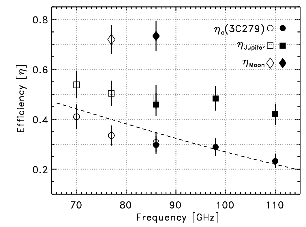
Figure 1: The comparison of calibration measurements made with the W-band 4mm Receiver (open symbols) and Argus (solid symbols) within the same observing session (§4.1). The point-source aperture efficiencies are shown as circles, while the measured beam efficiencies of Jupiter and the Moon are shown as squares and diamonds, respectively. The aperture efficiency based on the average good weather surface error of 235$\mu$m is shown as the dashed-line for comparison.

Figure 1 shows the comparison of the measurements. The values derived for 3C279, Jupiter, and the Moon were all consistent within measurement errors between the 4mm Receiver and Argus. The measured beam efficiency for the Moon is larger than that observed for Jupiter which implies significant power within the beam pattern on spatial scales between $\sim 40^{\prime\prime}$ (size of Jupiter) and $32^{\prime}$ (size of the Moon). The measured efficiencies were not optimal as the weather was somewhat marginal for calibration observations (moderate opacities that varied significantly throughout the observing session). The dashed-line shows the expected aperture efficiency based on an effective surface uncertainty of 235$\mu$m, which is the best-fit average value for quality observations during the 2017 and 2018 observing seasons (§4.2).

4.2 Small Source Calibration

Approximately 200 measurements of point sources were collected using observations with the 4mm Receiver and Argus from 2017 February through 2019 March to quantify the performance of the GBT within the 3 mm atmospheric window (Appendix A). Only observations of the brightest point-source calibrators were used ($S{\nu}>3$ Jy), and sessions with questionable pointing, focus, or surface corrections were discarded. The sample used for this analysis is not complete, but is representative of the wide range of conditions over the full high-frequency observing season (October through April) in Green Bank.

4.2.1 Beam Size

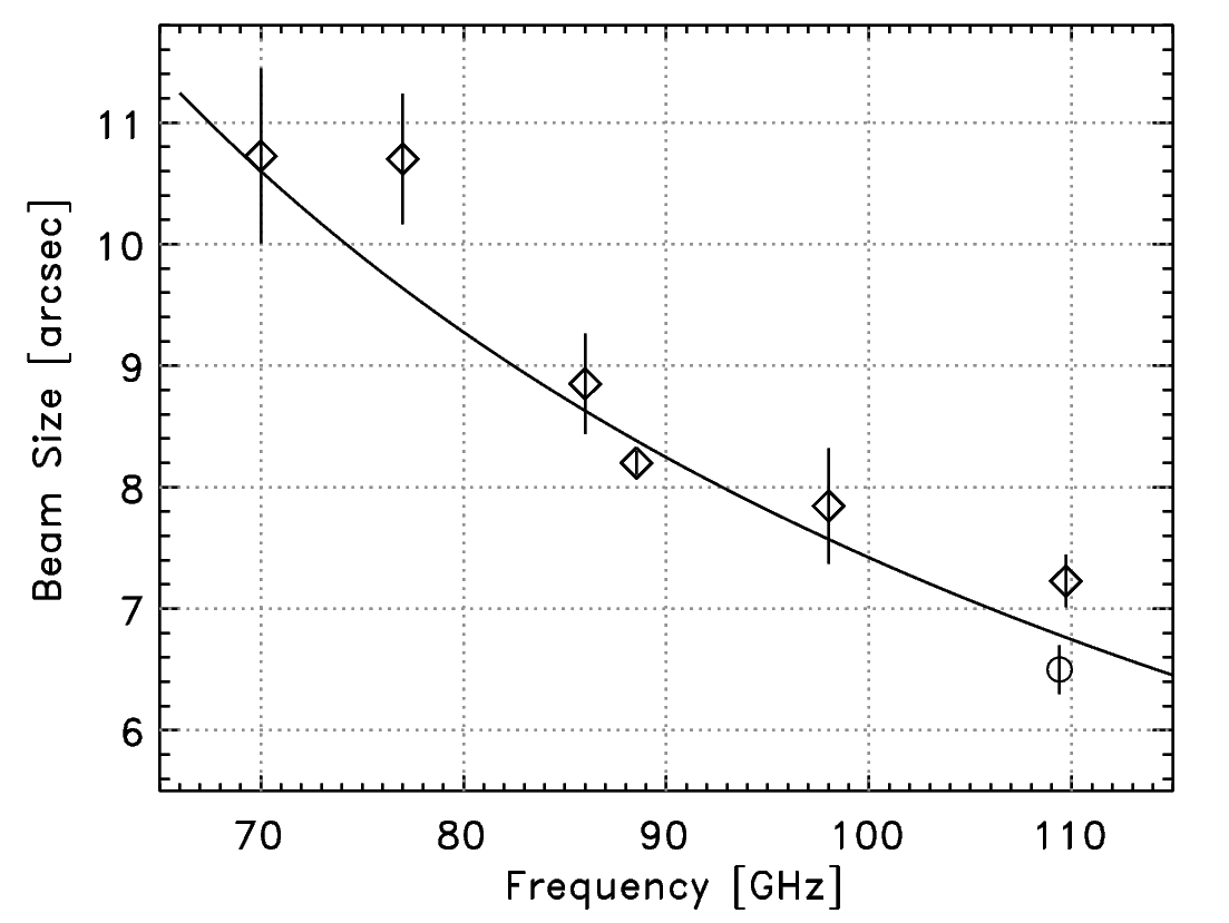
Figure 2: The measured average $\theta_{\rm FWHM}$ beam sizes as a function of frequency shown as diamonds. The solid line corresponds to $1.2\lambda/D$. On average there is some degradation of the measured beam size at highest frequencies ($\nu>100$ GHz), but the open circle shows the result at 109 GHz derived in excellent conditions (GBT Memo#296) for comparison.

Figure 2 shows the measured beam sizes as a function of frequency. The error bars represented the measurement uncertainty of individual measurements divided by the square-root of the number of observations within each frequency bin. Most observations, to date, have been done within the 86–90 GHz frequency band corresponding to HCN(1-0) and HCO⁺(1-0) and that of ¹³CO near 110 GHz. The solid line in Figure 2 corresponds to

$$\kappa\equiv\theta_{\rm FWHM}\left(\frac{D}{\lambda}\right)=1.20,$$ (29)

whose normalization is derived from the best fit parameter of $\kappa=1.20\pm 0.02$ over all frequencies. Under typical conditions, the beam performance degrades slightly at the highest frequencies. This is shown by the data point lying above the line in Figure 2 at frequencies near 110 GHz.

The effective $\kappa$ for individual observing sessions range from about 1.15 to 1.3, depending on the winds and the derived telescope corrections. Under very good conditions, one can achieve $\kappa<1.18$ even at high-frequency. For example, a value of $\kappa=1.16$ was derived at 109.4 GHz in calm conditions and with very low opacity. This result is discussed in GBT Memo#296 (Frayer 2017) and is shown by the open circle in Figure 2.

4.2.2 Aperture and Main-Beam Efficiencies

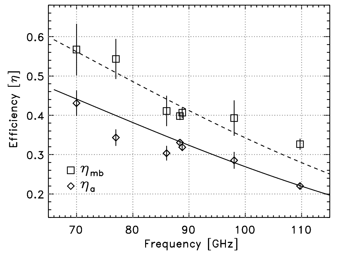
Figure 3: The measured aperture and main-beam efficiencies as a function of frequency. The diamonds represent the aperture efficiencies, while the squares are the measured main-beam efficiencies derived for point sources. The solid line shows the aperture efficiencies predicted by the Ruze equation with an effective surface error of 235$\mu$m. The dashed line corresponds to an average ratio of $\eta_{mb}/\eta_{a}=1.274$.

For the sample of bright point-sources, the aperture efficiencies were derived using equation (7). The results as a function of frequency are consistent with the Ruze equation (equation 8) with an effective surface error of 235$\mu$m. This value represents all losses (e.g., pointing errors, focus errors, tracking errors due to winds and telescope servo system, as well as surface errors from the dish and subreflector). The main-beam efficiency was derived from the measurements of the peak scans of the pointing sources using equation (9). The uncertainties on the individual observations are large due to measurement errors. The typical measurement uncertainties on $\eta_{a}$ and $\theta_{FWHM}$ result in a 23% measurement error on $\eta_{mb}$. The uncertainties plotted in Figure 3 represent the measurement uncertainty of individual observations divided by the square-root of the number of observations within each frequency bin. The data points near 88 GHz and 110 GHz are the most accurate due to the large number of observations made at these frequencies.

From the derived efficiencies and errors within each frequency bin, the weighted average ratio derived is

$$\frac{\eta_{mb}}{\eta_{a}}=1.274\pm 0.035.$$ (30)

This ratio is consistent with the average beam size parameter of $\kappa=1.20$ derived in §4.2.1, assuming a Gaussian beam. The $\eta_{mb}$ data point measured near 110 GHz is higher than would be implied by equation 30, which results from the slightly larger average value of $\kappa$ at this frequency as shown in Figure 2.

4.3 Corrected Main Beam Efficiency

The corrected main-beam efficiency $\eta_{M}^{*}$ can be inferred from observations, but since it depends significantly on the error beam pattern, theoretical considerations are typically used to estimate its value. Using the relationships associated with the Ruze equation (see discussion in Baars 1973 and the application for the NRAO 12m in Mangum 1999),

$$\eta_{M}^{*}=\left(1+\frac{A_{E}\theta_{E}^{2}}{A_{M}\theta_{M}^{2}}\right)^{-1},$$ (31)

where $A$ and $\theta$ are the amplitudes and half-power width, respectively, corresponding to the error ($E$) and main ($M$) beam patterns.

Assuming a Gaussian beam and a Gaussian error pattern, the value $(A_{E}\theta_{E}^{2})/(A_{M}\theta_{M}^{2})$ represents the ratio of power in the error pattern compared to the main beam. The FWHM spatial scale of the error pattern is

$$\theta_{E}=\frac{2}{\pi}\sqrt{\ln(2)}\left(\frac{\lambda}{c_{\sigma}}\right),$$ (32)

where $c_{\sigma}$ is the surface deviation correlation radius. The ratio of the amplitude of the error beam relative to the amplitude of the main beam is given by

$$\frac{A_{E}}{A_{M}}=\frac{1}{\eta_{0}}\left[\frac{2\,c_{\sigma}}{D}\right]^{2}\,(\exp(\delta^{2})-1),$$ (33)

where $\delta=4\pi\,\epsilon/\lambda$.

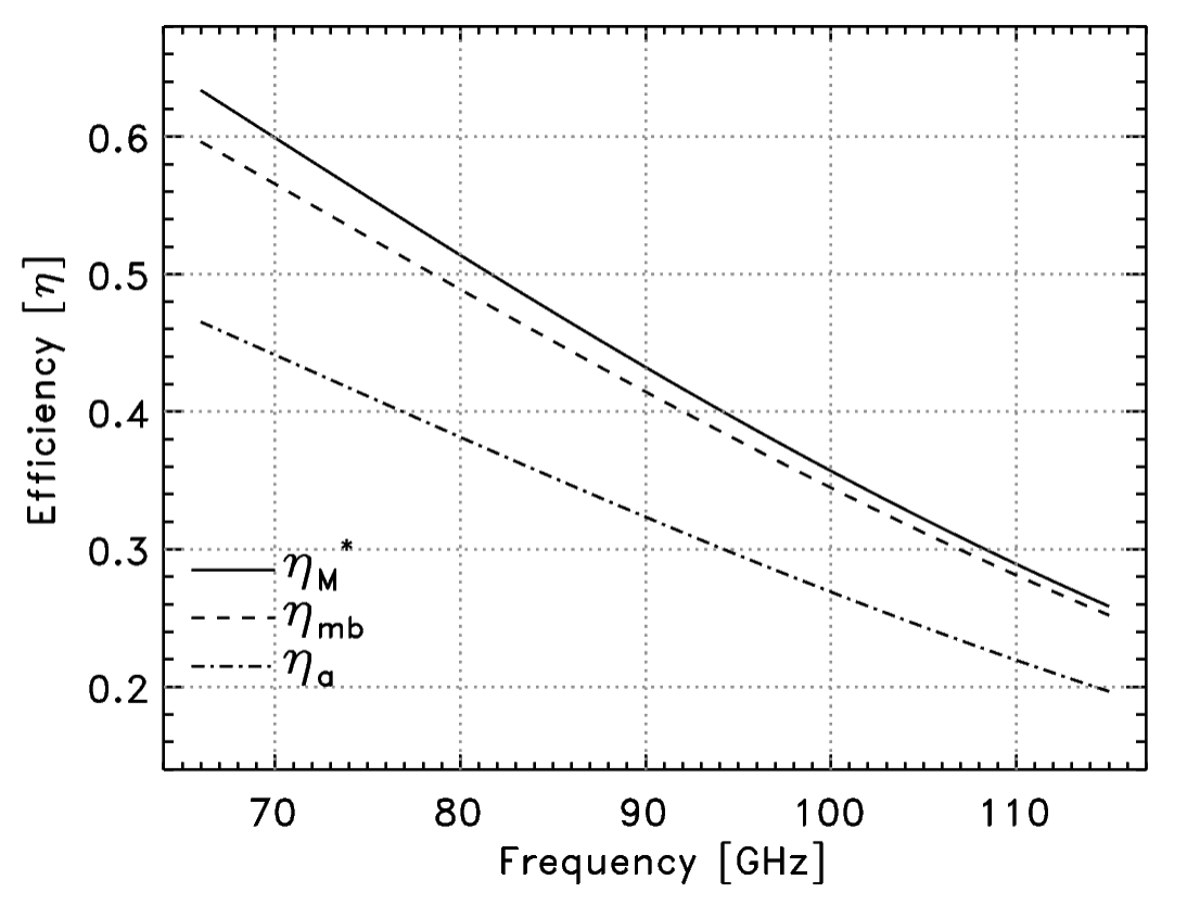
Figure 4: The estimated efficiencies of the GBT as a function of frequency assuming an effective surface error of 235$\mu$m and a beam size parameter of $\kappa=1.2$. The dashed-dotted line is the aperture efficiency. The main-beam efficiency is shown by the dashed line, while the corrected main-beam efficiency is given by the solid line.

Based on the above equations, $\eta_{M}^{*}$ and $\eta_{fss}$ can be computed as a function of frequency for the GBT (Figure 4). These derived efficiencies are not sensitive to the value $c_{\sigma}$ since it cancels out in equation (31). The above equations reduce to

$$\eta_{M}^{*}=\left(1+\frac{16\ln(2)}{\pi^{2}\kappa^{2}}\left[\frac{1}{\eta_{a}}-\frac{1}{\eta_{0}}\right]\right)^{-1}.$$ (34)

This is a useful general expression that only depends on the beam parameter ($\kappa$) and the aperture efficiency, which is given by the surface rms $\epsilon$. Equations (32) and (33) are derived assuming $\delta<1$, i.e., at wavelengths for which the telescope performs well. In the case of $\delta>1$, the additional terms required in the analysis cancel out when computing $\eta_{M}^{*}$, allowing equation (34) to be useful for all values of $\delta$.

The forward spillover and scatter efficiency can also be expressed theoretically based only on the telescope $\kappa$ and $\epsilon$ parameters;

$$\eta_{fss}=\frac{0.8899\kappa^{2}\eta_{a}}{\eta_{l}\eta_{M}^{*}}.$$ (35)

At 86 GHz the derived efficiencies are $\eta_{M}^{*}=0.465\pm 0.035$ and $\eta_{fss}=0.965\pm 0.020$, adopting $\kappa=1.2$ and $\epsilon=235\mu$m.

4.4 Antenna Pattern

By assuming a Gaussian approximation for the main-beam and the error pattern and using the equations in the previous sub-section, the physical scale ($c_{\sigma}$, correlation radius) associated with the error pattern can be estimated. Baars (1973) discusses the method for deriving this parameter based on the measured beam efficiencies of small sources and a large extended source. The correlation radius is given by

$$c_{\sigma}=\frac{2\lambda}{\pi\theta_{S}}\left[-\ln\left(\frac{\eta_{B0}-\eta_{B}^{\prime}}{\eta_{B0}-\eta_{mb}}\right)\right]^{0.5},$$ (36)

where the main-beam efficiency $\eta_{mb}$ is given by equation (9) and $\eta_{B0}$ is the idealized main-beam efficiency at long wavelengths ($\eta_{B0}\simeq 0.905\,[0.71\times 1.274]$ for the GBT). The value $\eta_{B}^{\prime}$ is the beam efficiency measured for an extended source with angular size $\theta_{S}$, where $\theta_{mb}<\theta_{S}<\theta_{E}$.

Using measurements of Jupiter ($\theta_{S}=43^{\prime\prime}$) at 86–89 GHz, $\eta_{B}^{\prime}=\eta_{\rm Jupiter}=0.53$. At the default Argus calibration frequency of 86 GHz, $\eta_{a}=0.347$ and $\eta_{mb}=0.442$ (assuming typical 235$\mu$m surface errors). Based on these values and using equation (36), a value of $c_{\sigma}\simeq 500$ cm is derived, which corresponds to an angular scale of $76^{\prime\prime}$. In comparison, the GBT panels are $\sim 250\times 200$ cm in size (Schwab & Hunter 2010), so the derived correlation radius corresponds to a size of about 2 panels. The Gravity Zernike model and the AutoOOF Thermal Zernike coefficients correct for significantly larger scale distortions of order 20m across the dish. This suggest that the correlation radius should be fairly insensitive to the Zernike coefficients.

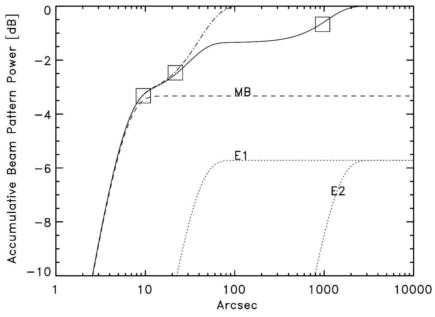
Figure 5: The accumulative beam pattern power as a function of radius at 86 GHz. The boxes show the measured beam efficiencies for small sources, Jupiter, and the Moon. The dashed-dotted line is a fit assuming only one Gaussian component for the error pattern, while the solid line shows the fit using two Gaussian components for the error pattern. The dashed and dotted lines show the accumulative power as a function radius for the individual components (main-beam [MB] and error-beam components [E1, E2], see Table 1). The power is plotted in units of dB ($10\log_{10}[P]$).

By using observations of the Moon, the amount of power on larger spatial scales outside of the error pattern measured with Jupiter can be determined. Measurements of the Moon using Argus yield $\eta_{\rm Moon}=0.81\pm 0.038$ at 88.9 GHz and $0.82\pm 0.044$ at 110.0 GHz. There is no evidence for any significant frequency dependency with $\eta_{\rm Moon}$ within the 3mm band. Based on the weighted average of these observations, a value of $\eta_{\rm Moon}=0.814\pm 0.029$ is adopted. This value is significantly lower than $\eta_{fss}$ and what would be expected by integrating over the main-beam pattern and the error pattern implied by the observations of Jupiter (dashed-dotted line in Figure 5). This suggests an additional error component to the beam pattern. The Jupiter and Moon data are fitted with a double Gaussian error pattern with the results shown in Figure 5 and Table 1. The data were fitted using three free parameters, which are the size scales associated with each of the two components of the error pattern ($c_{E1}=700\pm 200$ cm and $c_{E2}=20\pm 10$ cm) and the relative amount of power contained within the two components ($A_{E1}\theta_{E1}^{2}/(A_{E2}\theta_{E2}^{2})=1.0\pm 0.5$).

4.5 Extended Source Calibration

The planets can be used to derive beam efficiencies of the telescope. The main-beam efficiency measured for a planet of known brightness temperature $T_{b}$ and diameter $\theta_{S}$ is given by

$$\eta_{mb}=\frac{T_{a}^{\prime}}{J_{\nu}(T_{b})[1-\exp(-x^{2})]},$$ (37)

where $x=\sqrt{\ln\,2}(\theta_{S}/\theta_{mb})$ (e.g., Kramer 1997). This equation is useful for the small angular-size planets, such as Mars and Uranus which are the two primary calibrator sources used for mm astronomy. The value of $x$ assumes a Gaussian telescope beam, which is a good approximation for planet disks smaller than $\theta_{mb}$. For disks $\theta_{S}/\theta_{mb}\,\lower 2.0pt\hbox{${>\atop\hbox{\raise 4.0pt\hbox{$\sim$}}}$}\,1$, then using a Bessel function for telescope beam is more appropriate than a Gaussian. For very large sources $\theta_{S}/\theta_{mb}>3$, such as Jupiter or the Moon, then approximation given by equation (11) is applicable.

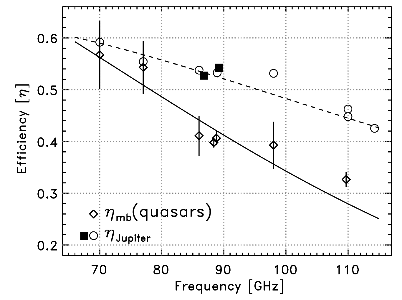
Figure 6: The diamonds show the main-beam efficiencies measured using quasars, and the solid line corresponds to an average ratio of $\eta_{mb}/\eta_{a}=1.274$. The solid squares show measurements of Jupiter for two sessions when the telescope had good aperture efficiencies. The circles represent $\eta_{\rm Jupiter}$ corrected for the relative aperture efficiencies between different sessions. The dashed line is an empirical relationship fitted to the circles and solid squares representing $\eta_{\rm Jupiter}$ as a function of frequency.

Figure 6 compares the measured main-beam efficiencies ($\eta_{mb}$) for quasars to the beam efficiency measured for Jupiter ($\eta_{\rm Jupiter}$). The values of $\eta_{\rm Jupiter}$ are larger than $\eta_{mb}$ given that measurements of Jupiter include significant power from the antenna error pattern (§4.4). For small sources, variations in $\eta_{a}$ directly correlate with variations in $\eta_{mb}$ (equation 9) as expected for different observing sessions, depending on the conditions and the quality of the telescope corrections. Since Jupiter is much larger than the beam size, one could expect the measured $\eta_{\rm Jupiter}$ values to be fairly independent of the detailed telescope corrections. However, we found significant variations of $\eta_{\rm Jupiter}$ that correlated roughly linearly with $\eta_{a}$. The solid squares for Jupiter in Figure 6 were derived in sessions with good aperture efficiencies consistent with the adopted $\epsilon=235\mu$m derived here and used in §4.2–4.4. For session TGBT17B_502_01, both $\eta_{\rm Jupiter}$ and $\eta_{a}$ were 10% lower, and for session AGBT18B_370_02 both $\eta_{\rm Jupiter}$ and $\eta_{a}$ were about 20% lower than the nominal values. After scaling by the relative aperture efficiencies between sessions, the $\eta_{\rm Jupiter}$ values are consistent between sessions (open circles and solid squares in Figure 6). This plot potentially embeds information on the telescope error beam as a function of frequency (following the analysis in §4.4). However, additional well-calibrated scanning observations of Jupiter and the Moon are needed to more accurately constrain the antenna pattern of the GBT at high frequency.

5 Discussion

Table 2 shows the derived GBT performance values at 86 GHz. This memo presents relationships to compute $\eta_{a}$, $\eta_{mb}$, $\eta_{M}^{*}$, and $\eta_{fss}$ as a function of frequency based only on the effective surface error $\epsilon$ and the beam size $\kappa$ parameter. These relationships assume the dominate effects on performance of the telescope are related to surface deformations using the Ruze equations. In cases of low inferred aperture efficiencies that are due to pointing and/or focus errors, for example, these relationships that depend on $\eta_{a}$ may not be applicable.

There is a fairly wide-range of derived aperture efficiencies for the GBT at 3 mm depending on the weather conditions and the quality of the telescope corrections. Sessions with unreasonably low source amplitudes were not used in this analysis. For the 143 observations from 86–90 GHz presented here, $\eta_{a}=0.33\pm 0.05$, but it is not unusual to measure values as low as $\eta_{a}\simeq 0.2$ from archival data. The analysis of the archival data has highlighted the challenges for users, at times, to obtain quality data. The default pointing/focus/OOF software solutions are not always appropriate, and software updates could improve the ability to derive reasonable solutions in less than ideal weather conditions. Winds can be particularly troublesome during the OOF observations. In these cases, the derived OOF corrections could significantly decrease the performance of the telescope. It is recommended to use the Ka+CCB system for deriving the OOF corrections, when it is available on the telescope, since winds have a smaller effect at Ka-band frequencies (30 GHz) given the larger beam size, and the Ka+CCB system provides much higher signal-to-noise measurements than can be achieved at W-band frequencies.

For measuring efficiencies, more reliable results are obtained by slewing the over the source instead of using the NOD or ON$-$OFF observing routines. By slewing over the source, the background sky signal as a function of time is more accurately determined. For small sources, the aperture efficiency is given by the peak signal of the scan, while the main-beam efficiency is derived by integrating over the source profile contained within the main-beam.

We recommend absolute calibration to be carried out on bright quasars, taking advantage of the on-line ALMA calibrator catalog. Planets can also be used, but the size of the planet should be less than the beam size to avoid complications in estimating the effects of source coupling with the antenna beam pattern. In terms of brightness and size, only Mars is suitable for main-beam efficiency measurements (when Mars is not near the Earth). Measurements of Jupiter and the Moon can be used to constrain the error patterns of the telescope beam.

6 References

• Baars, J. W. M., 1973, The Measurement of Large Antennas with Cosmic Radio Sources, IEEE Tran. on Antennas and Propagation, Vol AP-21, No. 4, 461

• Braatz, J. 2009, Calibration of GBT Spectral Line Data in GBTIDL v2.1

• Butler, B. 2012, Flux Density Models for Solar System Bodies in CASA, ALMA Memo #594

• Frayer, D. T. 2017, The GBT Beam Shape at 109 GHz, GBT Memo #296

• Frayer, D. T., Ghigo, F., & Maddalena, R. J. 2018, The GBT Gain Curve at High Frequency, GBT Memo #301

• Frayer, D. T., et al. 2015, The GBT 67–93.6 GHz Spectral Line Survey of Orion-KL, AJ, 149, 162

• Kramer, C. 1997, Calibration of spectral line data at the IRAM 30m radio telescope

• Kutner, M. L. & Ulich, B. L. 1981, Recommendations for calibration of millimeter-wavelength spectral line data, ApJ, 250, 341

• Maddalena, R. J. 2010, Theoretical Ratio of Beam Efficiency and Aperture Efficiency, GBT Memo # 276

• Mangum, J. G. 1993, Main-beam efficiency measurements of the Caltech Submillimeter Observatory, PASP, 105, 117

• Mangum, J. G. 1999, Equipment and Calibration Status for the NRAO 12 Meter Telescope

• Schwab, F.R. & Hunter, T.R. 2010, Distortions of the GBT Beam Pattern Due to Systematic Deformations of the Surface Panels, GBT Memo #271

• Srikanth, S. 1989a, Spillover Noise Temperature Calculations for the Green Bank Clear Aperture Antenna, GBT Memo #16

• Srikanth, S. 1989b, More on the Spillover Noise Temperature Comparisons for the Green Bank Telescope GBT Memo #19

• Wilson, T. L., Rohlfs, K., & Hüttemeister, S. 2010, Tools of Radio Astronomy, Fifth Ed. (Springer-Verlag Berlin Heidelberg)

7 Tables

Table 1: 86GHz Beam Pattern Measurements

	Relative Amplitude	$\theta$(FWHM)	Fractional Powera
MB	1.0	8.64 arcsec	0.464
E1	$0.014\pm 0.004$	$55\pm 16$ arcsec	$0.268\pm 0.134$
E2	$(1.2\pm 0.6)\times 10^{-5}$	$1900\pm 950$ arcsec	$0.268\pm 0.134$

^aFractional power does not include the estimated 5% of total power that resides outside of the main-beam (MB) and error components (Fig. 5), which is given by $(1-\eta_{fss}\,\eta_{l})$.

Table 2: 86GHz GBT Efficiency and Calibration Parameters

Dish Diameter	D	100 m
RMS Surface Accuracy	$\epsilon$	$235\pm 15\,\mu$m
Beam Size Parameter	$\kappa$	$1.20\pm 0.02$
Aperture Efficiency	$\eta_{a}$	$0.347\pm 0.032$
Main-Beam Efficiency	$\eta_{mb}$	$0.442\pm 0.043$
Corrected Main-Beam Efficiency	$\eta_{M}^{*}$	$0.465\pm 0.035$
Jupiter Beam Efficiency($43^{\prime\prime}$diameter)	$\eta_{\rm Jupiter}$	$0.53\pm 0.05$
Moon Beam Efficiency ($32^{\prime}$ diameter)	$\eta_{\rm Moon}$	$0.814\pm 0.029$
Rear Spillover Efficiencya	$\eta_{l}$	$0.985\pm 0.015$
Forward Spillover Efficiencyb	$\eta_{fss}$	$0.965\pm 0.020$

^aPower in the forward $2\pi$ direction. ^bFactional power in the forward direction inside the $\sim 1^{\circ}$ diameter error pattern.

8 Appendix A

The listing of GBT observing sessions used in the data analyses is provided.

Table 3: GBT Observing Sessions

GBT Project	Session	Date
AGBT17A_304	02	2017.02.15
AGBT17A_304	03	2017.02.27
AGBT17A_304	05	2017.03.13
AGBT17A_304	06	2017.03.23
AGBT17A_304	07	2017.04.09
AGBT17A_304	08	2017.04.10
AGBT17A_304	09	2017.04.11
AGBT17B_151	02	2017.10.16
AGBT17B_151	03	2017.10.19
AGBT17B_151	04	2017.11.12
AGBT17B_151	05	2017.11.14
AGBT17B_151	07	2017.11.18
AGBT17B_151	12	2017.12.15
AGBT17B_151	13	2017.12.21
AGBT17B_151	15	2018.01.16
AGBT17B_151	18	2018.01.26
AGBT17B_151	19	2018.01.27
AGBT17B_151	20	2018.01.31
AGBT17B_151	23	2018.02.03
AGBT17B_151	24	2018.02.26
AGBT17B_151	25	2018.02.27
TGBT17B_502	01	2018.04.06
AGBT17A_245	04	2018.04.06
AGBT17A_245	05	2018.04.09
AGBT18B_370	01	2018.12.09
AGBT18B_370	02	2019.03.24

9 Appendix B

The efficiencies are explicitly defined in their integral form following the conventions of Kutner & Ulich (1981). The rearward scattering and spillover efficiency is

$$\eta_{rss}=\frac{\int\!\!\int_{2\pi}P_{n}(\Omega)d\Omega}{\int\!\!\int_{4\pi}P_{n}(\Omega)d\Omega},$$ (38)

where $P_{n}$ is the normalized antenna power pattern ($P_{n}(0)=1$) and $2\pi$ is in the forward (on-sky) direction. The efficiency $\eta_{l}=\eta_{r}\eta_{rss}$, where the ohmic efficiency is $\eta_{r}\simeq 1.0$. The forward scattering and spillover efficiency is

$$\eta_{fss}=\frac{\int\!\!\int_{\Omega_{D}}P_{n}(\Omega)d\Omega}{\int\!\!\int_{2\pi}P_{n}(\Omega)d\Omega},$$ (39)

where $\Omega_{D}$ is the antenna diffraction pattern, including the error pattern.

The main-beam efficiency is given by

$$\eta_{mb}=\frac{\int\!\!\int_{\Omega_{mb}}P_{n}(\Omega)d\Omega}{\int\!\!\int_{4\pi}P_{n}(\Omega)d\Omega},$$ (40)

where $\Omega_{mb}$ is the main-beam lobe. Assuming a Gaussian beam, the integral $\int\!\!\int_{\Omega_{mb}}P_{n}(\Omega)d\Omega=1.133\theta_{FWHM}^{2}$. Although the main-beam lobe is well approximated by a Gaussian, the antenna pattern at larger radii is not. For a circular aperture radio dish, the antenna pattern can be represented by a Bessel function (e.g., Wilson, Rohlfs, & Hüttemeister 2010), and the relative strength of the main-beam lobe to the side-lobes depend on the feed taper. In general, the standard integral limit for $\Omega_{mb}$ is at the diameter corresponding to the beam width of the first null (BWFN) for computing $\eta_{mb}$. Assuming typical feed tapers used in radio astronomy and adopting a Bessel function approximation for the beam pattern, $BWFN\approx 2.7\theta_{FWHM}$.

The corrected main-beam efficiency is

$$\eta_{M}^{*}=\frac{\int\!\!\int_{\Omega_{mb}}P_{n}(\Omega)d\Omega}{\eta_{r}\int\!\!\int_{\Omega_{D}}P_{n}(\Omega)d\Omega},$$ (41)

which is $\eta_{M}^{*}=\eta_{mb}/(\eta_{l}\,\eta_{fss})$. For sources larger the beam size, the measured beam efficiency depends on the coupling of the source to the antenna beam pattern (equation 10). The coupling efficiency $\eta_{c}$ is

$$\eta_{c}=\frac{\int\!\!\int_{\Omega_{\rm Source}}P_{n}(\Psi-\Omega)B_{n}(\Psi)d\Psi}{\int\!\!\int_{\Omega_{D}}P_{n}(\Omega)d\Omega},$$ (42)

where $\Psi$ is the source angle on the sky and $B_{n}$ is the normalized source brightness temperature ($B_{n}(0)=1$). This definition is consistent with Kutner & Ulich (1981) where $T_{R}^{*}=\eta_{c}\,T_{S}$.

10 Figures