Hyperbolic Fracton Model, Subsystem Symmetry, and Holography II: The Dual Eight-Vertex Model

Abstract

The discovery of fracton states of matter opens up an exciting, largely unexplored field of many-body physics. Certain fracton states’ similarity to gravity is an intriguing property. In an earlier work Yan (2019), we have demonstrated that a simple fracton model in anti-de Sitter space satisfies several major holographic properties. In this follow-up paper, we study the eight-vertex model dual to the original model. The dual model has the advantage of illuminating the mutual information and subsystem charges pictorially, which helps to reveal its connections to various other topics in the study of holography and fracton phases. At zero temperature, the dual eight-vertex model is a discrete realization of the bit-thread model, a powerful tool developed to visualize holography. The bit-thread picture combined with subsystem charges can give a quantitative account of the isometry between the bulk and the boundary at finite energy, which is also a key issue for holography. The black hole microscopic degrees of freedom can be identified in this picture, which turn out to be encoded non-locally on the horizon. The eight-vertex model proves to be a very helpful venue to improve our understanding of the hyperbolic fracton model as a toy model of holography.

I Introduction

The recent discovery of fracton states of matter Chamon (2005); Yoshida (2013); Bravyi et al. (2011); Haah (2011); Vijay et al. (2015, 2016); Pretko (2017a, b); Nandkishore and Hermele (2019) is an exciting development in many-body physics. These models feature exotic excitations with constrained mobility dubbed “fractons” , and gauged or ungauged subsystem symmetries. The fracton topological orders are also beyond our conventional knowledge of topological orders. The fracton states present many new challenges, including model building Shirley et al. (2018); Slagle et al. (2019); Tian et al. (2018); You (2019); Song et al. (2019); You et al. (2018), experimental realizations Slagle and Kim (2017); Hsieh and Halász (2017); Halász et al. (2017); Ma et al. (2017); You and von Oppen (2018); Yan et al. (2019); Benton et al. (2016), proper classification scheme Shirley et al. (2018); Pai and Hermele (2019); Gromov (2018); Shirley et al. (2019a), quantum-information application Schmitz et al. (2018); Kubica and Yoshida (2018); He et al. (2018); Ma et al. (2018); Schmitz (2018); Schmitz et al. (2019); Pai et al. (2019); Shirley et al. (2019b), and its connection to other areas of physics Pretko (2017c); Pretko and Radzihovsky (2018); Pai and Pretko (2018); Pretko and Radzihovsky (2018); Gromov (2019); Yan (2019).

An intriguing aspect of fracton states of matter is their similarity to gravity Pretko (2017c); Gromov (2019); Slagle et al. (2019). The fracton excitations can be described as charges of the generalized rank-2 U(1) gauge theories Xu (2006); Rasmussen et al. (2016); Pretko (2017a, b); Slagle and Kim (2017); Prem et al. (2018); You et al. (2018); Bulmash and Barkeshli (2018); Ma et al. (2018); Slagle et al. (2018); Shirley et al. (2018); Devakul et al. (2019), where the electric and gauge fields take the form of symmetric matrices and have modified Gauss conservation laws. These theories have been shown to exhibit behaviors similar to general relativity, and are indeed the linearised limit of certain gravitational/elasticity theories Pretko (2017c); Pretko and Radzihovsky (2018); Gromov (2019).

Along this line, a very simple classical fracton toy model in anti-de Sitter space was shown to satisfy a few major holographic properties Yan (2019). The holographic principle Hooft (1974); Susskind (1995) and anti-de Sitter/conformal field theory (AdS/CFT) correspondence Maldacena (1999); Witten (1998), as a ground-breaking framework to demystify quantum gravity, have been front line for the high energy theory community for a few decades Gubser et al. (1998); Aharony et al. (2000, 2008); Klebanov and Polyakov (2002); Hawking (2005); Guica et al. (2009). It is also a powerful tool-set to understand strongly coupled systems Hartnoll et al. (2016); Pires (2014); Zaanen et al. (2015); Nastase (2017); Qi (2013); Gu et al. (2016); Lee and Qi (2016). In this context, the hyperbolic fracton model satisfies the celebrated Ryu-Takayanagi formula Ryu and Takayanagi (2006a, b), and also has the correct subregion duality Van Raamsdonk (2009). Its construction has a lot of similarities to the holographic toy models built from tensor networks Swingle (2012); Pastawski et al. (2015); Almheiri et al. (2015); Yang et al. (2016); Hayden et al. (2016); Qi and Yang (2018); Harlow (2017).

This paper, as the second of the duology on the hyperbolic fracton model, studies the dual eight-vertex model of the original model, which has the advantage of visualizing the mutual information and subsystem fluxes.

It helps to address a few key unanswered questions following the initial discovery. One question is whether the hyperbolic fracton model is equivalent to any other known holographic models/theories. This turns out to be true. The dual eight-vertex model is a discrete realization of the bit-thread model Freedman and Headrick (2017); Cui et al. (2018); Harper et al. (2018); Headrick and Hubeny (2018); Chen et al. (2018), which was proposed as a very powerful framework to understand holography. It treats the non-local “flow of information” instead of local fields as the elementary physical quantity. From this perspective many holographic properties of entanglement entropy have an intuitive, pictorial derivation.

Another question is about holography beyond the ground states. This was not discussed much in the previous work. Here equipped with the bit-thread picture and the concept of subsystem charges, a detailed analysis is presented. We show that “isometry”, the requirement from holography that the boundary uniquely determines the bulk, is violated only by a small amount at low energy levels, and all violating cases can be determined.

The bit-thread and subsystem charge language also help us to identify the black hole microscopic degrees of freedom (dofs), which is encoded non-locally on the horizon, and also the AdS boundary. Intriguingly even though the black hole set-up is very primitive, it yields qualitatively correct behavior of how a boundary observer can distinguish the microstates Bao and Ooguri (2017).

This work and Ref.Yan (2019) form a relatively comprehensive investigation of the classical toy hyperbolic fracton model. In the outlook, we discuss future directions beyond this simple toy model, which could be an interesting program for condensed matter physics, and hopefully provide some insights in high energy theory too.

This paper is arranged as follows: Sec. II briefly reviews the results from Ref. Yan (2019); Sec. III describes the dual eight-vertex model on the Euclidean lattice and Sec. IV on the hyperbolic lattice;

The first major result of this work, Sec. V, explains the eight-vertex model as a realization of the bit-thread model. It is then utilized to derive results documented in the two following sections: Sec. VI analyzes the isometry properties of the excited states; Sec. VII describes the black hole microscopic degrees of freedom in the model;

Finally Sec. VIII summarizes this paper and gives an outlook of possible future directions.

II Brief Review of the Holographic Hyperbolic Fracton Model

In this section we recapitulate the classical hyperbolic fracton model and its holographic properties, which are the main result of Ref. Yan (2019). Interested readers are recommended to refer to it for more details.

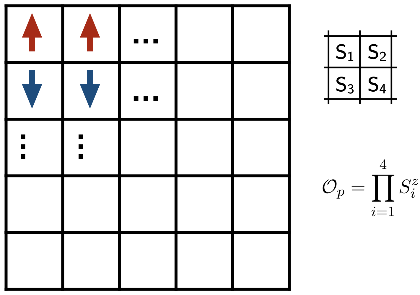
(a) Square Lattice

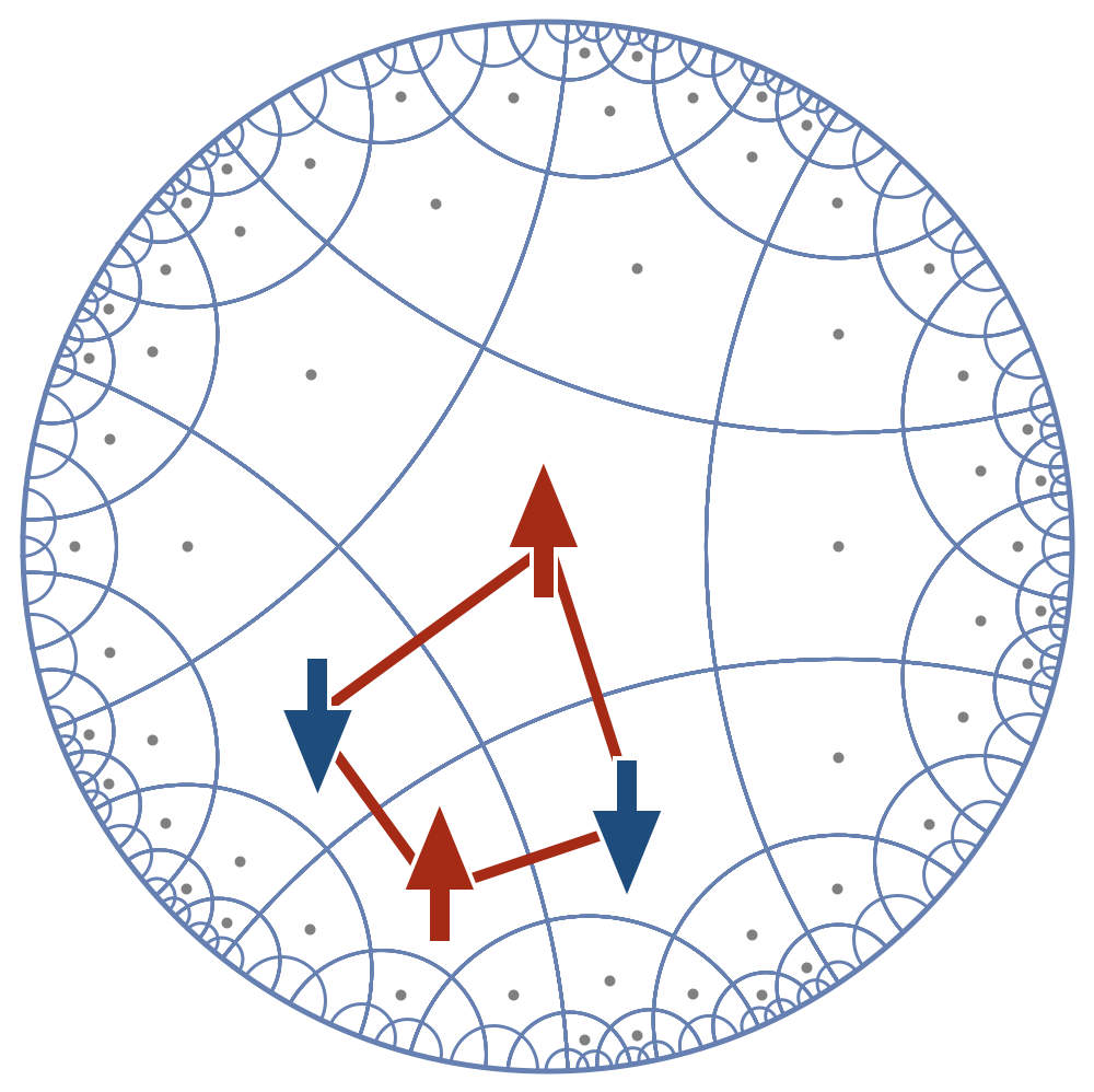
(b) Hyperbolic lattice

Figure 1: The fracton model (Eq. (2)) on the Euclidean and hyperbolic lattice. (a) The model defined on the Euclidean lattice. (b) The model defined on the hyperbolic lattice of (5,4) tessellation. Spins sit at the centers of the pentagons. The plaquette operator is defined on each cluster of the four corner-sharing pentagons as shown by the red box.

The classical fracton model can be defined on both the Euclidean and hyperbolic (negatively curvatured, or AdS) lattice based on uniform square and pentagon tessellations shown in Fig. 1a, 1b. In the later case, the hyperbolic lattice is obtained by the (5,4) tessellation, i.e., tiling the 2D AdS space with pentagons, with four pentagon sharing every corner. An Ising spin of value $S_{i}^{z}=\pm 1$ is placed at the center of each square in the Euclidean lattice or pentagon in the hyperbolic lattice. The operator

$$\mathcal{O}_{p}=\prod_{i=1}^{4}S^{z}_{i},$$ (1)

is defined for each four-spin cluster, where $i$ runs over its four sites. Such a cluster on the hyperbolic lattice is shown by the red rectangle in Fig. 1b. The Hamiltonian for both models is

$$\mathcal{H}_{\textsf{spin}}=-\sum_{p}\mathcal{O}_{p}\;,$$ (2)

where the sum runs over all four-spin clusters.

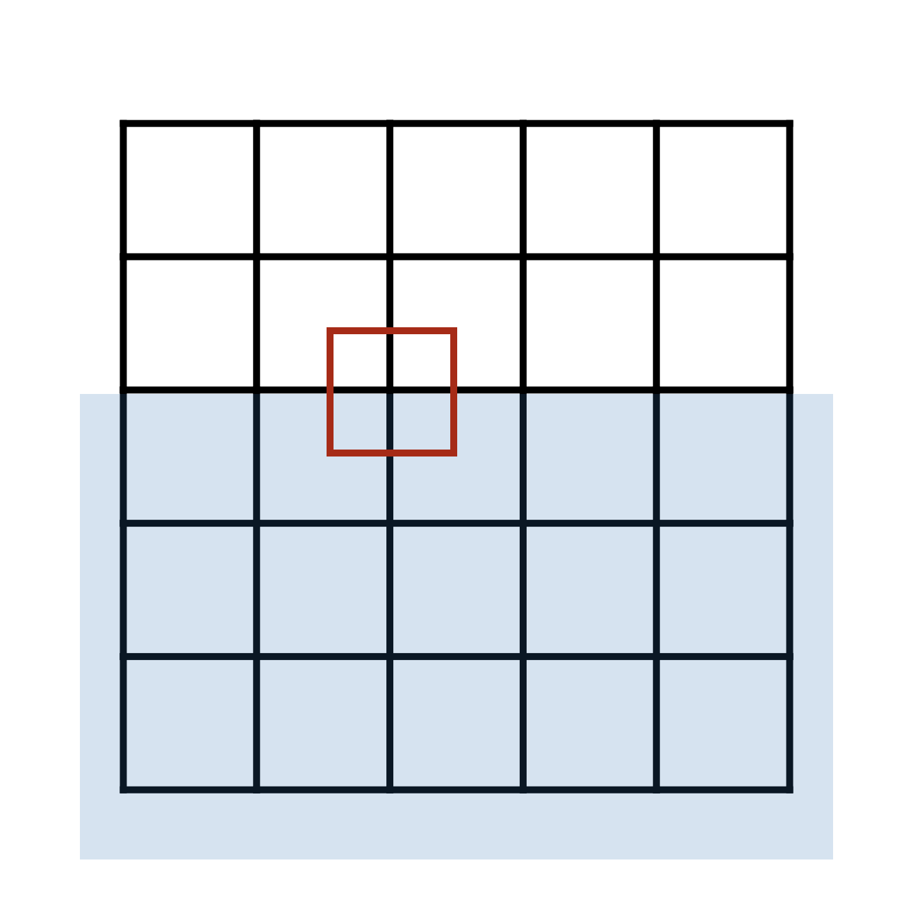
(a)

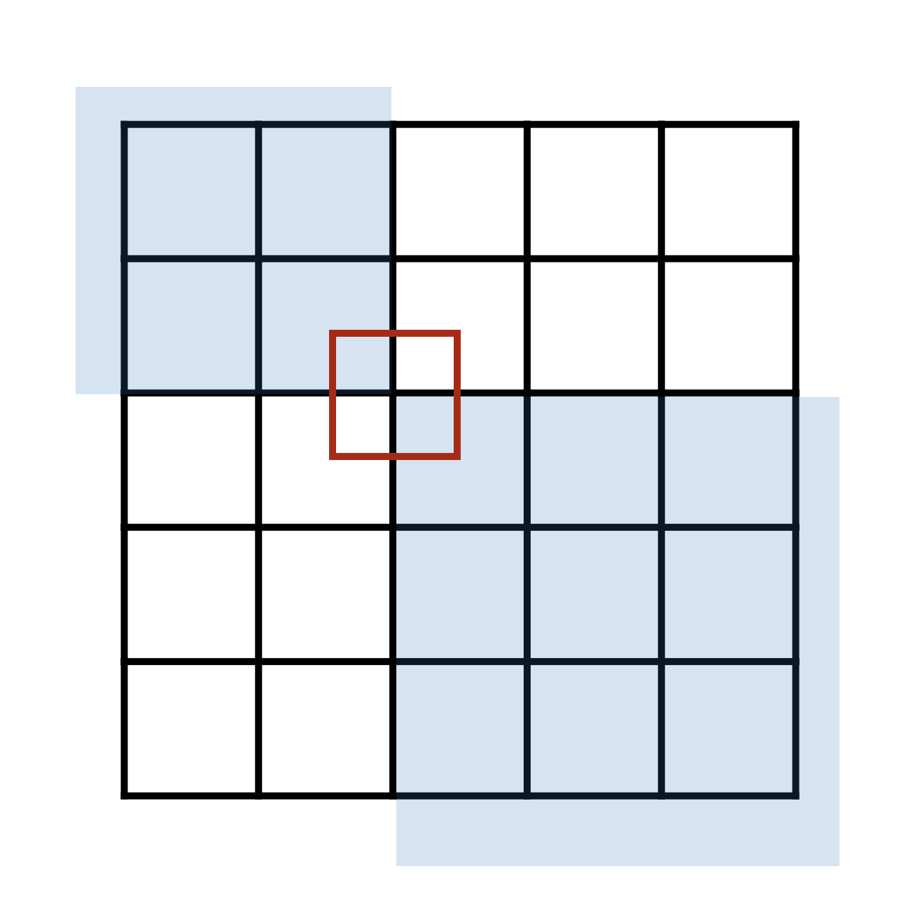
(b)

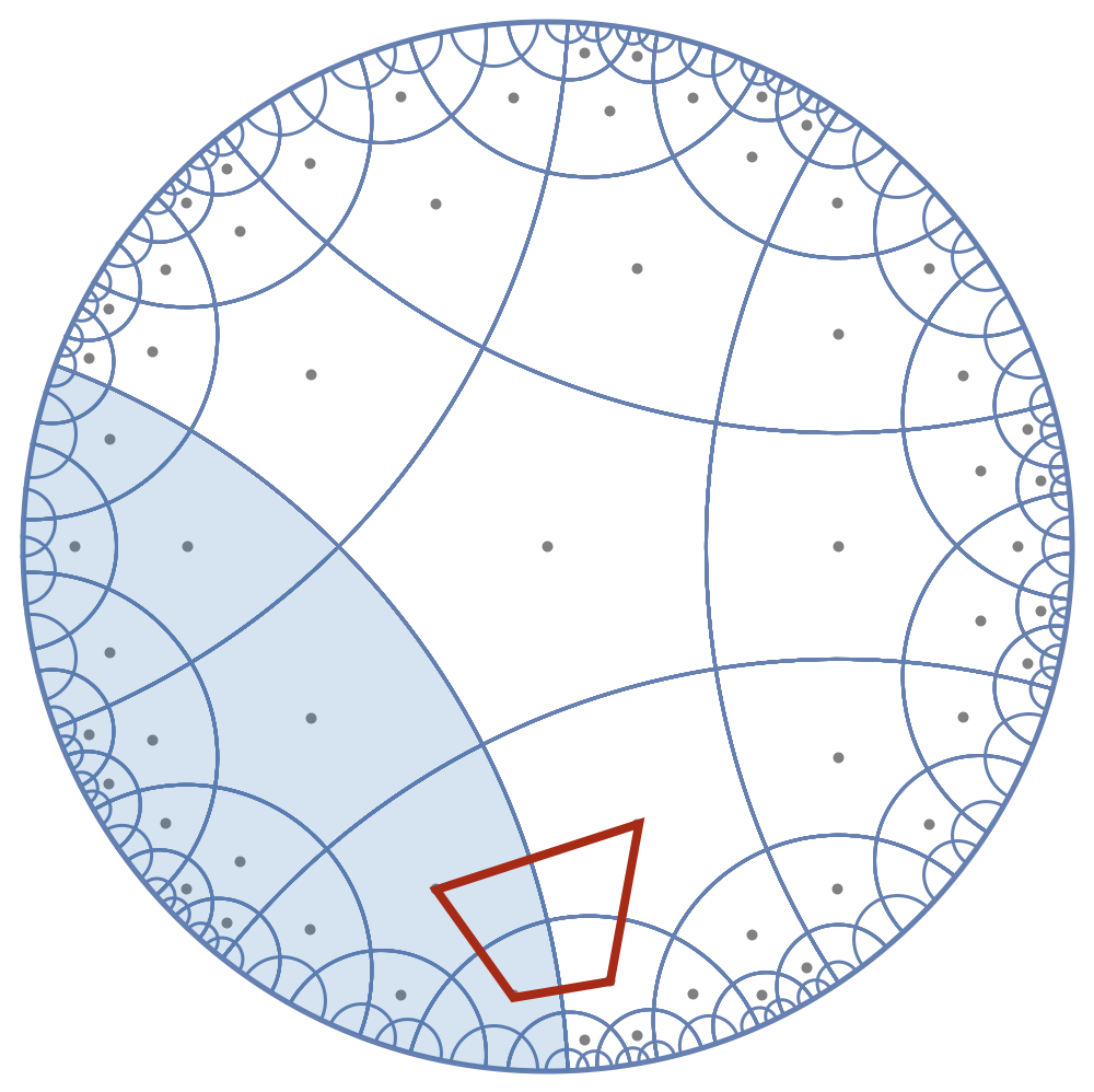
(c)

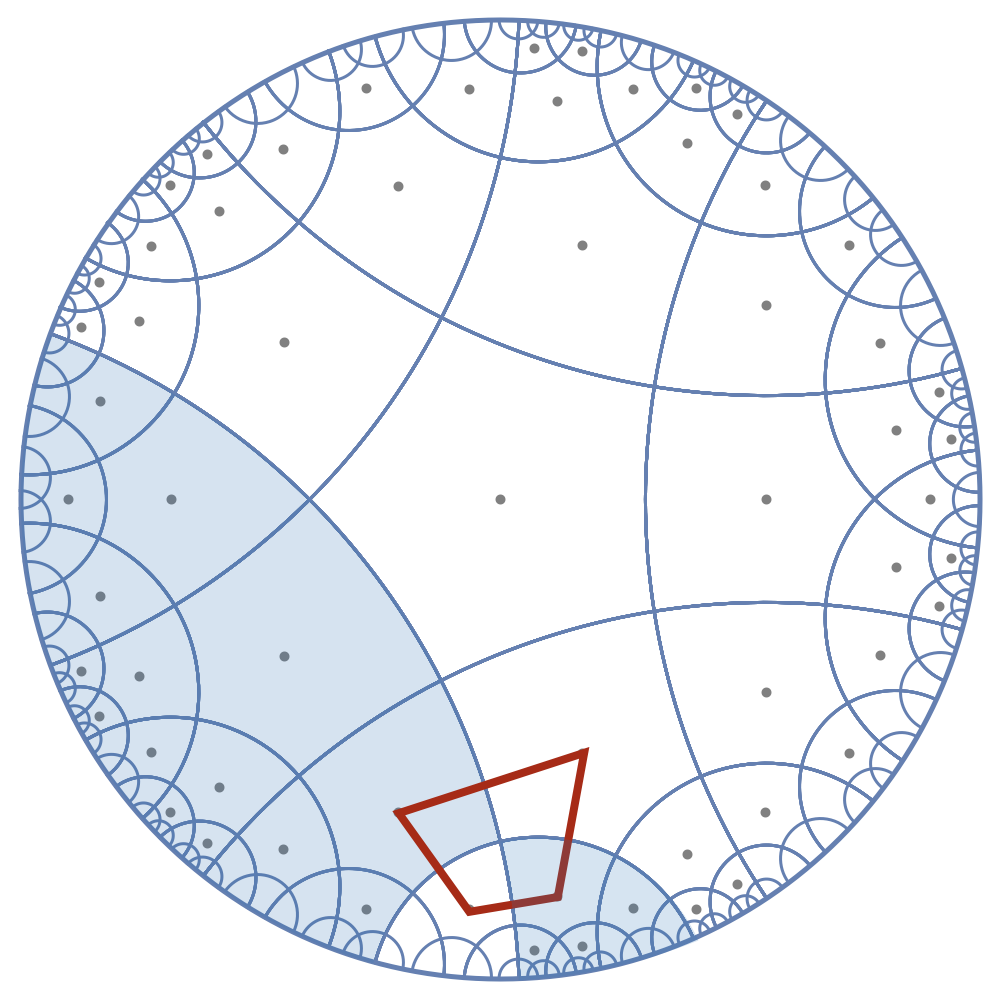
(d)

Figure 2: Ground state degeneracy of the fracton models on the Euclidean lattice (a, b) and hyperbolic lattice (c, d). The blue region are the spins flipped from the original ground state. Note that the four-spin clusters always have even number of spins flipped.

An essential property of these models is their subsystem symmetry. Note that the pentagon’s edges define some geodesics, i.e., straight lines in $x-$ or $y-$ direction on the Euclidean lattice and arcs intersecting the disk boundary perpendicularly on the hyperbolic disk. The energy of the system is invariant under the operation of flipping all spins on either side of a chosen geodesic. By starting from any given ground state and consecutively applying such operations for different geodesics, all ground states can be explicitly constructed. Thus, the ground state degeneracy is proportional to $2^{\text{number of geodesics}}$, which is also proportional to $2^{\text{boundary size}}$. This feature is dubbed “subsystem symmetry” in literature Vijay et al. (2016); You et al. (2018); Shirley et al. (2019a). It is a symmetry in-between local and global, and the origin of many exotic features of fracton models, including the holographic ones.

Ref. Yan (2019) has demonstrated the following holographic properties of the hyperbolic fracton model.

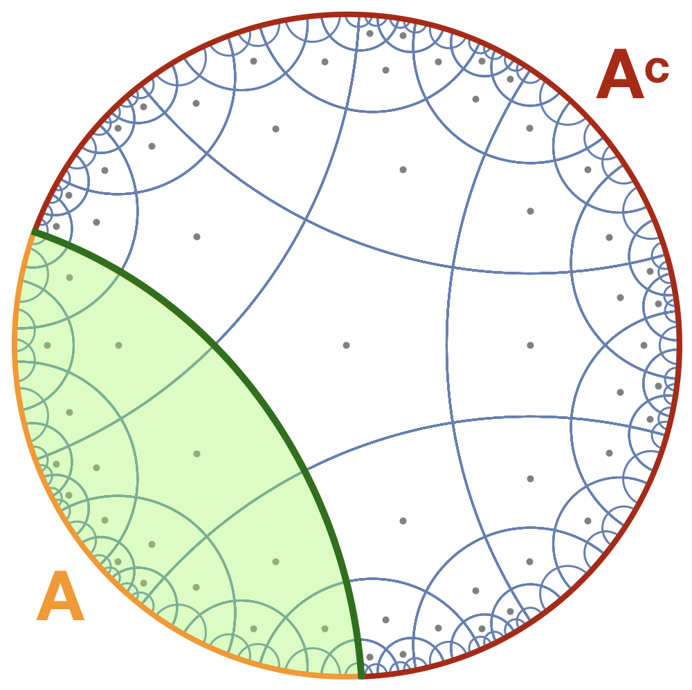
(a)

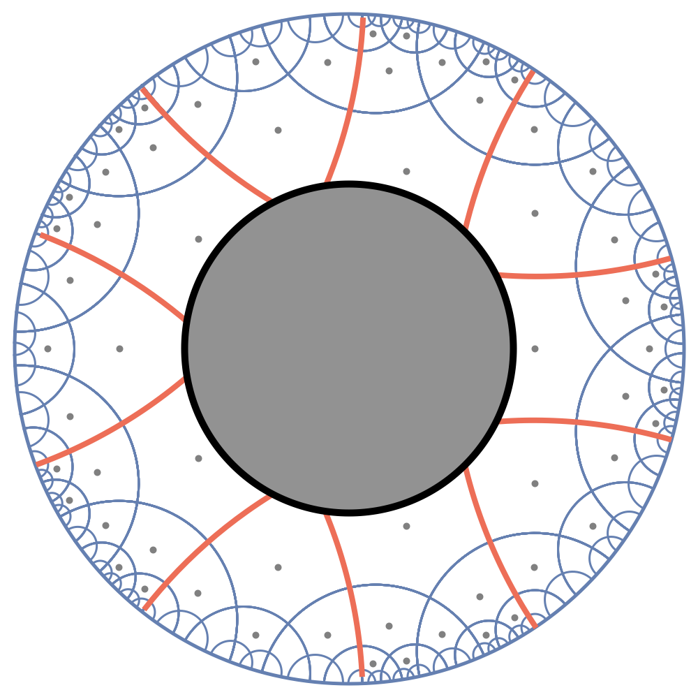
(b)

Figure 3: Holographic properties of the hyperbolic fracton model. (a): Sub-region duality and RT formula for mutual information. Give the boundary spins on segment $A$ (orange), the reconstructible bulk at $T=0$ are those in the minimal convex wedge colored in light green. The mutual information between boundary bipartition $A$ and $A^{c}$ (red) is proportional to the length of the minimal covering surface (dark green geodesic). (b): A black hole in the bulk. This naively defined black hole (dark gray region) has entropy proportional to its horizon area, or the number of orange geodesics.

Rindler reconstruction and subregion duality — For the hyperbolic fracton model defined by Eq. (2), given a spin configuration on a connected boundary segment, the bulk spins in a specific region (Fig. 3a) are determined unambiguously at zero temperature. This region, dubbed minimal convex wedge, agrees with the reconstructible entanglement wedge determined by Rindler reconstruction or subregion duality of holography Van Raamsdonk (2009).

Ryu-Takayanagi formula for mutual information — Given a bipartition of the boundary into two connected segments $A$ and $A^{c}$, their mutual information (the classical analog of entanglement entropy),

$$\I(A,A^{c})=S_{A}+S_{A^{c}}-S_{A\cup A^{c}},$$ (3)

obeys the Ryu-Takayanagi formula Ryu and Takayanagi (2006a, b):

$$\I(A,A^{c})=k_{\text{B}}\log 2\times|\gamma_{A}|\;.$$ (4)

where $|\gamma_{A}|$ is the area of the minimal covering surface, or in this case the length of the geodesic that separates $A$ and $A^{c}$ (Fig. 3a ).

Black hole entropy — A very naively defined black hole in the system, i.e., with a convex horizon but not changing the AdS geometry, has entropy proportional to the area of its horizon (Fig. 3b),

$$S_{\mathsf{BH}}=\frac{k_{\text{B}}\log 2}{2}\times|\gamma_{A}|\;.$$ (5)

which is consistent with the Hawking-Bekinstein black hole entropy Hawking (1975).

The difference of the factor $2$ between Eq. (4) and Eq. (5) is consistent, since by definition the mutual information is twice the entanglement entropy Yan (2019).

III Dual Eight Vertex Model on the Square Lattice

The main results of this paper revolve around a physically equivalent model of the hyperbolic fracton model — the dual eight-vertex model. Formulated in the language of arrows and vertices, it has the advantage of illuminating various connections between the hyperbolic fracton model and other established results in fracton phases and holography. In this section, we will describe the dual eight-vertex model, and discuss how it works as a straightforward demonstration of fracton-elasticity duality Pretko and Radzihovsky (2018, 2018); Gromov (2019) and subsystem charge Shirley et al. (2019a).

The square-lattice eight-vertex model is a canonical exactly solvable model Sutherland (1970); Fan and Wu (1970); Baxter (1971); Kadanoff and Wegner (1971); Baxter (2007). It is constructed by placing a binary arrow (left/right or up/down) on every edge of the square lattice, but only allowing vertex configurations of even number of arrows pointing in/out. The eight allowed vertex configurations are shown in Fig. 4. Under open boundary condition, each vertex can be independently assigned an energy cost $E_{i}\;(i=1,...,8)$ in the most generic case. Specifying $E_{i}$ completes the definition of the classical model.

vertex	1	2	3	4	5	6	7	8
winding number $N_{\mathsf{w}}$	0	0	0	0	1	1	-1	-1
net flux $C_{\mathsf{n}}$	0	0	0	0	4	-4	0	0
flux in $x$-direction $C_{\mathsf{x}}$	0	0	0	0	2	-2	2	-2
flux in $y$-direction $C_{\mathsf{y}}$	0	0	0	0	2	-2	-2	2

Figure 4: Vertex configurations in eight-vertex model and their winding numbers around the vertex center, total fluxes and fluxes in $x-$ and $y-$directions.

The eight-vertex model can be reformulated as an equivalent spin model that involves up to four-spin interactions Baxter (2007). The classical fracton model (Eq. (2)) described in Sec. II is a special case of the more general equivalence. The prescription of the duality is given below.

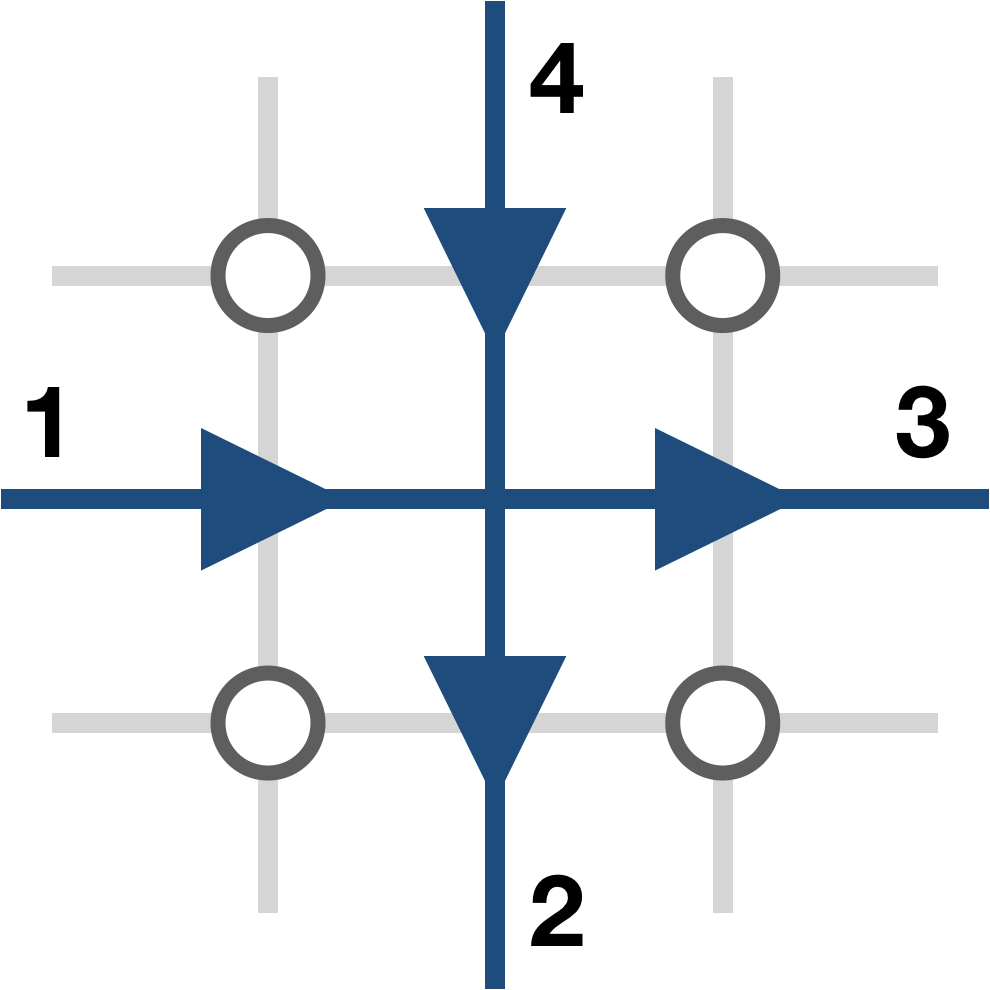
(a)

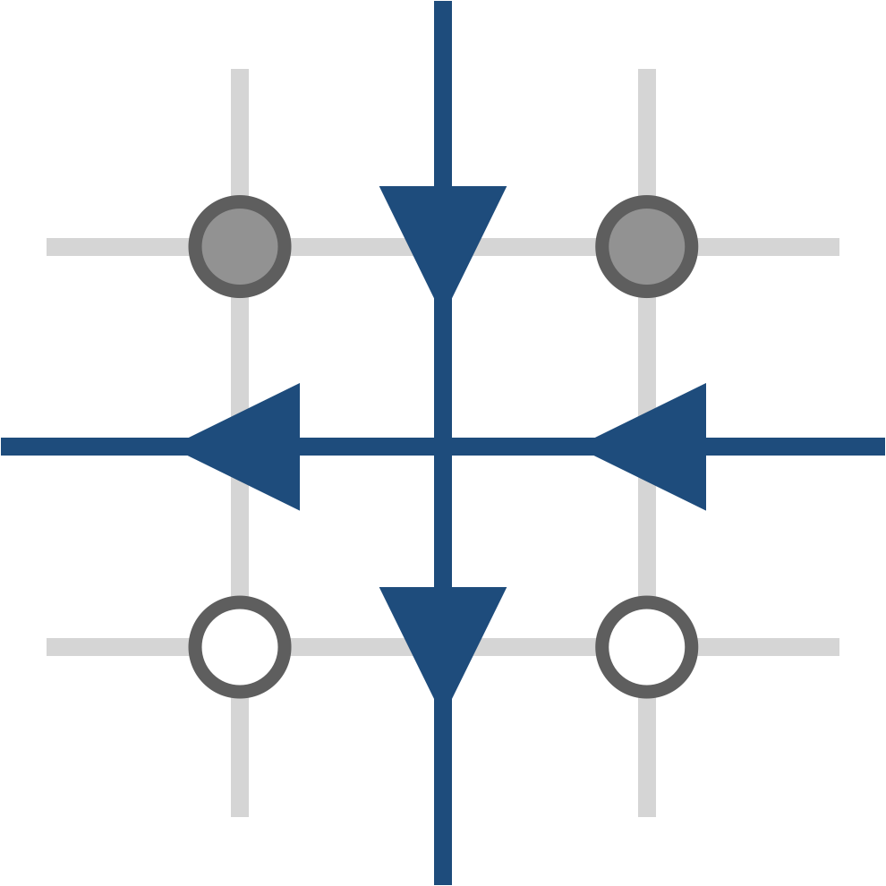
(b)

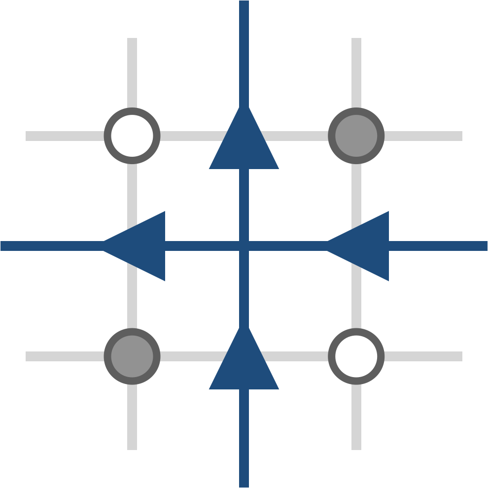
(c)

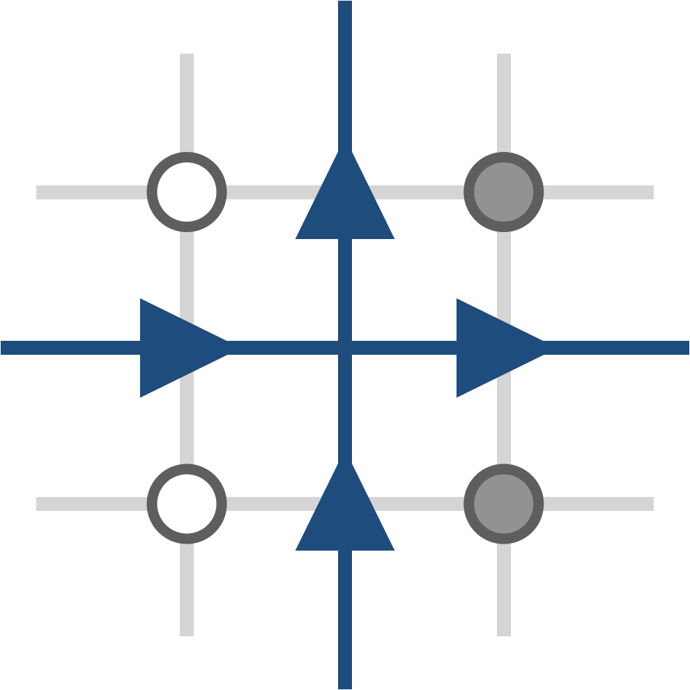
(d)

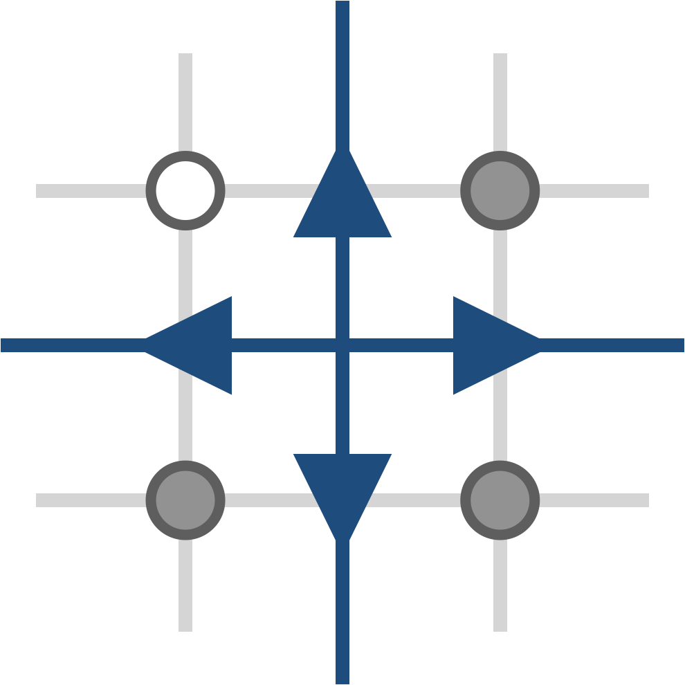
(e)

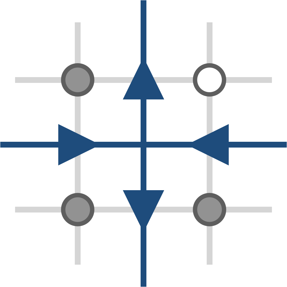
(f)

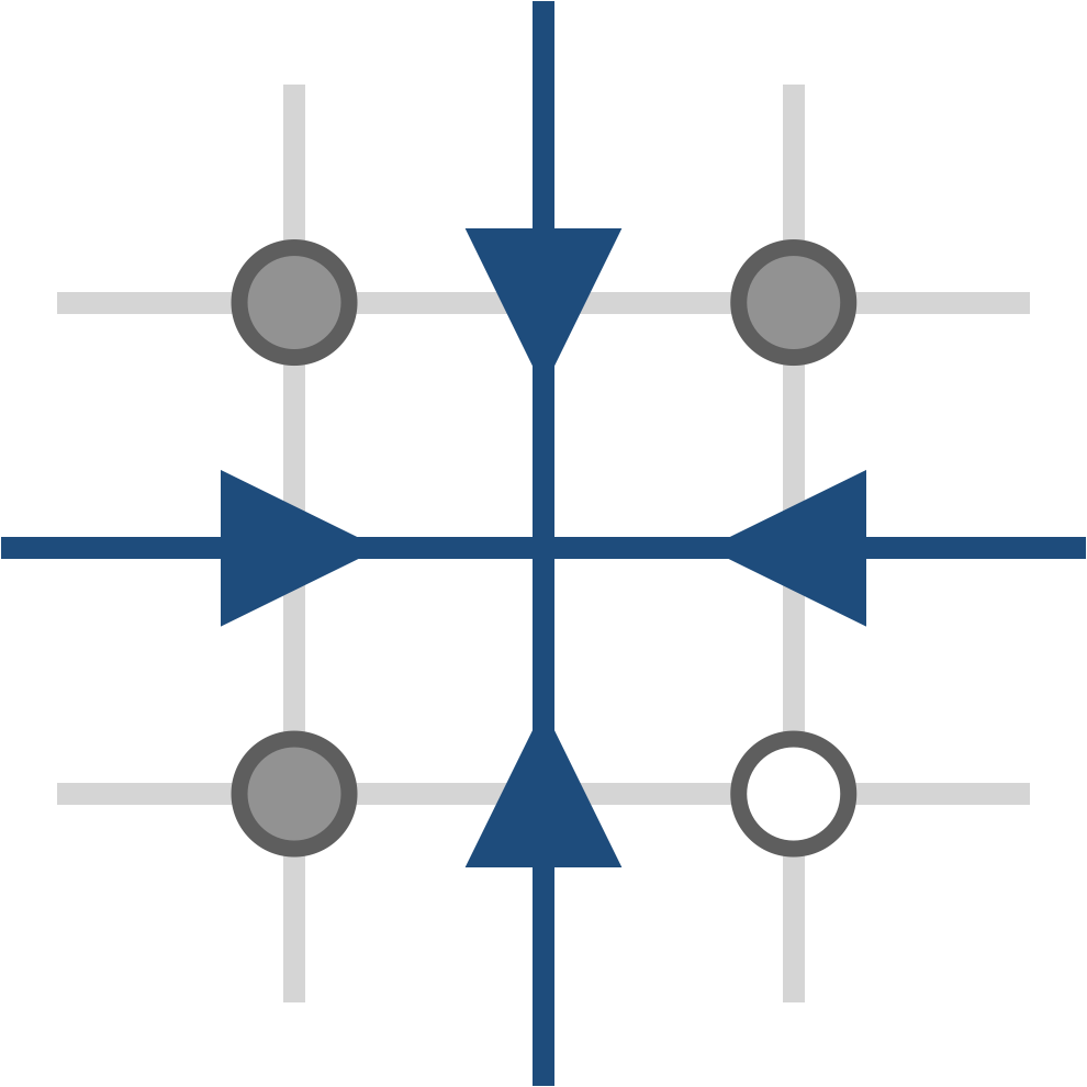
(g)

(h)

Figure 5: Mapping between the spin configurations and the vertices. (a-d): Spin configurations of ground states $\mathcal{O}_{p}=1$ correspond to vertices with zero winding number. Their energy cost is $E_{i}=-1$. (e-h): Spin configurations of Fractons $\mathcal{O}_{p}=-1$ correspond to vertices with winding number $\pm 1$. Their energy cost is $E_{i}=+1$. The correspondence is two-to-one, since flipping all spins maps to the same vertex.

The eight-vertex model is defined on the dual square lattice of the original fracton model. The mapping between the arrow and spin configurations is illustrated in Fig. 5. Each edge of the dual lattice neighbors two spins of the original lattice, at the ends of the perpendicularly intersecting edge. The arrow of the dual edge points right or down if the two spins are aligned in the same direction, and left or up otherwise. Such assignment guarantees that any four-spin configuration is mapped to one of the eight vertices listed in Fig. 4. The mapping has a global two-fold degeneracy: the vertices remain the same after flipping all spins.

The dual Hamiltonian for the eight vertex model is

$$\mathcal{H}_{\textsf{EV}}=-\frac{1}{2}\sum_{v}(\sigma_{1}\sigma_{3}+\sigma_{2}\sigma_{4}).$$ (6)

Here $v$ denotes all vertices in the dual lattice, and $\sigma_{i}$ is the value of arrows on edge $i$, defined as

$$\sigma_{i}=\begin{cases}1\qquad&\text{if it points right or down;}\\ -1\qquad&\text{if it points left or up.}\end{cases}$$ (7)

The assignment of subscripts $1,2,3,4$ around a vertex is shown in Fig. 5a. Note that this is not equivalent to a bunch of non-interacting 1-dimensional spin chains, since the constraint of eight-vertex configuration is enforced.

The vertices of winding number zero (cf. Fig.4) correspond to the ground-state spin configurations of

$$\mathcal{O}_{p}=1,$$ (8)

and have energy cost

$$E_{i}=-1\;,i=1,2,3,4.$$ (9)

Those of winding number $\pm 1$ correspond to the spin configurations of

$$\mathcal{O}_{p}=-1,$$ (10)

and have energy cost

$$E_{i}=+1\;,i=5,6,7,8\;,$$ (11)

which agree with the original fracton model (Eq. (2)). The prescription of the duality is concluded here.

The dual eight-vertex model has the advantage of illustrating various concepts of fracton models.

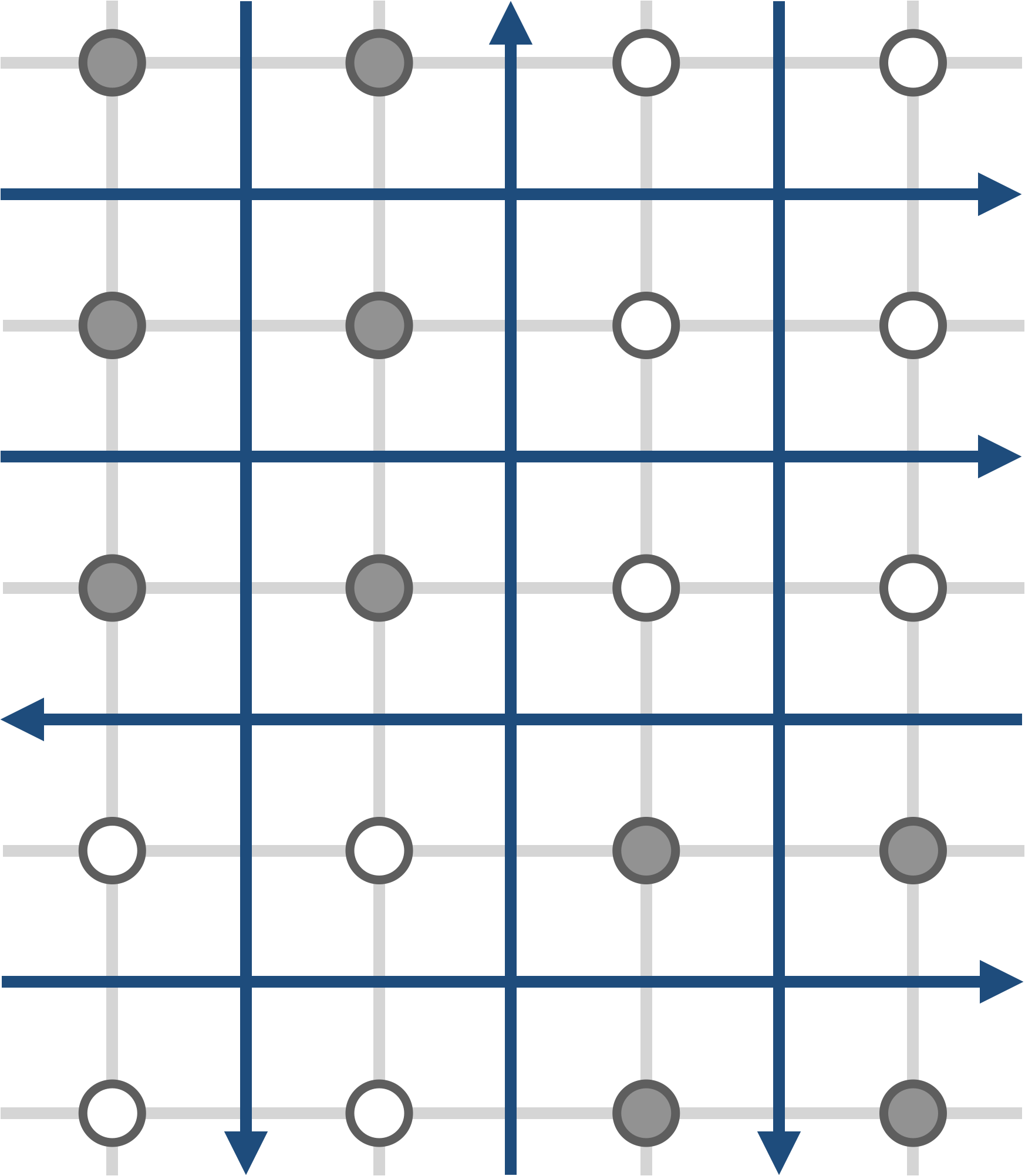
(a)

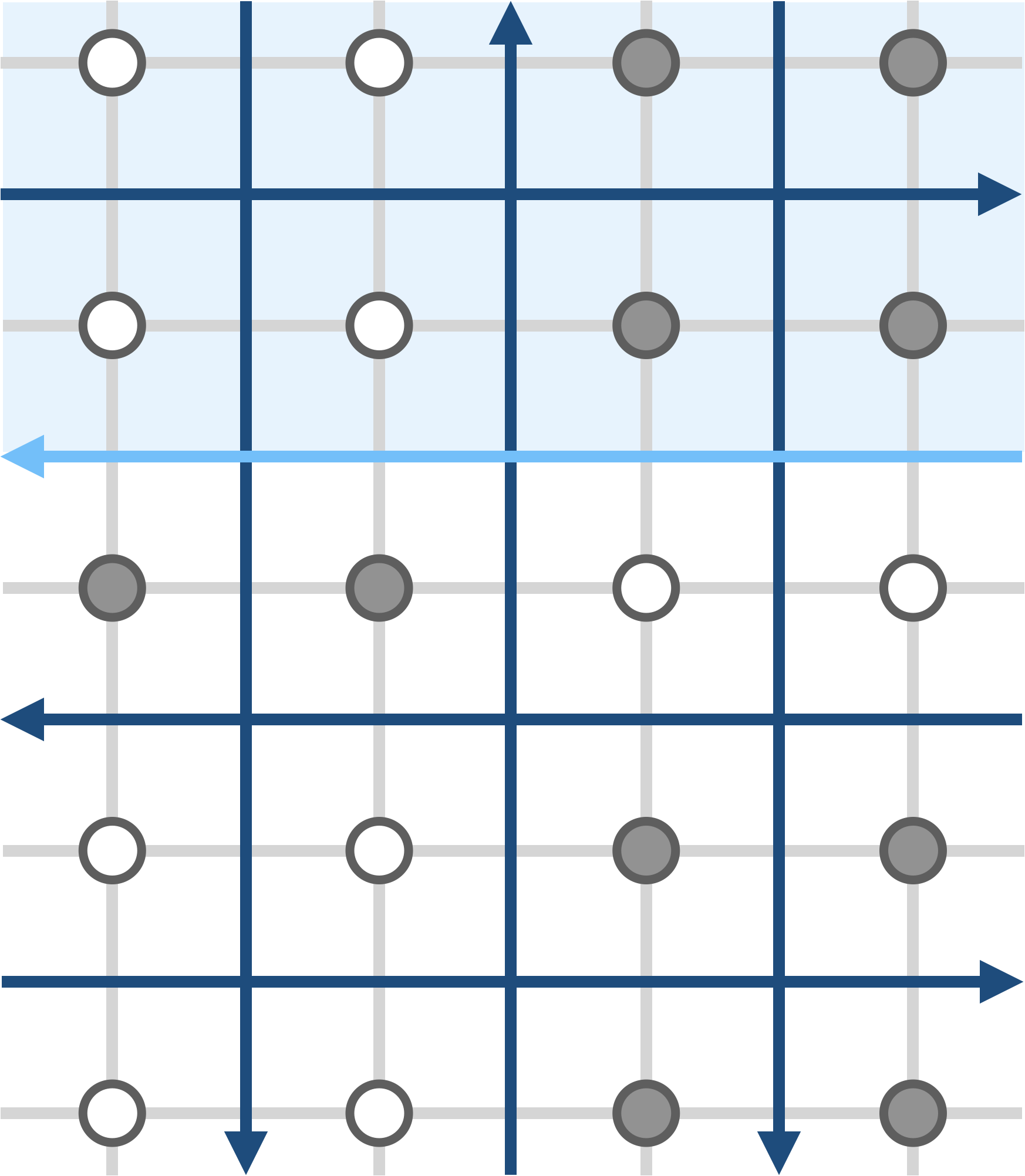
(b)

Figure 6: Ground state degeneracy in the two dual models. (a): A spin configuration of ground state, and its dual eight-vertex model state. In the eight-vertex model the ground state is such that all arrows on the same line align in the same direction. (b): Another spin configuration of ground state, obtained from (a) by flipping all spins in the light-blue shaded area. In the dual eight-vertex model it corresponds to flipping a line of arrows.

Firstly let us examine the ground state degeneracies. In the dual eight-vertex model, the ground states become very simple: all arrows on the same straight line have to align in the same direction. The action of flipping all spins on one side of a straight line corresponds to flipping the arrows of the entire line. This is illustrated in Fig. 6. The ground state ensemble is thus equivalent to a number of uncorrelated Ising spins on the boundary, which makes it apparent that its entropy is proportional to the boundary area.

Next we turn to the fracton excitations. The dual model illuminates a qualitative difference between the its effective theory — rank-two U(1) gauge theory (the traceless, scalar charged version) — and conventional U(1) gauge theory in two-dimensional space. The rank-two U(1) gauge theory accounts for the topological excitations of non-zero winding number $N_{\mathsf{w}}$ of the underlying vector field, while the conventional $U(1)$ gauge theory accounts for the non-zero net flux $C_{\mathsf{n}}$.

As one can see in Fig. 5, the fractons (vertices $5,6,7,8$ in Fig. 4), or “charge” of the rank-two electric field, are actually vertices with winding number $\pm 1$. In contrast, in the conventional electromagnetism, the “charge” is the net flux of the underlying electric field, or just the charge as we know it (vertices $5,6$).

The observation echoes the fracton-elasticity duality Pretko and Radzihovsky (2018), where the underlying vector field is the lattice distortion, and disclinations corresponds to a non-zero winding of the distortion Beekman et al. (2017).

The dual eight-vertex model is also an elegant demonstration of the subsystem symmetries and charges discussed in Vijay et al. (2016); Shirley et al. (2019a). Each Fracton vertex will introduce an $x-$ and $y-$ subsystem charge $C_{\mathsf{x}}$ and $C_{\mathsf{y}}$ on the $x-$ and $y-$direction line it is located. The charges are the flux in $x$ and $y$ listed in Fig. 4. They are related to the winding number by

$$N_{\mathsf{w}}=\frac{C_{\mathsf{x}}C_{\mathsf{y}}}{4}.$$ (12)

Two different lines have their independent charges. The total charge of each line, which can be $0$ or $\pm 2$, must be conserved by local spin flipping. Therefore a single fracton is completely localized, since moving it will change the subsystem charges. A two-fracton bound state can move in $x-$direction if they give zero charge on the $y-$direction lines. A four-fracton bound state has zero subsystem charge on any line, hence is free to move.

IV Hyperbolic Dual Eight-Vertex Model

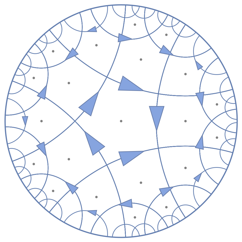
Figure 7: Dual eight-vertex model on the hyperbolic disk at $T=0$. Each geodesic carries an independent binary arrow.

The eight-vertex model dual to the hyperbolic fracton model is obtained by simply upgrading the square lattice to the $(5,4)$ tessellation of the hyperbolic disk. In the dual model, each pentagon’s edge has an associated binary arrow, and vertices are still restricted to the eight configurations in Fig. 4. Here we assign the arrow directions in the following way: We start from the obvious fracton model ground state of all spins pointing up. We then define the corresponding vertex model configuration is that (1) all arrows on the same geodesic align in the same direction; (2) the arrow on the geodesic flows clock-wise. All other vertex states are fixed following these rules.

For the ground state, all edges on the same geodesic have aligned arrows. Flipping all spins on one side of a geodesic corresponding to flipping its arrow direction. Fig. 7 shows one example of ground state eight-vertex model configurations. For fracton excitations, the concept of subsystem charges for each geodesic is also still valid.

V Bit-Thread Realization

When restricted to its ground states, the dual eight-vertex model becomes a collection of geodesics, each associated with a binary arrow. This is a simple discrete and classical realization of the bit-thread model proposed in Ref. Freedman and Headrick (2017) as a powerful conceptual tool to visualize holography.

In the bit-thread model, the elementary physical object is a divergence-free vector field in the bulk with pointwise bounded norm, referred to as the flow. Like how physicists visualize electric/magnetic fields, the flow lines can be viewed as threads. Each thread carries an independent bit of information (or two entangled qubits), and stretches from one boundary point to another. The full-fledged geometric theory of the bit-thread model is able to account for various properties of holographic entanglement entropy. For example, since the covering geodesic of boundary subregion $A$ is the narrowest bottleneck separating $A$ and its complement $A^{c}$, it sets the upper bound of the entanglement entropy between them. Following the max-flow min-cut principle Freedman and Headrick (2017), this upper bound is saturated, so that the entanglement entropy obeys the RT formula.

In the eight-vertex model at zero temperature, each geodesic is a thread or discretized flow, and carries the binary arrow as one bit of classical information. The bit threads visualize the mutual information between two subregions. It is simply counted by how many geodesics the two subregions share, as both subsystems can measure the directions of these arrows.

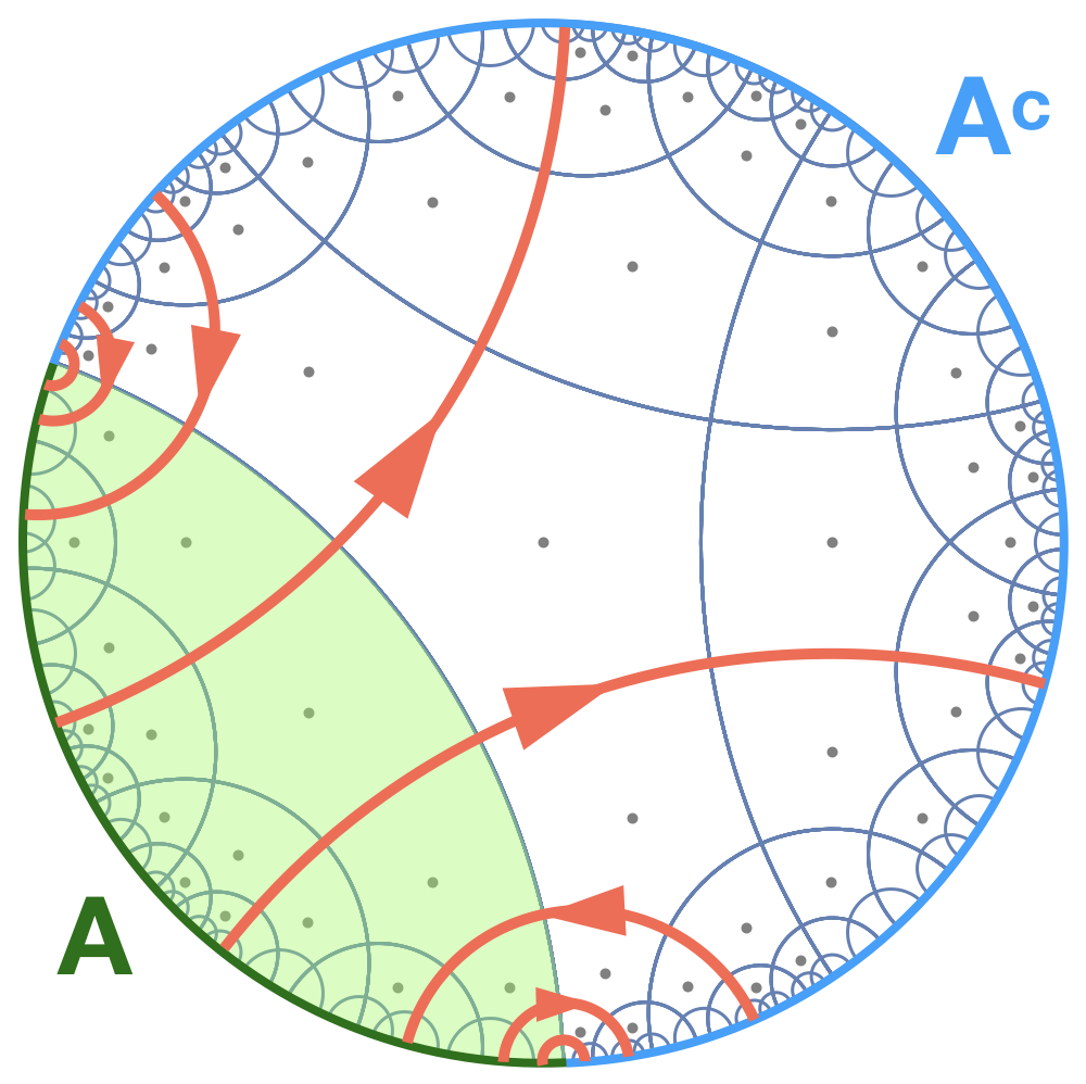
Figure 8: Bit-Thread Realization and Ryu-Takayanagi formula for mutual information. Each geodesic is a thread carrying a bit of information. The threads shared between two region (blue and green) saturates the bottleneck between them, i.e., the covering minimal surface. Hence the mutual information obeys the RT formula.

The idea of the minimal covering surface being the bottleneck is clearly represented in the eight-vertex model. As shown in Fig. 8, the geodesics highlighted in orange are the threads carrying the mutual information from boundary segment $A$ (green) to its complement $A^{c}$ (blue). It is straightforward to identify that the minimal covering surface, or the geodesic homologous to $A$, is the bottle neck of the orange region-crossing threads, which is exactly the picture described in the bit thread model.

The bit-thread model realization is simple, yet bears some non-trivial implications. We know that the rank-2 U(1) theories are linearized limit of certain gravitational theory, and the toy fracton model here is a discretized and Higgsed version of the rank-2 U(1) theories. By studying the field theory and utilizing the duality established here, it might be possible to derive the full bit-thread model from (linearized) gravity. This would be an interesting result for holographers.

We noticed a recent development yields very similar results. In Ref.Jahn et al. (2019), Jahn etc. studied the holographic tensor network in the language of majorana dimers, and discovered that the tensor networks have the same picture as we described here — entangled EPR pairs are linked by bit threads that form the hyperbolic lattice. This is a very strong indication of hidden connections between fracton models and holographic tensor networks.

VI Bulk-Boundary Isometry for Diluted Fracton Excitations

Isometry is a core issue for toy models of holography Pastawski et al. (2015); Yang et al. (2016); Hayden et al. (2016); Qi and Yang (2018). In the context of the classical fracton toy models, roughly speaking, isometry means to require that the boundary can unambiguously determine the bulk. It can be rigorously defined as :

Definition: A subset of all possible spin/vertex states is isometric, if none of its two elements have the same boundary state.

That is to say, within the chosen subset of all possible spin/vertex states,  the boundary state uniquely determines the bulk. Of course, the subset has to be a sensible choice – normally we would expect it to contain many low-energy states. For example, if it is the set of all the ground states, then isometry holds exactly.

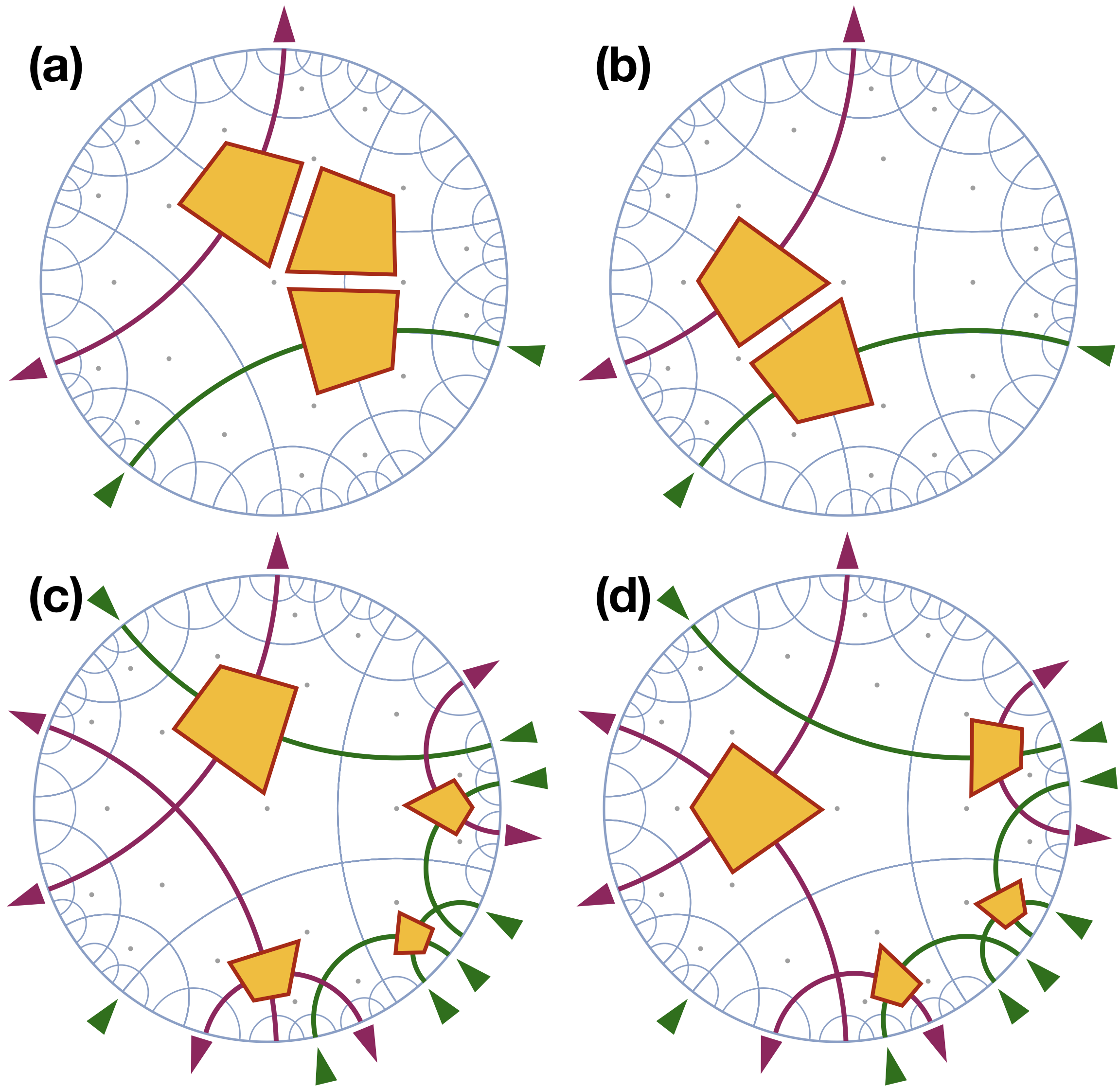
Figure 9: Two examples of isometry violation. (a, b) The dense three-fracton excited states cannot be distinguished from the two-fracton excited states from the boundary. (c, d) Two states with four-fracton excitations cannot be distinguished from the boundary.

If the subset includes certain configurations at higher energies, the isometry will eventually break down. Two examples are given in Fig. 9. This means the violation of holography, but is acceptable. Because for toy models, it is often the case that isometry (and thus holography) only holds at low energy. After all, the AdS geometry will be distorted beyond small perturbations by local high energy excitations, which is not captured by the toy models at all.

The question now becomes: how can we include more configurations at higher energy levels but maintain isometry? Or equivalently, if we include all states below a certain energy level, how much is the isometry broken?

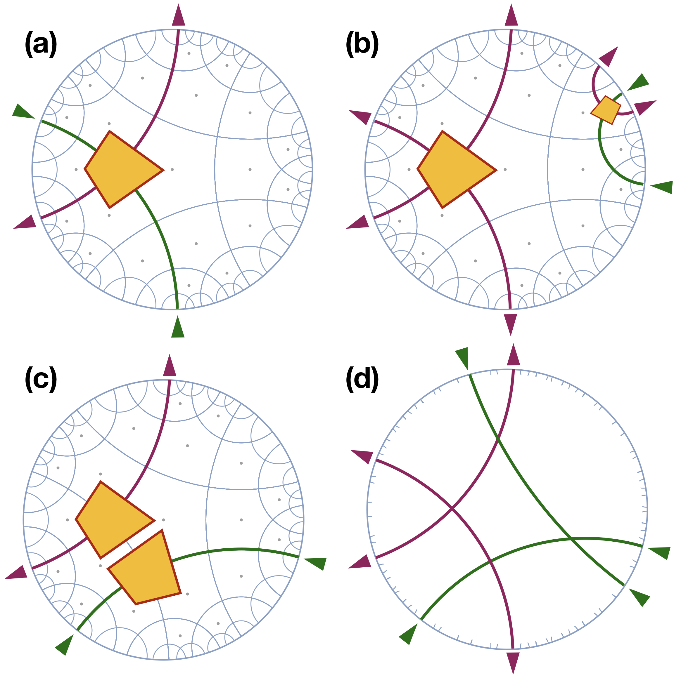
Figure 10: (a) A single fracton excitation can be reconstructed from the boundary by identifying the geodesics with non-zero subsystem charges. (b, c) Two-fracton excitations can also be reconstructed, even if they lie on the same geodesic which has zero-charge from boundary point of view. Because such geodesic can be uniquely identified. (d) Geodesics in this configuration are forbidden by the lattice geometry, which guarantees situations of (b) are always unambiguous about the locations of two fractons.

To start with, including all single fracton excited states does not break isometry. This is almost obvious, but we still analyze it in the eight-vertex picture to pave way for more complicated situations. As we discussed in Sec. III, each geodesic has its own subsystem charge. A fracton will introduce non-zero subsystem charges to the two geodesics $\gamma_{1}$ and $\gamma_{2}$ it sits on. So the subsystem charge is zero if there are zero or even number of fractons sitting on it, and $\pm 2$ if there are odd number of fractons sitting on it. In the case of a single fracton excitation, by examining the boundary arrows, we can identify $\gamma_{1}$ and $\gamma_{2}$ with $\pm 2$ charges, thus determine the location of the fracton, and the entire bulk (Fig. 10a).

All the two fracton excited states can also be included in this subset. The most-likely case is that we have four geodesics with non-zero subsystem charges, which pins down the two fractons (Fig. 10b). The hyperbolic lattice geometry guarantees us that situation like Fig. 10d will never happen, since in that case the four geodesics form a rectangle with all its corners of angle $\pi/2$. Such rectangles cannot exist in hyperbolic geometry.

The other possibility is when the two fractons sit on the same geodesic, a situation illustrated in Fig. 10c . In this case there are only two geodesics with non-zero subsystem charges. However, due to the lattice geometry, there is one and only one geodesic that intersects both, so it can be uniquely determined. Hence the two fractons’ positions can always be located.

The isometry will be broken if we further include all three-fracton excited states. Figs. 9a,b illustrate one of such examples, in which the three-fracton excited state has the same boundary as the two-fracton excited state. This can be fixed by excluding the cases when the three-fracton excitations are dense, that is, they locate around the same pentagon. Once such cases are removed from the subset, so that only the diluted three-fracton excitations are included, isometry is recovered.

The same procedure can be applied as higher-energy states are included: if by local operations a state can be turned into a lower energy one (Figs. 9a,b) or one at the same energy level (Figs. 9c,d), it should excluded in the subset. In this way we include as many lower energy states possible while maintaining isometry. To enumerate all cases is a slightly tedious task, but in principle achievable. Roughly speaking, as long as the fracton excitations are “diluted”, isometry holds. This is actually very sensible, since high energy density means distortion of the local space geometry, where the lattice model is not a good representation anymore.

Coming back to the question in the beginning of this section, at low energy levels, we can include most of the states without violating isometry. Or, if we include all states at low energy levels, the isometry is not broken too much. This is also the case of holographic tensor networks Yang et al. (2016)

An interesting side note is that the mostly-preserved isometry for low energy excitations is a consequence of the negatively-curvatured geometry. On the Euclidean lattice, isometry is completely violated starting from two fracton excitations.

VII Non-Local Black Hole Microstate Degree of Freedom

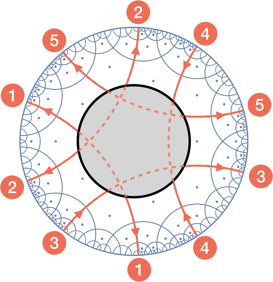
Figure 11: A black hole in the hyperbolic fracton model. The five labeled geodesics are cut into five pairs. The black hole microscopic degrees of freedom are whether each pair has aligned arrows (pair 3 here) or anti-aligned arrows (pair 1, 2, 4, 5 here).

Another concept made clear in the dual picture is the black hole microstates, which turn out to be non-locally encoded on the horizon and also on the boundary.

In Ref. Yan (2019), we used the increase of ground state entropy in the bulk to compute the black hole entropy. An equivalent definition of black hole entropy is the entropy from the microstates of the black hole Hawking (1975). In the spin picture from the hyperbolic fracton model, how to identify them is a bit obscure: the microstate dofs are not the spins next to the horizon, since they are collectively constrained by the non-local symmetry structure, and not independent from each other.

In the dual vertex model, the microstates of the black hole become clear. Let us take the black hole in Fig. 11 as an example. There are five geodesics cut open by the black hole. So attached to the horizon are ten threads, extending to the boundary.

Let us first consider the original ground states without the black hole. From the boundary point of view, they are those that each pair of threads aligned in the same direction, so that each geodesic has zero subsystem charge. We define the normalized subsystem charge

$$c_{i}=\frac{C_{i}}{2}\mod 2,$$ (13)

where the $C_{i}$ denotes the subsystem charge from the $i$-th pair of bit-threads observed from the boundary. The ground states then can be expressed collectively as states satisfying

$$(c_{1},c_{2},c_{3},c_{4},c_{5})=(0,0,0,0,0).$$ (14)

After introducing the black hole, the two bit-threads in each pair become independent. For the boundary, that means the normalized subsystem charges for these pairs can be

$$c_{i}=1,\ \text{or }0.$$ (15)

The different black hole microstates correspond to different arrays $(c_{1},c_{2},c_{3},c_{4},c_{5})$. That is, the dofs living on the horizon are whether each pair of threads is aligned or not. Or in more mathematical terms, the microstates are all the ground states quotient the subsystem symmetries from the no-black-hole bulk. Here we emphasis that the single bit-threads should not be viewed as the dofs individually. This is a critical to identify the correct black hole microstates: different states connected by subsystem symmetries should not be counted, since they are already included in the entropy contribution of ground states without black holes. This is also reason we use the normalized subsystem charge $c_{i}$ instead of the original $C_{i}$: to guarantee that the microstate is invariant under subsystem symmetries.

A sanity check is to consider the “entanglement entropy” as half the classical mutual information between the black hole and the AdS boundary. As mentioned, the mutual information is counted by the number of threads ending on the horizon on one side and the AdS boundary on the other side. So the entanglement entropy is counted by this number divided by two, i.e., each pair of thread counts as one dof. This is consistent with the microstate dof counting.

One interesting implication of the result is that the black hole dofs are encoded non-locally. A single thread of a pair only gives some information of $C_{i}$ but no information of $c_{i}$ at all. Only when both bit-threads are known can we recover the value of $c_{i}$. Thus the black hole microstate information is non-locally encoded on its horizon and also the AdS boundary.

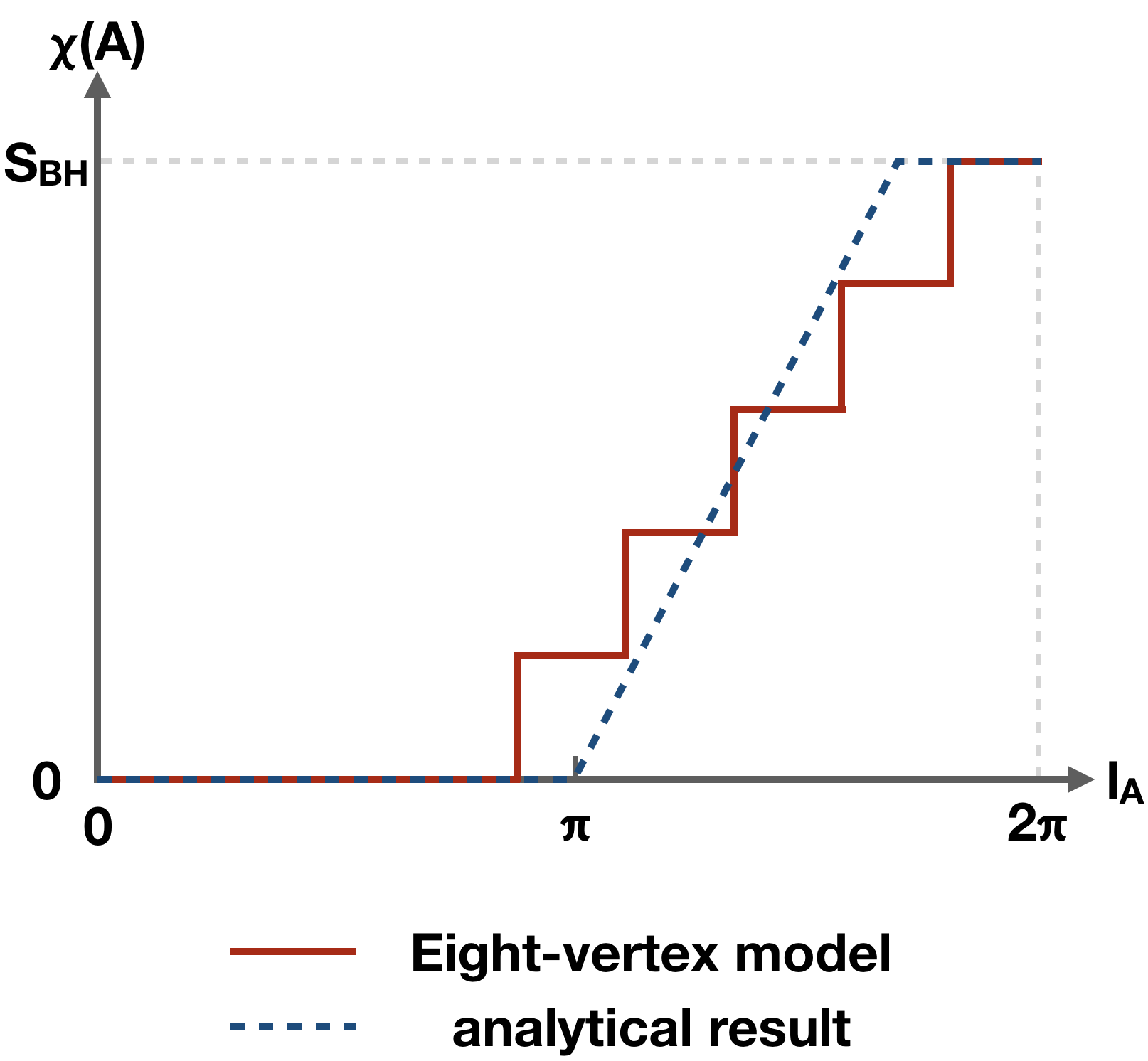
Figure 12: Black hole microstate information for observer covering a subregion of the boundary. Red line: in the eight-vertex model, the observer starts to have black hole microstate information when covering a pair of geodesics cut open by the black hole (Fig. 11). Such information is zero until the observer reaches about half the boundary size, and gradually grows till the observer almost covers the entire boundary. Blue line: analytical calculation of the Holevo information measuring the microstate distinguishability as a function of the boundary subregion area measurable to the observer in Ref. Bao and Ooguri (2017). Even though the black hole in the eight-vertex model is very naively defined, the black hole information recovery behavior looks similar to the analytical results.

Such conclusion agrees with the analysis in Ref. Bao and Ooguri (2017), where the authors discussed how much of the AdS boundary subregion needs to be measured to distinguish black hole microstates.

In our bit-thread model, as the observer starts to expand the observed subregion on the boundary, he/she will know the arrow directions of more threads. But any pair of thread heads from the black hole is separated by a macroscopic distance, so starting from zero up to a finite subregion, the observer cannot infer any information about the black hole microstate. As the first pair of cut-open threads is included in the observed subregion, the observer begins to have some information of the black hole microstates, and the amount of information grows approximately linearly as the subregion expands. Finally when almost covering the full boundary, the observer can obtain all the information of the black hole microstate.

In Fig. 12, we plot the black hole microstate information as a function of the observed subregion from the eight-vertex model, as well as the analytical result obtained in Ref. Bao and Ooguri (2017). The behaviors of the two curves qualitatively agree, in terms of the zero information segment in the beginning, the linear growth in the middle and the final saturation.

VIII Outlook

In this work we discussed in detail the implications of the dual eight-vertex model equivalent to the original hyperbolic fracton model. Despite the equivalence, it advances our understanding by providing a much clearer picture of a few aspects of its physics.

The hyperbolic eight-vertex model becomes a discrete bit-thread model at zero temperature. This explains why the fracton model has the holographic properties demonstrated before. It is also significant that we have another concrete, sophisticated holographic model – the bit-thread model – as a reference frame to evaluate the similarity between fracton models and the informational-aspects of holography. It is a very useful guideline to construct improved holographic fracton models. For example, fracton bit-threads being discrete is a major obstacle for holography at higher order (for disconnected boundary components), or below the AdS scale (i.e., for regions smaller than the pentagon). So an improved version should tackle such problems.

The connection between the fracton model and bit-threads also implies that it might be possible to establish a concrete duality between linearized gravity (or theories with linearized diffeomorphism-like gauge symmetry) and the full-fledged bit-thread model. It has been pointed out that rank-2 U(1) gauge theory, the underlying effective theory of the hyperbolic fracton model (with Higgs mechanism), is actually the linearized limit of certain gravitational theory. This also gives us some confidence in constructing more sophisticated holographic fracton models to mimic gravity better.

At finite temperature, utilizing the bit-thread picture and subsystem charges, one can establish isometry for a subset of low energy states, and identify the non-locally encoded black hole microscopic dofs. It is intriguing to ask what will these subsystem charges become when we work on the continuous field theory, or what is their analogy in gravity.

To explore the relationship between gravity and fracton states can be a meaningful program for condensed matter physics. A lot is known on how topological orders are described by gauge theories, but not much on what kind of (beyond) topological order can arise from gravitational-like theories. Certain fracton states seem to be such examples Pretko (2017c); Gromov (2019); Slagle et al. (2019), but the whole picture is vastly unexplored.

If we could discover more gravity-like many-body systems, they may also help us establish links between gravity and various other toy models of holography, including the holographic tensor networks and the bit-thread model. This work already serves as a primitive example of the latter case. It is also attractive to mimic gravity in a laboratory using fracton states, after we understand their relations better.

References

- Yan (2019) H. Yan, Phys. Rev. B 99, 155126 (2019).
- Chamon (2005) C. Chamon, Phys. Rev. Lett. 94, 040402 (2005).
- Yoshida (2013) B. Yoshida, Phys. Rev. B 88, 125122 (2013).
- Bravyi et al. (2011) S. Bravyi, B. Leemhuis, and B. M. Terhal, Annals of Physics 326, 839 (2011).
- Haah (2011) J. Haah, Phys. Rev. A 83, 042330 (2011).
- Vijay et al. (2015) S. Vijay, J. Haah, and L. Fu, Phys. Rev. B 92, 235136 (2015).
- Vijay et al. (2016) S. Vijay, J. Haah, and L. Fu, Phys. Rev. B 94, 235157 (2016).
- Pretko (2017a) M. Pretko, Phys. Rev. B 96, 035119 (2017a).
- Pretko (2017b) M. Pretko, Phys. Rev. B 95, 115139 (2017b).
- Nandkishore and Hermele (2019) R. M. Nandkishore and M. Hermele, Annual Review of Condensed Matter Physics 10, 295 (2019), https://doi.org/10.1146/annurev-conmatphys-031218-013604 .
- Shirley et al. (2018) W. Shirley, K. Slagle, Z. Wang, and X. Chen, Phys. Rev. X 8, 031051 (2018), arXiv:1712.05892 .
- Slagle et al. (2019) K. Slagle, D. Aasen, and D. Williamson, SciPost Phys. 6, 43 (2019).
- Tian et al. (2018) K. T. Tian, E. Samperton, and Z. Wang, arXiv e-prints , arXiv:1812.02101 (2018), arXiv:1812.02101 [quant-ph] .
- You (2019) Y. You, arXiv e-prints , arXiv:1901.07163 (2019), arXiv:1901.07163 [cond-mat.str-el] .
- Song et al. (2019) H. Song, A. Prem, S.-J. Huang, and M. A. Martin-Delgado, Phys. Rev. B 99, 155118 (2019).
- You et al. (2018) Y. You, T. Devakul, F. J. Burnell, and S. L. Sondhi, Phys. Rev. B 98, 035112 (2018).
- Slagle and Kim (2017) K. Slagle and Y. B. Kim, Phys. Rev. B 96, 165106 (2017).
- Hsieh and Halász (2017) T. H. Hsieh and G. B. Halász, Phys. Rev. B 96, 165105 (2017).
- Halász et al. (2017) G. B. Halász, T. H. Hsieh, and L. Balents, Phys. Rev. Lett. 119, 257202 (2017).
- Ma et al. (2017) H. Ma, E. Lake, X. Chen, and M. Hermele, Phys. Rev. B 95, 245126 (2017).
- You and von Oppen (2018) Y. You and F. von Oppen, arXiv e-prints , arXiv:1812.06091 (2018), arXiv:1812.06091 [cond-mat.str-el] .
- Yan et al. (2019) H. Yan, O. Benton, L. D. C. Jaubert, and N. Shannon, arXiv e-prints , arXiv:1902.10934 (2019), arXiv:1902.10934 [cond-mat.str-el] .
- Benton et al. (2016) O. Benton, L. D. C. Jaubert, H. Yan, and N. Shannon, Nat. Commun. 7, 11572 (2016).
- Shirley et al. (2018) W. Shirley, K. Slagle, and X. Chen, ArXiv e-prints (2018), arXiv:1803.10426 [cond-mat.str-el] .
- Pai and Hermele (2019) S. Pai and M. Hermele, arXiv e-prints , arXiv:1903.11625 (2019), arXiv:1903.11625 [cond-mat.str-el] .
- Gromov (2018) A. Gromov, arXiv e-prints , arXiv:1812.05104 (2018), arXiv:1812.05104 [cond-mat.str-el] .
- Shirley et al. (2019a) W. Shirley, K. Slagle, and X. Chen, SciPost Phys. 6, 41 (2019a).
- Schmitz et al. (2018) A. T. Schmitz, H. Ma, R. M. Nandkishore, and S. A. Parameswaran, Phys. Rev. B 97, 134426 (2018).
- Kubica and Yoshida (2018) A. Kubica and B. Yoshida, ArXiv e-prints (2018), arXiv:1805.01836 [quant-ph] .
- He et al. (2018) H. He, Y. Zheng, B. A. Bernevig, and N. Regnault, Phys. Rev. B 97, 125102 (2018).
- Ma et al. (2018) H. Ma, A. T. Schmitz, S. A. Parameswaran, M. Hermele, and R. M. Nandkishore, Phys. Rev. B 97, 125101 (2018).
- Schmitz (2018) A. T. Schmitz, arXiv e-prints , arXiv:1809.10151 (2018), arXiv:1809.10151 [quant-ph] .
- Schmitz et al. (2019) A. T. Schmitz, S.-J. Huang, and A. Prem, arXiv e-prints , arXiv:1901.10486 (2019), arXiv:1901.10486 [quant-ph] .
- Pai et al. (2019) S. Pai, M. Pretko, and R. M. Nandkishore, Phys. Rev. X 9, 021003 (2019).
- Shirley et al. (2019b) W. Shirley, K. Slagle, and X. Chen, SciPost Phys. 6, 15 (2019b).
- Pretko (2017c) M. Pretko, Phys. Rev. D 96, 024051 (2017c).
- Pretko and Radzihovsky (2018) M. Pretko and L. Radzihovsky, Physical Review Letters 120, 195301 (2018), arXiv:1711.11044 [cond-mat.str-el] .
- Pai and Pretko (2018) S. Pai and M. Pretko, Phys. Rev. B 97, 235102 (2018).
- Pretko and Radzihovsky (2018) M. Pretko and L. Radzihovsky, Phys. Rev. Lett. 121, 235301 (2018).
- Gromov (2019) A. Gromov, Phys. Rev. Lett. 122, 076403 (2019).
- Xu (2006) C. Xu, Phys. Rev. B 74, 224433 (2006).
- Rasmussen et al. (2016) A. Rasmussen, Y.-Z. You, and C. Xu, ArXiv e-prints (2016), arXiv:1601.08235 [cond-mat.str-el] .
- Slagle and Kim (2017) K. Slagle and Y. B. Kim, ArXiv e-prints (2017), arXiv:1712.04511 [cond-mat.str-el] .
- Prem et al. (2018) A. Prem, S.-J. Huang, H. Song, and M. Hermele, arXiv e-prints , arXiv:1806.04687 (2018), arXiv:1806.04687 [cond-mat.str-el] .
- You et al. (2018) Y. You, T. Devakul, F. J. Burnell, and S. L. Sondhi, arXiv e-prints , arXiv:1805.09800 (2018), arXiv:1805.09800 [cond-mat.str-el] .
- Bulmash and Barkeshli (2018) D. Bulmash and M. Barkeshli, Phys. Rev. B 97, 235112 (2018).
- Ma et al. (2018) H. Ma, M. Hermele, and X. Chen, Phys. Rev. B 98, 035111 (2018), arXiv:1802.10108 [cond-mat.str-el] .
- Slagle et al. (2018) K. Slagle, A. Prem, and M. Pretko, arXiv e-prints , arXiv:1807.00827 (2018), arXiv:1807.00827 [cond-mat.str-el] .
- Shirley et al. (2018) W. Shirley, K. Slagle, Z. Wang, and X. Chen, Phys. Rev. X 8, 031051 (2018).
- Devakul et al. (2019) T. Devakul, Y. You, F. J. Burnell, and S. L. Sondhi, SciPost Phys. 6, 7 (2019).
- Hooft (1974) G. Hooft, Nucl. Phys. B 72, 461 (1974).
- Susskind (1995) L. Susskind, J. Math. Phys. 36, 6377 (1995).
- Maldacena (1999) J. Maldacena, Int. J. Theor. Phys. 38, 1113 (1999).
- Witten (1998) E. Witten, Adv. Theor. Math. Phys. 2, 253 (1998).
- Gubser et al. (1998) S. S. Gubser, I. R. Klebanov, and A. M. Polyakov, Phys. Lett. B 428, 105 (1998), hep-th/9802109 .
- Aharony et al. (2000) O. Aharony, S. S. Gubser, J. Maldacena, H. Ooguri, and Y. Oz, Phys. Rep. 323, 183 (2000).
- Aharony et al. (2008) O. Aharony, O. Bergman, D. L. Jafferis, and J. Maldacena, JHEP 2008, 091 (2008).
- Klebanov and Polyakov (2002) I. Klebanov and A. Polyakov, Phys. Lett. B 550, 213 (2002).
- Hawking (2005) S. W. Hawking, Phys. Rev. D 72, 084013 (2005).
- Guica et al. (2009) M. Guica, T. Hartman, W. Song, and A. Strominger, Phys. Rev. D 80, 124008 (2009).
- Hartnoll et al. (2016) S. Hartnoll, A. Lucas, and S. Sachdev, Holographic quantum matter (The MIT Press, 2016) p. 390, arXiv:1612.07324 .
- Pires (2014) A. S. T. Pires, AdS/CFT Correspondence in Condensed Matter, 2053-2571 (Morgan & Claypool Publishers, 2014).
- Zaanen et al. (2015) J. Zaanen, Y. Liu, Y.-W. Sun, and K. Schalm, Holographic Duality in Condensed Matter Physics (Cambridge University Press, 2015).
- Nastase (2017) H. Nastase, String Theory Methods for Condensed Matter Physics (Cambridge University Press, 2017).
- Qi (2013) X.-L. Qi, ArXiv e-prints (2013), arXiv:1309.6282 [hep-th] .
- Gu et al. (2016) Y. Gu, C. H. Lee, X. Wen, G. Y. Cho, S. Ryu, and X.-L. Qi, Phys. Rev. B 94, 125107 (2016).
- Lee and Qi (2016) C. H. Lee and X.-L. Qi, Phys. Rev. B 93, 035112 (2016).
- Ryu and Takayanagi (2006a) S. Ryu and T. Takayanagi, JHEP 2006, 045 (2006a).
- Ryu and Takayanagi (2006b) S. Ryu and T. Takayanagi, Phys. Rev. Lett. 96, 181602 (2006b).
- Van Raamsdonk (2009) M. Van Raamsdonk, arXiv e-prints , arXiv:0907.2939 (2009), arXiv:0907.2939 [hep-th] .
- Swingle (2012) B. Swingle, Phys. Rev. D 86, 065007 (2012).
- Pastawski et al. (2015) F. Pastawski, B. Yoshida, D. Harlow, and J. Preskill, JHEP 2015, 149 (2015).
- Almheiri et al. (2015) A. Almheiri, X. Dong, and D. Harlow, JHEP 2015, 163 (2015).
- Yang et al. (2016) Z. Yang, P. Hayden, and X.-L. Qi, JHEP 2016 (2016), 10.1007/jhep01(2016)175.
- Hayden et al. (2016) P. Hayden, S. Nezami, X.-L. Qi, N. Thomas, M. Walter, and Z. Yang, JHEP 2016, 9 (2016).
- Qi and Yang (2018) X.-L. Qi and Z. Yang, ArXiv e-prints (2018), arXiv:1801.05289 [hep-th] .
- Harlow (2017) D. Harlow, Communications in Mathematical Physics 354, 865 (2017), arXiv:1607.03901 [hep-th] .
- Freedman and Headrick (2017) M. Freedman and M. Headrick, Communications in Mathematical Physics 352, 407 (2017), arXiv:1604.00354 [hep-th] .
- Cui et al. (2018) S. X. Cui, P. Hayden, T. He, M. Headrick, B. Stoica, and M. Walter, ArXiv e-prints (2018), arXiv:1808.05234 [hep-th] .
- Harper et al. (2018) J. Harper, M. Headrick, and A. Rolph, ArXiv e-prints (2018), arXiv:1807.04294 [hep-th] .
- Headrick and Hubeny (2018) M. Headrick and V. E. Hubeny, Classical and Quantum Gravity 35, 105012 (2018), arXiv:1710.09516 [hep-th] .
- Chen et al. (2018) C.-B. Chen, F.-W. Shu, and M.-H. Wu, ArXiv e-prints (2018), arXiv:1804.00441 [hep-th] .
- Bao and Ooguri (2017) N. Bao and H. Ooguri, Phys. Rev. D 96, 066017 (2017), arXiv:1705.07943 [hep-th] .
- Hawking (1975) S. W. Hawking, Commun. Math. Phys. 43, 199 (1975).
- Sutherland (1970) B. Sutherland, Journal of Mathematical Physics 11, 3183 (1970), https://doi.org/10.1063/1.1665111 .
- Fan and Wu (1970) C. Fan and F. Y. Wu, Phys. Rev. B 2, 723 (1970).
- Baxter (1971) R. J. Baxter, Physical Review Letters 26, 832 (1971).
- Kadanoff and Wegner (1971) L. P. Kadanoff and F. J. Wegner, Phys. Rev. B 4, 3989 (1971).
- Baxter (2007) R. Baxter, Exactly Solved Models in Statistical Mechanics, Dover books on physics (Dover Publications, 2007).
- Beekman et al. (2017) A. J. Beekman, J. Nissinen, K. Wu, K. Liu, R.-J. Slager, Z. Nussinov, V. Cvetkovic, and J. Zaanen, Physics Reports 683, 1 (2017), dual gauge field theory of quantum liquid crystals in two dimensions.
- Jahn et al. (2019) A. Jahn, M. Gluza, F. Pastawski, and J. Eisert, arXiv e-prints , arXiv:1905.03268 (2019), arXiv:1905.03268 [hep-th] .