Abstract

Using machine learning in high-stakes applications often requires predictions to be accompanied by explanations comprehensible to the domain user, who has ultimate responsibility for decisions and outcomes. Recently, a new framework for providing explanations, called TED Hind et al. (2019), has been proposed to provide meaningful explanations for predictions. This framework augments training data to include explanations elicited from domain users, in addition to features and labels. This approach ensures that explanations for predictions are tailored to the complexity expectations and domain knowledge of the consumer.

In this paper, we build on this foundational work, by exploring more sophisticated instantiations of the TED framework and empirically evaluate their effectiveness in two diverse domains, chemical odor and skin cancer prediction. Results demonstrate that meaningful explanations can be reliably taught to machine learning algorithms, and in some cases, improving modeling accuracy.

1 Introduction

New regulations call for automated decision making systems to provide “meaningful information” on the logic used to reach conclusions (Goodman & Flaxman, 2016; Wachter et al., 2017; Selbst & Powles, 2017). Selbst & Powles (2017) interpret the concept of “meaningful information” as information that should be understandable to the audience (potentially individuals who lack specific expertise), is actionable, and is flexible enough to support various technical approaches.

Recently, Hind et al. (2019) introduced a new framework, called TED (Teaching Explanations for Decisions), for providing meaningful explanations for machine learning predictions. The framework requires the training dataset to include an explanation ($E$), along with the features ($X$) and target label ($Y$). A model is learned from this training set so that predictions include a label and an explanation, both of which are from the set of possible labels ($Y$) and explanations ($E$) that are provided in the training data.

This approach has several advantages. The explanations provided should meet the complexity capability and domain knowledge of the target user because they are providing the training explanations. The explanations should be as accurate as the underlying predictions. The framework is general in that it can be applied to any supervised machine learning algorithm.

In addition to describing the framework and other advantages, Hind et al. (2019) also describe a simple instantiation of the framework, based on the Cartesian product, that combines the $Y$ label and $E$ explanation to form a new training dataset ($X$, $YE$), which is then fed into any machine learning algorithm. The resulting model will produce predictions ($YE$) that can be decomposed to the $Y$ and $E$ component. This instantiation is evaluated on two synthetic datasets for playing tic-tac-toe and loan repayment. Their results show “(1) To the extent that user explanations follow simple logic, very high explanation accuracy can be achieved; (2) Accuracy in predicting $Y$ not only does not suffer but actually improves.”

In this work, we explore more sophisticated instantiations of the TED framework that leverage training explanations to improve the accuracy of prediction as well as the generation of explanations. Specifically, we explore bringing together the labels and explanations in a multi-task setting, as well as building upon the tradition of similarity metrics, case-based reasoning and content-based retrieval.

Existing approaches that only have access to features and labels are unable to find meaningful similarities. However, with the advantage of having training features, labels, and explanations, we propose to learn feature embeddings guided by labels and explanations. This allows us to infer explanations for new data using nearest neighbor approaches. We present a new objective function to learn an embedding to optimize $k$-nearest neighbor ($k$NN) search for both prediction accuracy as well as holistic human relevancy to enforce that returned neighbors present meaningful information. The proposed embedding approach is easily portable to a diverse set of label and explanation spaces because it only requires a notion of similarity between examples in these spaces. Since any predicted explanation or label is obtained from a simple combination of training examples, complexity and domain match is achieved with no further effort. We also demonstrate the multi-task instantiation wherein labels and explanations are predicted together from features. In contrast to the embedding approach, we need to change the structure of the ML model for this method due to the modality and type of the label and explanation space.

We demonstrate the proposed paradigm using the two instantiations on publicly-available olfactory pleasantness dataset (Keller et al., 2017) and melanoma classification dataset (Codella et al., 2018a). Teaching explanations requires a training set that contains explanations. Since such datasets are not readily available, we use the attributes given with the pleasantness dataset in a unique way: as collections of meaningful explanations. For the melanoma classification dataset, we will use the groupings given by human users described in Codella et al. (2018b) as the explanations.

The main contributions of this work are:

• Instantations and evaluation of several candidate TED approaches, some that learn efficient embeddings that can be used to infer labels and explanations for novel data, and some that use multi-task learning to predict labels and explanations.

• Evaluation on disparate datasets with diverse label and explanation spaces demonstrating the efficacy of the paradigm.

2 Related Work

Prior work in providing explanations can be partitioned into several areas:

1. Making existing or enhanced models interpretable, i.e. to provide a precise description of how the model determined its decision (e.g., Ribeiro et al. (2016); Montavon et al. (2017); Lundberg & Lee (2017)).

2. Creating a simpler-to-understand model, such as a small number of logical expressions, that mostly matches the decisions of the deployed model (e.g., Bastani et al. (2018); Caruana et al. (2015)), or directly training a simple-to-understand model from the data (e.g., Dash et al. (2018); Wang et al. (2017); Cohen (1995); Breiman (2017)).

3. Leveraging “rationales”, “explanations”, “attributes”, or other “privileged information” in the training data to help improve the accuracy of the algorithms (e.g., Sun & DeJong (2005); Zaidan & Eisner (2008); Donahue & Grauman (2011); Peng et al. (2016)).

4. Work in the natural language processing and computer vision domains that generate rationales/explanations derived from input text (e.g., Lei et al. (2016); Ainur et al. (2010); Hendricks et al. (2016)).

5. Content-based retrieval methods that provide explanations as evidence employed for a prediction, i.e. $k$-nearest neighbor classification and regression (e.g., Wan et al. (2014); Jimenez-del-Toro et al. (2015); Li et al. (2018); Sun et al. (2012)).

The first two groups attempt to precisely describe how a machine learning decision was made, which is particularly relevant for AI system builders. This insight can be used to improve the AI system and may serve as the seeds for an explanation to a non-AI expert. However, work still remains to determine if these seeds are sufficient to satisfy the needs of a non-AI expert. In particular, when the underlying features are not human comprehensible, these approaches are inadequate for providing human consumable explanations.

The third group, like this work, leverages additional information (explanations) in the training data, but with different goals. The third group uses the explanations to create a more accurate model; the TED framework leverages the explanations to teach how to generate explanations for new predictions.

The fourth group seeks to generate textual explanations with predictions. For text classification, this involves selecting the minimal necessary content from a text body that is sufficient to trigger the classification. For computer vision (Hendricks et al., 2016), this involves utilizing textual captions to automatically generate new textual captions of images that are both descriptive as well as discriminative. While serving to enrich an understanding of the predictions, these systems do not necessarily facilitate an improved ability for a human user to understand system failures.

The fifth group creates explanations in the form of decision evidence: using some feature embedding to perform k-nearest neighbor search, using those k neighbors to make a prediction, and demonstrating to the user the nearest neighbors and any relevant information regarding them. Although this approach is fairly straightforward and holds a great deal of promise, it has historically suffered from the issue of the semantic gap: distance metrics in the realm of the feature embeddings do not necessarily yield neighbors that are relevant for prediction. More recently, deep feature embeddings, optimized for generating predictions, have made significant advances in reducing the semantic gap. However, there still remains a “meaning gap” — although systems have gotten good at returning neighbors with the same label as a query, they do not necessarily return neighbors that agree with any holistic human measures of similarity. As a result, users are not necessarily inclined to trust system predictions.

Doshi-Velez et al. (2017) discuss the societal, moral, and legal expectations of AI explanations, provide guidelines for the content of an explanation, and recommend that explanations of AI systems be held to a similar standard as humans. Our approach is compatible with their view. Biran & Cotton (2017) provide an excellent overview and taxonomy of explanations and justifications in machine learning.

Miller (2017) and Miller et al. (2017) argue that explainable AI solutions need to meet the needs of the users, an area that has been well studied in philosophy, psychology, and cognitive science. They provides a brief survey of the most relevant work in these fields to the area of explainable AI. They, along with Doshi-Velez & Kim (2017), call for more rigor in this area.

3 Methods

The primary motivation of the TED paradigm is to provide meaningful explanations to consumers by leveraging the consumers’ knowledge of what will be meaningful to them. Section 3.1 formally describes the problem space that defines the TED approach.

This paper focuses on instantiations of the TED approach that leverages the explanations to improve model prediction and possibly explanation accuracy. Section 3.2 takes this approach to learn feature embeddings and explanation embeddings in a joint and aligned way to permit neighbor-based explanation prediction. It presents a new objective function to learn an embedding to optimize $k$NN search for both prediction accuracy as well as holistic human relevancy to enforce that returned neighbors present meaningful information. We also discuss multi-task learning in the label and explanation space as another instantiation of the TED approach, that we will use for comparisons.

3.1 Problem Description

Let $X\times Y$ denote the input-output space, with $p(x,y)$ denoting the joint distribution over this space, where $(x,y)\in X\times Y$. Then typically, in supervised learning one wants to estimate $p(y|x)$.

In our setting, we have a triple $X\times Y\times E$ that denotes the input space, output space, and explanation space, respectively. We then assume that we have a joint distribution $p(x,y,e)$ over this space, where $(x,y,e)\in X\times Y\times E$. In this setting we want to estimate $p(y,e|x)=p(y|x)p(e|y,x)$. Thus, we not only want to predict the labels $y$, but also the corresponding explanations $e$ for the specific $x$ and $y$ based on historical explanations given by human experts. The space $E$ in most of these applications is quite different than $X$ and has similarities with $Y$ in that it requires human judgment.

We provide methods to solve the above problem. Although these methods can be used even when $X$ is human-understandable, we envision the most impact for applications where this is not the case, such as the olfaction dataset described in Section 4.

3.2 Candidate Approaches

We propose several candidate implementation approaches to teach labels and explanations from training data, and predict them for unseen test data. We describe the baseline regression and embedding approaches. The particular parameters and specific instantiations are provided in Section 4.

3.2.1 Baseline for Predicting $Y$ or $E$

To set the baseline, we trained a regression (classification) network on the datasets to predict $Y$ from $X$ using the mean-squared error (cross-entropy) loss. This cannot be used to infer $E$ for a novel $X$. A similar learning approach was used to predict $E$ from $X$. If $E$ is vector-valued, we used multi-task learning.

3.2.2 Multi-task Learning to Predict $Y$ and $E$ Together

We trained a multi-task network to predict $Y$ and $E$ together from $X$. Similar to the previous case, we used appropriate loss functions.

3.2.3 Embeddings to Predict $Y$ and $E$

We propose to use the activations from the last fully connected hidden layer of the network trained to predict $Y$ or $E$ as embeddings for $X$. Given a novel $X$, we obtain its $k$ nearest neighbors in the embedding space from the training set, and use the corresponding $Y$ and $E$ values to obtain predictions as weighted averages. The weights are determined using a Gaussian kernel on the distances in the embedding space of the novel $X$ to its neighbors in the training set. This procedure is used with all the $k$NN-based prediction approaches.

3.2.4 Pairwise Loss for Improved Embeddings

Since our key instantiation is to predict $Y$ and $E$ using the $k$NN approach described above, we propose to improve upon the embeddings of $X$ from the regression network by explicitly ensuring that points with similar $Y$ and $E$ values are mapped close to each other in the embedding space. For a pair of data points $(a,b)$ with inputs $(x_{a},x_{b})$, labels $(y_{a},y_{b})$, and explanations $(e_{a},e_{b})$, we define the following pairwise loss functions for creating the embedding $f(\cdot)$, where the shorthand for $f(x_{i})$ is $f_{i}$ for clarity below:

$$L_{x,y}(a,b)\\ =\begin{cases}1-\cos(f_{a},f_{b}),&||y_{a}-y_{b}||_{1}\leq c_{1},\\ \max(\cos(f_{a},f_{b})-m_{1},0),&||y_{a}-y_{b}||_{1}>c_{2},\end{cases}$$ (1)

$$L_{x,e}(a,b)\\ =\begin{cases}1-\cos(f_{a},f_{b}),&||e_{a}-e_{b}||_{1}\leq c_{3},\\ \max(\cos(f_{a},f_{b})-m_{2},0),&||e_{a}-e_{b}||_{1}>c_{4}.\end{cases}$$ (2)

The cosine similarity $\cos(f_{a},f_{b})=\frac{f_{a}\cdot f_{b}}{||f_{a}||_{2}||f_{b}||_{2}}$, where $\cdot$ denotes the dot product between the two vector embeddings and $||.||_{p}$ denotes the $\ell_{p}$ norm. Eqn. (1) defines the embedding loss based on similarity in the $Y$ space. If $y_{a}$ and $y_{b}$ are close, the cosine distance between $x_{a}$ and $x_{b}$ will be minimized. If $y_{a}$ and $y_{b}$ are far, the cosine similarity will be minimized (up to some margin $m_{1}\geq 0$), thus maximizing the cosine distance. It is possible to set $c_{2}>c_{1}$ to create a clear buffer between neighbors and non-neighbors. The loss function (2) based on similarity in the $E$ space is exactly analogous. We combine the losses using $Y$ and $E$ similarities as

$$L_{x,y,e}(a,b)=L_{x,y}(a,b)+w\cdot L_{x,e}(a,b),$$ (3)

where $w$ denotes the scalar weight on the $E$ loss. We set $w\leq 1$ in our experiments. The neighborhood criteria on $y$ and $e$ in (1) and (2) are only valid if they are continuous valued. If they are categorical, we will adopt a different neighborhood criteria, whose specifics are discussed in the relevant experiment below.

4 Evaluation

To evaluate the TED instantiations presented in this work, we focus on two fundamental questions:

1. Does the instantiation provide useful explanations?

2. How is the prediction accuracy impacted by incorporating explanations into the training?

Since the TED approach can be incorporated into many kinds of learning algorithms, tested against many datasets, and used in many different situations, a definitive answer to these questions is beyond the scope of this paper. Instead we try to address these two questions on two datasets, evaluating accuracy in the standard way.

Determining if any approach provides useful explanations is a challenge and no consensus metric has yet to emerge (Doshi-Velez et al., 2017). However, the TED approach has a unique advantage in dealing with this challenge. Specifically, since it requires explanations be provided for the target dataset (training and testing), one can evaluate the accuracy of a model’s explanation ($E$) in a similar way that one evaluates the accuracy of a predicted label ($Y$). We provide more details on the metrics used in Section 4.2. In general, we expect several metrics of explanation efficacy to emerge, including those involving the target explanation consumers (Dhurandhar et al., 2017).

4.1 Datasets

The TED approach requires a training set that contains explanations. Since such datasets are not readily available, we evaluate the approach on 2 publicly available datasets in a unique way: Olfactory (Keller et al., 2017) and Melanoma detection (Codella et al., 2018a).

The Olfactory dataset (Keller et al., 2017) is a challenge dataset describing various scents (chemical bondings and labels). Each of the 476 rows represents a molecule with approximately $5000$ chemoinformatic features ($X$) (angles between bonds, types of atoms, etc.). Each row also contains 21 human perceptions of the molecule, such as intensity, pleasantness, sour, musky, burnt. These are average values among 49 diverse individuals and lie in $[0,100]$. We take $Y$ to be the pleasantness perception and $E$ to be the remaining 19 perceptions except for intensity, since these 19 are known to be more fundamental semantic descriptors while pleasantness and intensity are holistic perceptions (Keller et al., 2017). We use the standard training, test, and validation sets provided by the challenge organizers with $338$, $69$, and $69$ instances respectively.

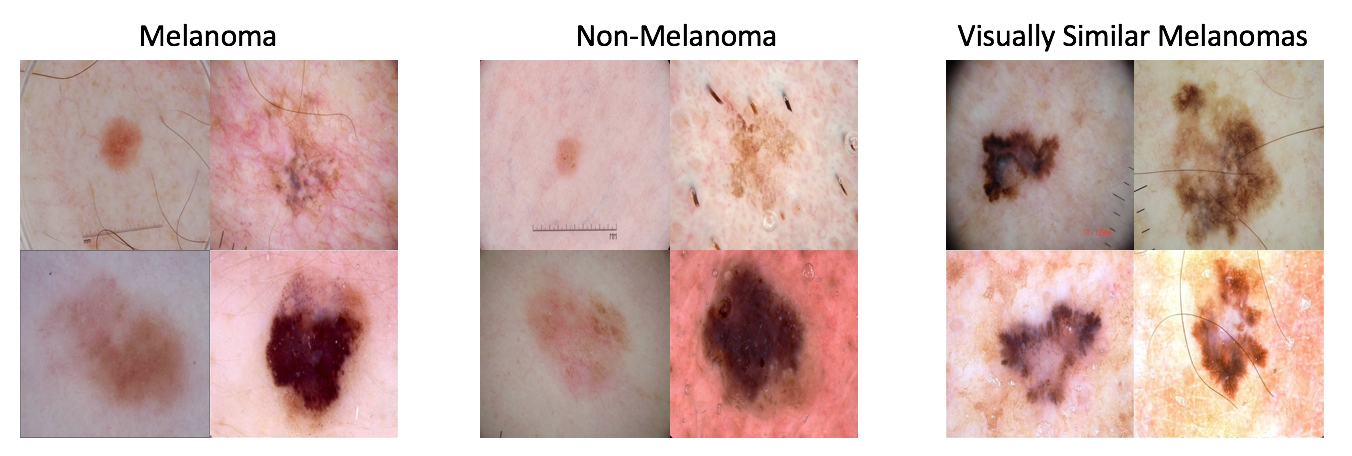
Figure 1: Example images from the ISIC Melanoma detection dataset. The visual similarity between Melanoma and non-Melanoma images is seen from the left and middle images. In the right image, the visually similar lesions are placed in the same group (i.e., have the same $e$ value).

The 2017 International Skin Imaging Collaboration (ISIC) challenge on Skin Lesion Analysis Toward Melanoma Detection dataset (Codella et al., 2018a) is a public dataset with $2000$ training and $600$ test images. Each image belongs to one of the three classes: melanoma (513 images), seborrheic keratosis (339 images) and benign nevus (1748 images). We use a version of this dataset described by Codella et al. (2018b), where the melanoma images were partitioned to 20 groups, the seborrheic keratosis images were divided into 12 groups, and 15 groups were created for benign nevus, by a non-expert human user. We show some example images from this dataset in Figure 1. We take the $3$ class labels to be $Y$ and the $47$ total groups to be $E$. In this dataset, each $e$ maps to a unique $y$. We partition the original training set into a training set with $1600$ images, and a validation set with $400$ images, for use in our experiments. We continue using the original test set with $600$ images.

4.2 Metrics

An open question that we do not attempt to resolve here is the precise form that explanations should take. It is important that they match the mental model of the explanation consumer. For example, one may expect explanations to be categorical (as in loan approval reason codes or our melanoma dataset) or discrete ordinal, as in human ratings. Explanations may also be continuous in crowd sourced environments, where the final rating is an (weighted) average over the human ratings. This is seen in the Olfactory datasets that we consider, where each explanation is averaged over 49 individuals.

In the Olfactory dataset, since we use the existing continuous-valued attributes as explanations, we choose to treat them both as-is and discretized into $3$ bins, $\{-1,0,1\}$, representing negative, neutral, and positive values. The latter mimics human ratings (e.g., not pleasing, neutral, or pleasing). Specifically, we train on the original continuous $Y$ values and report absolute error (MAE) between $Y$ and a continuous-valued prediction $\hat{Y}$. We also similarly discretize $Y$ and $\hat{Y}$ as $-1,0,1$. We then report both absolute error in the discretized values (so that $\lvert 1-0\rvert=1$ and $\lvert 1-(-1)\rvert=2$) as well as $0$-$1$ error ($\hat{Y}=Y$ or $\hat{Y}\neq Y$), where the latter corresponds to conventional classification accuracy. We use bin thresholds of $33.66$ and $49.68$ for Olfactory to partition the $Y$ scores in the training data into thirds.

The explanations $E$ are treated similarly to $Y$ by computing $\ell_{1}$ distances (sum of absolute differences over attributes) before and after discretizing to $\{-1,0,1\}$. We do not, however, compute the $0$-$1$ error for $E$. We use thresholds of $2.72$ and $6.57$ for Olfactory, which roughly partitions the values into thirds based on the training data.

For the melanoma classification dataset, since both $Y$ and $E$ are categorical, we use classification accuracy as the performance metric for both $Y$ and $E$.

Table 1: Accuracy of predicting $Y$ and $E$ for ISIC (left) and Olfactory (right) using different methods (Section 3.2). For ISIC, Baseline for $Y$ and $E$ are classification networks. For Olfactory, Baseline LASSO and RF predict $Y$ from $X$. Multi-task LASSO regression with $\ell_{21}$ regularization on the coefficient matrix predicts Y&E together, or just $E$. For both, Multi-task learning predicts both $Y$ and $E$ together, Embedding $Y$ + $k$NN uses the embedding from the last hidden layer of the baseline network that predicts $Y$. Pairwise $Y$ + $k$NN and Pairwise $E$ + $k$NN use the cosine embedding loss in (1) and (2) respectively to optimize the embeddings of $X$. Pairwise $Y$ & $E$ + $k$NN uses the sum of cosine embedding losses in (3) to optimize the embeddings of $X$.

Algorithm	$\lambda$ or K	Y Accuracy	E Accuracy
Baseline ($Y$)	NA	0.7045	NA
Baseline ($E$)	NA	0.6628	0.4107
	0.01	0.6711	0.2838
	0.1	0.6644	0.2838
	1	0.6544	0.4474
Multi-task	10	0.6778	0.4274
classification	25	0.7145	0.4324
($Y$ & $E$)	50	0.6694	0.4057
	100	0.6761	0.4140
	250	0.6711	0.3957
	500	0.6327	0.3907
	1	0.6962	0.2604
Embedding $Y$	2	0.6995	0.2604
+	5	0.6978	0.2604
$k$NN	10	0.6962	0.2604
	15	0.6978	0.2604
	20	0.6995	0.2604
	1	0.6978	0.4357
Embedding $E$	2	0.6861	0.4357
+	5	0.6861	0.4357
$k$NN	10	0.6745	0.4407
	15	0.6828	0.4374
	20	0.6661	0.4424
	1	0.7162	0.1619
Pairwise $Y$	2	0.7179	0.1619
+	5	0.7179	0.1619
$k$NN	10	0.7162	0.1619
	15	0.7162	0.1619
	20	0.7162	0.1619
	1	0.7245	0.3406
Pairwise $E$	2	0.7279	0.3406
+	5	0.7229	0.3389
$k$NN	10	0.7279	0.3389
	15	0.7329	0.3372
	20	0.7312	0.3356

		Performance on Y			Performance on E
			MAE		MAE
Algorithm	$k$	Class. Accuracy	Discretized	Continuous	Discretized	Continuous
Baseline LASSO ($Y$)	NA	0.4928	0.5072	8.6483	NA	NA
Baseline RF ($Y$)	NA	0.5217	0.4783	8.9447	NA	NA
Multi-task
regression	NA	0.4493	0.5507	11.4651	0.5034	3.6536
($Y$ & $E$)
Multi-task
regression	NA	NA	NA	NA	0.5124	3.3659
($E$ only)
	1	0.5362	0.5362	11.7542	0.5690	4.2050
Embedding $Y$	2	0.5362	0.4928	9.9780	0.4950	3.6555
+	5	0.6087	0.4058	9.2840	0.4516	3.3488
$k$NN	10	0.5652	0.4783	10.1398	0.4622	3.4128
	15	0.5362	0.4928	10.4433	0.4798	3.4012
	20	0.4783	0.5652	10.9867	0.4813	3.4746
	1	0.6087	0.4783	10.9306	0.5515	4.3547
Pairwise $Y$	2	0.5362	0.5072	10.9274	0.5095	3.9330
+	5	0.5507	0.4638	10.4720	0.4935	3.6824
$k$NN	10	0.5072	0.5072	10.7297	0.4912	3.5969
	15	0.5217	0.4928	10.6659	0.4889	3.6277
	20	0.4638	0.5507	10.5957	0.4889	3.6576
	1	0.6087	0.4493	11.4919	0.5728	4.2644
Pairwise $E$	2	0.4928	0.5072	9.7964	0.5072	3.7131
+	5	0.5507	0.4493	9.6680	0.4767	3.4489
$k$NN	10	0.5507	0.4493	9.9089	0.4897	3.4294
	15	0.4928	0.5072	10.1360	0.4844	3.4077
	20	0.4928	0.5072	10.0589	0.4760	3.3877
	1	0.6522	0.3913	10.4714	0.5431	4.0833
Pairwise $Y$&$E$	2	0.5362	0.4783	10.0081	0.4882	3.6610
+	5	0.5652	0.4638	10.0519	0.4622	3.4735
$k$NN	10	0.5072	0.5217	10.3872	0.4653	3.4786
	15	0.5072	0.5217	10.7218	0.4737	3.4955
	20	0.4493	0.5797	10.8590	0.4790	3.5027

4.3 Melanoma

We use all the approaches proposed in Section 3.2 to obtain results for the Melanoma dataset: (a) simple regression baselines for predicting $Y$ and for predicting $E$, (b) multi-task classification to predict $Y$ and $E$ together, (c) $k$NN using embeddings from the simple regression network ($Y$), and from the baseline $E$ network, (d) $k$NN using embeddings optimized for pairwise loss using $Y$, and using $E$. We do not obtain embeddings using weighted pairwise loss with $Y$ and $E$ because there is a one-to-one map from $E$ to $Y$ in this dataset.

The networks used a modified PyTorch implementation of AlexNet for fine-tuning (Krizhevsky et al., 2012). We simplified the fully connected layers for the regression variant of AlexNet to 1024-ReLU-Dropout-64-$n$, where $n=1$ for predicting $Y$, and $n=11$ for predicting $E$. We used cross-entropy losses.

In the multi-task case for predicting $Y$ and $E$ together, the convolutional layers were shared and two separate sets of fully connected layers with $1$ and $11$ outputs were used. The multi-task network used a weighted sum of regression losses for $Y$ and $E$: $\text{loss}_{Y}+\lambda\text{loss}_{E}$. All these single-task and multi-task networks were trained for $100$ epochs with a batch size of 64. The embedding layer that provides the $64-$dimensional output had a learning rate of $0.01$, whereas all other layers had a learning rate of $0.001$. For training the embeddings using pairwise losses, we used $100,000$ pairs chosen from the training data, and optimized the loss for $15$ epochs. The hyper-parameters $(m_{1},m_{2})$ were set to $(0.75,0.75)$, and were chosen to based on the validation set performance. For the loss (1), $a$ and $b$ were said to be neighbors if $y_{a}=y_{b}$ and non-neighbors otherwise. For the loss (2), $a$ and $b$ were said to be neighbors if $z_{a}=z_{b}$ and non-neighbors $y_{a}\neq y_{b}$. The pairs where $z_{a}\neq z_{b}$, but $y_{a}=y_{b}$ were not considered.

The left side of Table 1 provides accuracy numbers for $Y$ and $E$ using the proposed approaches. Numbers in bold are the best for a metric among an algorithm. The $Y$ and $E$ accuracies for multi-task and $k$NN approaches are better than that the baselines, which clearly indicates the value in sharing information between $Y$ and $E$. The best accuracy on $Y$ is obtained using the Pairwise $E$ + $k$NN approach, which is not surprising since $E$ contains $Y$ and is more granular than $Y$. Pairwise $Y$ + $k$NN approach has a poor performance on $E$ since the information in $Y$ is too coarse for predicting $E$ well.

4.4 Olfactory

Since random forest was the winning entry on this dataset (Keller et al., 2017), we used a random forest regression to pre-select $200$ out of $4869$ features for subsequent modeling. From these $200$ features, we created a base regression network using fully connected hidden layer of 64 units (embedding layer), which was then connected to an output layer. No non-linearities were employed, but the data was first transformed using $\log 10(100+x)$ and then the features were standardized to zero mean and unit variance. Batch size was 338, and the network with pairwise loss was run for $750$ epochs with a learning rate of $0.0001$. For this dataset, we set $(c_{1},c_{2},c_{3},c_{4},m_{1},m_{2},w)$ to $(10,20,0.0272,0.0272,0.25,0.25,1.0)$. The parameters were chosen to maximize performance on the validation set.

The right side of Table 1 provides accuracy numbers in a similar format as the left side. The results show, once again, improved $Y$ accuracy over the baseline for Pairwise $Y$ + $k$NN and Pairwise $Y$ & $E$ + $k$NN and corresponding improvement for MAE for $Y$. Again, this performance improvement can be explained by the fact that the predictive accuracy of $Y$ given $E$ using the both baselines were $0.8261$, with MAEs of $0.1739$ and $3.4154$ ($4.0175$ for RF) for Discretized and Continuous, respectively. Once again, the accuracy of $E$ varies among the 3 $k$NN techniques with no clear advantages. The multi-task linear regression does not perform as well as the Pairwise loss based approaches that use non-linear networks.

5 Discussion

Hind et al. (2019) discuss the additional labor required for providing training explanations. Researchers (Zaidan & Eisner, 2008; Zhang et al., 2016; McDonnell et al., 2016) have quantified that for an expert SME, the time to add labels and explanations is often the same as just adding labels and cite other benefits, such as improved quality and consistency of the resulting training data set. Furthermore, in some instances, the $k$NN instantiation of TED may require no extra labor. For example, when embeddings are used as search criteria for evidence-based predictions of queries, end users will, on average, naturally interact with search results that are similar to the query in explanation space. This query-result interaction activity inherently provides similar and dissimilar pairs in the explanation space that can be used to refine an embedding initially optimized for the predictions alone. This reliance on relative distances in explanation space is also what distinguishes this method from multi-task learning objectives, since absolute labels in explanation space need not be defined.

6 Conclusion

The societal demand for “meaningful information” on automated decisions has sparked significant research in AI explanability. This paper describes two novel instantiations of the TED framework. The first learns feature embeddings using labels and explanation similarities in a joint and aligned way to permit neighbor-based explanation prediction. The second uses labels and explanations together in a multi-task setting. We have demonstrated these two instantiations on a publicly-available olfactory pleasantness dataset (Keller et al., 2017) and Melanoma detection dataset (Codella et al., 2018a). We hope this work will inspire other researchers to further enrich this paradigm.

References

- Ainur et al. (2010) Ainur, Y., Choi, Y., and Cardie, C. Automatically generating annotator rationales to improve sentiment classification. In Proceedings of the ACL 2010 Conference Short Papers, pp. 336–341, 2010.
- Bastani et al. (2018) Bastani, O., Kim, C., and Bastani, H. Interpreting blackbox models via model extraction. arXiv preprint arXiv:1705.08504, 2018.
- Biran & Cotton (2017) Biran, O. and Cotton, C. Explanation and justification in machine learning: A survey. In IJCAI-17 Workshop on Explainable AI (XAI), 2017.
- Breiman (2017) Breiman, L. Classification and regression trees. Routledge, 2017.
- Caruana et al. (2015) Caruana, R., Lou, Y., Gehrke, J., Koch, P., Sturm, M., and Elhadad, N. Intelligible models for healthcare: Predicting pneumonia risk and hospital 30-day readmission. In ACM SIGKDD International Conference Knowledge Discovery and Data Mining, pp. 1721–1730, Sydney, Australia, August 2015.
- Codella et al. (2018a) Codella, N. C., Gutman, D., Celebi, M. E., Helba, B., Marchetti, M. A., Dusza, S. W., Kalloo, A., Liopyris, K., Mishra, N., Kittler, H., et al. Skin lesion analysis toward melanoma detection: A challenge at the 2017 international symposium on biomedical imaging (ISBI), hosted by the international skin imaging collaboration (isic). In Biomedical Imaging (ISBI 2018), 2018 IEEE 15th International Symposium on, pp. 168–172, 2018a.
- Codella et al. (2018b) Codella, N. C., Lin, C.-C., Halpern, A., Hind, M., Feris, R., and Smith, J. R. Collaborative human-ai CHAI: Evidence-based interpretable melanoma classification in dermoscopic images. In MICCAI 2018, Workshop on Interpretability of Machine Intelligence in Medical Image Computing (IMIMIC), 2018b. arXiv preprint arXiv:1805.12234.
- Codella et al. (2018c) Codella, N. C. F., Hind, M., Ramamurthy, K. N., Campbell, M., Dhurandhar, A., Varshney, K. R., Wei, D., and Mojsilovic, A. Teaching meaningful explanations, 2018c. arXiv preprint arXiv:1805.11648.
- Cohen (1995) Cohen, W. W. Fast effective rule induction. In Machine Learning Proceedings 1995, pp. 115–123. Elsevier, 1995.
- Dash et al. (2018) Dash, S., Gunluk, O., and Wei, D. Boolean decision rules via column generation. In Advances in Neural Information Processing Systems, pp. 4655–4665, 2018.
- Dhurandhar et al. (2017) Dhurandhar, A., Iyengar, V., Luss, R., and Shanmugam, K. A formal framework to characterize interpretability of procedures. In ICML Workshop on Human Interpretable Machine Learning (WHI), pp. 1–7, Sydney, Australia, August 2017.
- Donahue & Grauman (2011) Donahue, J. and Grauman, K. Annotator rationales for visual recognition. In ICCV, 2011.
- Doshi-Velez & Kim (2017) Doshi-Velez, F. and Kim, B. Towards a rigorous science of interpretable machine learning, 2017. arXiv preprint arXiv:1702.08608v2.
- Doshi-Velez et al. (2017) Doshi-Velez, F., Mason Kortz, R. B., Bavitz, C., Sam Gershman, D. O., Schieber, S., Waldo, J., Weinberger, D., and Wood, A. Accountability of ai under the law: The role of explanation, 2017. arXiv preprint arXiv:1711.01134.
- Goodman & Flaxman (2016) Goodman, B. and Flaxman, S. EU regulations on algorithmic decision-making and a ‘right to explanation’. pp. 26–30, New York, NY, June 2016.
- Hendricks et al. (2016) Hendricks, L. A., Akata, Z., Rohrbach, M., Donahue, J., Schiele, B., and Darrell, T. Generating visual explanations. In European Conference on Computer Vision, 2016.
- Hind et al. (2019) Hind, M., Wei, D., Campbell, M., Codella, N. C. F., Dhurandhar, A., Mojsilovic, A., Ramamurthy, K. N., and Varshney, K. R. TED: Teaching AI to explain its decisions. In AAAI/ACM conference on Artificial Intelligence, Ethics, and Society, 2019.
- Jimenez-del-Toro et al. (2015) Jimenez-del-Toro, O., Hanbury, A., Langs, G., Foncubierta–Rodriguez, A., and Muller, H. Overview of the visceral retrieval benchmark 2015. In Multimodal Retrieval in the Medical Domain (MRMD) Workshop, in the 37th European Conference on Information Retrieval (ECIR), 2015.
- Keller et al. (2017) Keller, A., Gerkin, R. C., Guan, Y., Dhurandhar, A., Turu, G., Szalai, B., Mainland, J. D., Ihara, Y., Yu, C. W., Wolfinger, R., Vens, C., Schietgat, L., De Grave, K., Norel, R., Stolovitzky, G., Cecchi, G. A., Vosshall, L. B., and Meyer, P. Predicting human olfactory perception from chemical features of odor molecules. Science, 355(6327):820–826, 2017.
- Kong et al. (2016) Kong, S., Shen, X., Lin, Z., Mech, R., and Fowlkes, C. Photo aesthetics ranking network with attributes and content adaptation. In European Conference on Computer Vision, pp. 662–679, Amsterdam, Netherlands, October 2016.
- Krizhevsky et al. (2012) Krizhevsky, A., Sutskever, I., and Hinton, G. E. Imagenet classification with deep convolutional neural networks. In Advances in Neural Information Processing Systems, 25, pp. 1097–1105. 2012.
- Lei et al. (2016) Lei, T., Barzilay, R., and Jaakkola, T. Rationalizing neural predictions. In EMNLP, 2016.
- Li et al. (2018) Li, Z., Zhang, X., Muller, H., and Zhang, S. Large-scale retrieval for medical image analytics: A comprehensive review. In Medical Image Analysis, volume 43, pp. 66–84, 2018.
- Lundberg & Lee (2017) Lundberg, S. and Lee, S.-I. A unified approach to interpreting model predictions. In Advances of Neural Information Processing Systems, 2017.
- McDonnell et al. (2016) McDonnell, T., Lease, M., Kutlu, M., and Elsayed, T. Why is that relevant? collecting annotator rationales for relevance judgments. In AAAI Conference on Human Compututing Crowdsourcing, 2016.
- Miller (2017) Miller, T. Explanation in artificial intelligence: Insights from the social sciences. arXiv preprint arXiv:1706.07269, June 2017.
- Miller et al. (2017) Miller, T., Howe, P., and Sonenberg, L. Explainable AI: Beware of inmates running the asylum or: How I learnt to stop worrying and love the social and behavioural sciences. In Proc. IJCAI Workshop Explainable Artif. Intell., Melbourne, Australia, August 2017.
- Montavon et al. (2017) Montavon, G., Samek, W., and Müller, K.-R. Methods for interpreting and understanding deep neural networks. Digital Signal Processing, 2017.
- Peng et al. (2016) Peng, P., Tian, Y., Xiang, T., Wang, Y., and Huang, T. Joint learning of semantic and latent attributes. In ECCV 2016, Lecture Notes in Computer Science, volume 9908, 2016.
- Ribeiro et al. (2016) Ribeiro, M. T., Singh, S., and Guestrin, C. “Why should I trust you?”: Explaining the predictions of any classifier. In Proc. ACM SIGKDD Int. Conf. Knowl. Disc. Data Min., pp. 1135–1144, San Francisco, CA, August 2016.
- Selbst & Powles (2017) Selbst, A. D. and Powles, J. Meaningful information and the right to explanation. International Data Privacy Law, 7(4):233–242, November 2017.
- Sun et al. (2012) Sun, J., Wang, F., Hu, J., and Edabollahi, S. Supervised patient similarity measure of heterogeneous patient records. In SIGKDD Explorations, 2012.
- Sun & DeJong (2005) Sun, Q. and DeJong, G. Explanation-augmented svm: an approach to incorporating domain knowledge into svm learning. In 22nd International Conference on Machine Learning, 2005.
- Wachter et al. (2017) Wachter, S., Mittelstadt, B., and Floridi, L. Why a right to explanation of automated decision-making does not exist in the general data protection regulation. International Data Privacy Law, 7(2):76–99, May 2017.
- Wan et al. (2014) Wan, J., Wang, D., Hoi, S., Wu, P., Zhu, J., Zhang, Y., and Li, J. Deep learning for content-based image retrieval: A comprehensive study. In Proceedings of the ACM International Conference on Multimedia, 2014.
- Wang et al. (2017) Wang, T., Rudin, C., Doshi-Velez, F., Liu, Y., Klampfl, E., and MacNeille, P. A bayesian framework for learning rule sets for interpretable classification. Journal of Machine Learning Research, 18(70):1–37, 2017.
- Zaidan & Eisner (2008) Zaidan, O. F. and Eisner, J. Modeling annotators: A generative approach to learning from annotator rationales. In Proceedings of EMNLP 2008, pp. 31–40, October 2008.
- Zhang et al. (2016) Zhang, Y., Marshall, I. J., and Wallace, B. C. Rationale-augmented convolutional neural networks for text classification. In Conference on Empirical Methods in Natural Language Processing (EMNLP), 2016.