Experimental simultaneous read out of the real and imaginary parts of the weak value

Abstract

The weak value, the average result of a weak measurement, has proven useful for probing quantum and classical systems. Examples include the amplification of small signals, investigating quantum paradoxes, and elucidating fundamental quantum phenomena such as geometric phase. A key characteristic of the weak value is that it can be complex, in contrast to a standard expectation value. However, typically only either the real or imaginary component of the weak value is determined in a given experimental setup. Weak measurements can be used to, in a sense, simultaneously measure non-commuting observables. This principle was used in the direct measurement of the quantum wavefunction. However, the wavefunction’s real and imaginary components, given by a weak value, are determined in different setups or on separate ensembles of systems, putting the procedure’s directness in question. To address these issues, we introduce and experimentally demonstrate a general method to simultaneously read out both components of the weak value in a single experimental apparatus. In particular, we directly measure the polarization state of an ensemble of photons using weak measurement. With our method, each photon contributes to both the real and imaginary parts of the weak-value average. On a fundamental level, this suggests that the full complex weak value is a characteristic of each photon measured.

I Introduction

Weak values and weak measurement have attracted a considerable amount of interest in recent years Dressel et al. (2014). Weak values were introduced in 1988 Aharonov et al. (1988a); Aharonov and Vaidman (1989) as the average result of a gently probing measurement (i.e., a ‘weak measurement’) of an quantum observable for an input quantum state and followed by a projective measurement. They have been used to investigate quantum paradoxes, such as the three-box Aharonov and Vaidman (1991); Resch et al. (2004), the Cheshire Cat Aharonov et al. (2013); Denkmayr et al. (2014), and Hardy’s paradoxes Aharonov et al. (2002); Lundeen and Steinberg (2009). Weak values are deeply connected to other fundamental and uniquely quantum phenomena, such as geometric phase Sjöqvist (2006), time-reversal symmetry violation Aharonov et al. (1964); Bednorz et al. (2013); Curic et al. (2018), Bayesian quantum estimation Johansen (2004), and non-contextuality Tollaksen (2007); Dressel et al. (2010); Pusey (2014). They have also found application in the field of metrology. In a technique called ‘weak-value amplification’, the weak value can become much larger than the standard expectation value of an observable, thereby amplifying the associated measurement signal Aharonov et al. (1988a). This has been used to measure small shifts in quantities such as phase, time, frequency, angle, and temperature Hosten and Kwiat (2008); Starling et al. (2009, 2010); Brunner and Simon (2010); Egan and Stone (2012).

Most relevant to this work, weak measurement has been used to directly measure the quantum wavefunction of a system Lundeen et al. (2011a); Lundeen and Bamber (2012); Bamber and Lundeen (2014); Thekkadath et al. (2016). This procedure weakly measures one variable (e.g., position $x$) and then strongly measures the complementary variable (e.g., momentum $p$). The real and imaginary parts of the wavefunction $\psi(x)$ appear directly on the measurement apparatus as the real and imaginary parts of the weak value. In this way, an unknown input quantum state can be determined. And, in contrast to quantum state tomography, this can be accomplished without the need for a complicated mathematical reconstruction such as an inversion or fitting. Nevertheless, there has been a degree of indirectness in almost all experiments that measure both the real and imaginary parts of the weak value. In particular, each part is measured by averaging over a separate sub-ensemble. This happens in two possible ways: 1. A different apparatus is used to measure each of the two parts. 2. A single apparatus randomly chooses whether it is the real or imaginary part that is measured in a given trial. In either case, the real and imaginary parts of the wavefunction are determined separately, which diminishes the purported directness of the technique.

Another motivation for this work is to establish whether the weak value is fundamental to a physical system. The experiments described above suggest that measurements of the real and the imaginary parts of the weak value are mutually exclusive. It may be fundamentally impossible to measure them simultaneously, much like the Heisenberg Uncertainty Principle forbids the simultaneous precise measurement of complementary observables. If true, it may be incorrect to consider both the real and imaginary parts of the weak value as the average result of weak measurement or as simultaneous properties of the measured system. This would contradict particular interpretations of quantum physics that take weak values as deterministic (i.e., ‘real’ or ontological) properties of a system Aharonov and Vaidman (1991); Vaidman (1996); Hofmann (2012).

Recently, an experiment demonstrated the simultaneous read out of the real and imaginary parts of the weak value using orbital angular momentum states of light Kobayashi et al. (2014). However, it was unclear whether orbital angular momentum was inherently necessary or whether the technique was more general. In this work, we show that the technique in Ref. Kobayashi et al. (2014) can be generalized to a broad class of weak measurement implementations by performing a sequence of two separate weak measurements of the same observable. We experimentally demonstrate the method by directly measuring the polarization state of an ensemble of photons while simultaneously reading out both the real and imaginary parts of the weak value for each photon.

We begin by reviewing the theory behind weak values. We then theoretically introduce the two above mentioned general methods to concurrently measure the real and imaginary parts of the weak value. Next, we describe an experiment in which we directly measure the photon polarization state.

II Theoretical Description of Weak Measurement

The concept of weak measurement is best introduced within von Neumann’s model of quantum measurement. Arguably, any type of measurement can be described with it Wiseman and Milburn (2010). The key feature of this model that distinguishes it from the standard treatment of measurement in quantum mechanics is that both the measured system $S$ and the ‘pointer’ $P$ of measurement apparatus are treated quantum mechanically. That is, both have quantum states. The measured system begins in an arbitrary superposition state $|\psi\rangle_{S}=\sum_{n}c_{n}|a_{n}\rangle_{S}$, where $|a_{n}\rangle_{S}$ is an eigenstate of the observable $\hat{A}$ that is to be measured, with eigenvalue $a_{n}$. The measurement apparatus incorporates a pointer that will indicate the result of the measurement. The pointer is in state $|\xi\rangle_{P}$. Initially, $|\xi\rangle_{P}=|\bar{q}=0\rangle_{P}$, a state with standard deviation $\sigma$ and center $\bar{q}$ in some variable $q$ (e.g., position). Together, the pointer and measured system compose the total system $T$, which has state $|\Theta\rangle_{T}=|\psi\rangle_{S}\otimes|\bar{q}=0\rangle_{P}$ initially.

To perform the measurement, the system observable is coupled to the conjugate pointer variable $k$ (e.g., momentum) by the von Neumann measurement interaction

$$\hat{U}=\mathrm{exp}(-i\delta\hat{A}\otimes\hat{k}),$$ (1)

where $\delta$ is the coupling strength. The action of unitary $\hat{U}$ is as follows. The pointer will be shifted by $\Delta q=\delta a_{n}$ for state $|a_{n}\rangle_{S}$ in $|\psi\rangle_{S}$. Thus, the final state of the total system is given by $|\Theta^{\prime}\rangle_{T}=\sum_{n}c_{n}|a_{n}\rangle_{S}|q=\delta a_{n}\rangle_{P}$, which is now entangled between $S$ and $P$. Lastly, in the ‘read out’ step of the model, one measures $\hat{q}$ on the pointer to read out the measurement of $\hat{A}$. If the shift is large compared to the initial spread of the pointer, $\delta\gg\sigma$, then the outcome of the measurement can be read out unambiguously in a single trial with minimal error. However, given outcome $a_{n}$, the system will then be left in a single state $|a_{n}\rangle_{S}$, destroying the initial superposition (i.e., ‘collapse’). This is a standard (i.e. ‘strong’) measurement.

The opposite limit, $\delta\ll\sigma$, defines the regime of weak measurement. In this limit, the shifted pointer states in $|\Theta^{\prime}\rangle_{T}$ overlap in $q$, making the result of the measurement ambiguous in any given trial. However, since the the measured system is now only minimally entangled with the pointer, reading out $\hat{A}$ by measuring $\hat{q}$ now only minimally disturbs the initial measured-system state $|\psi\rangle_{S}$. Subsequent measurement will now reveal additional information about that state. Consider a subsequent projective measurement onto state $|\varphi\rangle_{S}$. In the sub-ensemble of trials that have been successfully projected onto $|\varphi\rangle_{S}$ (i.e., ‘post-selection’), the pointer will on average be shifted by an amount proportional to the ‘weak value’ Aharonov et al. (1988b):

$$\langle\hat{A}\rangle_{W}=\frac{\langle\varphi|\hat{A|}\psi\rangle}{\langle\varphi|\psi\rangle}.$$ (2)

For this to be valid, the pointer shift, $\delta\langle\hat{A}\rangle_{W}$ (i.e., the ‘signal’), must be much smaller than the pointer spread $\sigma$ (i.e., the ‘noise’) Duck et al. (1989). In other words, for a single trial the signal to noise ratio in a weak measurement is small. Nonetheless, by repeating the weak measurement in a large number of trials one can reduce the effect of noise by averaging. The average result is the weak value.

Unlike standard expectation values, the weak value can be complex valued. The real and imaginary parts of the weak value manifest as shifts in the two conjugate pointer variables $q$ and $k$:

$$\langle\hat{A}\rangle_{W}=\frac{1}{\delta}\left(\left\langle\hat{q}\right\rangle+i4\sigma^{2}\left\langle\hat{k}\right\rangle\right),$$ (3)

where the expectation values on the right-hand side are taken for the final pointer state.

The heart of the problem of determining $\mathrm{Re}\langle\hat{A}\rangle_{W}$ and $\mathrm{Im}\langle\hat{A}\rangle_{W}$ simultaneously is that $\hat{q}$ and $\hat{k}$ do not commute, and, thus, can not be measured at the same time. Instead, past experiments have measured $\mathrm{Re}\langle\hat{A}\rangle_{W}$ and $\mathrm{Im}\langle\hat{A}\rangle_{W}$ on separate sub-ensembles of the measured system. This was achieved with one of two methods, which we call Method A and Method B (see Fig. 1). In Method A, the ensemble is divided in two. Each sub-ensemble is then sent through the von Neumann interaction (i.e., Eq. 1) and to the subsequent strong projective measurement. In the final step, the reading out of the weak measurement, only one of the pointer variables, $q$ or $k$, is measured for each sub-ensemble. An example of this strategy is the original direct measurement of the wavefunction experiment Lundeen et al. (2011b). There, the photon’s polarization was used as a pointer. The two conjugate pointer observables were $\hat{\sigma}_{x}$ and $\hat{\sigma}_{y}$, the polarization Pauli matrices. One Pauli matrix or the other was chosen to be measured by setting the angle of a waveplate. Thus, $\mathrm{Re}\langle\hat{A}\rangle_{W}$ and $\mathrm{Im}\langle\hat{A}\rangle_{W}$ were determined separately for two sub-ensembles of photons delineated by time.

In Method B, the ensemble is divided after the von Neumann interaction and subsequent strong measurement. An example of this is in another direct measurement experiment Salvail et al. (2013). In it, the photon’s polarization was the measured system and its transverse spatial mode was used as the pointer. Just before the weak-measurement read out, a beamsplitter divided the ensemble of photons in two. For one sub-ensemble the transverse momentum was measured. For the other sub-ensemble the transverse photon position was measured. In this way, in each trial either the pointer momentum or position were determined depending on which way the photon exited the beamsplitter. Consequently, the real and imaginary weak values were determined with distinct sub-ensembles.

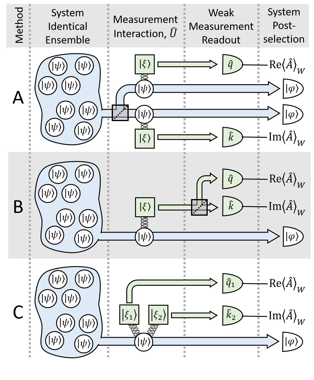
Figure 1: Schemes for measuring the real and imaginary parts of the weak value, $\mathrm{Re}\langle\hat{A}\rangle_{W}$ and $\mathrm{Im}\langle\hat{A}\rangle_{W}$. In Method A, an identical ensemble of system states $|\psi\rangle_{S}$ is divided into two before the von Neumann measurement interaction $\hat{U}$ couples system observable $\hat{A}$ to the pointer $P$, initially in state $|\xi\rangle_{P}$. One sub-ensemble is then used to read out $\mathrm{Re}\langle\hat{A}\rangle_{W}$ from the pointer. The other sub-ensemble is used to read out $\mathrm{Im}\langle\hat{A}\rangle_{W}$. Method B is similar except that the division into two sub-ensembles happens after the measurement interaction. In Method C, two pointers are coupled to the system in two measurement interactions. One pointer is used to read out $\mathrm{Re}\langle\hat{A}\rangle_{W}$ while the other is used read out $\mathrm{Im}\langle\hat{A}\rangle_{W}$. Only in Method C does each member of the identical ensemble contribute to the read out of the full complex weak.

III A General Method to Measure the Full Complex Weak Value

We now introduce Method C (Fig. 1), which allows one to determine the real and imaginary parts of the weak value simultaneously. This was first achieved in Ref. Kobayashi et al. (2014) by using an orbital angular momentum pointer, which had a ring-like transverse probability distribution. Shifts of the center of the ring along two orthogonal directions gave the two parts of the weak value. While in Ref. Kobayashi et al. (2014) this is framed as an effect that relies on orbital angular momentum, we will show that the key to the simultaneous determination is the use of the two spatial directions as independent pointers.

Since weak measurements minimize disturbance to the system, multiple weak measurements can be performed in sequence without altering their individual results, i.e. weak values. Consider, two weak measurements but of the same system observable $\hat{A}$. A pointer $P1$ is used for the first von Neumann interaction and, then, another pointer $P2$, is used for the second von Neumann interaction (Eq. 1) giving a total evolution of

$$\hat{U} = \mathrm{exp}\left(-i\delta_{1}\hat{A}\hat{k}_{1}\right)\mathrm{exp}\left(-i\delta_{2}\hat{A}\hat{k}_{2}\right)$$ (4)

$$= \mathrm{exp}\left(-i\hat{A}\left(\delta_{1}\hat{k}_{1}+\delta_{2}\hat{k}_{2}\right)\right),$$ (5)

where $\hat{k}_{j}$ is observable $\hat{k}$ for the $j$-th pointer (and likewise for $\hat{q}$). While $\hat{q}$ and $\hat{k}$ for an individual pointer do not commute, $\hat{q}_{1}$ and $\hat{k}_{2}$ do commute. Consequently, the weak value can now be determined by measuring $\hat{q}_{1}$ for the first pointer and simultaneously measuring $\hat{k}_{2}$ for the second pointer:

$$\langle\hat{A}\rangle_{W}=\frac{1}{\delta_{1}}\left\langle\hat{q}_{1}\right\rangle+i\frac{4\sigma_{2}^{2}}{\delta_{2}}\left\langle\hat{k}_{2}\right\rangle.$$ (6)

Note that the two pointers need not be the same type of quantum systems. They could be an electron and photon, for example. As well, the pointer degrees of freedom, $q_{1}$ and $q_{2}$, might be distinctly different, e.g. spin and position. This procedure, based on a sequence of two weak measurements of $\hat{A}$, constitutes our method to simultaneously measure both parts of the weak value. A given trial will contribute to the average for both $\mathrm{Re}\langle\hat{A}\rangle_{W}$ and $\mathrm{Im}\langle\hat{A}\rangle_{W}$.

IV Experiment to Simultaneously Measure The Full Weak Value

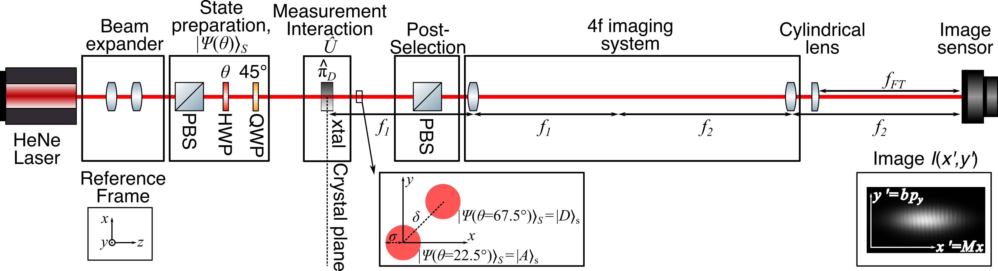
Figure 2: Experimental setup for simultaneous read out of the real and imaginary parts of the weak value. This setup implements Method C in Fig. 1. To create the input polarization state $|\psi(\theta)\rangle_{S}$ (the state of the measured system) we use a polarizing beamsplitter (PBS), half-waveplate (HWP) at angle $\theta$, and quarter-waveplate (QWP). The pointers are the two transverse degrees of freedom of the photon, $x$ and $y$. A beam expander sets the width $\sigma$ of the pointer states. The walk-off crystal (xtal) displaces the two-dimensional pointer along the diagonal direction by $\delta$ if the system is diagonally polarized, $|D\rangle_{S}$. This implements the measurement interaction by coupling the pointer to the observable $\hat{\pi}_{D}$. A 4f lens arrangement images the crystal plane onto an image sensor. The cylindrical lens is used to Fourier transform the spatial distribution solely along the $y$ axis. The image sensor records the average photon number at a pixel index $(n_{x^{\prime}},n_{y^{\prime}})$. This index is proportional to $(x,p_{y})$. By evaluating the pointer shifts, $\langle\hat{x}\rangle$ and $\langle\hat{p_{y}}\rangle$, we find $\mathrm{Re}\langle\hat{\pi}_{D}\rangle_{W}$ and $\mathrm{Im}\langle\hat{\pi}_{D}\rangle_{W}$ via Eq. 6.

We demonstrate Method C by directly measuring the polarization state of a photon. We describe the direct measurement concept in the Appendix. Since photons typically do not interact strongly with other quantum systems, instead of using an external system as a pointer, we use two photonic degrees of freedom as the system and pointer, polarization and transverse mode. This allows us to use linear optics to implement the von Neumann interaction, which will couple a polarization observable to the transverse position of the photon.

For a two-dimensional pointer, such as transverse position, Method C can be significantly simplified. A photon traveling along $z$ has transverse position $(x,y),$ so that $q_{1}=x$ and $q_{2}=y$. Consider if the two couplings are equal, $\delta_{1}=\delta_{2}\equiv\sqrt{2}\delta$. With this, the two-pointer unitary in Eq. 4 reverts to the standard von Neumann interaction (Eq. 1) with a single pointer and a single pointer degree of freedom:

$$\hat{U}=\mathrm{exp}\left(-i\delta\hat{A}\hat{p}_{D}/\hbar\right),$$ (7)

where $\hat{x}_{D}=(\hat{x}+\hat{y})/\sqrt{2}$ is the photon position along the diagonal direction $D$ (it is the $\sqrt{2}$ in $\hat{x}_{D}$ that necessitates the $\sqrt{2}$ in $\delta$). While, we now only require the standard von-Neumann single-pointer unitary interaction (Eq. 1), the final pointer readout must still be two-dimensional. That is both $x$ and the transverse momentum $p_{y}$ (i.e., along $y$) must be measured in order to simultaneously evaluate both $\mathrm{Re}\langle\hat{A}\rangle_{W}$ and $\mathrm{Im}\langle\hat{A}\rangle_{W}$ according to Eq. 6.

The experimental setup is shown in Fig. 2. Our ensemble of photons is produced by a Helium-Neon laser with a wavelength of $\lambda=633$ nm. A polarizing beamsplitter (PBS) sets the photon polarization state to horizontal $|H\rangle_{S}$. The spatial distribution is Gaussian in both the $x$ and $y$ directions and is set to have a $1/e^{2}$ half-width of $\sigma=\sigma_{x}=\sigma_{y}=306\pm 2$ $\upmu\mathrm{m}$ with a beam expander. We use a half-waveplate (HWP) with its optical axis at an angle $\theta$ from the horizontal followed by a quarter-waveplate (QWP) with its axis $-45^{\circ}$ from the horizontal to produce an input polarization state,

$$|\psi(\theta)\rangle_{S} = c_{D}|D\rangle_{S}+c_{A}|A\rangle_{S}$$

$$= \sin(2\theta-\pi/4)|D\rangle_{S}-i\cos(2\theta-\pi/4)|A\rangle_{S},$$

where $|D\rangle$ and $|A\rangle$ are the diagonal and anti-diagonal polarization states, respectively. In order to test our method with a range of system states, we vary $|\psi(\theta)\rangle_{S}$ by rotating the angle $\theta$ of the HWP.

We implement the von Neumann interaction by using a birefringent crystal (Beta Barium Borate) to couple the polarization of the photon to its spatial distribution. A photon with a polarization along the crystal optical axis will be transversely displaced along the direction of the axis, whereas a photon with the orthogonal polarization will not. We use a single crystal (xtal) to displace the position $x_{D}$ of photons with polarization $\left|D\right\rangle_{S}$ by $\delta=163\pm 2$ $\upmu$m. Since $\delta<\sigma$, this interaction is in the weak measurement regime. The weakly measured observable is $\hat{\pi}_{D}\equiv\left|D\right\rangle\left\langle D\right|_{S}$. While, in our case, the displacement and polarization are collinear, by sandwiching such a ‘walk-off crystal’ between waveplates, any polarization projector can be measured.

Following the walk-off crystal, we project the measured system $|\psi\rangle_{S}$ onto the horizontal polarization state $|H\rangle_{S}$ with a polarizing beamsplitter. The transmitted photons are then sent through a 4f lens system (spherical lenses, focal lengths $f_{1}=1$ m and $f_{2}=1.2$ m) that images the crystal plane onto an image sensor (a CMOS sensor with resolution $2560\times 1920$ and a pixel pitch of 2.2 $\upmu\mathrm{m}$ $\times$ 2.2 $\upmu\mathrm{m}$). The final photon position $x^{\prime}$ on the sensor is given by $x^{\prime}=Mx$, where magnification $M=f_{2}/f_{1}=1.2$. The use of a 4f system creates room between the image sensor and the xtal for a long focal length cylindrical lens ($f_{FT}=1$ m, curved along the $y$-direction) to be placed one focal length before the sensor. The cylindrical lens performs a Fourier transform such that the final position is proportional to the initial transverse momentum, $y^{\prime}=bp_{y}$, where $b=\lambda f_{FT}/2\pi\hbar$. The large value of $f_{FT}$ ensures the distribution will cover many pixels in the $y^{\prime}$ direction.

To read out the result of the weak measurement we must determine the average shift of the pointer along $x^{\prime}$ and $y^{\prime}$. Thus, we record the average number of photons (i.e., the intensity) detected at a given position, $I(x^{\prime},y^{\prime})$. From this $\mathrm{Re}\langle\hat{\pi}_{D}\rangle_{W}$ and $\mathrm{Im}\langle\hat{\pi}_{D}\rangle_{W}$ can be calculated by taking $x=x^{\prime}/M$ and $p_{y}=y^{\prime}/b$ in Eq. 6. However, we do not do this. Because it is more direct, a more accurate method is to calculate the expectation values in terms of pixel index $(n_{x^{\prime}},n_{y^{\prime}})$ rather than position:

$$\langle\hat{A}\rangle_{W}=\frac{1}{\delta_{x^{\prime}}}\left(\left\langle\hat{n}_{x^{\prime}}\right\rangle+i\frac{\sigma_{x^{\prime}}}{\sigma_{y^{\prime}}}\left\langle\hat{n}_{y^{\prime}}\right\rangle\right).$$ (9)

To arrive at this expression, $M$ has been expressed in terms of $\delta_{x^{\prime}}=62.8\pm 0.9$ and $\sigma_{x^{\prime}}=167\pm 1$, which are $\delta$ and $\sigma$ in units of pixels. In addition, $b$ has been expressed in terms of $\sigma_{y^{\prime}}=62.9\pm 0.4$ in units of pixels, the pointer width along the $y^{\prime}$ pixel direction. See Ref. Thekkadath et al. (2016) for the details of this method. We vary input system state $|\psi(\theta)\rangle_{S}$ over range $\theta=0$ to $90^{\circ}$ in $3^{\circ}$ steps. For each step three images were collected and averaged and then used to determine pointer shifts $\left\langle\hat{n}_{x^{\prime}}\right\rangle$ and $\left\langle\hat{n}_{y^{\prime}}\right\rangle$. The full range was stepped through seven times. These seven trials were used to determine the mean pointer shifts and their standard error. Based on these, in the next section, we present the measured weak values.

V Results

In Fig. 3. a) and b), we respectively plot the $\mathrm{Re}\langle\hat{\pi}_{D}\rangle_{W}$ and $\mathrm{Im}\langle\hat{\pi}_{D}\rangle_{W}$ points experimentally determined using Method C. The solid line plotted in each panel of Fig. 3 is the corresponding theoretical prediction:

$$\langle\hat{\pi}_{D}\rangle_{W} = \frac{c_{D}}{c_{D}+c_{A}}$$

$$= \frac{1}{2}\left(1+\cos\left(4\theta+\frac{\pi}{2}\right)\right)-\frac{i}{2}\sin\left(4\theta+\frac{\pi}{2}\right),$$

which is found from Eq. IV and Eq. 6. This weak measurement directly measures the amplitudes of $|\psi\rangle_{S}$. Note that the $c_{A}$ amplitude can be eliminated or determined through normalization $|c_{A}|^{2}=1-|c_{D}|^{2}.$ The phases of the amplitudes are determined up to a global phase that changes with the input state $|\psi\rangle_{S}$.

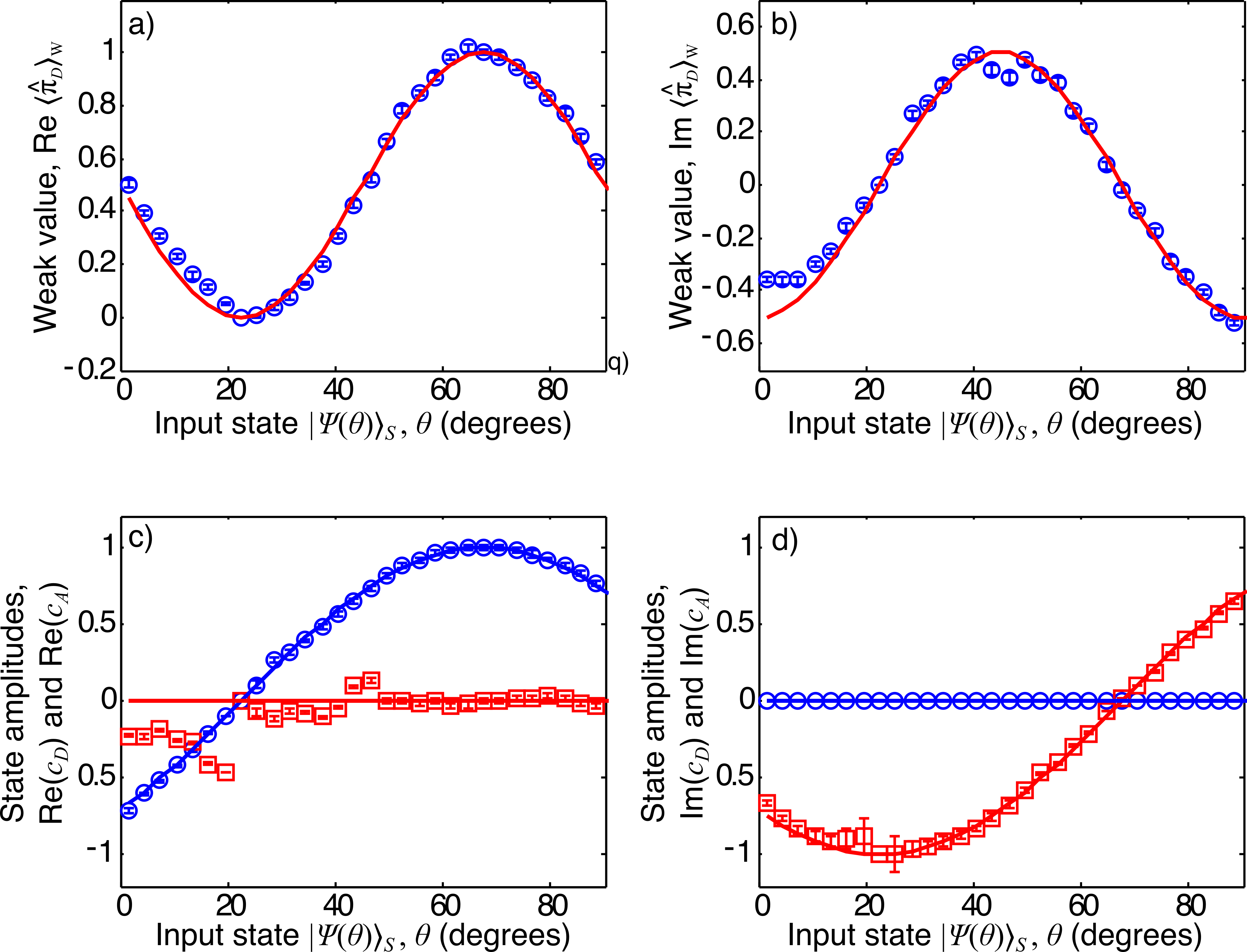
Figure 3: Real and imaginary parts of the measured weak value. In a) and b), we plot the results of a weak measurement of $\hat{\pi}_{D}$ using Method C in Fig. 1. The weak value $\langle\hat{\pi}_{D}\rangle_{W}$ is found from the measured shifts along $x^{\prime}$ and $y^{\prime}$ according to Eq. 9 (blue circles). For system state $|\psi(\theta)\rangle_{S}=c_{D}|D\rangle_{S}+c_{A}|A\rangle_{S}$ the predicted weak value is given by the Eq. V (red line). In c) and d), we use the fact that $\langle\hat{\pi}_{D}\rangle_{W}\varpropto c_{D}$ to directly measure the system state (see the Appendix for details). We plot measured system state amplitudes, $c_{D}$ (blue circles) and $c_{A}$ (red squares). The nominal amplitudes are indicated by the solid lines given by Eq. IV. The error bars indicate the standard error found from repeated trials.

The data points closely follow the theoretical curve, indicating that Method C works. However, they do not agree with theory to within error. We attribute this to systematic errors such as offsets from the nominal birefringent retardance of the waveplates, the axis direction of the crystals, and movement of the beam with waveplate rotation.

VI Discussion and Conclusion

Since the introduction of weak values $\langle\hat{A}\rangle_{W}$ there has been confusion and disagreement about what they represent Leggett (1989); Peres (1989); Aharonov and Vaidman (1989); Ferrie and Combes (2014); Holger F. Hofmann (2014); Brodutch (2015); Ferrie and Combes (2015); Vaidman (2017). Should they be interpreted as the value of the weakly measured parameter Vaidman et al. (2017) (even though it can lie outside the range of the observable’s eigenvalues Aharonov et al. (1988a)), as the average value of that parameter Mir et al. (2007); Kocsis et al. (2011), as a real deterministic property of the measured system Aharonov and Vaidman (1991); Vaidman (1996); Hofmann (2012), or perhaps not regarded as a measurement result at all? This confusion has been compounded by the fact that the weak value is generally complex, in contrast to the standard quantum expectation value. Indeed, in some papers the imaginary part of the weak value is not considered part of the result of the weak measurement at all Wiseman (2003).

There are arguments for and against considering $\mathrm{Im}\langle\hat{A}\rangle_{W}$ as part of the result of the weak measurement. An argument in favour of this is that both $\mathrm{Re}\langle\hat{A}\rangle_{W}$ and $\mathrm{Im}\langle\hat{A}\rangle_{W}$ have clear physical manifestations: as shifts in two conjugate variables of the measurement apparatus pointer, e.g., position and momentum, respectively. An “against” argument is that the appearance of an imaginary component of the average result of a measurement is completely unexpected and, in the context of probability theory, nonsensical. Another “against” argument is that the momentum shift is usually much smaller than the position shift and thus, should be considered a side-effect of the measurement (i.e., reverse ‘back-action’ Steinberg (1995)).

This confusion about the complex nature of the weak value is compounded by the fact that $\mathrm{Re}\langle\hat{A}\rangle_{W}$ and $\mathrm{Im}\langle\hat{A}\rangle_{W}$ were not measured simultaneously in experiments. That is, since the two pointer variables are conjugate, the two shifts could not be determined at the same time. This is particularly consequential when considering the weak-measurement-based concept of direct measurement of the wavefunction. There, the directness is partly a reflection of the full weak value appearing on the measurement apparatus in a straight-forward manner. If the real and imaginary parts do not appear simultaneously then it puts this directness in question.

In this paper, we introduced and experimentally demonstrated a general method to simultaneously measure both the real and imaginary components of the weak value. The method uses a separate pointer and von Neumann measurement interaction for each weak value component. We simplified the method in the case of an inherently two-dimensional system, such as transverse position, so that only one measurement interaction is required. In the method, each and every trial contributes to both the $\mathrm{Re}\langle\hat{A}\rangle_{W}$ and $\mathrm{Im}\langle\hat{A}\rangle_{W}$ averages. Thus, two pointer shifts can manifest themselves at the same time, giving the real and imaginary parts of the wavefunction in a direct measurement. In summary, this paper has provided support to the notion that the full complex weak value should be considered the average result of a weak measurement, and, in that sense, a fundamental property of the measured system.

Appendix: Direct Measurement Of The Quantum State

Our experimental demonstration performs a direct measurement of quantum state. Below we describe what is meant by a direct measurement. Consider if one want to measure the amplitudes of an arbitrary polarization state of a photon expressed in the $A/D$ basis,

$$|\psi\rangle_{S}=c_{D}|D\rangle_{S}+c_{A}|A\rangle_{S},$$ (11)

where $c_{D}=\left\langle D|\psi\right\rangle$ and $c_{A}=\left\langle A|\psi\right\rangle$. We define $|H\rangle,|V\rangle,|D\rangle,$ and $|A\rangle,$ as the horizontal, vertical, diagonal, and anti-diagonal polarization states, where $\left|D\right\rangle=(\left|H\right\rangle+\left|V\right\rangle)/\sqrt{2}$. The concept for direct measurement was introduced in Ref. Lundeen et al. (2011a). In it, a weak measurement of a variable is followed by a strong measurement of a complementary variable. The weak value is proportional to the quantum state. For polarization, this entails weakly measuring $\hat{\pi}_{J}\equiv\left|J\right\rangle\left\langle J\right|$ for $J=A,D$ and then strongly projecting the measured system on $|H\rangle$. A successful projection defines a sub-ensemble of trials in which the average result of the weak measurement, the weak value, is

$$\langle\hat{\pi}_{J}\rangle_{W}=\frac{\langle H|\hat{\pi}_{J}|\psi\rangle}{\langle H|\psi\rangle}=\sqrt{N}\left\langle J|\psi\right\rangle,$$ (12)

where $\sqrt{N}$ is a constant, independent of $J$.

In terms of this weak value, the quantum state is given by,

$$|\psi\rangle_{S} = \frac{1}{\sqrt{N}}\left(\langle\hat{\pi}_{D}\rangle_{W}|D\rangle_{S}+\langle\hat{\pi}_{A}\rangle_{W}|A\rangle_{S}\right)$$ (13)

$$= \frac{1}{\sqrt{N}}\left(\langle\hat{\pi}_{D}\rangle_{W}|D\rangle_{S}+\left(1-\langle\hat{\pi}_{D}\rangle_{W}\right)|A\rangle_{S}\right).$$ (14)

The second line is a simplification using $\hat{I}=\hat{\pi}_{D}+\hat{\pi}_{A}$. Normalization fixes $N=(|\langle\hat{\pi}_{D}\rangle_{W}|^{2}+|1-\langle\hat{\pi}_{D}\rangle_{W}|^{2})$. Typically, one would also fix the global phase, which otherwise would vary with $|\psi\rangle_{S}$. We do this by setting $c_{D}=|c_{D}|\exp(i\phi_{D})$ to be real always. Summarizing, for polarization we need only weakly measure $\hat{\pi}_{D}$ to directly measure the quantum state. This procedure was demonstrated in Ref. Salvail et al. (2013), but as discussed in the main body of the paper, a beamsplitter was used to randomly measure either $x$ or $p_{x}$ for a given photon. In contrast, in our method, each member of our photon ensemble will contribute to both both the $\mathrm{Re}\langle\hat{A}\rangle_{W}$ and $\mathrm{Im}\langle\hat{A}\rangle_{W}$ averages.

References

- Dressel et al. (2014) J. Dressel, M. Malik, F. M. Miatto, A. N. Jordan, and R. W. Boyd, Reviews of Modern Physics 86, 307 (2014).
- Aharonov et al. (1988a) Y. Aharonov, D. Z. Albert, and L. Vaidman, Phys. Rev. Lett. 60, 1351 (1988a).
- Aharonov and Vaidman (1989) Y. Aharonov and L. Vaidman, Physical Review Letters 62, 2327 (1989).
- Aharonov and Vaidman (1991) Y. Aharonov and L. Vaidman, Journal of Physics A 24, 2315 (1991).
- Resch et al. (2004) K. J. Resch, J. S. Lundeen, and A. M. Steinberg, Physics Letters A 324, 125 (2004).
- Aharonov et al. (2013) Y. Aharonov, S. Popescu, D. Rohrlich, and P. Skrzypczyk, New Journal of Physics 15, 113015 (2013).
- Denkmayr et al. (2014) T. Denkmayr, H. Geppert, S. Sponar, H. Lemmel, A. Matzkin, J. Tollaksen, and Y. Hasegawa, Nature Communications 5, 4492 (2014).
- Aharonov et al. (2002) Y. Aharonov, A. Botero, S. Popescu, B. Reznik, and J. Tollaksen, Physics Letters A 301, 130 (2002).
- Lundeen and Steinberg (2009) J. S. Lundeen and A. M. Steinberg, Phys. Rev. Lett. 102, 020404 (2009).
- Sjöqvist (2006) E. Sjöqvist, Physics Letters A 359, 187 (2006).
- Aharonov et al. (1964) Y. Aharonov, P. G. Bergmann, and J. L. Lebowitz, Phys. Rev. 134, B1410 (1964).
- Bednorz et al. (2013) A. Bednorz, K. Franke, and W. Belzig, New J. Phys. 15, 023043 (2013).
- Curic et al. (2018) D. Curic, M. C. Richardson, G. S. Thekkadath, J. Flórez, L. Giner, and J. S. Lundeen, Phys. Rev. A 97, 042128 (2018).
- Johansen (2004) L. M. Johansen, Physics Letters A 322, 298 (2004).
- Tollaksen (2007) J. Tollaksen, Journal of Physics A: Mathematical and Theoretical 40, 9033 (2007).
- Dressel et al. (2010) J. Dressel, S. Agarwal, and A. N. Jordan, Physical review letters 104, 240401 (2010).
- Pusey (2014) M. F. Pusey, Physical review letters 113, 200401 (2014).
- Hosten and Kwiat (2008) O. Hosten and P. Kwiat, Science 319, 787 (2008).
- Starling et al. (2009) D. J. Starling, P. B. Dixon, A. N. Jordan, and J. C. Howell, Physical Review A 80, 041803 (2009).
- Starling et al. (2010) D. J. Starling, P. B. Dixon, N. S. Williams, A. N. Jordan, and J. C. Howell, Physical Review A 82, 011802 (2010).
- Brunner and Simon (2010) N. Brunner and C. Simon, Physical review letters 105, 010405 (2010).
- Egan and Stone (2012) P. Egan and J. A. Stone, Optics letters 37, 4991 (2012).
- Lundeen et al. (2011a) J. S. Lundeen, B. Sutherland, A. Patel, C. Stewart, and C. Bamber, Nature 474, 188 (2011a).
- Lundeen and Bamber (2012) J. S. Lundeen and C. Bamber, Phys. Rev. Lett. 108, 070402 (2012).
- Bamber and Lundeen (2014) C. Bamber and J. S. Lundeen, Phys. Rev. Lett. 112, 070405 (2014).
- Thekkadath et al. (2016) G. S. Thekkadath, L. Giner, Y. Chalich, M. J. Horton, J. Banker, and J. S. Lundeen, Phys. Rev. Lett. 117, 120401 (2016).
- Vaidman (1996) L. Vaidman, Foundations of Physics 26, 895 (1996).
- Hofmann (2012) H. F. Hofmann, New Journal of Physics 14, 043031 (2012).
- Kobayashi et al. (2014) H. Kobayashi, K. Nonaka, and Y. Shikano, Phys. Rev. A 89, 053816 (2014).
- Wiseman and Milburn (2010) H. Wiseman and G. Milburn, Quantum Measurement and Control (Cambridge University Press, 2010).
- Aharonov et al. (1988b) Y. Aharonov, D. Z. Albert, and L. Vaidman, Physical review letters 60, 1351 (1988b).
- Duck et al. (1989) I. M. Duck, P. M. Stevenson, and E. C. G. Sudarshan, Physical Review D 40, 2112 (1989).
- Lundeen et al. (2011b) J. S. Lundeen, B. Sutherland, A. Patel, C. Stewart, and C. Bamber, Nature 474, 188 (2011b).
- Salvail et al. (2013) J. Z. Salvail, M. Agnew, A. S. Johnson, E. Bolduc, J. Leach, and R. W. Boyd, Nat. Photon. 7, 316 (2013).
- Leggett (1989) A. J. Leggett, Physical Review Letters 62, 2325 (1989).
- Peres (1989) A. Peres, Physical Review Letters 62, 2326 (1989).
- Ferrie and Combes (2014) C. Ferrie and J. Combes, Phys. Rev. Lett. 113, 120404 (2014).
- Holger F. Hofmann (2014) Y. S. Holger F. Hofmann, Masataka Iinuma, arXiv:1410.7126 [quant-ph] (2014).
- Brodutch (2015) A. Brodutch, Phys. Rev. Lett. 114, 118901 (2015).
- Ferrie and Combes (2015) C. Ferrie and J. Combes, Phys. Rev. Lett. 114, 118902 (2015).
- Vaidman (2017) L. Vaidman, Phil. Trans. R. Soc. A 375, 20160395 (2017).
- Vaidman et al. (2017) L. Vaidman, A. Ben-Israel, J. Dziewior, L. Knips, M. Weißl, J. Meinecke, C. Schwemmer, R. Ber, and H. Weinfurter, Phys. Rev. A 96, 032114 (2017).
- Mir et al. (2007) R. Mir, J. S. Lundeen, M. W. Mitchell, A. M. Steinberg, J. L. Garretson, and H. M. Wiseman, New J. Phys. 9, 287 (2007).
- Kocsis et al. (2011) S. Kocsis, B. Braverman, S. Ravets, M. J. Stevens, R. P. Mirin, L. K. Shalm, and A. M. Steinberg, Science 332, 1170 (2011).
- Wiseman (2003) H. M. Wiseman, Physics Letters A 311, 285 (2003).
- Steinberg (1995) A. M. Steinberg, Physical Review A 52, 32 (1995).