General Purpose Incremental Covariance Update and
Efficient Belief Space Planning via
Factor-Graph Propagation Action Tree

Abstract

Fast covariance calculation is required both for SLAM (e.g. in order to solve data association) and for evaluating the information-theoretic term for different candidate actions in belief space planning (BSP). In this paper we make two primary contributions. First, we develop a novel general-purpose incremental covariance update technique, which efficiently recovers specific covariance entries after any change in the inference problem, such as introduction of new observations/variables or re-linearization of the state vector. Our approach is shown to recover them faster than other state-of-the-art methods. Second, we present a computationally efficient approach for BSP in high-dimensional state spaces, leveraging our incremental covariance update method. State of the art BSP approaches perform belief propagation for each candidate action and then evaluate an objective function that typically includes an information-theoretic term, such as entropy or information gain. Yet, candidate actions often have similar parts (e.g. common trajectory parts), which are however evaluated separately for each candidate. Moreover, calculating the information-theoretic term involves a costly determinant computation of the entire information (covariance) matrix which is $O(n^{3})$ with $n$ being dimension of the state or costly Schur complement operations if only marginal posterior covariance of certain variables is of interest. Our approach, rAMDL-Tree, extends our previous BSP method rAMDL (Kopitkov and Indelman, 2017), by exploiting incremental covariance calculation and performing calculation re-use between common parts of non-myopic candidate actions, such that these parts are evaluated only once, in contrast to existing approaches. To that end, we represent all candidate actions together in a single unified graphical model, which we introduce and call a factor-graph propagation (FGP) action tree. Each arrow (edge) of the FGP action tree represents a sub-action of one (or more) candidate action sequence and in order to evaluate its information impact we require specific covariance entries of an intermediate belief represented by tree’s vertex from which the edge is coming out (e.g. tail of the arrow). Overall, our approach has only a one-time calculation that depends on $n$, while evaluating action impact does not depend on $n$. We perform a careful examination of our approaches in simulation, considering the problem of autonomous navigation in unknown environments, where rAMDL-Tree shows superior performance compared to rAMDL, while determining the same best actions.

Keywords
Covariance recovery, belief space planning, active SLAM, informative planning, active inference, autonomous navigation

1 Introduction

Autonomous operation in unknown or uncertain environments is a fundamental problem in robotics and is an essential part in numerous applications such as autonomous navigation in unknown environments, target tracking, search-and-rescue scenarios and autonomous manufacturing. It requires both computationally efficient inference and planning approaches, where the former is responsible for tracking the posterior probability distribution function given available data thus far, and the latter is dealing with finding the optimal action given that distribution and a task-specific objective. Since the state is unknown and only partially observable, planning is performed in the belief space, where each instance is a distribution over the original state, while accounting for different sources of uncertainty. Such a problem can be naturally viewed as a partially observable Markov decision process (POMDP), which was shown to be computationally intractable and typically is solved by approximate approaches. The planning and decision making problems are challenging both theoretically and computationally. First, we need to accurately model future state belief as a function of future action while considering probabilistic aspects of state sensing. Second, we need to be able to efficiently evaluate utility of this future belief and to find an optimal action, and to do so on-line.

The utility function in belief space planning (BSP) typically involves an information-theoretic term, which quantifies the posterior uncertainty of a future belief, and therefore requires access to the covariance (information) matrix of appropriate variables (Kopitkov and Indelman, 2017). Similarly, covariance of specific variables is also required in the inference phase, for example, in the context of data association (Kaess and Dellaert, 2009). However, the recovery of specific covariances is computationally expensive in high-dimensional state spaces: while the belief is typically represented in the (square-root) information form to admit computationally efficient updates (Kaess et al., 2012), retrieving the covariance entries requires an inverse of the corresponding (potentially) high-dimensional information matrix. Although sophisticated methods exist to efficiently perform such inverse by exploiting sparsity of square-root information matrix and by reordering state variables for better such sparsity (Kaess et al., 2012), the overall complexity still is at least quadratic w.r.t. state dimension (Ila et al., 2015). Moreover, in case of planning such computation needs to be performed for each candidate action.

The computational efficiency of the covariance recovery and the planning process is the main point of this paper. We develop a novel method to incrementally update covariance entries after any change of the inference problem, as defined next. Moreover, we present a planning algorithm which leverages the key ability of incremental covariance updates and by exploiting action similarity is much faster and yet exact w.r.t. alternative state-of-the-art techniques.

The inference problem can be represented by a set of currently available observations and state variables whose value we are to infer. For example, in a typical SLAM (simultaneous localization and mapping) scenario these variables are the robot poses along a trajectory and landmarks of the environment, while the observations are motion odometry and projection/range measurements. Covariances of the state variables can change as a result of any change in the inference problem, such as introduction of new observations or augmentation of state (e.g. introduction of a new robot pose). Moreover, covariances also depend on current linearization point of the state vector, which in turn can also change after introduction of new observations. In this paper we scrupulously analyze each such possible change in the inference problem and show how covariance entries can be appropriately incrementally updated. Such capability to incrementally update covariance entries is important not only for the inference phase but also for efficiently addressing information-theoretic belief space planning, as we describe next.

BSP is typically solved by determining the best action, given an objective function, from a set of candidate actions while accounting for different sources of uncertainty. Such an approach requires to evaluate the utility of each action from a given set of candidate actions. This evaluation is usually done separately for each candidate action and typically consists of two stages. First, posterior belief for candidate action is propagated and explicit inference is performed. Second, an application-specific objective function is evaluated given candidate action and the corresponding posterior belief. Yet, inference over the posterior belief and evaluation of the objective function can be computationally expensive, especially when the original state is high-dimensional since both parts’ complexity depends on its dimension.

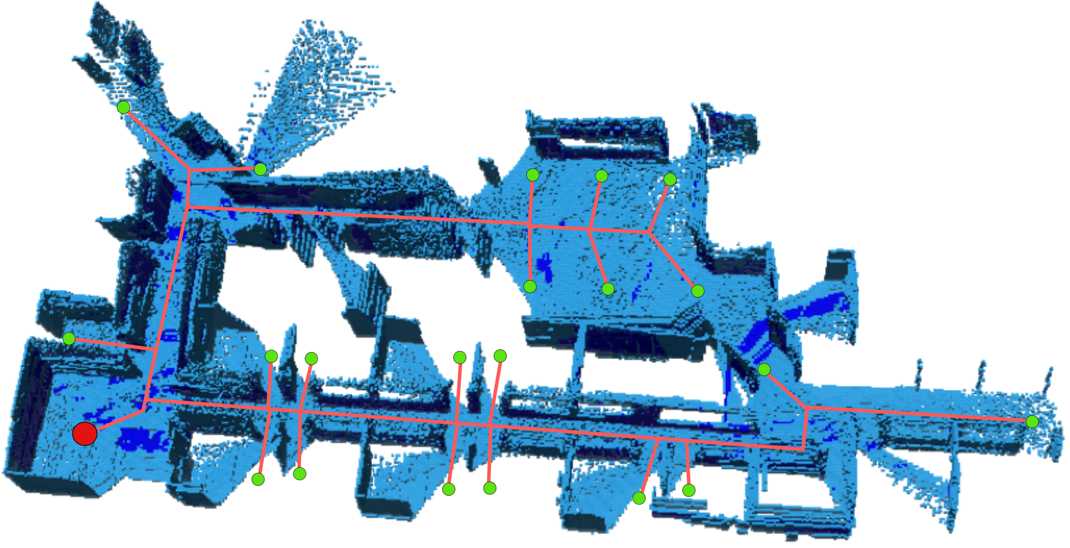
(a)

Figure 1: Illustration of possible candidate actions during exploration of an unknown environment by an autonomous robot. Robot’s current position is marked by red circle; red lines and green points represent trajectory and final position of each candidate action respectively. As can be seen, actions share many mutual parts.

However, in many BSP applications candidate (non-myopic) actions are partially overlapping, i.e. have similar parts. For instance, in a building exploration scenario, candidate actions are trajectories to different locations in a building (see Figure 1) that were provided e.g. by sampling-based motion planning approaches; some of these sampled trajectories will have mutual parts. Typically, these common parts will be evaluated a number of times, as part of evaluation of each action that shares it. Given that we know what are the similar parts between the different candidate actions, it can significantly reduce runtime complexity if we could handle these similar parts only once.

In this paper we present a technique for computation re-use between the candidate actions and exploitation of actions’ similarity, while leveraging the above-mentioned method for incremental covariance updates. We show that such a technique greatly reduces the total decision making runtime. Moreover, we argue that for most cases, explicit inference over the posterior belief is not required and that computation of the objective function can be done efficiently with complexity that is independent of state dimension. In general, the objective function of BSP can contain multiple terms, such as control cost, distance to goal and an information-theoretic term (e.g. entropy, information gain or mutual information). Arguably, in typical settings the control cost and distance to goal can be calculated without explicit inference over the posterior belief, since these terms depend only on linearization point of the state vector. In this paper we show that also the information term does not require an explicit inference over the posterior belief and that action similarity can be efficiently exploited, concluding that BSP problem can be solved without performing time-consuming explicit inference over the posterior belief at all.

To that end, we present a new paradigm that represents all candidate (sequence of) actions in a single unified data structure that allows to exploit the similarities between candidate actions while evaluating the impact of each such action. We refer to this structure as factor-graph propagation (FGP) action tree, and show that the developed herein incremental covariance calculation method allows us to compute information gain of the tree’s various parts. This, in turn, can be used to efficiently evaluate the information term of different candidate actions while re-using calculations when possible. Combining our recently-developed rAMDL approach (Kopitkov and Indelman, 2017) with factor-graph propagation (FGP) action tree and incremental covariance update, yields an approach that calculates action impact without explicitly performing inference over the posterior belief, while re-using calculations among different candidate actions.

To summarize, our main contributions in this paper are as follows: (a) we develop an incremental covariance update method to calculate specific covariance entries after any change in inference problem; (b) we present factor-graph propagation (FGP) action tree, that represents all candidate actions in single hierarchical model and allows to formulate mutual parts of the actions as a single sub-actions; (c) we apply incremental covariance update method to calculate covariance entries from intermediate and posterior beliefs within the FGP action tree, with complexity independent of state dimension; and (d) we combine the FGP action tree graphical model, the incremental covariance update method and rAMDL approach (Kopitkov and Indelman, 2017) to yield a new algorithm rAMDL-Tree that efficiently solves an information-theoretic BSP problem while handling candidates’ mutual parts only once.

This paper is organized as following. In Section 2 we describe the relevant work done in this field. Section 3 contains preliminaries and problem definition. In Section 4, we describe our approaches for incremental covariance recovery (Section 4.1) and information-theoretic BSP problem (Section 4.2). Further, in Section 5 we provide our simulation results that emphasize advantages of the presented herein approaches. Finally, in Section 6 we conclude the discussion about the introduced methods and point out several directions for future research. Additionally, at the end of this paper there is an appendix where we put proofs of several lemmas to improve readability.

2 Related Work

In this section we discuss the most relevant work to our approach, starting with computationally efficient covariance calculation and then proceeding to state of the art belief space planning approaches.

Computationally Efficient Covariance Recovery in High-Dimensional State Spaces

Fast covariance recovery, under the Gaussian inference setting, is an active research area that has been addressed by several works in the recent years. Naïvely calculating an inverse of a high-dimensional information matrix is prohibitively expensive. However, these calculations can be avoided by exploiting sparsity of the square root information matrix, yielding a recursive method to calculate the required entries (Golub and Plemmons, 1980), which has been recently also proposed by Kaess and Dellaert (Kaess and Dellaert, 2009) within their incremental smoothing and mapping solver. Although such method is faster than a simple inverse of square-root information matrix, the covariances are still calculated from scratch and the complexity depends on state dimension $n$. Moreover, in order to calculate a specific block of covariance matrix, the recursive approach may still need to calculate the entire covariance matrix (with dimensions $n\times n$) which is very undesirable for high-dimensional state spaces.

More recently, Ila et al. (Ila et al., 2015) introduced an approach to incrementally update covariances after the inference problem was changed. Given specific prior covariance entries that were calculated in previous timestep, their approach efficiently calculates covariance deltas to these entries, which comes out to be much faster than the recursive approach from (Kaess and Dellaert, 2009). Although this approach is similar in spirit to our method of incremental covariance update, it is more limited in the following sense. Its theoretical part deals only with the specific scenario where new observations were introduced to the inference problem, without adding new variables. On the other hand, the mathematical formulation of their approach does not handle the common scenario where the state vector is augmented with new variables, although the simulation part of (Ila et al., 2015) suggests that their approach can also be applicable in this case in practice. We emphasize that this approach is not mathematically sound in the state augmentation case, since such a case involves singular matrices that are assumed to be invertible according to the derivation of (Ila et al., 2015). Moreover, in case of state relinearization, the authors use a recursive method as fallback and calculate covariances from scratch. In contrast, we present a general approach that is mathematically sound and is capable of dealing with any change in the inference problem, including state augmentation and relinearization. Moreover, even though a limited version of incremental covariance update has been developed (Ila et al., 2015), it was not considered within a BSP problem, which is one of our main contributions in this work.

Belief Space Planning

As was mentioned above, BSP is an instantiation of a POMDP problem. Optimal solution of POMDP is known to be intractable (Kaelbling et al., 1998) in high-dimensional domains due to curse of dimensionality. Therefore, most of the modern research is focused on approximation methods that solve the planning problem in sub-optimal form with tractable runtime complexity. These approximation methods can be categorized into those that discretize the state/action/measurement space domains and those that act in continuous spaces. Approaches that perform discretization include sampling (Prentice and Roy, 2009; Agha-Mohammadi et al., 2014), simulation (Stachniss et al., 2005) and point-based value iteration (Pineau et al., 2006) methods. Planning approaches that operate in continuous spaces, often also termed as direct trajectory optimization methods, calculate a locally optimal solution given an initial nominal solution using different optimization techniques such as dynamic programming and gradient descent (Indelman et al., 2015; Van Den Berg et al., 2012; Patil et al., 2014; Platt et al., 2010).

Additionally, BSP methods can be separated into those that solve myopic and non-myopic decision making. While myopic approaches, also known as next best view (NBV) approaches in computer vision community (e.g. (Wenhardt et al., 2007; Dunn and Frahm, 2009)), reason about actions taking the system only one step into the future, non-myopic planning (e.g. (Platt et al., 2010; He et al., 2011; Van Den Berg et al., 2012; Kim and Eustice, 2014; Indelman et al., 2015)) deals with sequences of actions taking the system multiple steps into the future. Clearly, for more complex tasks non-myopic methods will perform better as the time period before receiving the reward can be long. Yet, such methods are typically more computationally expensive as more effort is required to consider different probabilistic outcomes along the long planning horizon. In this paper we consider a non-myopic setting and formulate the problem through factor graphs.

An information-theoretic BSP problem seeks for an optimal action that maximally reduces estimation uncertainty of the state vector. Such a problem can be separated into two main cases - unfocused BSP tries to reduce uncertainty of all variables inside the state vector, whereas focused BSP is only interested to reduce uncertainty of a predefined subset (termed as focused variables) of these variables. Typically, the two cases have different best actions, with optimal action from unfocused BSP potentially providing little information about focused variables of focused BSP (see e.g. (Levine and How, 2013)). In both cases, the objective function usually calculates posterior entropy or information gain (of all variables from the state vector or of only focused variables) and may have high computation complexity that depends on state dimension $n$. For instance, the calculation of unfocused posterior entropy usually requires determinant computation of information (covariance) matrix which is in general $O(n^{3})$, and is smaller for sparse matrices as in SLAM problems (Bai et al., 1996). Calculation of focused posterior entropy is even more expensive and requires additional Schur complement computation.

Recently, we presented a novel approach, rAMDL (Kopitkov and Indelman, 2017), to efficiently calculate entropy and information gain for both focused and unfocused cases. This method requires only one-time calculation that depends on dimension $n$ - computation of specific prior marginal (or conditional) covariances. Given these prior covariances, rAMDL evaluates information impact of each candidate action independently of state dimension $n$. Such a technique was shown to significantly reduce runtime (by orders of magnitude) compared to standard approaches.

Yet, in most BSP approaches, including our own rAMDL approach, the similarity between candidate actions is not exploited and each candidate is evaluated from scratch. To the best of our knowledge, only the work by Chaves et al. (Chaves and Eustice, 2016) was done in this direction. Their approach performs fast explicit inference over the posterior belief, by constraining variable ordering of the Bayes tree data structure to have candidates’ common variables eliminated first. Still, this approach has its limitations. It explicitly calculates the posterior belief for each action, and though it is done fast, it still requires additional memory to store such posterior beliefs. Further, it does not deal with information-theoretic objective functions whose runtime complexity is usually very expensive, as mentioned above. Moreover, it can only be applied when the SLAM algorithm is implemented using Bayes tree (Kaess et al., 2012), and it was shown to work only for the case where actions are trajectories constrained to have only a single common part.

In contrast, in this paper we develop a BSP technique that re-uses calculations in a general way, by exploiting potentially any number of mutual parts between the candidate actions. It is expressed in terms of factor graphs and can be applied not just for trajectory planning, but for any decision making problem expressed via factor graphs. Moreover, our technique can be implemented independently of a chosen SLAM factor graph optimization infrastructure. We combine several algorithmic concepts together - a unified graphical model FGP action tree, incremental covariance update and rAMDL approach (Kopitkov and Indelman, 2017), and present a BSP solution that does not require explicit inference over the posterior belief while carefully evaluating information impact of each action in an exact way.

3 Notations and Problem Formulation

Notation	Description
$X_{-}$	Problem 1: state vector before a change in inference problem;
	Problem 2: state vector at planning time
$X_{+}$	Problem 1: state vector after a change in inference problem;
	Problem 2: future state vector after applying a specific candidate action
$X_{new}$	Problem 1: new state variables introduced after a change in inference problem;
	Problem 2: new state variables introduced after applying a specific candidate action
$F_{new}$	Problem 1: new factors set introduced after a change in inference problem;
	Problem 2: new factors set introduced after applying a specific candidate action
$\Lambda_{-}$ and $\Lambda_{+}$	prior and posterior information matrices
$\Lambda_{+}^{Aug}$	prior information matrix $\Lambda_{-}$ augmented with zero rows and columns
	that represent new state variables $X_{new}$ (see Figure 3)
$\Sigma_{-}$ and $\Sigma_{+}$	prior and posterior covariance matrices
$R_{-}$ and $R_{+}$	prior and posterior square-root information upper-triangular matrices
$b[X]$	belief of state vector $X$
$\mathcal{H}(b[X])$	differential entropy of belief $b[X]$
$\Sigma^{M,Y}$	marginal covariance of some state subset $Y$
	(partition of covariance matrix $\Sigma$ with columns$\backslash$rows belonging to $Y$)
$I(a)$	increment of candidate action $a$, represents new factors and new state variables
	introduced into inference problem after $a$ is executed
$\mathcal{A}$	set of candidate actions considered in BSP
$A$	noise-weighted Jacobian of newly introduced factors w.r.t. all state variables

Table 1: Main notations used within problem definition (Section 3).

Consider a high-dimensional problem-specific state vector $X_{-}\in\mathbb{R}^{n}$ at the current time, where we use the notation ”-” to represent the (a priori) state vector before applying the next action. Depending on the application, $X_{-}$ can represent robot configuration and poses (optionally also past and current poses), environment-related variables or any other variables of interest. Additionally, consider factors $F=\{f^{1}(X^{1}),\ldots,f^{n_{f}}(X^{n_{f}})\}$ that were added to the inference problem till (and including) current time, where each factor $f^{j}(X^{j})$ represents a specific measurement model, motion model or prior, and as such involves appropriate state variables $X^{j}\subseteq X_{-}$.

The joint pdf (probability density function) can be then written as

$$\mathbb{P}({X_{-}|history})\propto\prod_{j=1}^{n_{f}}f^{j}(X^{j}),$$ (1)

where $history$ contains all the information gathered by the current time (measurements, controls, etc.).

As common in many inference problems, we will assume that all factors have a Gaussian form:

$$f^{j}(X^{j})\propto\exp(-\frac{1}{2}\|h^{j}(X^{j})-r^{j}\|_{\Sigma^{j}}^{2}),$$ (2)

with appropriate model

$$r^{j}=h^{j}(X^{j})+\upsilon^{j},\quad\upsilon^{j}\sim\mathcal{N}(0,\Sigma^{j}),$$ (3)

where $h^{j}$ is a known nonlinear function, $\upsilon^{j}$ is zero-mean Gaussian noise and $r^{j}$ is the expected value of $h^{j}$, i.e. $r^{j}=\mathbb{E}[h^{j}(X^{j})]$. Such a factor representation is a general way to express information about the state. In particular, it can represent a measurement model, in which case, $h^{j}$ is the observation model, and $r^{j}$ and $\upsilon^{j}$ are, respectively, the actual measurement $z$ and measurement noise. Similarly, it can also represent a motion model. A maximum a posteriori (MAP) inference is the optimization solution of maximizing Eq. (1) w.r.t. state $X_{-}$. It can be efficiently calculated (see e.g. Kaess et al. (2012)) such that

$$\mathbb{P}({X_{-}|history})=\mathcal{N}(X_{-}^{\star},\Sigma_{-})=\mathcal{N}^{-1}(\eta_{-}^{\star},\Lambda_{-})$$ (4)

where $X^{\star}_{-}$, $\Sigma_{-}$, $\eta^{\star}_{-}$ and $\Lambda_{-}$ are respectively the current mean vector, covariance matrix, information vector and information matrix (inverse of covariance matrix).

We shall refer to the belief $\mathbb{P}({X_{-}|history})$ of state $X_{-}$ at the current time as the prior belief and write

$$b[X_{-}]\doteq\mathbb{P}({X_{-}|history}).$$ (5)

We now introduce the two problems this paper addresses, along with appropriate notations: general purpose incremental covariance update, and computationally efficient belief space planning. As will be seen in Section 4, our approach to address the latter problem builds upon the solution to the first problem.

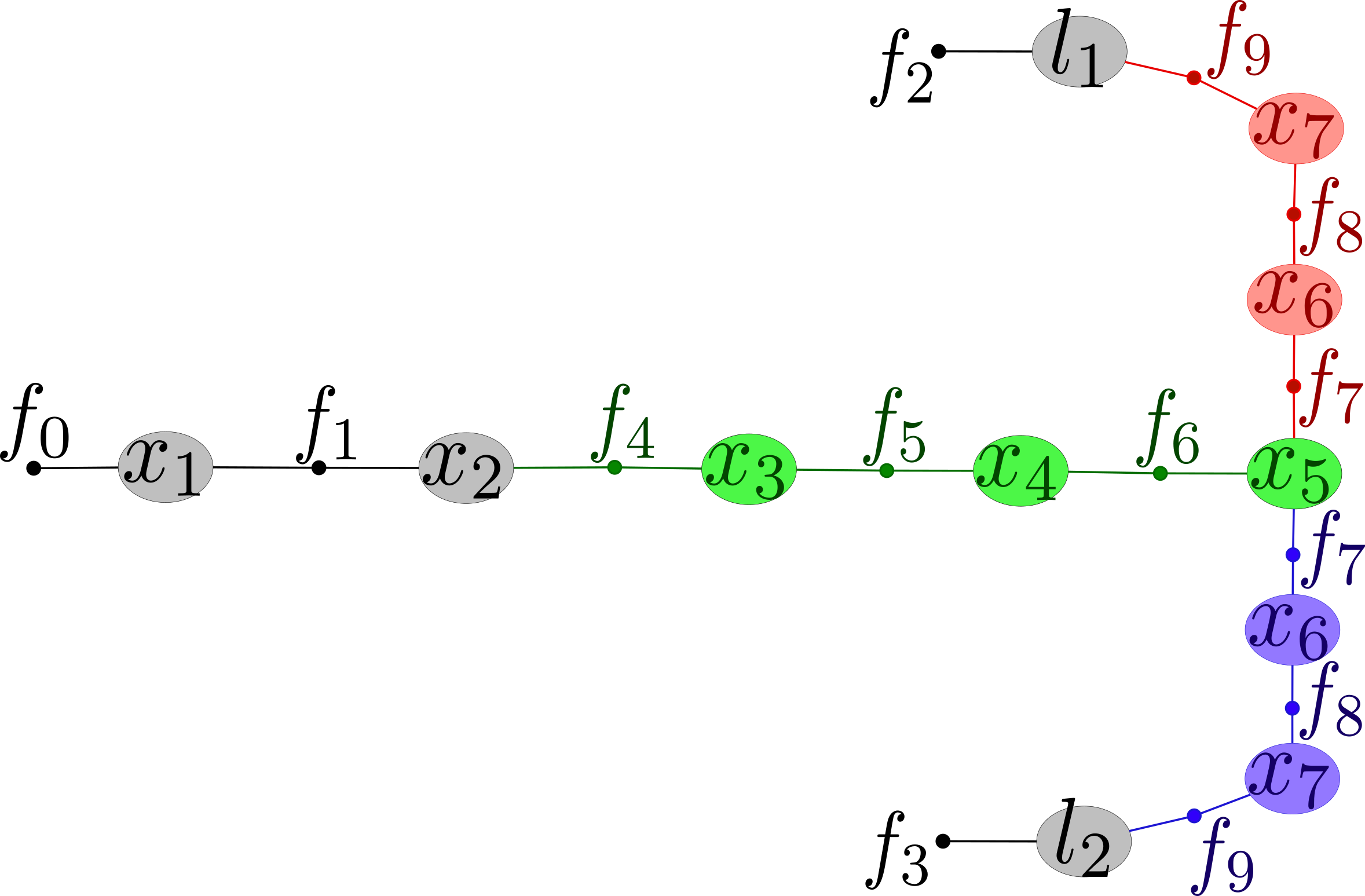
(a)

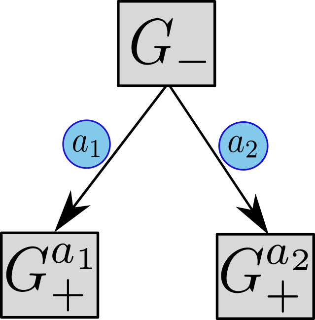
(b)

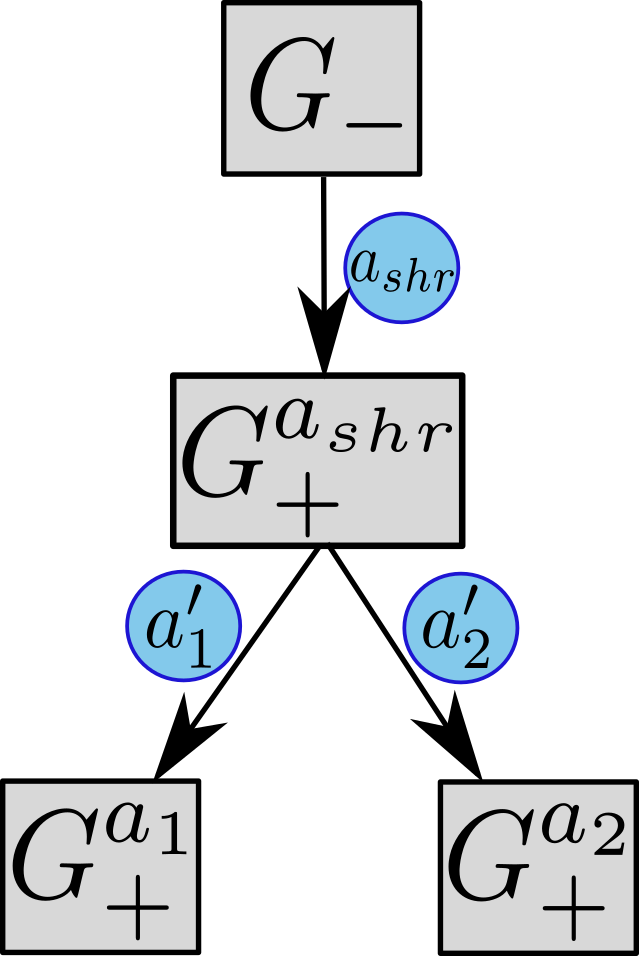
(c)

Figure 2: Illustration of belief propagation in factor graph representation, taken from SLAM application. (a) Prior factor graph $G_{-}$ (colored in black) contains two robot poses $x_{1}$ and $x_{2}$, and two landmarks $l_{1}$ and $l_{2}$, as also the prior and motion model factors $\{f_{0},f_{1},f_{2},f_{3}\}$. Two different actions (trajectories) are considered. The first will take the robot to observe landmark $l_{1}$ and will augment the $G_{-}$ with new factors and state variables colored in green and red. The second will take robot to visit $l_{2}$ instead, and will augment the $G_{-}$ with new factors and state variables colored in green and purple. As can be seen, both candidate actions are sharing some of their new factors/state variables (colored in green). (b)-(c) Candidates from (a) represented as FGP action tree. In FGP action tree each vertex represents a specific factor graph (or the belief that is associated with it) and each edge represents a specific action - augmentation of the factor graph with an increment of the action, see Eq. (10). (b): posterior factor graphs $G_{+}^{a_{1}}$ and $G_{+}^{a_{2}}$ are propagated separately for each action. (c): first the prior factor $G_{-}$ is augmented by a mutual increment represented by $a_{shr}$ (colored green in (a)) and the posterior $G_{+}^{a_{shr}}$ is received. Next, $G_{+}^{a_{shr}}$ is augmented separately by not-mutual increments (colored red and purple in (a)) of each action, providing posterior factor graphs $G_{+}^{a_{1}}$ and $G_{+}^{a_{2}}$.

Problem 1: Covariance Recovery

As mentioned above, in many applications it is mandatory to recover covariance entries of belief $b[X_{-}]$. However, typically this belief is represented through its information form ($\eta_{-}^{\star}$ and $\Lambda_{-}$), or the square-root information upper-triangular matrix $R_{-}$, with $\Lambda_{-}=R_{-}^{T}\cdot R_{-}$.

Considering a square-root representation, the covariance matrix is $\Sigma_{-}=R_{-}^{-1}\cdot R_{-}^{-T}$ and its specific covariance entries $\Sigma_{-}=(\sigma_{ij})$ can be calculated from entries $R_{-}=(r_{ij})$ as (Golub and Plemmons, 1980)

$$\sigma_{ii}=\frac{1}{r_{ii}}\Bigg{(}\frac{1}{r_{ii}}-\sum_{j=i+1,r_{ij}\neq 0}^{n}r_{ij}\sigma_{ji}\Bigg{)},$$ (6)

$$\sigma_{ij}=\frac{1}{r_{ii}}\Bigg{(}-\sum_{k=i+1,r_{ik}\neq 0}^{j}r_{ik}\sigma_{kj}-\sum_{k=j+1,r_{ik}\neq 0}^{n}r_{ik}\sigma_{kj}\Bigg{)}.$$ (7)

Note that in order to calculate the upper left covariance entry ($\sigma_{11}$), all other covariance entries are required. Therefore, worst case computation (and memory) complexity of this recursive approach is still quadratic in state dimension $n$.

In contrast, an incremental covariance update approach can be applied in order to recover the required covariance entries more efficiently. At each timestep, solving the inference problem for the current belief $b[X_{-}]$ from Eq. (1) provides MAP estimate and the corresponding covariance or (square root) information matrix. However, at the next step the inference problem changes. To see that, consider the belief at the next timestep $b[X_{+}]$ which was obtained by introducing new state variables $X_{new}$ (e.g. new robot poses in SLAM smoothing formulation), with $X_{+}=X_{-}\cup X_{new}$, and by adding new factors (e.g. new measurements, odometry, etc.) $F_{new}=\{f_{new}^{1}(X_{+}^{1}),\ldots,f_{new}^{n_{new}}(X_{+}^{n_{new}})\}$ where $X_{+}^{j}\subseteq X_{+}$. Additionally, consider the set of variables $Y\subset X_{+}$ whose marginal covariance $\Sigma_{+}^{M,Y}$ from $b[X_{+}]$ we are interested in calculating. Note that these variables of interest can contain both old $Y_{old}\subset X_{-}$ and new $Y_{new}\subset X_{new}$ variables, with $Y=\{Y_{old},Y_{new}\}$.

Given that we already calculated the required covariance entries $\Sigma_{-}^{M,Y_{old}}$ from the current belief $b[X_{-}]$, in incremental covariance update approach we would like to update these entries after the change in the inference problem (from $b[X_{-}]$ to $b[X_{+}]$) as:

$$\Sigma_{+}^{M,Y_{old}}=\Sigma_{-}^{M,Y_{old}}+\Delta^{Y_{old}},$$ (8)

where $\Delta^{Y_{old}}$ represents the difference between old and new covariance entries. Additionally, in the general case we might be interested in calculating the posterior covariance of new variables of interest $Y_{new}\subset Y$, i.e.  $\Sigma_{+}^{M,Y_{new}}$, as well as also the cross-covariances between $Y_{old}$ and $Y_{new}$.

Likewise, also the conditional covariances, from the conditional pdf of one state subset conditioned on another, are required for information-theoretic BSP as was shown in (Kopitkov and Indelman, 2017). Hence, we would also like to develop a similar approach for incremental conditional covariance update.

A limited technique to perform an incremental update of marginal covariances was presented in (Ila et al., 2015). The authors show how to update the covariance entries by downdating the posterior information matrix. Their derivation can be applied for the case where the state vector was not augmented during the change in the inference problem ($X_{new}$ is empty). However, that derivation is not valid for the case of state augmentation, which involves zero-padding of prior matrices (described below); such padding yields singular matrices and requires a more delicate handling. Even though their approach is not mathematically sound for the augmentation case, in the simulation part of (Ila et al., 2015) it is insinuated that the approach can also be applied here in practice. Still, the authors clearly declare that their approach does not handle relinearization of the state vector, which can often happen during the change in the inference problem. Further, (Ila et al., 2015) does not consider recovery of conditional covariances. In contrast, we develop a general purpose method that handles incremental (marginal and conditional) covariance updates in all of the above cases in a mathematically sound way.

In Section 4 we categorize the above general change in the inference problem into different sub-cases. Further, we present an approach that carefully handles each such sub-case and incrementally updates covariances that were already calculated before the change in the inference problem, and also computes covariance of newly introduced state variables. As will be shown, the computational complexity of such a method, when applied to a problem where only the marginal covariances need to be recovered (i.e. block diagonal of $\Sigma_{-}$), is linear in $n$ in the worst case. Furthermore, we will show how our incremental covariance update approach can be also applied to incrementally update conditional covariance entries. Later, this capability will be an essential part in the derivation of our BSP method, rAMDL-Tree.

Problem 2: Belief Space Planning

Typically in BSP and decision making problems we have a set of candidate actions $\mathcal{A}=\{a_{1},a_{2},...\}$ from which we need to pick the best action according to a given objective function. As shown in our previous work (Kopitkov and Indelman, 2017), the posterior belief for each action can be viewed as a specific augmentation of the prior factor graph that represents the prior belief $b[X_{-}]$ (see Figure 2a). In this paper we shall denote this factor graph by $G_{-}$. Each candidate action $a$ can add new information about the state variables in form of new factors. Additionally, in specific applications, action $a$ can also introduce new state variables into the factor graph (e.g. new robot poses). Thus, similarly to change in inference problem described above for each action $a$ we can model the newly introduced state variables denoted by $X_{new}$, defining the posterior state vector (after applying the action) as $X_{+}=X_{-}\cup X_{new}$. In a like manner, we denote the newly introduced factors by $F_{new}=\{f_{new}^{1}(X_{+}^{1}),\ldots,f_{new}^{n_{new}}(X_{+}^{n_{new}})\}$ where $X_{+}^{j}\subseteq X_{+}$.

Therefore, similar to Eq. (1), after applying candidate action $a$, the posterior belief $b[X_{+}]$ can be explicitly written as

$$b[X_{+}]\propto b[X_{-}]\prod_{j=1}^{n_{new}}f_{new}^{j}(X_{+}^{j}).$$ (9)

Such a formulation is general and supports non-myopic action $a$ with any planning horizon, that introduces into the factor graph multiple new state variables and multiple factors with any measurement model. Still, in this paper we assume factors to have a Gaussian form (Eq. (2)).

For the sake of conciseness, in this paper the newly introduced factors and state variables that are added when considering action $a$ will be called action $a$’s increment and denoted as

$$I(a)\doteq\{F_{new},X_{new}\}$$ (10)

The posterior information matrix, i.e. the second moment of the belief $b[X_{+}]$, can be written as

$$\Lambda_{+}=\Lambda_{-}+A^{T}\cdot A\quad,\quad\Lambda_{+}=\Lambda_{+}^{Aug}+A^{T}\cdot A$$ (11)

where we took the maximum likelihood assumption which considers that the above, a single optimization iteration (e.g. Gauss Newton), sufficiently captures action impact on the belief. Such an assumption is typical in BSP literature (see, e.g. (Platt et al., 2010; Van Den Berg et al., 2012; Kim and Eustice, 2014; Indelman et al., 2015)). The left identity in Eq. (11) is true when $X_{new}$ is empty, while the right identity is valid for non-empty $X_{new}$. The matrix $A$ is a noise-weighted Jacobian of newly introduced factors $F_{new}$ w.r.t. state variables $X_{+}$; $\Lambda_{+}^{Aug}$ is constructed by first augmenting the prior information matrix $\Lambda_{-}$ with zero rows and columns representing the new state variables $X_{new}$, as illustrated in Figure 3 (see e.g. (Kopitkov and Indelman, 2017)).

(a)

Figure 3: Illustration of $\Lambda_{+}$’s construction for a given candidate action in case new state variables $X_{new}$ were introduced into the state vector. First, $\Lambda_{+}^{Aug}$ is created by adding zero rows and columns representing the new state variables. Then, the new information of belief is computed through $\Lambda_{+}=\Lambda_{+}^{Aug}+A^{T}A$.

After modeling the posterior information matrix $\Lambda_{+}$ for action $a$, the unfocused information gain (uncertainty reduction of the entire state vector $X_{+}$) can be computed as:

$$J_{IG}(a)=\mathcal{H}(b[X_{-}])-\mathcal{H}(b[X_{+}])=dim.const+\frac{1}{2}\ln\frac{\begin{vmatrix}\Lambda_{+}\end{vmatrix}}{\begin{vmatrix}\Lambda_{-}\end{vmatrix}}$$ (12)

where $\mathcal{H}(\cdot)$ is differential entropy function that measures the uncertainty of input belief, and $dim.const$ is a constant that only depends on the dimension of $X_{+}$ and thus is ignored in this paper. Note that the above unfocused information gain is typically used in applications where the set of new variables, $X_{new}$, is empty and so both $X_{-}$ and $X_{+}$ have the same dimension. In cases where $X_{new}$ is not empty (e.g. SLAM smoothing formulation), usually focused information gain is used (see below).

The optimal action $a^{*}$ is then given by $a^{*}=\operatorname*{arg\,max}_{a\in\mathcal{A}}J_{IG}(a)$.

For focused BSP problem we would like to reduce uncertainty of only a subset of state variables $X^{F}\subseteq X_{+}$. When $X^{F}$ consists of old variables $X_{-}$, $X^{F}\subseteq X_{-}$, we can compute its information gain (IG). Such IG is a reduction of $X^{F}$’s entropy after applying action $a$, $\mathcal{H}(b[X_{-}^{F}])-\mathcal{H}(b[X_{+}^{F}])$ where $b[X_{-}^{F}]$ and $b[X_{+}^{F}]$ are prior and posterior beliefs of focused variables $X^{F}$. In case $X^{F}$ consists of newly introduced variables $X_{new}$, $X^{F}\subseteq X_{new}$, the IG function has no meaning as the prior belief $b[X_{-}^{F}]$ does not exist. Instead, we can directly calculate $X^{F}$’s posterior entropy $\mathcal{H}(b[X_{+}^{F}])$. The IG and entropy functions can be calculated through respectively:

$$J_{IG}^{F}(a)=\frac{1}{2}\ln\frac{\begin{vmatrix}\Sigma_{-}^{M,F}\end{vmatrix}}{\begin{vmatrix}\Sigma_{+}^{M,F}\end{vmatrix}},\quad J_{\mathcal{H}}^{F}(a)=dim.const+\frac{1}{2}\ln\begin{vmatrix}\Sigma_{+}^{M,F}\end{vmatrix},$$ (13)

where $\Sigma_{-}^{M,F}$ and $\Sigma_{+}^{M,F}$ are prior and posterior marginal covariance matrices of $X^{F}$, respectively. Note that in focused BSP the optimal action will be found through $a^{*}=\operatorname*{arg\,max}_{a\in\mathcal{A}}J_{IG}^{F}(a)$ or $a^{*}=\operatorname*{arg\,min}_{a\in\mathcal{A}}J_{\mathcal{H}}^{F}(a)$.

To summarize, in order to solve an information-theoretic BSP problem, we are required to calculate IG or entropy (Eqs. (12) and (13)) for each candidate action $a$, and then choose a candidate action with the maximal gain.

4 Approach

In this section we present our approaches that efficiently solve the incremental covariance recovery (Section 4.1) and information-theoretic BSP (Section 4.2).

4.1 Incremental Covariance Update

In this section we present our technique for efficient update of covariance entries (see Problem 1 in Section 3). In Section 4.1.1 we show how to update marginal covariances of specified variables $Y\subset X_{+}$ after new state variables were introduced into the state vector and new factors were added, yet no state relinearization happened during the change in the inference problem. We will show that the information matrix of the entire state belief is propagated through quadratic update form, similarly to Eq. (11). Assuming such quadratic update, we will derive a method to efficiently calculate the change in old covariance entries, to compute the new covariance entries and the cross-covariances between old and new state variables. Further, in Section 4.1.2 we will show that also in the relinearization case the information matrix update has an identical quadratic update form and conclude that our method, derived in Section 4.1.1, can also be applied when some of the state variables were relinearized. Finally, in Section 4.1.3 we will show that also the information matrix of a conditional pdf is updated through quadratic update form and that the same technique from Section 4.1.1 can be applied in order to incrementally update conditional covariance entries. We will show that our approach’s complexity, given the specific prior covariances, does not depend on state dimension $n$.

4.1.1 Update of Marginal Covariance Entries

Notation	Description
$Y$	subset of state variables whose marginal covariance we are interested to update$\backslash$compute
$Y_{old}$	old variables inside $Y$
$Y_{new}$	new variables inside $Y$ (that were introduced during the change in the inference problem)
${}^{I}\!X$	set of old involved variables in the newly introduced factors $F_{new}$
$W$	variable union of sets $Y_{old}$ and ${}^{I}\!X$
$n$	dimension of a prior state vector $X_{-}$
$N$	dimension of a posterior state vector $X_{+}$
$m$	overall dimension of the newly introduced factors $F_{new}$
${}^{I}\!A$	$m\times|{}^{I}\!X|$ matrix that consists of $A$’s columns belonging to variables in ${}^{I}\!X$

Table 2: Main notations used through derivation of incremental covariance recovery approach.

Consider Problem 1 from Section 3. Consider the belief was propagated from $b[X_{-}]$ to $b[X_{+}]$ as described. Yet, let us assume for now that no state relinearization happened (we will specifically handle it in the next section). In this section we show that the posterior covariances of interest $\Sigma_{+}^{M,Y}$ can be efficiently calculated as

$$\Sigma_{+}^{M,Y}=f(\Sigma_{-}^{M,W}),$$ (14)

where $\Sigma_{-}^{M,W}$ is the prior marginal covariance of set $W\doteq\{Y_{old},{}^{I}\!X\}$ and $f(\cdot)$ is a transformation function, with calculation complexity that does not depend on state dimension $n$. We derive this function in detail below. The set $Y_{old}$ contains old state variables inside $Y$ ($Y_{old}\subseteq X_{-}$) and ${}^{I}\!X\subseteq X_{-}$ is the set of involved variables in the newly introduced factors $F_{new}$ - variables that appear in $F_{new}$’s models (Eq. (3)). Note that the update of old covariances (Eq. (8)) is only one part of this $f(\cdot)$, as also the computation of covariances for new state variables $Y_{new}$ and cross-covariances between $Y_{old}$ and $Y_{new}$.

Next, let us separate all possible changes in the inference problem into different cases according to augmented state variables $X_{new}$ and the newly introduced factors $F_{new}$.

If $X_{new}$ is empty, we will call such a case as not-augmented. This case does not change the state vector ($X_{-}\equiv X_{+}$) and only introduces new information through new factors. The information matrix in this case can be updated through $\Lambda_{+}=\Lambda_{-}+A^{T}\cdot A$, where matrix $A\in\mathbb{R}^{m\times n}$ is a noise-weighted Jacobian of newly introduced factors $F_{new}$ w.r.t. state variables $X_{+}$, and $A$’s height $m$ is dimension of all new factors within $F_{new}$ (see Section 3).

Given $X_{new}$ is not empty, we will call such a case as rectangular. This case augments the state vector to be $X_{+}=\{X_{-},X_{new}\}$ and also introduces new information through the new factors. Here the information matrix can be updated through $\Lambda_{+}=\Lambda_{+}^{Aug}+A^{T}\cdot A$ where $\Lambda_{+}^{Aug}\in\mathbb{R}^{N\times N}$ is a singular matrix that is constructed by first augmenting the prior information matrix $\Lambda_{-}$ with zero rows and columns representing the new state variables $X_{new}$, as illustrated in Figure 3; $N=|X_{+}|=n+|X_{new}|$ is the posterior state dimension; $A$ here will be an $m\times N$ matrix.

Finally, for the case when $X_{new}$ is not empty and total dimension of new factors $m$ is equal to the number of newly introduced variables $|X_{new}|$, we will call such a case as squared. Clearly, the squared case is a specific case of the rectangular case, which for instance can represent the new robot poses of candidate trajectory and the new motion model factors. The reason for this specific case to be dealt with in special way is due to the fact that its $f(\cdot)$ function is much simpler than $f(\cdot)$ function of the more general rectangular case, as we will show below. Thus, when $m=|X_{new}|$ it would be advisable to use function $f(\cdot)$ of the squared case.

The summery of the above cases can be found in Table 3.

Case	$\mathbf{X_{new}}$	Information	Posterior State	$\mathbf{A}$’s Dimension
		Update	Dimension
Not-augmented	empty	$\Lambda_{+}=\Lambda_{-}+A^{T}\cdot A$	$n$	$m\times n$
Rectangular	not empty	$\Lambda_{+}=\Lambda_{+}^{Aug}+A^{T}\cdot A$	$N=n+|X_{new}|$	$m\times N$
Squared (subcase of Rectangular)	not empty	$\Lambda_{+}=\Lambda_{+}^{Aug}+A^{T}\cdot A$	$N=n+|X_{new}|$	$m\times N$, $m=|X_{new}|$

Table 3: Summery of all different variations of change in inference problem. We use $n$ to denote prior state dimension; $N$ - posterior state dimension; $m$ - dimension of all new factors within $F_{new}$.

Next, below we present the function $f(\cdot)$ separately for each one of the not-augmented, rectangular and squared cases. Although the function $f(\cdot)$ has an intricate form (especially in the rectangular case), all matrix terms involved in it have dimensions $m$, $|X_{new}|$ or $|{}^{I}\!X|$; hence, overall calculation of posterior $\Sigma_{+}^{M,Y}$ does not depend on state dimension $n$.

Lemma 1

For the not-augmented case, the posterior marginal covariance $\Sigma_{+}^{M,Y}$ can be calculated as:

$$\Sigma_{+}^{M,Y}=\Sigma_{-}^{Y}-B\cdot C^{-1}\cdot B^{T},\quad B\triangleq\Sigma_{-}^{C}\cdot({}^{I}\!A)^{T},\quad C\triangleq I_{m}+{}^{I}\!A\cdot\Sigma_{-}^{I}\cdot({}^{I}\!A)^{T}$$ (15)

where $\Sigma_{-}^{I}$, $\Sigma_{-}^{Y}$ and $\Sigma_{-}^{C}$ are parts of prior marginal covariance $\Sigma_{-}^{M,W}$ partitioned through $W=\{Y,{}^{I}\!X\}$:

$$\Sigma_{-}^{M,W}=\begin{pmatrix}\Sigma_{-}^{Y}&\Sigma_{-}^{C}\\ (\Sigma_{-}^{C})^{T}&\Sigma_{-}^{I}\\ \end{pmatrix}$$ (16)

and where ${}^{I}\!A$ consists of $A$’s columns belonging to involved old variables ${}^{I}\!X$.

The proof of Lemma 1 is given in Appendix 7.1. Note that sets $Y$ and ${}^{I}\!X$ are not always disjoint. In case these sets have mutual variables, the cross-covariance matrix $\Sigma_{-}^{C}$ can be seen just as $\Sigma_{-}^{(Y,{}^{I}\!X)}$ - partition of prior covariance matrix $\Sigma_{-}$ with rows belonging to $Y$ and columns belonging to ${}^{I}\!X$.

Lemma 2

For the rectangular case the prior marginal covariance $\Sigma_{-}^{M,W}$ and the posterior marginal covariance $\Sigma_{+}^{M,Y}$ have the forms:

$$\Sigma_{-}^{M,W}=\begin{pmatrix}\Sigma_{-}^{Y_{old}}&\Sigma_{-}^{C}\\ (\Sigma_{-}^{C})^{T}&\Sigma_{-}^{I}\\ \end{pmatrix}$$ (17)

$$\Sigma_{+}^{M,Y}=\begin{pmatrix}\Sigma_{+}^{M,Y_{old}}&\Sigma_{+}^{(Y_{old},Y_{new})}\\ (\Sigma_{+}^{(Y_{old},Y_{new})})^{T}&\Sigma_{+}^{M,Y_{new}}\\ \end{pmatrix}$$ (18)

where we partition $Y$ variables into two subsets $Y_{old}\doteq X_{-}\cap Y$ and $Y_{new}\doteq X_{new}\cap Y$, and where $W=\{Y_{old},{}^{I}\!X\}$.

Using parts of $\Sigma_{-}^{M,W}$ we can calculate parts of $\Sigma_{+}^{M,Y}$ as:

$$\Sigma_{+}^{M,Y_{old}}=\Sigma_{-}^{Y_{old}}-B\cdot G^{-1}\cdot B^{T}$$ (19)

$$\Sigma_{+}^{M,Y_{new}}=P^{(Y_{new},:)}$$ (20)

$$C\triangleq I_{m}+{}^{I}\!A\cdot\Sigma_{-}^{I}\cdot({}^{I}\!A)^{T}$$ (21)

$$P\triangleq[(A_{new}^{T}\cdot C^{-1}\cdot A_{new})^{-1}]^{(:,Y_{new})}$$ (22)

$$F\triangleq(A_{new}^{T}\cdot A_{new})^{-1}$$ (23)

$$K\triangleq I_{m}-A_{new}\cdot F\cdot A_{new}^{T}$$ (24)

$$K_{1}\triangleq K\cdot{}^{I}\!A$$ (25)

$$B\triangleq\Sigma_{-}^{C}\cdot K_{1}^{T}$$ (26)

$$G\triangleq I_{m}+K_{1}\cdot\Sigma_{-}^{I}\cdot K_{1}^{T}$$ (27)

where $A_{new}$ consists of $A$’s columns belonging to newly introduced variables $X_{new}$. Also, we use matrix slicing operator (e.g. $P^{(Y_{new},:)}$) as it is accustomed in Matlab syntax.

Further, there are two methods to calculate $\Sigma_{+}^{(Y_{old},Y_{new})}$ from Eq. (18):

Method 1:

$$\Sigma_{+}^{(Y_{old},Y_{new})}=\Sigma_{-}^{C}\cdot({}^{I}\!A)^{T}\cdot[C^{-1}\cdot{}^{I}\!A\cdot\Sigma_{-}^{I}\cdot({}^{I}\!A)^{T}-I_{m}]\cdot A_{new}\cdot P$$ (28)

Method 2:

$$\Sigma_{+}^{(Y_{old},Y_{new})}=\Sigma_{-}^{C}\cdot[K_{1}^{T}\cdot G^{-1}\cdot K_{1}\cdot\Sigma_{-}^{I}-I_{k}]\cdot({}^{I}\!A)^{T}\cdot A_{new}\cdot F^{(:,Y_{new})}$$ (29)

Empirically we found that method 2 is the fastest option. The proof of Lemma 2 is given in Appendix 7.2.

Lemma 3

For the squared case the prior marginal covariance $\Sigma_{-}^{M,W}$ and the posterior marginal covariance $\Sigma_{+}^{M,Y}$ have the forms:

$$\Sigma_{-}^{M,W}=\begin{pmatrix}\Sigma_{-}^{Y_{old}}&\Sigma_{-}^{C}\\ (\Sigma_{-}^{C})^{T}&\Sigma_{-}^{I}\\ \end{pmatrix}$$ (30)

$$\Sigma_{+}^{M,Y}=\begin{pmatrix}\Sigma_{+}^{M,Y_{old}}&\Sigma_{+}^{(Y_{old},Y_{new})}\\ (\Sigma_{+}^{(Y_{old},Y_{new})})^{T}&\Sigma_{+}^{M,Y_{new}}\\ \end{pmatrix}$$ (31)

where we partition $Y$ variables into two subsets $Y_{old}\doteq X_{-}\cap Y$ and $Y_{new}\doteq X_{new}\cap Y$, and where $W=\{Y_{old},{}^{I}\!X\}$.

Using parts of $\Sigma_{-}^{M,W}$ we can calculate parts of $\Sigma_{+}^{M,Y}$ as:

$$\Sigma_{+}^{M,Y_{old}}=\Sigma_{-}^{Y_{old}}$$ (32)

$$\Sigma_{+}^{M,Y_{new}}=A_{iv}\cdot C\cdot A_{iv}^{T}$$ (33)

$$\Sigma_{+}^{(Y_{old},Y_{new})}=-\Sigma_{-}^{C}\cdot({}^{I}\!A)^{T}\cdot(A_{iv})^{T}$$ (34)

$$A_{iv}\triangleq[A_{new}^{-1}]^{(Y_{new},:)}$$ (35)

$$C\triangleq I_{m}+{}^{I}\!A\cdot\Sigma_{-}^{I}\cdot({}^{I}\!A)^{T}.$$ (36)

We can see that in case of a squared alteration, the covariances of old variables $X_{-}$ do not change. The proof of Lemma 3 is given in Appendix 7.3.

Note that in some applications the inner structure of Jacobian partitions ${}^{I}\!A$ and $A_{new}$ can be known a priori. In these cases such knowledge can be exploited and the runtime complexity of the above equations can be reduced even more.

4.1.2 Incremental Covariance Update After Relinearization

Till now we have explored scenarios where new information is introduced into our estimation system in a quadratic form via Eq. (11). Such information update is appropriate for planning problems where we take linearization point of existing variables $X_{-}$ (their current mean vector) and assume to know linearization point of newly introduced variables $X_{new}$. However, during the inference process itself, state relinearization can happen and such a quadratic update form is not valid anymore. This is because some factors, linearized with the old linearization point, are removed from the system and their relinearized versions are then introduced. In this case the derived approach to incrementally update posterior covariances cannot be used as it is. In this section we describe the alternative that can be applied after a relinearization event and which is more efficient than state-of-the-art approaches that calculate specific posterior covariances from posterior information matrix from scratch.

Relineariztion may happen when a significantly new information was added into the inference problem and current linearization point of state vector $X_{-}$ does not optimally explain it anymore. In such cases, iterative optimization algorithms, such as Gauss-Newton, are responsible to update the current linearization point, i.e. to find a more optimal linearization point that better explains the collected so far measurement/motion/prior factors. Conventional approaches re-linearize the entire state vector when new data comes in. On the other hand, incremental optimizer ISAM2 (Kaess et al., 2012) tracks instead the validity of a linearization point of each state variable and re-linearizes only those variables whose change in the linearization point was above a predefined threshold. At each iteration of the nonlinear optimization and for each state variable $x_{i}$, ISAM2 finds $\delta_{i}$ and, given it is too big (norm of $\delta_{i}$ is bigger than the threshold), updates the current estimate of $x_{i}$ to $x_{i}^{*}=x_{i}^{*}+\delta_{i}$. In such case, factors involving this state variable need to be relinearized. Clearly, the frequency of such a relinearization event during the inference process depends on the value of the threshold, and can be especially high during, for example, loop-closures in SLAM scenario. Still, in our simulations we have seen that even with a relatively high threshold and small number of loop-closures, relinearization of some small state subset $R\subseteq X_{-}$ happens almost every second timestep. Thus, in order to accurately track covariances in the general case, while using conventional approaches that re-linearize each time or ISAM2 which re-linearizes only when it is needed, it is very important to know how to incrementally update covariance entries also after the state was relinearized. Below we show that information update of such a relinearization event can be also expressed in a quadratic form; thus, the methods from Section 4.1.1 that incrementally update specific covariance terms can be applied also here.

Denote by $F_{R}$ the factors that involve any of the variables in $R$. In order to update information of the estimation after relinearization, we would want to remove $F_{R}$’s information w.r.t. old linearization point and to add $F_{R}$’s information w.r.t. the new one. It is not hard to see that posterior information matrix (after relinearization of subset $R$) can be calculated through

$$\Lambda_{+}=\Lambda_{-}-A_{-}^{T}\cdot A_{-}+A_{+}^{T}\cdot A_{+}$$ (37)

where matrix $A_{-}$ is a noise-weighted Jacobian of factors $F_{R}$ w.r.t. old linearization point, and matrix $A_{+}$ is a noise-weighted Jacobian of factors $F_{R}$ w.r.t. new linearization point.

Next, using complex numbers the above equation becomes

$$\Lambda_{+}=\Lambda_{-}+\begin{pmatrix}iA_{-}^{T}&A_{+}^{T}\end{pmatrix}\cdot\begin{pmatrix}iA_{-}\\ A_{+}\end{pmatrix}=\Lambda_{-}+\begin{pmatrix}iA_{-}\\ A_{+}\end{pmatrix}^{T}\cdot\begin{pmatrix}iA_{-}\\ A_{+}\end{pmatrix}=\Lambda_{-}+B^{T}\cdot B,\quad B\triangleq\begin{pmatrix}iA_{-}\\ A_{+}\end{pmatrix}.$$ (38)

Note that ^T operator is transpose and not conjugate transpose. Above we see that also here, the information update is quadratic and the update matrix $B$ contains terms of old and new Jacobians of factors $F_{R}$ that were affected by the relinearization event. Therefore, the incremental covariance update described in Section 4.1.1 is also applicable here, making the update of specific covariances much more efficient compared to computation of the covariances from scratch (e.g. through Eqs. (6)-(7)).

More specifically, the update in Eq. (38) is an instance of the not-augmented case from Section 4.1.1. By exploiting the specifics of matrix $B$’s structure, Lemma 1 can be reduced to:

Lemma 4

For the relinearization case (Eq. (38)), the posterior marginal covariance $\Sigma_{+}^{M,Y}$ can be calculated as:

$$\Sigma_{+}^{M,Y}=\Sigma_{-}^{Y}-U\cdot U^{T},\quad U\triangleq\Sigma_{-}^{C}\cdot M,\quad M\triangleq\begin{pmatrix}iM_{1}&M_{2}\\ \end{pmatrix},$$ (39)

$$M_{2}\triangleq({}^{I}\!A_{+})^{T}\diagup chol\Big{[}I+{}^{I}\!A_{+}\cdot\Sigma_{-}^{I}\cdot({}^{I}\!A_{+})^{T}\Big{]},$$ (40)

$$M_{1}\triangleq\Big{[}({}^{I}\!A_{-})^{T}-M_{2}\cdot G\Big{]}\diagup chol\Big{[}I-{}^{I}\!A_{-}\cdot\Sigma_{-}^{I}\cdot({}^{I}\!A_{-})^{T}+G^{T}\cdot G\Big{]},$$ (41)

$$G\triangleq M_{2}^{T}\cdot\Sigma_{-}^{I}\cdot({}^{I}\!A_{-})^{T},$$ (42)

where $\Sigma_{-}^{I}$, $\Sigma_{-}^{Y}$ and $\Sigma_{-}^{C}$ are parts of the prior marginal covariance $\Sigma_{-}^{M,W}$ partitioned through $W=\{Y,{}^{I}\!X\}$:

$$\Sigma_{-}^{M,W}=\begin{pmatrix}\Sigma_{-}^{Y}&\Sigma_{-}^{C}\\ (\Sigma_{-}^{C})^{T}&\Sigma_{-}^{I}\\ \end{pmatrix}$$ (43)

and where ${}^{I}\!A_{-}$ consists of $A_{-}$’s columns belonging to the involved variables ${}^{I}\!X$; ${}^{I}\!A_{+}$ contains columns of $A_{+}$ that belong to ${}^{I}\!X$; $I$ is the identity matrix of an appropriate dimension; $chol(\cdot)$ represents cholesky decomposition which returns an upper triangular matrix; ”$\diagup$” is the backslash operator from Matlab syntax ($A\diagup B=A\cdot B^{-1}$).

The proof of Lemma 4 is given in Appendix 7.4. While it is mathematically equivalent to Lemma 1, empirically we found that such a formulation is faster and more numerically stable in case of relineariztion.

4.1.3 Incremental Conditional Covariance Update

Above we have seen how to update specific prior marginal covariances given that state’s information update has a quadratic form $\Lambda_{+}=\Lambda_{-}+A^{T}\cdot A$ or $\Lambda_{+}=\Lambda_{+}^{Aug}+A^{T}\cdot A$. Similarly, we can derive such a method that incrementally updates specific conditional covariances since, as we show below, the update of the conditional information matrix from the conditional probability density function has a similar form.

To prove this statement, let us focus on the not-augmented case where $X_{new}$ is empty. Define a set of variables $Y$, whose posterior conditional covariance $\Sigma_{+}^{Y|F}$, conditioned on an arbitrary disjoint variable set $F$ (with $\{Y\cup F\}=\varnothing$), needs to be updated. Next, let $U$ be the set of all state variables that are not in $F$, and note that $Y\subseteq U$. The prior information matrix $\Lambda_{-}^{U|V}$ of the prior conditional probability distribution $U|F$ is just a partition of the entire prior information matrix $\Lambda_{-}$ that belongs to columns/rows of variables in $U$. Similarly, the posterior $\Lambda_{+}^{U|V}$ is a partition of $\Lambda_{+}$. It can be easily shown that

$$\Lambda_{+}^{U|V}=\Lambda_{-}^{U|V}+(A^{U})^{T}\cdot A^{U}$$ (44)

where $A^{U}$ is a partition of noise-weighted Jacobian matrix $A$ that belong to columns of variables in $U$.

Eq. (44) shows that the conditional probability distribution $U|F$ has a quadratic update, similar to the marginal probability distribution of the entire state vector $X$. Also, note that the required posterior conditional matrix $\Sigma_{+}^{Y|F}$ is a partition of the posterior conditional covariance matrix $\Sigma_{+}^{U|V}=(\Lambda_{+}^{U|V})^{-1}$. For better intuition, it can be seen similar to the posterior marginal matrix $\Sigma_{+}^{M,Y}$ being a partition of the posterior marginal covariance matrix $\Sigma_{+}=(\Lambda_{+})^{-1}$ in the not-augmented case (see Lemma 1). Thus, there exists a function $f^{C}(\cdot)$ that calculates $\Sigma_{+}^{Y|F}$ from $\Sigma_{-}^{W|F}$, where $\Sigma_{-}^{W|F}$ is the prior conditional covariance matrix of set $W\doteq\{Y,{}^{I}\!X^{U}\}$, conditioned on the set $F$; here, ${}^{I}\!X^{U}$ are the involved variables that are in $U$. Derivation of such a function $f^{C}(\cdot)$ is trivial, by following the steps to derive function $f(\cdot)$ in Section 4.1.1, and is left out of this paper in order to not obscure it with additional complex notations.

A similar exposition can be also shown in the augmented case (i.e. $X_{new}$ is not empty), where information update of conditional distribution also has the augmented quadratic form. To summarize, the derived function $f(\cdot)$ in Sections 4.1.1 and 4.1.2 can also be used to incrementally update the specific conditional covariances by replacing the prior marginal covariance terms in it with appropriate prior conditional covariances.

4.1.4 Application of Incremental Covariance Update to SLAM

In order to apply our incremental update method in a SLAM setting, we model each change in the inference problem in the form of two separate changes as follows. We consider a specific scenario where at each time step, new robot pose $x_{k}$ ($k$ is index of time step) and new landmarks $L_{new}$ are introduced into the state vector $X$. Further, new factors are introduced into the inference system; these factors include one odometry factor $f_{O}$ between poses $x_{k-1}$ and $x_{k}$, projection and range factors $F_{new}^{L}$ between the new pose $x_{k}$ and new landmarks $L_{new}$, and finally projection and range factors $F_{old}^{L}$ between $x_{k}$ and old landmarks. Additionally, in general a subset of old factors (denoted by $F_{R}$) was relinearized as a result of a linearization point change of some old state variables during the inference stage. In case no linearization point change was performed, this set of factors $F_{R}$ is empty. Note that although we assume above only range and visual measurements, our approach would work for other sensors as well, e.g. in a purely monocular case.

In the first modeled change, we introduce into the inference system all the new state variables ($x_{k}$ and $L_{new}$) and their constraining factors ($f_{O}$ and $F_{new}^{L}$), denoted by $X_{new}^{S}=\{x_{k},L_{new}\}$ and $F^{S}_{new}=\{f_{O},F_{new}^{L}\}$, respectively. It can be shown for this change that the dimension of its newly introduced state variables $X_{new}^{S}$ is equal to the dimension of newly introduced factors $F_{new}^{S}$. Thus, such change has a form of the squared case (see Table 3) and the updated covariance entries due to this change can be calculated by applying Lemma 3. Also note that after this change all the new state variables are properly constrained, which is essential for the information matrix to remain invertible. Denote this information matrix, i.e. after applying the first change, by $\Lambda_{M}$:

$$\Lambda_{M}=\Lambda_{k}^{Aug}+A_{S}^{T}\cdot A_{S},$$ (45)

where $\Lambda_{k}^{Aug}$ is the prior information matrix $\Lambda_{k-1}$ augmented with zero rows/columns for new state variables $X_{new}^{S}$ and $A_{S}$ is noise-weighted Jacobian of factors $F_{new}^{S}$.

The remaining parts of the original change in the inference problem are represented by the second change. The posterior information matrix can be updated due to this second change as

$$\Lambda_{k}=\Lambda_{M}+A_{O}^{T}\cdot A_{O}-A_{-}^{T}\cdot A_{-}+A_{+}^{T}\cdot A_{+},$$ (46)

where $A_{O}$ is noise-weighted Jacobian of factors $F_{old}^{S}$; $A_{-}$ and $A_{+}$ are noise-weighted Jacobians of factors $F_{R}$ w.r.t. old and new linearization points, respectively. The above equation can be rewritten as:

$$\Lambda_{k}=\Lambda_{M}+B^{T}\cdot B,\quad B\triangleq\begin{pmatrix}iA_{-}\\ A_{+}\\ A_{O}\end{pmatrix},$$ (47)

and the corresponding covariance matrix can be calculated through Lemma 4, or through Lemma 1 in case there was no relinearization at the current time step, i.e. $B\equiv A_{O}$.

To summarize, any change in the inference problem of our SLAM scenario can be represented as a combination of two fundamental changes - squared (Eq. (45)) followed by (relinearized) not-augmented (Eq. (47)); the information matrix is updated as

$$\Lambda_{k-1}\Longrightarrow\Lambda_{M}\Longrightarrow\Lambda_{k}$$ (48)

where $M$ can be seen as a logical time step of middle point.

Covariances after the first change can be updated very fast through Lemma 3, since as we saw in Section 4.1.1, the marginal covariances of old variables do not change and only marginal covariances of new variables need to be computed in this case. To do this, we require marginal covariances of involved variables ${}^{I}\!X$ from $\Sigma_{k-1}$. Notice that ${}^{I}\!X$ of the first change contains only $x_{k-1}$, whose marginal covariance is available since it was already calculated in the previous time step. Thus, Lemma 3 can be easily applied and the marginal covariances of all state variables at middle point $M$ can be efficiently evaluated.

To update all marginal covariances after the second change (through Lemma 1 or Lemma 4) we require marginal covariance of involved variables ${}^{I}\!X$ (in factors $F_{old}^{S}$ and $F_{R}$ of the second change) from covariance matrix $\Sigma_{M}=\Lambda_{M}^{-1}$. Moreover, we will require cross-covariances from $\Sigma_{M}$ between variables ${}^{I}\!X$ and the rest of the variables, as can be seen from the equations of the lemmas. Thus, we require entire columns from $\Sigma_{M}$ that belong to ${}^{I}\!X$. These columns can be easily calculated at time $k-1$ (from prior covariance matrix $\Sigma_{k-1}$) and propagated to middle point $M$ by applying Lemma 3. The specific columns (belonging to some state subset $Y$) of matrix $\Sigma_{k-1}$ can be efficiently calculated through two backsubstitution operations:

$$V\triangleq R_{k-1}^{T}\diagdown I_{Y},\quad\Sigma_{k-1}^{(:,Y)}=R_{k-1}\diagdown V,$$ (49)

where $I_{Y}$ are columns from the identity matrix $I$ that belong to variables in $Y$ and ”$\diagdown$” is the Matlab’s backsubstitution operator with $x=A\diagdown B$ being identical to solving linear equations $Ax=B$ for $x$.

The other alternative for this 2-stage incremental covariance update is to use Lemma 2 for the rectangular inference change as follows. The posterior information matrix $\Lambda_{k}$ can be calculated in one step as:

$$\Lambda_{k}=\Lambda_{k}^{Aug}+A_{S}^{T}\cdot A_{S}+A_{O}^{T}\cdot A_{O}-A_{-}^{T}\cdot A_{-}+A_{+}^{T}\cdot A_{+}=\Lambda_{k}^{Aug}+B^{T}\cdot B,\quad B\triangleq\begin{pmatrix}A_{S}\\ iA_{-}\\ A_{+}\\ A_{O}\end{pmatrix}.$$ (50)

Such a change has a form of the rectangular case (see Table 3); therefore, the updated covariance entries and the marginal covariances of new state variables can be calculated by applying Lemma 2. Note that ^T operator within the lemma is transpose and not conjugate transpose. Similarly to the above 2-stage method, the rectangular case will also require entire columns from $\Sigma_{k-1}$ that belong to old involved variables. This can be done here in the same way through Eq. (49).

We evaluate the above methods in our SLAM simulation in Section 5.1 and show their superiority over other state-of-the-art alternatives.

4.2 Information-Theoretic Belief Space Planning

In this section we develop a new approach that, based on the derived above incremental covariance update method, efficiently solves the information-theoretic BSP problem defined in Problem 2 from Section 3. Given a set of candidate actions, the proposed paradigm exploits common aspects among different actions for efficient BSP in high-dimensional state spaces. Each (non-myopic) action gives rise to a posterior belief that can be represented by an appropriate factor graph. In many applications different candidate actions will share some newly introduced factors and state variables (their factor graph increments). For example, two trajectory candidates that partially share their navigation path, will introduce the same factors for this mutual trajectory part (see Figure 2a). The posterior factor graphs of these candidate actions therefore have common parts, in terms of factor and variable nodes, and in addition all of these factor graphs start from the belief at the current time.

Our proposed paradigm saves computation time by identifying the common parts in these posterior factor graphs, and switching to a unified graphical model that we introduce, the factor-graph propagation (FGP) action tree, which represents gradual construction of posterior factor graphs from the current factor graph. For instance, in Figures 2b and 2c two different FGP action trees are depicted. Both lead to the same posterior beliefs of candidate actions, yet one of them can be evaluated more efficiently, as will be explained in Section 4.2.2. Given such a graphical model, we develop efficient method to evaluate information impact of each candidate action in unified way. As we show, this method requires specific covariance entries for the intermediate beliefs that are represented by the tree’s vertices, which we calculate by our incremental covariance recovery method (see Section 4.1) with computational complexity that does not depend on state dimension $n$ (see Section 4.2.3). Further, we avoid posterior belief propagation and calculation of determinants of huge matrices for each candidate action by using the aforementioned incremental covariance update and the rAMDL method from (Kopitkov and Indelman, 2017). Moreover, we evaluate candidates’ common parts only once instead of considering these parts separately for each of the candidates.

Determining the best topology of the FGP action tree, given the individual factor graphs for different candidate actions, is by itself a challenge that requires further research. In this paper we consider one specific realization of this concept, by examining the problem of motion planning under uncertainty and using the structure of the candidate trajectories for FGP action tree construction (see Section 4.2.2). In the results reported in Section 5 we consider scenario of autonomous exploration in unknown environment where such tree topology allows us to reduce computation time twice compared to baseline approaches.

4.2.1 rAMDL Approach

In our recently-developed approach, rAMDL (Kopitkov and Indelman, 2017), the information-theoretic costs (12) and (13) are evaluated efficiently, without explicit inference over posterior beliefs for different actions and without calculating determinants of large matrices. As rAMDL is an essential part of our approach presented herein, below we provide a concise summary for the sake of completeness of the current paper. For a more detailed review of rAMDL the reader is referred to (Kopitkov and Indelman, 2017).

In (Kopitkov and Indelman, 2017) we showed that the information impact of action $a$ (Eqs. (12) and (13)) is a function of prior covariances for the subset ${}^{I}\!X\subseteq X_{-}$ that contains variables involved in new factors $F_{new}$ of $a$, and of matrix ${}^{I}\!A$ that contains non-zero columns of the noise-weighted Jacobian matrix $A$. Given the prior covariances of ${}^{I}\!X$, such a function can be calculated very fast, with complexity independent of state dimension. Thus, in rAMDL we first calculate the required prior covariances for all candidate actions as a one-time, yet still expensive, calculation, after which we efficiently evaluate information impact of each candidate action. The main structure of the rAMDL approach is shown in Algorithm 1.

1 Inputs:

2$\{{}^{I}\!A_{i}\}$ : non-zero columns of noise-weighted Jacobians of action candidates $\{a_{i}\}$

3$\{{}^{I}\!X_{i}\}$ : variables that are involved in new factors $F_{new}$ of each action $a_{i}$

4 Outputs: $a^{*}$ : optimal action

5

6begin:

7       Calculate prior covariances of variables $X_{All}=\{\cup{}^{I}\!X_{i}\}$

8      for $a_{i}$ do

9             Calculate information impact (IG or posterior entropy, unfocused or focused), using ${}^{I}\!A_{i}$ and the required prior covariances calculated in line 6

10       end for

11      

12      Select candidate $a^{*}$ with maximal information impact

13 end

14

Algorithm 1 rAMDLInformationEvaluation evaluates information impact of candidates through rAMDL approach and picks the one with the biggest impact.

In particular, for the case where $X_{new}$ is empty, the unfocused IG from Eq. (12) can be calculated as

$$J_{IG}(a)=\frac{1}{2}\ln\begin{vmatrix}I_{m}+{}^{I}\!A\cdot\Sigma_{-}^{M,{}^{I}\!X}\cdot({}^{I}\!A)^{T}\end{vmatrix},$$ (51)

where $\Sigma_{-}^{M,{}^{I}\!X}$ is the prior marginal covariance of ${}^{I}\!X$ variables.

In case $X_{new}$ is empty and we want to calculate focused IG of focused variables in $X^{F}\subseteq X_{-}$ (see Eq. (13), left), it can be calculated through

$$J_{IG}^{F}(a)=\frac{1}{2}\ln\begin{vmatrix}I_{m}+{}^{I}\!A\cdot\Sigma_{-}^{M,{}^{I}\!X}\cdot({}^{I}\!A)^{T}\end{vmatrix}-\frac{1}{2}\ln\begin{vmatrix}I_{m}+{}^{I}\!A^{U}\cdot\Sigma_{-}^{{}^{I}\!X^{U}|X^{F}}\cdot({}^{I}\!A^{U})^{T}\end{vmatrix},$$ (52)

where ${}^{I}\!X^{U}\equiv{}^{I}\!X\setminus X^{F}$ denotes the involved variables that are unfocused, $\Sigma_{-}^{{}^{I}\!X^{U}|X^{F}}$ is the prior conditional covariance of ${}^{I}\!X^{U}$ conditioned on $X^{F}$, and ${}^{I}\!A^{U}$ is a partition of ${}^{I}\!A$ with columns that belong to variables in ${}^{I}\!X^{U}$.

In order to efficiently evaluate all candidates in the unfocused case, rAMDL first calculates the prior marginal covariance $\Sigma_{-}^{M,X_{All}}$ of variables $X_{All}\subseteq X_{-}$, where $X_{All}$ is the union of involved variables ${}^{I}\!X$ of all candidate actions. Further, evaluation of IG for each action is done by first retrieving $\Sigma_{-}^{M,{}^{I}\!X}$ from $\Sigma_{-}^{M,X_{All}}$ and then calculating $J_{IG}(a)$ via Eq. (51). Overall, such a process consists of only one-time calculation that depends on state dimension $n$, i.e. calculation of $\Sigma_{-}^{M,X_{All}}$. Other cases of interest (where $X_{new}$ is non-empty or for focused BSP objective functions) are also addressed by rAMDL. Note that in case of focused BSP the prior conditional covariances $\Sigma_{-}^{{}^{I}\!X^{U}|X^{F}}$ are additionally required (see Eq. (52)) and can also be calculated for all candidates in one-block computation.

Yet, the rAMDL method does not fully exploit similarities between candidate actions. The mutual increment part of the actions is expressed as identical block-rows in the matrix ${}^{I}\!A$ of these actions and thus is evaluated multiple times. In the next section we present a novel approach to perform planning under uncertainty where mutual parts of the actions can be evaluated only once, further decreasing the CPU demand of the overall planning task.

4.2.2 Factor-graph Propagation (FGP) Action Tree

The FGP action tree describes the concept of belief propagation through a factor graph representation. Each vertex in this tree (see Figures 2b and 2c) encodes a factor graph that represents a specific belief. For example, the root represents the prior belief $b[X_{-}]$ and leafs represent the posterior factor graphs of different candidate actions. Each edge $e_{v\rightarrow u}$, between vertices $v$ and $u$, represents an action $a$ with an appropriate increment $I(a)$, see Eq. (10). Thus, the factor graph encoded by vertex $u$ is obtained by applying the increment $I(a)$ to the factor graph that is encoded by vertex $v$. Below we will show how such a graphical model can be used to efficiently reason, while exploiting common parts, about posterior beliefs of different actions.

Let us consider a simple case as a running example, where two candidate actions $a_{1}$ and $a_{2}$ share some of their increments (see Figure 2a). As can be seen both trajectories have a mutual part which is colored in green. One way to evaluate the action impact for actions $a_{1}$ and $a_{2}$ is to handle each case separately (see Figure 2b). Indeed, existing approaches typically perform inference over the posterior belief for each of the actions and then evaluate the information-theoretic cost. However, this can be done by far more efficiently using our recently developed rAMDL approach (Kopitkov and Indelman, 2017), where first we perform a one-time calculation of specific prior covariance entries that are required by both candidates, followed by information impact evaluation of each candidate (see Section 4.2.1). While the one-time covariance computation depends on state dimension $n$, the candidates evaluation does not. Yet, in such an approach, although we significantly reduce run-time by gathering the expensive computation of prior covariances from all candidates into a single computational block, we still waste computational resources related to the mutual increment, which is calculated separately for each candidate action (e.g. twice in the considered example).

In this paper we propose another alternative. Referring to the running example, we split each of the two actions into $a_{1}=\{a_{shr},a_{1}^{\prime}\}$ and $a_{2}=\{a_{shr},a_{2}^{\prime}\}$ and present them through a multiple-layered FGP tree (see Figure 2c), where $a_{shr}$ represents the shared part of actions’ increments, and where $a_{1}^{\prime}$ and $a_{2}^{\prime}$ represent parts of the original actions that are not shared. It is not difficult to show that IG of each candidate $a_{i}$ is equal to sum of IG’s of its sub-actions $a_{shr}$ and $a_{i}^{\prime}$, i.e. $IG(a_{i})=IG(a_{shr})+IG(a_{i}^{\prime})$ (see proof in Appendix 7.5). Thus, in this specific example in order to select the best action it is enough to calculate IG of $a_{1}^{\prime}$ and $a_{2}^{\prime}$. This IG can be efficiently calculated through the rAMDL technique, but this time we will require specific covariance entries of the intermediate belief associated with $G_{+}^{a_{shr}}$ (factor graph obtained after execution of action $a_{shr}$, see Figure 2c). For example, unfocused IG of $a_{1}^{\prime}$ (see Eq. (51)) can be calculated as

$$J_{IG}(a_{1}^{\prime})=\frac{1}{2}\ln\begin{vmatrix}I_{m}+{}^{I}\!A_{1}\cdot\Sigma_{shr}^{M,{}^{I}\!X_{1}}\cdot({}^{I}\!A_{1})^{T}\end{vmatrix},$$ (53)

where ${}^{I}\!X_{1}$ are variables involved in new factors of $a_{1}^{\prime}$, ${}^{I}\!A_{1}$ are non-zero columns from noise-weighted Jacobian of these new factors and $\Sigma_{shr}^{M,{}^{I}\!X_{1}}$ is the marginal covariance of ${}^{I}\!X_{1}$ from intermediate belief represented by $G_{+}^{a_{shr}}$. Assuming there is an efficient way to calculate specific covariance entries for each vertex within FGP tree (see Section 4.2.3), we can apply the rAMDL method, calculate the required information impacts and make decision between $a_{1}$ and $a_{2}$ while handling mutual increment $a_{shr}$ only once, and not twice as would be done by existing approaches.

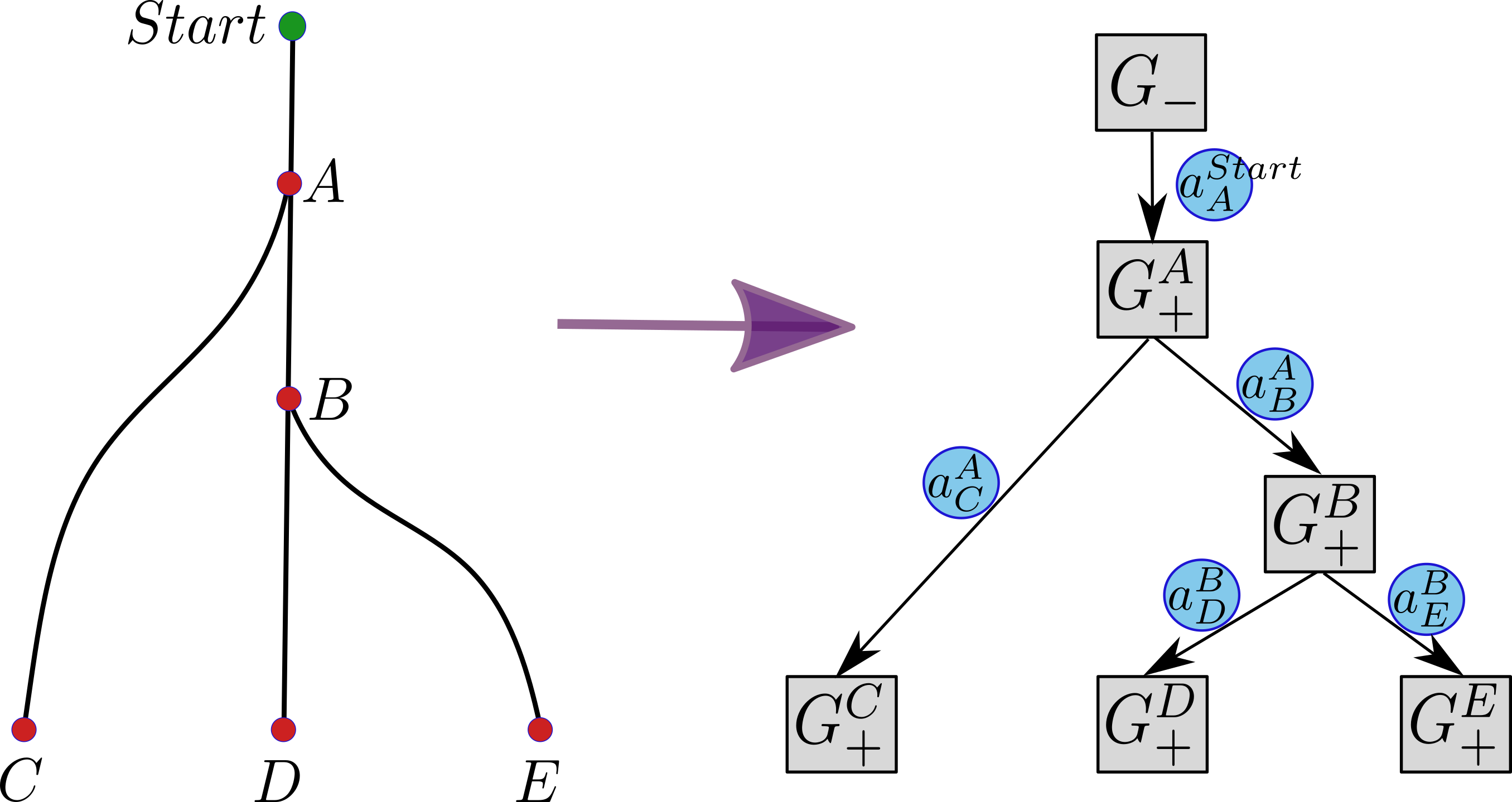
(a)

Figure 4: Different candidate trajectories and their FGP action tree representation. $A$ and $B$ are splitting waypoints; $C$, $D$ and $E$ are final waypoints of 3 trajectory candidates. Each waypoint has associated factor graph vertex within the tree. Each action $a_{y}^{x}$ is augmenting factor graph with factors/variables gathered by passing path $x\rightarrow y$.

The above concept applies also to more general problem settings, with numerous candidate actions with mutual parts in their increments. An excellent example for this is belief space planning for autonomous navigation. Here, the set of trajectory candidates can be naturally represented as tree of possible paths, and the FGP action tree can be constructed in such a way that each of its intermediate vertices will represent a belief at a specific splitting waypoint of the trajectories (see Figure 4). In such a general case, in order to pick up the optimal action we will need to calculate IG for each one of the tree’s edges. This can be done again by applying rAMDL technique but will require us to know the specific covariance entries for each intermediate vertex within FGP tree. An efficient calculation of these entries is presented in Section 4.2.3, while the overall algorithm to evaluate the FGP tree is summarized in Algorithm 2.

1 Inputs: $T$ : FGP tree

2 Outputs: $a^{*}$ : optimal action

3

4begin:

5      

6      for v: vertex of T do

7             Determine the set of variables $Y$ whose covariances are required by rAMDL in order to calculate IG of action between $v$’s parent and $v$ (variables involved in factors that were introduced by augmenting $v$’s parent to acquire $v$)

8       end for

9      

10      Calculate these covariances (see Section 4.1)

11      Calculate IG of tree’s each edge through rAMDL (e.g. through Eq. (51))

12      Calculate IG of each candidate by summarizing IG along candidate’s trajectory

13      Select candidate $a^{*}$ with maximal IG

14 end

15

Algorithm 2 EvaluateFGPTree evaluates information impact of candidates and picks the one with the biggest impact.

Note that although in this paper we create an FGP action tree with a structure similar to the tree of candidate navigation paths, in general, different structures can be used. For example, if candidates share their trajectories’ terminal part, this part can be represented as first action under root $G_{-}$. As long as tree’s root represents the prior belief $b[X_{-}]$ and the tree has a vertex for posterior belief of each candidate action, it represents the same decision problem. An interesting question that arises is how to find the tree’s structure that provides the biggest calculation re-use between the candidates and can be evaluated most efficiently. We will leave this question for future research.

Also note that the proposed method can be also applied to the scenario where a similar candidate trajectory is evaluated at sequential time steps. Such a candidate trajectory, taking the robot to some location, at each time step may have a different starting section due to robot’s movement since the previous time step, but will have the same terminal section that brings the robot to the aforementioned location (see also (Chaves and Eustice, 2016)). Thus, this candidate trajectory will have similar posterior factor graphs each time it is evaluated. This similarity between posterior factor graphs can be naturally represented through our FGP tree and hereof it is just another application for our BSP approach.

4.2.3 Incremental Covariance Update within FGP Action Tree

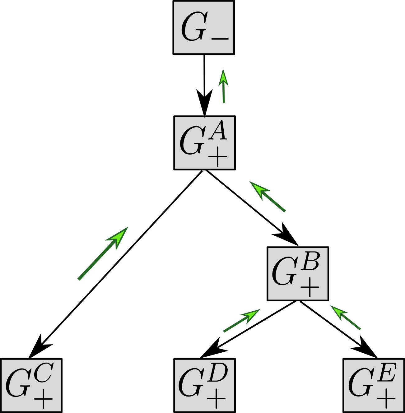
(a)

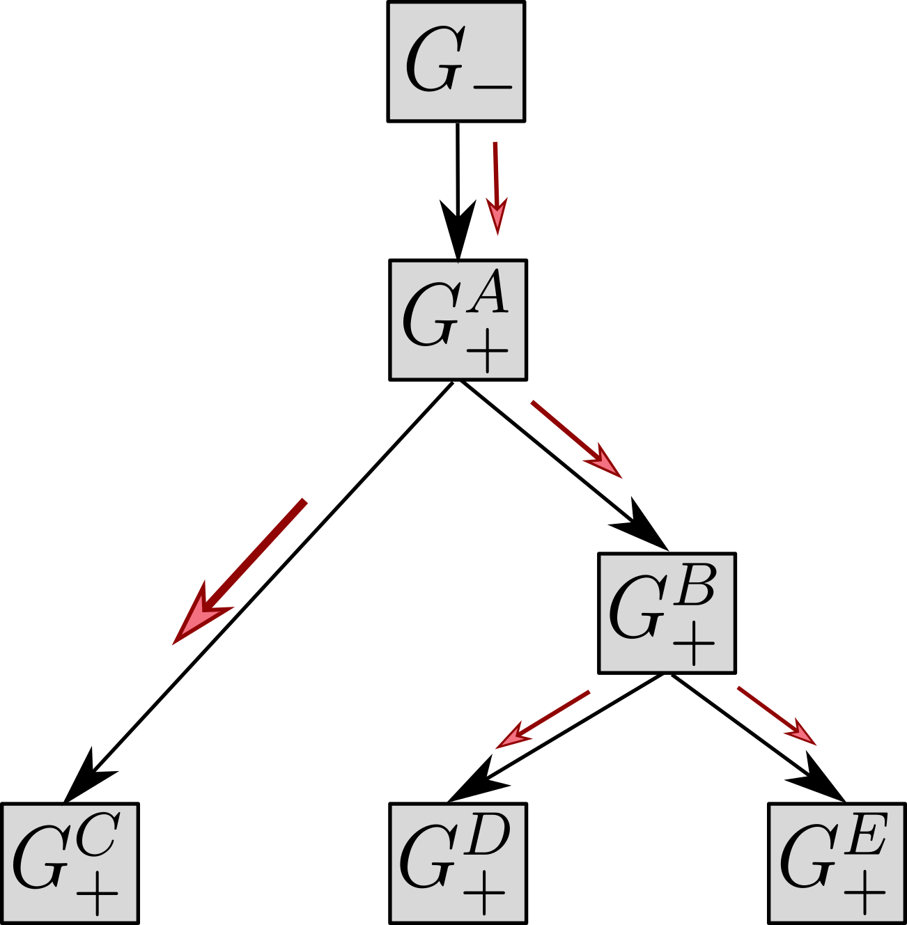
(b)

Figure 5: Incremental covariance update within FGP action tree, illustrated on tree from Figure 4. Each vertex in tree represents specific factor graph and state belief associated with it. Each edge in tree (black arrows) represents action that augments parent’s factor graph in order to obtain the child’s factor graph. The covariance update consists of two stages. First (left drawing): from bottom to top each vertex notifies (green arrows) its parent what are the marginal covariance entries that it needs from parent’s belief. Second (right drawing): from top to bottom each vertex calculates the required marginal covariance entries of its belief and notifies its children (red arrows) to proceed with their covariance calculations. This covariance update process contains one-time calculation depending on state dimension $n$ - computation of required marginal covariance entries at root $G_{-}$. Rest of the calculations is incremental and does not depends on $n$, as described in Section 4.1.

1 Inputs:

2$T$ : FGP tree

3$\{Y_{u}\}$ : set of variables whose covariances from vertex $u$’s belief we are interested in, for each vertex $u$ in $T$

4 Outputs: $\{\Sigma_{u}^{M,Y_{u}}\}$ : the calculated covariances

5

6begin:

7      

8      for u: vertex of T, in bottom-top ordering  do

9             Message $u$’s parent $v$ that we are interested in covariances in $v$’s belief for variables $\{Y_{u},{}^{I}\!X,Y_{ch}\}$, where $Y_{u}$ are variables required by the main algorithm 2, ${}^{I}\!X$ are variables involved in factors that were introduced by augmenting $v$ to acquire $u$, and $Y_{ch}$ are variables that were required by children of $u$

10       end for

11      

12      Define set of variables $Y_{T}\doteq\{Y_{u},Y_{ch}\}$ for each vertex $u$

13      Calculate marginal covariances of $Y_{T}$ at $T$’s root $G_{-}$, $\Sigma_{-}^{M,Y_{T}}$ from prior belief $b[X_{-}]$ (e.g. through Schur Comlement)

14      for u: vertex of T, in top-bottom ordering  do

15             Calculate $\Sigma_{u}^{M,Y_{T}}$ through function $f(\cdot)$ (see Section 4.1.1), by using required covariances $\Sigma_{v}^{M,W}$ from $u$’s parent $v$

16            Retrieve the required $\Sigma_{u}^{M,Y_{u}}$ from calculated $\Sigma_{u}^{M,Y_{T}}$

17       end for

18      

19 end

20

Algorithm 3 CalculateCovariances incrementally calculates specific covariances in the beliefs represented by vetrteces of FGP Action Tree.

In order to reason about different actions inside an FGP action tree, we have to know specific covariance entries for each intermediate vertex in the tree. We can calculate these entries by first propagating the beliefs through Eq. (11) followed by appropriate Schur complement and inverse operations. However, such a procedure will depend on a potentially huge state dimension $n$, which we would like to avoid. Here we propose an alternative method to calculate specific covariance entries at each one of the beliefs inside the tree which is based on our incremental covariance update technique (see Section 4.1) and does not depend on $n$. Moreover, the proposed method can be applied to calculate both specific marginal and conditional covariance entries, where the former are required for the unfocused information objective function (see Eq. (51)) and the latter are required for the focused information objective function (see Eq. (52)).

First of all, let us focus on a specific edge $e_{v\rightarrow u}$ in the FGP tree that represents some action $a$ with increment $I(a)=\{F_{new},X_{new}\}$. In other words, the factor graph represented by $v$ is augmented by $I(a)$ in order to receive the factor graph that is represented by $u$. Also, let us denote state vectors of beliefs of $v$ and of $u$ by $X_{u}$ and $X_{v}$, respectively. Note that $X_{v}\subseteq X_{u}$, and that $X_{u}$ will sometime contain state variables which are not present yet in $X_{v}$ (the variable set $X_{new}$).

Now, consider the set of variables $Y\subseteq X_{u}$ whose marginal covariance $\Sigma_{u}^{M,Y}$ from $u$’s belief we would like to calculate. As was shown in Section 4.1, $\Sigma_{u}^{M,Y}$ can be calculated efficiently and independently of state dimension $n$, given that we have the marginal covariance of the set $W\doteq\{Y_{old},{}^{I}\!X\}$ from $v$’s belief, where ${}^{I}\!X\subseteq X_{v}$ is the set of involved variables in action $a$ and $Y_{old}$ is the intersection between $Y$ and $X_{v}$. It is important to note that, in a general case, the marginal covariance of $Y_{old}$ is modified after applying some action $a$, i.e. $\Sigma_{u}^{M,Y_{old}}\neq\Sigma_{v}^{M,Y_{old}}$. Similarly to Section 4.1 we can separate all possible actions in the FGP tree into different categories depending on their increments, i.e. not-augmented, rectangular and squared. Consequently, for each action type we can use an appropriate covariance update method in order to calculate $\Sigma_{u}^{M,Y}=f(\Sigma_{v}^{M,W})$.

Next, we can use the mentioned above function $\Sigma_{u}^{M,Y}=f(\Sigma_{v}^{M,W})$ to calculate the required specific covariances for each one of the vertices in the tree recursively (see also Figure 5): First, for each vertex $u$ we define by $Y$ the variables of interest whose marginal covariances $\Sigma_{u}^{M,Y}$ at the belief associated with $u$ we would like to calculate. In our case $Y$ are the variables required by rAMDL in order to evaluate impact of actions that are performed on $u$ (see Section 4.2.2). Next, for each leaf vertex $u$ we message its parent $v$ that we require $v$’s marginal covariances for $\{Y,{}^{I}\!X\}$. Then in recursive form from bottom to top each vertex $v$ will message its parent that it requires its parent’s covariances for $\{Y,{}^{I}\!X,Y_{ch}\}$ where $Y_{ch}$ is the set of variables that were required by $v$’s children. Eventually, for each vertex $v$ in the tree we will have a total set of variables $Y_{T}\doteq\{Y,Y_{ch}\}$ whose covariances we need to compute for this specific vertex.

Finally, we start to propagate these covariances in top to bottom order. Using the equations from Section 4.1.1, for each vertex $u$ we can calculate $\Sigma_{u}^{M,Y_{T}}$ using $\Sigma_{v}^{M,W}$ from its parent vertex $v$. Note that when following top to bottom order, when we get to node $u$, its parent’s covariances $\Sigma_{v}^{M,W}$ will be already computed. Also note that the required prior covariance entries of the root $G_{-}$ should be calculated first. This is done only once and its complexity depends on state dimension $n$, similarly to rAMDL technique. But once calculated, the rest of the covariance updates do not depend on $n$.

To summarize, the described algorithm consists of two parts - detecting variables set $Y_{T}$ for each vertex and propagating specific covariances from top to bottom. See Algorithm 3 and a schematic illustration of the incremental covariance update in Figure 5. The runtime complexity of the algorithm mainly depends on its second part, since variable detection does not require any matrix manipulations and can be done fast. The second part handles each edge of the FGP tree only once, thus again allowing us to evaluate mutual increment of actions only once. Run-time to propagate specific covariances along each edge depends on a number of parameters such as dimension of required covariances and size of action’s increment.

In a similar way we can also incrementally propagate specific conditional covariances along the FGP tree. Such covariances may also be required in order to perform informative-theoretic decision making when we want to reduce uncertainty of a subset of old variables $X^{F}\subseteq X_{-}$, see (Kopitkov and Indelman, 2017).

5 Results

We evaluate the proposed approaches for incremental covariance update and BSP in simulation considering the problem of autonomous navigation in unknown environments. The robot has to autonomously visit a set of predefined goals while localizing itself and mapping the environment using its onboard sensors. In our simulation, we currently consider a monocular camera and a range sensor. The code is implemented in Matlab and uses the GTSAM library(Dellaert, 2012; Kaess et al., 2012). All scenarios were executed on a Linux machine with i7 2.40 GHz processor and 32 Gb of memory. All compared approaches were implemented in single thread to provide better visualization of their runtime complexity. Additionally, we provide our implementation of FGP action tree as open-source library in ”http://goo.gl/dmNenc”.

5.1 Covariance Recovery

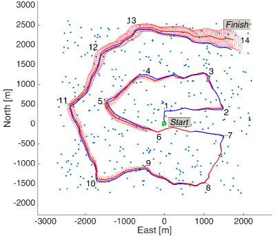
(a)

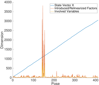
(b)

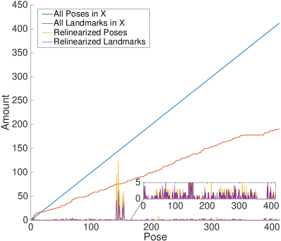
(c)

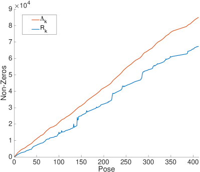
(d)

Figure 6: Robot follows predefined path by navigating through given way-points. (a) Robot trajectory. Blue dots are mapped landmarks, red line with small ellipses is estimated trajectory with pose covariances, blue line is the real trajectory, pluses with numbers beside them are robot’s predefined goals. Green mark is robot’s start position; (b) Dimensions at each timestep of state vector $X$, of overall introduced and relinearized factors and of involved variables in these factors; (c) Number of overall poses/landmarks inside state vector $X$ and number of relinearized poses/landmarks; (d) Number of non-zero entries inside the information matrix $\Lambda_{k}$ and the square-root information matrix $R_{k}$.

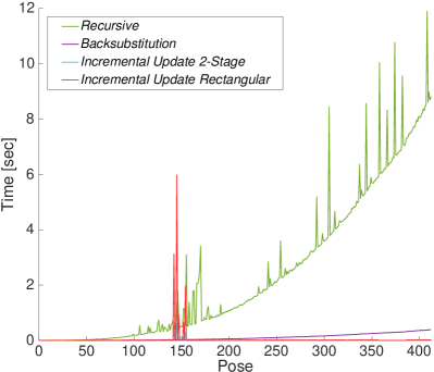
(a)

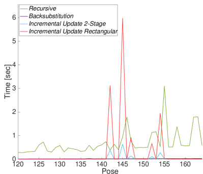
(b)

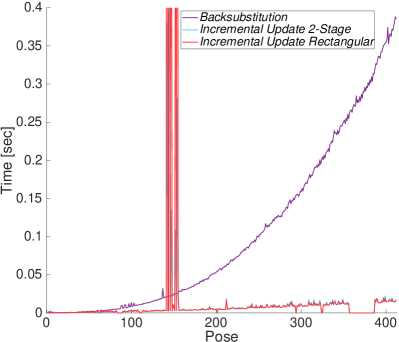
(c)

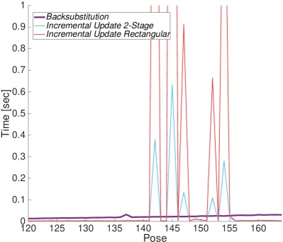
(d)

Figure 7: Robot follows predefined path by navigating through given way-points. (a) Running time of marginal covariance recovery, i.e. evaluating the marginal covariance matrix for each pose and each landmark; (b) Running time from (a) with zoom-in on loop-closure around pose 150; (c) Running time from (a) with zoom-in on three fastest approaches; (d) Running time from (c) with zoom-in on loop-closure around pose 150.

Here we consider the passive setting where at each time step the robot moves toward the next predefined goal (see Figure 6), updates the inference problem with new pose/landmarks and motion/measurement factors, and calculates/updates marginal covariance of each variable inside the state vector.

We apply our incremental covariance update methods (2-stage and Rectangular) as it was described in Section 4.1.4. Their performance is compared with two baseline approaches. First, Recursive, uses a recursive formulation (see Eqs. (6)-(7)) to calculate the covariance matrix $\Sigma_{k}$ ($k$ is index of time step) from a square-root information matrix $R_{k}$. It is done for each $k$ and entire $\Sigma_{k}$ is calculated at each time step from scratch. Note that to calculate the marginal covariance of each state variable (block-diagonal of $\Sigma_{k}$) the Recursive method requires to calculate the entire covariance matrix $\Sigma_{k}$ as was explained in Problem 1 from Section 3.

The second approach, Backsubstitution, calculates $\Sigma_{k}$ through the backsubstitution operation:

$$V\triangleq R_{k}\diagdown I,\quad\Sigma_{k}=V\cdot V^{T}$$ (54)

where $I$ is an identity matrix of appropriate dimensions and ”$\diagdown$” is the Matlab’s backsubstitution operator with $x=A\diagdown B$ being identical to solving linear equations $Ax=B$ for $x$. Such backsubstitution can be done very efficiently since the matrix $R_{k}$ is upper triangular and sparse. Still, similar to Recursive, the Backsubstitution method calculates covariances from scratch for each time step and needs to calculate the entire $\Sigma_{k}$ matrix before fetching its diagonal blocks.

As can be seen in Figure 7, in general both our incremental approaches have very similar runtime, and the both are significantly faster than the baseline alternatives. Towards the end of the scenario, while the fastest alternative (Backsubstitution) needs almost 400 ms to recover marginal covariance for a 3054-dimensional state vector, our incremental method does it in only 20 ms.

The only time our methods are slower than the alternatives is around pose 150, at which point a loop-closure event occurs: the robot reaches a predefined goal 6 (see Figure 6a) and observes old landmarks from the beginning of the scenario. As expected for such a relatively big loop-closure, the number of relinearized state variables and the affected factors is very large (see Figures 6b-6c). Thus, $m$ (overall dimension of new/relinearized factors) and $|{}^{I}\!X|$ (dimension of involved variables) are huge and increase the runtime complexity of our incremental method. However, such results are expected; it is a known fact that incremental techniques become slower in presence of big loop-closures. For example, the incremental optimization algorithm iSAM2 (Kaess et al., 2012), which calculates incrementally the MAP estimate of the state but not its covariance matrix, takes significantly more time during loop-closure events. It is reasonable to expect a similar situation also in the context of incremental covariance recovery. Also note that during a loop-closure event, the Rectangular technique is significantly slower than the 2-stage technique (around 6s vs 0.6s respectively). The reason is that during huge loop-closure, $m$ impacts the entire calculation of the Rectangular method (Lemma 2), while in the 2-stage technique only the second stage is affected (Lemma 1 or Lemma 4). Lemma 2 is more computationally demanding than Lemma 1 or Lemma 4, thus producing such a big runtime difference during a loop closure.

On the other hand, the Backsubstitution method does not depend on $m$ or $|{}^{I}\!X|$; instead its complexity mainly depends on the state dimension $n$ and the sparsity level of a matrix $R_{k}$. The $n$, the overall dimension of all state variables, is not affected by loop-closures. While in general the matrix $R_{k}$ (a factorization of information matrix $\Lambda_{k}$) becomes denser during the loop-closures, an appropriate variable reordering (of the entire matrix) can mitigate this effect. In our simulations we used SYMAMD ordering (symmetric approximate minimum degree permutation, (Amestoy et al., 1996)) to reorder an entire $\Lambda_{k}$ before producing $R_{k}$. As can be seen in Figure 6d (blue line), the resulting sparsity of $R_{k}$ grows smoothly with time, with only a minor increase during the loop-closure event (around pose 150). Thus, we can see no peaks in calculation time plot of Backsubstitution approach around this time (see Figures 7c-7d, purple line). In practice, when implementing our incremental approach on a real robot, to handle this loop-closure shortcoming we can check if a big loop-closure happens ($m$ or $|{}^{I}\!X|$ are bigger than current state dimension $n$) and use Backsubstitution as a fallback.

Comparing Recursive vs Backsubstitution we can see that the former is considerably slower. The first was implemented by us in C++ code, while the second is based on highly optimized Matlab implementation of backsubstitution. Apparently, our current C++ implementation of Recursive method is not properly optimized. We foresee that it can be done in much better way so that both Recursive vs Backsubstitution techniques will have very similar runtime complexity.

We note we did not compare our approach with the one from (Ila et al., 2015) since their method is limited and cannot be applied for every case of inference change, as was described already above. For example, the study (Ila et al., 2015) explicitly states that when any variable was relinearized during the change in the inference problem, the Recursive method is used to recover the marginal covariances. In Figure 6c we can see that this applies to the most of the changes in our scenario since small number of state variables is relinearized at almost any time step. Nonetheless, for cases supported by the technique from (Ila et al., 2015) we expect to see performance very similar to the one of our own approach, since runtime of both methods depends on $m$ and $|{}^{I}\!X|$.

Additionally, the incremental recovery of conditional covariance entries is essential to efficiently solve information-theoretic BSP problem which is considered in Section 5.2; this important scenario is also not supported in (Ila et al., 2015).

5.2 Belief Space Planning

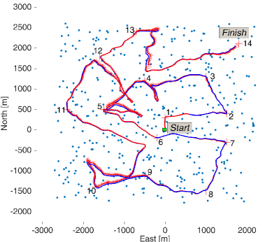
(a)

(b)

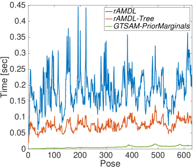
(c)

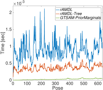
(d)

Figure 8: Focused BSP scenario with focused robot’s last pose. (a) Final robot trajectory. Blue dots are mapped landmarks, red line with small ellipses is estimated trajectory with pose covariances, blue line is the real trajectory, red pluses with numbers beside them are robot’s predefined goals. Green mark is robot’s start position; (b) Number of action candidates at each time; (c) Running time of planning, i.e. evaluating impact of all candidate actions, each representing possible trajectory; (d) Running time from (c) normalized by number of candidates.

(a)

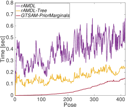
(b)

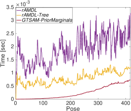
(c)

Figure 9: Focused BSP scenario with focused mapped till now landmarks. (a) Number of action candidates at each time; (b) Running time of planning, i.e. evaluating impact of all candidate actions, each representing possible trajectory; (c) Running time from (b) normalized by number of candidates.

Thus far, we performed simulation of a passive SLAM problem, where robot follows a predefined trajectory. As can be seen in Figure 6a, by the end of the trajectory the covariance of robot position (red ellipse) is considerably big. Such uncertainty in robot localization may fail the navigation task and is undesirable in general. In this section we focus on an active SLAM scenario, where the robot autonomously decides whether to follow the navigation path or to perform a loop-closure and reduce state uncertainty. At each time step, the robot autonomously decides its next action according to a specified objective function that is discussed below.

We compare performance of the proposed BSP approach, that we denote as rAMDL-Tree, with our previous method rAMDL (Kopitkov and Indelman, 2017), which was shown to be superior in run-time complexity to other state-of-the-art information-based BSP methods. Note that both rAMDL and rAMDL-Tree, as well as other relevant state-of-the-art alternatives, make identical decisions, i.e. calculate the same optimal actions. Thus, the only difference is the run-time complexity, reduction of which is the main motivation behind the work presented herein.

In our simulation, at each time step we sample a set of trajectories to the current goal $g$, and also to (clusters of) already mapped landmarks for uncertainty reduction via loop closures (see Figure 8a). The overall number of candidate actions (number of trajectories) is around 200. We consider the objective function

$$J(a)=\alpha_{1}d(x_{k+L},g)+\alpha_{2}c(a)+\alpha_{3}J_{inf}(a),$$ (55)

where $d(x_{k+L},g)$ is the distance between the current goal $g$ and candidate’s last pose $x_{k+L}$ for a given action $a$, $c(a)$ is the control cost, and $J_{inf}(a)$ is an information-theoretic term. As was mentioned before, both first and second terms can be calculated very fast and do not require belief propagation. Thus, in the sequel we will ignore these terms and discuss run time only for the term $J_{inf}(a)$.

In our first simulation, $J_{inf}(a)$ calculates the posterior entropy of robot’s last pose $x_{k+L}$ within the candidate trajectory. We evaluated this term for all action candidates independently through our previous method, rAMDL, and through the proposed-herein approach, rAMDL-Tree, which, using the FGP action tree, accounts for candidate actions’ mutual parts and evaluates them only once. In Figures 8c-8d we can see that rAMDL-Tree is twice faster than rAMDL and succeeds to evaluate more than 200 actions in less than 100ms. Also, we can see that the only algorithmic part that depends on the state dimension $n$, i.e. the one-time calculation of prior covariances at $G_{-}$ during the incremental covariance update termed in the figure as GTSAM-PriorMarginals, takes a small portion of the overall run-time (green lines in Figures 8c-8d); most of the time is consumed by propagation of covariance entries within the FGP action tree and IG calculation for each edge in this tree. Note that the marginal/conditional covariances required by rAMDL-Tree are propagated from the root of FGP action tree to its leafs based on our incremental covariance update technique (see Section 4.1). Specifically, as described in Section 4.2.3, covariance propagation is performed in two phases. In the first one, each tree node in bottom-to-top order determines what covariance entries are required from its belief. In the second phase the required covariances are calculated in top-to-bottom order using incremental covariance update lemmas (see also Figure 5).

Additionally, we have performed a similar simulation considering this time $J_{inf}(a)$ calculating the IG of the landmarks that were mapped till now. The results are shown in Figure 9. Comparing the time-performance between the first and second scenarios we can see that ”focused-landmarks” requires more time; while rAMDL-Tree takes around 50-100ms in the first one, it requires 100-250ms in the second. This is due to the fact that calculation of the focused IG contains a one-time computation that depends on the dimension of focused variables set $X^{F}_{+}$. In ”focused-landmarks” scenario this is the dimension of all landmarks mapped thus far, and it increases with time as more landmarks are observed and introduced into the state vector. Also in this scenario we see a similar trend where rAMDL-Tree performs twice faster than rAMDL (100-250ms vs 200-500ms), while determining the same optimal actions.

6 Conclusions

We developed computationally efficient approaches that address incremental covariance recovery and BSP over high-dimensional state spaces. Our incremental covariance update technique allows to efficiently update specific covariance entries (both marginal and conditional) after any change in the inference problem, including introduction of new state variables, addition of new measurement factors, and relinearization of the entire state vector or only a subset of the state variables. It can be applied whenever an efficient method is required to track covariance entries within the estimation system (e.g. in SLAM for data association or safety), and is also an indispensable part of our BSP approach.

Furthermore, considering the BSP problem our key observation is that in many robotics applications, candidate actions have mutual parts where each part can be evaluated only once, independently of the number of candidate actions that share it. For this purpose, we presented a novel approach to model future posterior beliefs of different candidate actions within a single graphical model which we called factor-graph propagation (FGP) action tree. This tree model allows to evaluate shared parts of different actions only once by representing belief propagation of posterior factor graphs from current factor graph sequentially. The FGP action tree has a consecutive hierarchic form, with intermediate vertices that represent beliefs after applying only part of a candidate action. Further, we use the aforementioned incremental covariance recovery technique to efficiently calculate covariances at intermediate and final state beliefs within the FGP action tree, doing so independently of state dimension $n$. The calculated covariance entries let us reason about probabilistic properties of the beliefs and actions within the FGP action tree. Specifically, this allowed us to efficiently calculate information impact of all candidate actions by re-using calculation from candidates’ mutual parts. Overall, our method involves two passes over the FGP action tree, bottom-to-top query of required covariance entries and top-to-bottom propagation of these covariance entries. We evaluated the proposed approach in simulation considering the problem of autonomous navigation in unknown environments, and showed it reduces run-time twice compared to our previous approach (Kopitkov and Indelman, 2017), rAMDL.

There are several avenues for future research to take the proposed concept of re-using calculations between different candidate actions further. In this work we considered a specific realization of the FGP action tree, using the structure of candidate trajectories in an autonomous navigation scenario. However, given posterior factor graphs for different candidate actions, multiple FGP action trees can be constructed. A key question that will be addressed as part of future research is how to construct an FGP action tree so that most of actions’ similarity would be exploited. Another direction for future research is to make BSP runtime complexity totally independent of state dimension. The process of information evaluation via FGP action tree consists of only a single, one-time, calculation that depends on state dimension $n$, i.e. recovering the prior marginal (or conditional) covariance entries of variables involved in candidate actions. When there are many candidates (above 500 in our simulations), this one-time part is insignificant w.r.t. overall process time and can be ignored. However, for a smaller number of candidate actions this part takes considerable time (about 50% of time in our simulation in Figure 9) and additional research efforts are required in order to reduce its time complexity. Anticipating what state variables would be involved in the near-future candidate actions and incrementally tracking specific covariance entries of these involved variables during the inference process through our incremental covariance recovery method may be an appropriate solution and will be investigated in the future.

7 Appendix

7.1 Proof of Lemma 1 - Not-augmented Case

The variables set $W$ in this case is $\{Y_{old},{}^{I}\!X\}=\{Y,{}^{I}\!X\}$. Define prior marginal covariance matrices: $\Sigma_{-}^{I}\equiv\Sigma_{-}^{M,{}^{I}\!X}$, $\Sigma_{-}^{Y}\equiv\Sigma_{-}^{M,Y}$. Also denote the prior cross covariance between $Y$ and ${}^{I}\!X$ as $\Sigma_{-}^{C}$. Then, $\Sigma_{-}^{M,W}$ will have the following form:

$$\Sigma_{-}^{M,W}=\begin{pmatrix}\Sigma_{-}^{Y}&\Sigma_{-}^{C}\\ (\Sigma_{-}^{C})^{T}&\Sigma_{-}^{I}\\ \end{pmatrix}.$$ (56)

Additionally, let us separate prior (old) state variables $X_{-}$ into involved ${}^{I}\!X$ (in new factors $F_{new}$) and not involved ${}^{\neg I}\!X$ variables. Similarly, let us partition the Jacobian matrix $A$ into:

$$A=\begin{pmatrix}{}^{\neg I}\!A&{}^{I}\!A\\ \end{pmatrix}=\begin{pmatrix}0&{}^{I}\!A\\ \end{pmatrix},$$ (57)

where ${}^{\neg I}\!A$ contains noise-weighted Jacobians w.r.t. $X^{\neg I}$, and ${}^{I}\!A$ w.r.t. ${}^{I}\!X$. From its definition we can conclude that ${}^{\neg I}\!A$ contains only zeros.

Next, using the Woodbury matrix identity and information update equation $\Lambda_{+}=\Lambda_{-}+A^{T}\cdot A$, the posterior covariance matrix is:

$$\Sigma_{+}=(\Lambda_{+})^{-1}=(\Lambda_{-}+A^{T}\cdot A)^{-1}=\Sigma_{-}-\Sigma_{-}\cdot A^{T}\cdot[I_{m}+A\cdot\Sigma_{-}\cdot A^{T}]^{-1}\cdot A\cdot\Sigma_{-}=\Sigma_{-}-\Sigma_{-}\cdot A^{T}\cdot[I_{m}+{}^{I}\!A\cdot\Sigma_{-}^{I}\cdot({}^{I}\!A)^{T}]^{-1}\cdot A\cdot\Sigma_{-}$$ (58)

where $A\cdot\Sigma_{-}\cdot A^{T}={}^{I}\!A\cdot\Sigma_{-}^{I}\cdot({}^{I}\!A)^{T}$ because of $A$’s sparsity structure.

Then $\Sigma_{+}$ can be calculated as:

$$\Sigma_{+}=\Sigma_{-}-\Sigma_{-}\cdot A^{T}\cdot C^{-1}\cdot A\cdot\Sigma_{-}$$ (59)

$$C=I_{m}+{}^{I}\!A\cdot\Sigma_{-}^{I}\cdot({}^{I}\!A)^{T}.$$ (60)

Further, $\Sigma_{+}^{M,Y}$ can be calculated by retrieving from $\Sigma_{+}$ rows and columns that belong to variables $Y$:

$$\Sigma_{+}^{M,Y}=\Sigma_{-}^{M,Y}-\Sigma_{-}^{(Y,:)}\cdot A^{T}\cdot C^{-1}\cdot A\cdot\Sigma_{-}^{(:,Y)}=\Sigma_{-}^{M,Y}-[A\cdot\Sigma_{-}^{(:,Y)}]^{T}\cdot C^{-1}\cdot[A\cdot\Sigma_{-}^{(:,Y)}]=\\ =\Sigma_{-}^{M,Y}-[{}^{I}\!A\cdot(\Sigma_{-}^{C})^{T}]^{T}\cdot C^{-1}\cdot[{}^{I}\!A\cdot(\Sigma_{-}^{C})^{T}]=\Sigma_{-}^{M,Y}-[\Sigma_{-}^{C}\cdot({}^{I}\!A)^{T}]\cdot C^{-1}\cdot[\Sigma_{-}^{C}\cdot({}^{I}\!A)^{T}]^{T}$$ (61)

where using Matlab syntax we have $\Sigma_{-}^{(Y,:)}\doteq\Sigma_{-}(Y,:)$ and $\Sigma_{-}^{(:,Y)}\doteq\Sigma_{-}(:,Y)$. $\blacksquare$

Note that the columns inside information matrices do not have to be ordered in any particular way, and that the provided above proof is correct for any ordering whatsoever.

7.2 Proof of Lemma 2 - Rectangular Case

In this case we can partition variables set $Y$ into two subsets $Y_{old}\doteq X_{-}\cap Y$ and $Y_{new}\doteq X_{new}\cap Y$, or in other words, into old and new state variables. The posterior marginal covariance matrix $\Sigma_{+}^{M,Y}$ will have then the following form:

$$\Sigma_{+}^{M,Y}=\begin{pmatrix}\Sigma_{+}^{M,Y_{old}}&\Sigma_{+}^{(Y_{old},Y_{new})}\\ (\Sigma_{+}^{(Y_{old},Y_{new})})^{T}&\Sigma_{+}^{M,Y_{new}}\\ \end{pmatrix},$$ (62)

and we are looking for an efficient way to calculate matrices $\Sigma_{+}^{M,Y_{old}}$, $\Sigma_{+}^{M,Y_{new}}$ and $\Sigma_{+}^{(Y_{old},Y_{new})}$.

The variables set $W$ in this case is $\{Y_{old},{}^{I}\!X\}$. Define next the prior marginal covariance matrices: $\Sigma_{-}^{I}\equiv\Sigma_{-}^{M,{}^{I}\!X}$, $\Sigma_{-}^{Y_{old}}\equiv\Sigma_{-}^{M,Y_{old}}$. Also denote the prior cross covariance between $Y_{old}$ and ${}^{I}\!X$ as $\Sigma_{-}^{C}$. Then, $\Sigma_{-}^{M,W}$ will have the following form:

$$\Sigma_{-}^{M,W}=\begin{pmatrix}\Sigma_{-}^{Y_{old}}&\Sigma_{-}^{C}\\ (\Sigma_{-}^{C})^{T}&\Sigma_{-}^{I}\\ \end{pmatrix}.$$ (63)

Additionally, let us separate prior (old) state variables $X_{-}$ into involved ${}^{I}\!X$ (in new factors $F_{new}$) and not involved ${}^{\neg I}\!X$. The posterior state vector is then $X_{+}=\{{}^{I}\!X,{}^{\neg I}\!X,X_{new}\}$. Similarly, let us partition the Jacobian matrix $A$ into:

$$A=\begin{pmatrix}A_{old}&A_{new}\\ \end{pmatrix},\quad A_{old}=\begin{pmatrix}{}^{\neg I}\!A&{}^{I}\!A\\ \end{pmatrix}=\begin{pmatrix}0&{}^{I}\!A\\ \end{pmatrix},$$ (64)

where $A_{old}$ contains noise-weighted Jacobians w.r.t. old variables $X_{-}$, $A_{new}$ w.r.t. new variables $X_{new}$, ${}^{\neg I}\!A$ w.r.t. ${}^{\neg I}\!X$, and ${}^{I}\!A$ w.r.t. ${}^{I}\!X$. From its definition we can conclude that ${}^{\neg I}\!A$ contains only zeros.

Following the information update equation $\Lambda_{+}=\Lambda_{+}^{Aug}+A^{T}\cdot A$ (see also Figure 3), the posterior information matrix can be partitioned using separation $X_{+}=\{X_{-},X_{new}\}$ as:

$$\Lambda_{-}=\begin{pmatrix}\Lambda_{-}+A_{old}^{T}\cdot A_{old}&A_{old}^{T}\cdot A_{new}\\ A_{new}^{T}\cdot A_{old}&A_{new}^{T}\cdot A_{new}\\ \end{pmatrix}.$$ (65)

Now, let us partition the posterior covariance matrix $\Sigma_{+}$ in a similar way:

$$\Sigma_{+}=\begin{pmatrix}\Sigma_{+}^{old}&\Sigma_{+}^{cross}\\ (\Sigma_{+}^{cross})^{T}&\Sigma_{+}^{new}\\ \end{pmatrix}.$$ (66)

Giving the setup till now, we will derive each of the matrices $\Sigma_{+}^{M,Y_{old}}$, $\Sigma_{+}^{M,Y_{new}}$ and $\Sigma_{+}^{(Y_{old},Y_{new})}$ from Eq. (62) using parts from $\Sigma_{-}^{M,W}$ defined in Eq. (63).

$\bm{\Sigma_{+}^{M,Y_{new}}}$:

By using block-wise matrix inversion (which is based on the notion of Schur Complements), $\Sigma_{+}^{new}$ is equal to:

$$\Sigma_{+}^{new}=(A_{new}^{T}\cdot A_{new}-A_{new}^{T}\cdot A_{old}\cdot(\Lambda_{-}+A_{old}^{T}\cdot A_{old})^{-1}\cdot A_{old}^{T}\cdot A_{new})^{-1}=(A_{new}^{T}\cdot(I_{m}-A_{old}\cdot(\Lambda_{-}+A_{old}^{T}\cdot A_{old})^{-1}\cdot A_{old}^{T})\cdot A_{new})^{-1}$$ (67)

Now, let’s define matrix $C$ as following:

$$C\triangleq I_{m}+A_{old}\cdot\Sigma_{-}\cdot A_{old}^{T}=I_{m}+{}^{I}\!A\cdot\Sigma_{-}^{I}\cdot({}^{I}\!A)^{T}.$$ (68)

Through Woodbury matrix identity it can be easily shown that $C$’s inverse is:

$$C^{-1}=I-A_{old}\cdot(\Lambda_{-}+A_{old}^{T}\cdot A_{old})^{-1}\cdot A_{old}^{T}.$$ (69)

Therefore, $\Sigma_{+}^{new}$ is equal to:

$$\Sigma_{+}^{new}=(A_{new}^{T}\cdot C^{-1}\cdot A_{new})^{-1},$$ (70)

and $\Sigma_{+}^{M,Y_{new}}$ can be calculated in the following way (note that such calculation’s complexity is independent of state dimension):

$$\Sigma_{+}^{M,Y_{new}}=P^{(Y_{new},:)},\quad P\triangleq[(A_{new}^{T}\cdot C^{-1}\cdot A_{new})^{-1}]^{(:,Y_{new})},$$ (71)

where in brackets we are using Matlab syntax to index relevant rows/columns. Note that $[(A_{new}^{T}\cdot C^{-1}\cdot A_{new})^{-1}]^{(:,Y_{new})}$ can be calculated without calculation of full $(A_{new}^{T}\cdot C^{-1}\cdot A_{new})^{-1}$, by using backslash operator in Matlab:

$$P=[A_{new}^{T}\cdot C^{-1}\cdot A_{new}]\backslash I^{(:,Y_{new})},$$ (72)

where $I^{(:,Y_{new})}$ are particular columns of identity matrix.

$\bm{\Sigma_{+}^{M,Y_{old}}}$:

Using the block-wise matrix inversion again we know that $\Sigma_{+}^{old}$ from Eq. (66) is equal to:

$$\Sigma_{+}^{old}=(\Lambda_{-}+A_{old}^{T}\cdot A_{old}-A_{old}^{T}\cdot A_{new}\cdot(A_{new}^{T}\cdot A_{new})^{-1}\cdot A_{new}^{T}\cdot A_{old})^{-1}=\\ =(\Lambda_{-}+A_{old}^{T}\cdot(I_{m}-A_{new}\cdot(A_{new}^{T}\cdot A_{new})^{-1}\cdot A_{new}^{T})\cdot A_{old})^{-1}=(\Lambda_{k}+A_{old}^{T}\cdot K\cdot A_{old})^{-1}$$ (73)

with

$$K\triangleq I_{m}-A_{new}\cdot(A_{new}^{T}\cdot A_{new})^{-1}\cdot A_{new}^{T}=I_{m}-A_{new}\cdot F\cdot A_{new}^{T},\quad F\triangleq(A_{new}^{T}\cdot A_{new})^{-1},$$ (74)

where $K$ is a singular, symmetric, idempotent projection matrix, with properties $K=K^{2}$ and $K=K^{T}$.

Further, $\Sigma_{+}^{old}$ can be now rewritten as:

$$\Sigma_{+}^{old}=(\Lambda_{-}+A_{old}^{T}\cdot K^{T}\cdot K\cdot A_{old})^{-1}=\Lambda_{-}^{-1}-\Lambda_{-}^{-1}\cdot A_{old}^{T}\cdot K^{T}\cdot(I_{m}+K\cdot A_{old}\cdot\Lambda_{-}^{-1}\cdot A_{old}^{T}\cdot K^{T})^{-1}\cdot K\cdot A_{old}\cdot\cdot\Lambda_{-}^{-1}=\\ =\Sigma_{-}-\Sigma_{-}\cdot A_{old}^{T}\cdot K^{T}\cdot(I_{m}+K\cdot A_{old}\cdot\Sigma_{-}\cdot A_{old}^{T}\cdot K^{T})^{-1}\cdot K\cdot A_{old}\cdot\cdot\Sigma_{-}=\Sigma_{-}-\Sigma_{-}\cdot A_{old}^{T}\cdot K^{T}\cdot G^{-1}\cdot K\cdot A_{old}\cdot\Sigma_{-}$$ (75)

with

$$G\triangleq I_{m}+K\cdot A_{old}\cdot\Sigma_{-}\cdot A_{old}^{T}\cdot K^{T}=I_{m}+K\cdot{}^{I}\!A\cdot\Sigma_{-}^{I}\cdot({}^{I}\!A)^{T}\cdot K^{T}=I_{m}+K_{1}\cdot\Sigma_{-}^{I}\cdot K_{1}^{T}$$ (76)

$$K_{1}\triangleq K\cdot{}^{I}\!A,$$ (77)

where $K_{1}$ are non-zero columns from $A_{old}$ projected outside of vector space that is spanned by columns in $A_{new}$. In other words, $K_{1}$ contains information from $A_{old}$ that is not contained within $A_{new}$.

Then $\Sigma_{+}^{M,Y_{old}}$ can be calculated by retrieving from $\Sigma_{+}^{old}$ rows and columns that belong to variables $Y_{old}$:

$$\Sigma_{+}^{M,Y_{old}}=\Sigma_{-}^{M,Y_{old}}-\Sigma_{-}^{(Y_{old},:)}\cdot A_{old}^{T}\cdot K^{T}\cdot G^{-1}\cdot K\cdot A_{old}\cdot\Sigma_{-}^{(:,Y_{old})}=\Sigma_{-}^{M,Y_{old}}-[K\cdot A_{old}\cdot\Sigma_{-}^{(:,Y_{old})}]^{T}\cdot G^{-1}\cdot[K\cdot A_{old}\cdot\Sigma_{-}^{(:,Y_{old})}]=\\ =\Sigma_{-}^{M,Y_{old}}-[K\cdot{}^{I}\!A\cdot\Sigma_{-}^{(X^{I},Y_{old})}]^{T}\cdot G^{-1}\cdot[K\cdot{}^{I}\!A\cdot\Sigma_{-}^{(X^{I},Y_{old})}]=\Sigma_{-}^{M,Y_{old}}-[K_{1}\cdot(\Sigma_{-}^{C})^{T}]^{T}\cdot G^{-1}\cdot[K_{1}\cdot(\Sigma_{-}^{C})^{T}]=\Sigma_{-}^{M,Y_{old}}-B\cdot G^{-1}\cdot B^{T}$$ (78)

where

$$B\triangleq\Sigma_{-}^{C}\cdot K_{1}^{T}=\Sigma_{-}^{C}\cdot({}^{I}\!A)^{T}\cdot K.$$ (79)

$\bm{\Sigma_{+}^{(Y_{old},Y_{new})}}$ - Method 1:

Using the block-wise matrix inversion again we know that $\Sigma_{+}^{cross}$ from Eq. (66) is equal to:

$$\Sigma_{+}^{cross}=-(\Lambda_{-}+A_{old}^{T}\cdot A_{old})^{-1}\cdot A_{old}^{T}\cdot A_{new}\cdot(A_{new}^{T}\cdot C^{-1}\cdot A_{new})^{-1}=\\ =-(\Sigma_{-}-\Sigma_{-}\cdot A_{old}^{T}\cdot C^{-1}\cdot A_{old}\cdot\Sigma_{-})\cdot A_{old}^{T}\cdot A_{new}\cdot(A_{new}^{T}\cdot C^{-1}\cdot A_{new})^{-1}=\\ =-\Sigma_{-}\cdot A_{old}^{T}\cdot A_{new}\cdot(A_{new}^{T}\cdot C^{-1}\cdot A_{new})^{-1}+\Sigma_{-}\cdot A_{old}^{T}\cdot C^{-1}\cdot A_{old}\cdot\Sigma_{-}\cdot A_{old}^{T}\cdot A_{new}\cdot(A_{new}^{T}\cdot C^{-1}\cdot A_{new})^{-1}=\\ =\Sigma_{-}\cdot A_{old}^{T}\cdot[-I_{m}+C^{-1}\cdot A_{old}\cdot\Sigma_{-}\cdot A_{old}^{T}]\cdot A_{new}\cdot(A_{new}^{T}\cdot C^{-1}\cdot A_{new})^{-1}=\\ =\Sigma_{-}\cdot A_{old}^{T}\cdot[C^{-1}\cdot{}^{I}\!A\cdot\Sigma_{-}^{I}\cdot({}^{I}\!A)^{T}-I_{m}]\cdot A_{new}\cdot(A_{new}^{T}\cdot C^{-1}\cdot A_{new})^{-1},$$ (80)

where matrix $C$ is defined in Eq. (68)

Then $\Sigma_{+}^{(Y_{old},Y_{new})}$ can be calculated by retrieving from $\Sigma_{+}^{cross}$ the entries that correspond to $Y_{old}$ rows and $Y_{new}$ columns:

$$\Sigma_{+}^{(Y_{old},Y_{new})}=\Sigma_{-}^{(Y_{old},:)}\cdot A_{old}^{T}\cdot[C^{-1}\cdot{}^{I}\!A\cdot\Sigma_{-}^{I}\cdot({}^{I}\!A)^{T}-I_{m}]\cdot A_{new}\cdot[(A_{new}^{T}\cdot C^{-1}\cdot A_{new})^{-1}]^{(:,Y_{new})}=\Sigma_{-}^{C}\cdot({}^{I}\!A)^{T}\cdot[C^{-1}\cdot{}^{I}\!A\cdot\Sigma_{-}^{I}\cdot({}^{I}\!A)^{T}-I_{m}]\cdot A_{new}\cdot P$$ (81)

where matrix $P$ is defined in Eq. (71).

$\bm{\Sigma_{+}^{(Y_{old},Y_{new})}}$ - Method 2:

Using another form of block-wise matrix inversion, $\Sigma_{+}^{cross}$ from Eq. (66) is equal to:

$$\Sigma_{+}^{cross}=-[\Sigma_{-}-\Sigma_{-}\cdot A_{old}^{T}\cdot K^{T}\cdot G^{-1}\cdot K\cdot A_{old}\cdot\cdot\Sigma_{-}]\cdot A_{old}^{T}\cdot A_{new}\cdot(A_{new}^{T}\cdot A_{new})^{-1}=\\ =[\Sigma_{-}\cdot A_{old}^{T}\cdot K^{T}\cdot G^{-1}\cdot K\cdot A_{old}\cdot\cdot\Sigma_{-}\cdot A_{old}^{T}-\Sigma_{-}\cdot A_{old}^{T}]\cdot A_{new}\cdot(A_{new}^{T}\cdot A_{new})^{-1}=\\ =[\Sigma_{-}\cdot A_{old}^{T}\cdot K^{T}\cdot G^{-1}\cdot K\cdot A_{old}\cdot\cdot\Sigma_{-}\cdot A_{old}^{T}-\Sigma_{-}\cdot A_{old}^{T}]\cdot A_{new}\cdot F=\\ =[\Sigma_{-}\cdot A_{old}^{T}\cdot K^{T}\cdot G^{-1}\cdot K\cdot{}^{I}\!A\cdot\Sigma_{-}^{I}\cdot({}^{I}\!A)^{T}-\Sigma_{-}\cdot A_{old}^{T}]\cdot A_{new}\cdot F$$ (82)

where matrix $F$ is defined in Eq. (74).

Then $\Sigma_{+}^{(Y_{old},Y_{new})}$ can be calculated by retrieving from $\Sigma_{+}^{cross}$ the entries that correspond to $Y_{old}$ rows and $Y_{new}$ columns:

$$\Sigma_{+}^{(Y_{old},Y_{new})}=[\Sigma_{-}^{(Y_{old},:)}\cdot A_{old}^{T}\cdot K^{T}\cdot G^{-1}\cdot K\cdot{}^{I}\!A\cdot\Sigma_{-}^{I}\cdot({}^{I}\!A)^{T}-\Sigma_{-}^{(Y_{old},:)}\cdot A_{old}^{T}]\cdot A_{new}\cdot F^{(:,Y_{new})}=\\ =[\Sigma_{-}^{C}\cdot({}^{I}\!A)^{T}\cdot K^{T}\cdot G^{-1}\cdot K\cdot{}^{I}\!A\cdot\Sigma_{-}^{I}\cdot({}^{I}\!A)^{T}-\Sigma_{-}^{C}\cdot({}^{I}\!A)^{T}]\cdot A_{new}\cdot F^{(:,Y_{new})}=\\ =\Sigma_{-}^{C}\cdot[({}^{I}\!A)^{T}\cdot K^{T}\cdot G^{-1}\cdot K\cdot{}^{I}\!A\cdot\Sigma_{-}^{I}-I_{k}]\cdot({}^{I}\!A)^{T}\cdot A_{new}\cdot F^{(:,Y_{new})}=\\ =\Sigma_{-}^{C}\cdot[K_{1}^{T}\cdot G^{-1}\cdot K_{1}\cdot\Sigma_{-}^{I}-I_{k}]\cdot({}^{I}\!A)^{T}\cdot A_{new}\cdot F^{(:,Y_{new})}$$ (83)

where matrix $K_{1}$ is defined in Eq. (77) and identity matrix $I_{k}$ has dimension $|{}^{I}\!X|$. $\blacksquare$

Note that the columns inside information matrices do not have to be ordered in any particular way, and that the provided above proof is correct for any ordering whatsoever.

7.3 Proof of Lemma 3 - Squared Case

The squared case is a special instance of the rectangular case, and thus we will use here the same setup as for the rectangular case. In other words, we will use the partitioning that was defined in Eq. (62), (63) and (64).

In squared case we have that $m=|X_{new}|$ from which we can conclude that matrix $A_{new}$ from Eq. (64) is a squared matrix. Then, matrix $K$ from Eq. (24) is equal to zero matrix:

$$K=I_{m}-A_{new}\cdot(A_{new}^{T}\cdot A_{new})^{-1}\cdot A_{new}^{T}=I_{m}-A_{new}\cdot A_{new}^{-1}\cdot(A_{new}^{T})^{-1}\cdot A_{new}^{T}=0.$$ (84)

Further, matrices $K_{1}$ and $B$ from Eq. (25) and Eq. (26) contain only zeros, and $\Sigma_{+}^{M,Y_{old}}$ is equal to:

$$\Sigma_{+}^{M,Y_{old}}=\Sigma_{-}^{M,Y_{old}}-B\cdot G^{-1}\cdot B^{T}=\Sigma_{-}^{M,Y_{old}}.$$ (85)

Next, $\Sigma_{+}^{new}$ from Eq. (70) can be calculated as:

$$\Sigma_{+}^{new}=(A_{new}^{T}\cdot C^{-1}\cdot A_{new})^{-1}=A_{new}^{-1}\cdot C\cdot(A_{new}^{T})^{-1}=A_{new}^{-1}\cdot C\cdot(A_{new}^{-1})^{T},$$ (86)

and $\Sigma_{+}^{M,Y_{new}}$ is equal to:

$$\Sigma_{+}^{M,Y_{new}}=[A_{new}^{-1}]^{(Y_{new},:)}\cdot C\cdot[(A_{new}^{-1})^{T}]^{(:,Y_{new})}=[A_{new}^{-1}]^{(Y_{new},:)}\cdot C\cdot([A_{new}^{-1}]^{(Y_{new},:)})^{T}=A_{iv}\cdot C\cdot A_{iv}^{T},$$ (87)

where

$$A_{iv}\triangleq[A_{new}^{-1}]^{(Y_{new},:)},$$ (88)

and can be efficiently calculated through Matlab backslash operator:

$$A_{iv}=A_{new}\backslash I^{(:,Y_{new})}.$$ (89)

Next, we can reduce Eq. (29) to:

$$\Sigma_{+}^{(Y_{old},Y_{new})}=\Sigma_{-}^{C}\cdot[K_{1}^{T}\cdot G^{-1}\cdot K_{1}\cdot\Sigma_{-}^{I}-I_{k}]\cdot({}^{I}\!A)^{T}\cdot A_{new}\cdot F^{(:,Y_{new})}=\\ =-\Sigma_{-}^{C}\cdot({}^{I}\!A)^{T}\cdot A_{new}\cdot F^{(:,Y_{new})}=-[\Sigma_{-}^{C}\cdot({}^{I}\!A)^{T}\cdot A_{new}\cdot F]^{(:,Y_{new})}=\\ =-[\Sigma_{-}^{C}\cdot({}^{I}\!A)^{T}\cdot A_{new}\cdot A_{new}^{-1}\cdot(A_{new}^{T})^{-1}]^{(:,Y_{new})}=-[\Sigma_{-}^{C}\cdot({}^{I}\!A)^{T}\cdot(A_{new}^{T})^{-1}]^{(:,Y_{new})}=\\ =-\Sigma_{-}^{C}\cdot({}^{I}\!A)^{T}\cdot[(A_{new}^{T})^{-1}]^{(:,Y_{new})}=-\Sigma_{-}^{C}\cdot({}^{I}\!A)^{T}\cdot([A_{new}^{-1}]^{(Y_{new},:)})^{T}=-\Sigma_{-}^{C}\cdot({}^{I}\!A)^{T}\cdot(A_{iv})^{T}$$ (90)

$\blacksquare$

Note that the columns inside information matrices do not have to be ordered in any particular way, and that the provided above proof is correct for any ordering whatsoever.

7.4 Proof of Lemma 4 - Relinearization Case

As we saw in Eq. (38), the information update here has the following form:

$$\Lambda_{+}=\Lambda_{-}+B^{T}\cdot B,\quad B\triangleq\begin{pmatrix}iA_{-}\\ A_{+}\end{pmatrix}.$$ (91)

First, denote by ${}^{I}\!A_{-}$ the non-zero columns of $A_{-}$’s and by ${}^{I}\!A_{+}$ the non-zero columns of $A_{+}$ (note that indices of such columns are the same in both $A_{-}$ and $A_{+}$). Next, apply Lemma 1 as following:

$$\Sigma_{+}^{M,Y}=\Sigma_{-}^{Y}-V\cdot C^{-1}\cdot V^{T},\quad V\triangleq\Sigma_{-}^{C}\cdot({}^{I}\!B)^{T},\quad C\triangleq I_{m}+{}^{I}\!B\cdot\Sigma_{-}^{I}\cdot({}^{I}\!B)^{T},\quad{}^{I}\!B\triangleq\begin{pmatrix}i\cdot{}^{I}\!A_{-}\\ {}^{I}\!A_{+}\end{pmatrix},$$ (92)

where $\Sigma_{-}^{I}\equiv\Sigma_{-}^{M,{}^{I}\!X}$ is the prior marginal covariance of variables ${}^{I}\!X$ involved in the relinearized factors $F_{R}$; $\Sigma_{-}^{Y}\equiv\Sigma_{-}^{M,Y}$ is the prior marginal covariance of variables $Y$; $\Sigma_{-}^{C}$ is the cross-covariance between $Y$ and $X^{I}$.

Next we can see that:

$$C=I_{m}+\begin{pmatrix}i\cdot{}^{I}\!A_{-}\\ {}^{I}\!A_{+}\end{pmatrix}\cdot\Sigma_{-}^{I}\cdot\begin{pmatrix}i\cdot({}^{I}\!A_{-})^{T}&({}^{I}\!A_{+})^{T}\end{pmatrix}=\begin{pmatrix}I-{}^{I}\!A_{-}\cdot\Sigma_{-}^{I}\cdot({}^{I}\!A_{-})^{T}&i\cdot{}^{I}\!A_{-}\cdot\Sigma_{-}^{I}\cdot({}^{I}\!A_{+})^{T}\\ i\cdot{}^{I}\!A_{+}\cdot\Sigma_{-}^{I}\cdot({}^{I}\!A_{-})^{T}&I+{}^{I}\!A_{+}\cdot\Sigma_{-}^{I}\cdot({}^{I}\!A_{+})^{T}\end{pmatrix}\triangleq\begin{pmatrix}C_{11}&i\cdot C_{12}\\ i\cdot C_{12}^{T}&C_{22}\\ \end{pmatrix},$$ (93)

where $I$ is the identity matrix of an appropriate dimension. Note that while $C_{11}$ sometimes can be not positive definite (PD) matrix, $C_{22}$ is always PD and therefore is invertible.

Next, we will use a block-wise inversion in order to calculate $C^{-1}$:

$$C^{-1}\triangleq\begin{pmatrix}C_{11}^{inv}&C_{12}^{inv}\\ (C_{12}^{inv})^{T}&C_{22}^{inv}\\ \end{pmatrix},$$ (94)

$$C_{11}^{inv}\triangleq(C_{11}+C_{12}\cdot C_{22}^{-1}\cdot C_{12}^{T})^{-1},$$ (95)

$$C_{12}^{inv}\triangleq-i\cdot C_{11}^{inv}\cdot C_{12}\cdot C_{22}^{-1},$$ (96)

$$C_{22}^{inv}\triangleq C_{22}^{-1}-C_{22}^{-1}\cdot C_{12}^{T}\cdot C_{11}^{inv}\cdot C_{12}\cdot C_{22}^{-1}.$$ (97)

Using the above notations we can see that:

$$({}^{I}\!B)^{T}\cdot C^{-1}\cdot{}^{I}\!B=\begin{pmatrix}i\cdot({}^{I}\!A_{-})^{T}&({}^{I}\!A_{+})^{T}\end{pmatrix}\cdot\begin{pmatrix}C_{11}^{inv}&C_{12}^{inv}\\ (C_{12}^{inv})^{T}&C_{22}^{inv}\\ \end{pmatrix}\cdot\begin{pmatrix}i\cdot{}^{I}\!A_{-}\\ {}^{I}\!A_{+}\end{pmatrix}=\\ =({}^{I}\!A_{+})^{T}\cdot C_{22}^{-1}\cdot{}^{I}\!A_{+}-({}^{I}\!A_{-})^{T}\cdot C_{11}^{inv}\cdot{}^{I}\!A_{-}+({}^{I}\!A_{-})^{T}\cdot C_{11}^{inv}\cdot C_{12}\cdot C_{22}^{-1}\cdot{}^{I}\!A_{+}+\\ +({}^{I}\!A_{+})^{T}\cdot C_{22}^{-1}\cdot C_{12}^{T}\cdot C_{11}^{inv}\cdot{}^{I}\!A_{-}-({}^{I}\!A_{+})^{T}\cdot C_{22}^{-1}\cdot C_{12}^{T}\cdot C_{11}^{inv}\cdot C_{12}\cdot C_{22}^{-1}\cdot{}^{I}\!A_{+}=\\ =({}^{I}\!A_{+})^{T}\cdot C_{22}^{-1}\cdot{}^{I}\!A_{+}-\Big{[}({}^{I}\!A_{-})^{T}-({}^{I}\!A_{+})^{T}\cdot C_{22}^{-1}\cdot C_{12}^{T}\Big{]}\cdot C_{11}^{inv}\cdot\Big{[}({}^{I}\!A_{-})^{T}-({}^{I}\!A_{+})^{T}\cdot C_{22}^{-1}\cdot C_{12}^{T}\Big{]}^{T}=\\ =({}^{I}\!A_{+})^{T}\cdot C_{22}^{-1}\cdot{}^{I}\!A_{+}-\Big{[}({}^{I}\!A_{-})^{T}-({}^{I}\!A_{+})^{T}\cdot C_{22}^{-1}\cdot C_{12}^{T}\Big{]}\cdot\Big{[}C_{11}+C_{12}\cdot C_{22}^{-1}\cdot C_{12}^{T}\Big{]}^{-1}\cdot\Big{[}({}^{I}\!A_{-})^{T}-({}^{I}\!A_{+})^{T}\cdot C_{22}^{-1}\cdot C_{12}^{T}\Big{]}^{T}=\\ =({}^{I}\!A_{+})^{T}\cdot\Big{[}I+{}^{I}\!A_{+}\cdot\Sigma_{-}^{I}\cdot({}^{I}\!A_{+})^{T}\Big{]}^{-1}\cdot{}^{I}\!A_{+}-\\ -\Bigg{[}({}^{I}\!A_{-})^{T}-({}^{I}\!A_{+})^{T}\cdot\Big{[}I+{}^{I}\!A_{+}\cdot\Sigma_{-}^{I}\cdot({}^{I}\!A_{+})^{T}\Big{]}^{-1}\cdot{}^{I}\!A_{+}\cdot\Sigma_{-}^{I}\cdot({}^{I}\!A_{-})^{T}\Bigg{]}\cdot J^{-1}\cdot\Bigg{[}({}^{I}\!A_{-})^{T}-({}^{I}\!A_{+})^{T}\cdot\Big{[}I+{}^{I}\!A_{+}\cdot\Sigma_{-}^{I}\cdot({}^{I}\!A_{+})^{T}\Big{]}^{-1}\cdot{}^{I}\!A_{+}\cdot\Sigma_{-}^{I}\cdot({}^{I}\!A_{-})^{T}\Bigg{]}^{T},$$ (98)

$$J\triangleq C_{11}+C_{12}\cdot C_{22}^{-1}\cdot C_{12}^{T}=I-{}^{I}\!A_{-}\cdot\Sigma_{-}^{I}\cdot({}^{I}\!A_{-})^{T}+{}^{I}\!A_{-}\cdot\Sigma_{-}^{I}\cdot({}^{I}\!A_{+})^{T}\cdot\Big{[}I+{}^{I}\!A_{+}\cdot\Sigma_{-}^{I}\cdot({}^{I}\!A_{+})^{T}\Big{]}^{-1}\cdot{}^{I}\!A_{+}\cdot\Sigma_{-}^{I}\cdot({}^{I}\!A_{-})^{T}.$$ (99)

Next, introduce new notations:

$$M_{2}\triangleq({}^{I}\!A_{+})^{T}\diagup chol\Big{[}I+{}^{I}\!A_{+}\cdot\Sigma_{-}^{I}\cdot({}^{I}\!A_{+})^{T}\Big{]},$$ (100)

$$G\triangleq M_{2}^{T}\cdot\Sigma_{-}^{I}\cdot({}^{I}\!A_{-})^{T},$$ (101)

where $chol(\cdot)$ represents cholesky decomposition which returns an upper triangular matrix; ”$\diagup$” is the backslash operator from Matlab syntax ($A\diagup B=A\cdot B^{-1}$).

It can be clearly seen that:

$$M_{2}\cdot M_{2}^{T}=({}^{I}\!A_{+})^{T}\cdot\Big{[}I+{}^{I}\!A_{+}\cdot\Sigma_{-}^{I}\cdot({}^{I}\!A_{+})^{T}\Big{]}^{-1}\cdot{}^{I}\!A_{+},$$ (102)

$$G^{T}\cdot G={}^{I}\!A_{-}\cdot\Sigma_{-}^{I}\cdot({}^{I}\!A_{+})^{T}\cdot\Big{[}I+{}^{I}\!A_{+}\cdot\Sigma_{-}^{I}\cdot({}^{I}\!A_{+})^{T}\Big{]}^{-1}\cdot{}^{I}\!A_{+}\cdot\Sigma_{-}^{I}\cdot({}^{I}\!A_{-})^{T},$$ (103)

$$M_{2}\cdot G=({}^{I}\!A_{+})^{T}\cdot\Big{[}I+{}^{I}\!A_{+}\cdot\Sigma_{-}^{I}\cdot({}^{I}\!A_{+})^{T}\Big{]}^{-1}\cdot{}^{I}\!A_{+}\cdot\Sigma_{-}^{I}\cdot({}^{I}\!A_{-})^{T}.$$ (104)

Using matrices $M_{2}$ and $G$, we can rewrite an expression for $({}^{I}\!B)^{T}\cdot C^{-1}\cdot{}^{I}\!B$ as:

$$({}^{I}\!B)^{T}\cdot C^{-1}\cdot{}^{I}\!B=M_{2}\cdot M_{2}^{T}-\Big{[}({}^{I}\!A_{-})^{T}-M_{2}\cdot G\Big{]}\cdot J^{-1}\cdot\Big{[}({}^{I}\!A_{-})^{T}-M_{2}\cdot G\Big{]}^{T},$$ (105)

$$J=I-{}^{I}\!A_{-}\cdot\Sigma_{-}^{I}\cdot({}^{I}\!A_{-})^{T}+G^{T}\cdot G.$$ (106)

Next, let us define another matrix:

$$M_{1}\triangleq\Big{[}({}^{I}\!A_{-})^{T}-M_{2}\cdot G\Big{]}\diagup chol\Big{[}I-{}^{I}\!A_{-}\cdot\Sigma_{-}^{I}\cdot({}^{I}\!A_{-})^{T}+G^{T}\cdot G\Big{]}$$ (107)

with $M_{1}\cdot M_{1}^{T}$ being equal to:

$$M_{1}\cdot M_{1}^{T}=\Big{[}({}^{I}\!A_{-})^{T}-M_{2}\cdot G\Big{]}\cdot\Big{[}I-{}^{I}\!A_{-}\cdot\Sigma_{-}^{I}\cdot({}^{I}\!A_{-})^{T}+G^{T}\cdot G\Big{]}^{-1}\cdot\Big{[}({}^{I}\!A_{-})^{T}-M_{2}\cdot G\Big{]}^{T}=\Big{[}({}^{I}\!A_{-})^{T}-M_{2}\cdot G\Big{]}\cdot J^{-1}\cdot\Big{[}({}^{I}\!A_{-})^{T}-M_{2}\cdot G\Big{]}^{T}.$$ (108)

Thus, we will have:

$$({}^{I}\!B)^{T}\cdot C^{-1}\cdot{}^{I}\!B=M_{2}\cdot M_{2}^{T}-M_{1}\cdot M_{1}^{T}=M\cdot M^{T},\quad M\triangleq\begin{pmatrix}iM_{1}&M_{2}\\ \end{pmatrix}.$$ (109)

By combining the above equation with Eq. (92) we can conclude that:

$$\Sigma_{+}^{M,Y}=\Sigma_{-}^{Y}-\Sigma_{-}^{C}\cdot M\cdot M^{T}\cdot(\Sigma_{-}^{C})^{T}=\Sigma_{-}^{Y}-U\cdot U^{T},\quad U\triangleq\Sigma_{-}^{C}\cdot M$$ (110)

$\blacksquare$

Note that the columns inside information matrices do not have to be ordered in any particular way, and that the provided above proof is correct for any ordering whatsoever.

7.5 Sum of Information Gains

Consider action $a$ with increment $I(a)=\{F_{new},X_{new}\}$. Further, consider specific partitioning of $a$ into sub-actions $a=\{a_{1}^{\prime},\ldots,a_{k}^{\prime}\}$ where each sub-action $a_{i}^{\prime}$ has increment $I_{i}(a_{i}^{\prime})=\{F_{i,new},X_{i,new}\}$. The factor sets $F_{i,new}$ are disjoint, as also are the new variable sets $X_{i,new}$. Also, for proper action partitioning we will have $\cup_{i=1}^{k}F_{i,new}=F_{new}$ and $\cup_{i=1}^{k}X_{i,new}=X_{new}$.

Next, we will prove that information gain (IG) of $a$ is equal to sum of IGs of sub-actions $\{a_{i}^{\prime}\}_{i=1}^{k}$ in unfocused scenario. Similar proof can be shown also for focused BSP.

The unfocused IG of action $a$ by definition is:

$$J_{IG}(a)=\mathcal{H}(b[X_{-}])-\mathcal{H}(b[X_{+}])$$ (111)

where $b[X_{-}]$ is a prior state belief before applying action $a$, and $b[X_{+}]$ is a posterior state belief after applying it.

Additionally, denote posterior state belief of each sub-action $a_{i}^{\prime}$ as $b_{i}[X_{i,+}]$. When applying sub-actions consecutively in sequence, belief propagation will have next form:

$$b[X_{-}]\Longrightarrow b_{1}[X_{1,+}]\Longrightarrow b_{2}[X_{2,+}]\Longrightarrow\cdots\Longrightarrow b_{k-1}[X_{k-1,+}]\Longrightarrow b[X_{+}]$$ (112)

Then, the IG of each sub-action is equal to:

$$J_{IG}(a_{1}^{\prime}) =\mathcal{H}(b[X_{-}])-\mathcal{H}(b_{1}[X_{1,+}])$$

$$J_{IG}(a_{2}^{\prime}) =\mathcal{H}(b_{1}[X_{1,+}])-\mathcal{H}(b_{2}[X_{2,+}])$$

$$\cdots$$

$$J_{IG}(a_{k-1}^{\prime}) =\mathcal{H}(b_{k-2}[X_{k-2,+}])-\mathcal{H}(b_{k-1}[X_{k-1,+}])$$

$$J_{IG}(a_{k}^{\prime}) =\mathcal{H}(b_{k-1}[X_{k-1,+}])-\mathcal{H}(b[X_{+}])$$

and sum of these IGs is equal to:

$$\sum_{i=1}^{k}J_{IG}(a_{i}^{\prime})=\mathcal{H}(b[X_{-}])-\mathcal{H}(b[X_{+}])=J_{IG}(a)$$ (113)

$\blacksquare$

References

- (1)
- Agha-Mohammadi et al. (2014) Agha-Mohammadi, A.-A., Chakravorty, S. and Amato, N. M. (2014), ‘FIRM: Sampling-based feedback motion planning under motion uncertainty and imperfect measurements’, Intl. J. of Robotics Research 33(2), 268–304.
- Amestoy et al. (1996) Amestoy, P., Davis, T. and Duff, I. (1996), ‘An approximate minimum degree ordering algorithm’, SIAM Journal on Matrix Analysis and Applications 17(4), 886–905.
- Bai et al. (1996) Bai, Z., Fahey, G. and Golub, G. (1996), ‘Some large-scale matrix computation problems’, Journal of Computational and Applied Mathematics 74(1), 71–89.
- Chaves and Eustice (2016) Chaves, S. M. and Eustice, R. M. (2016), Efficient planning with the Bayes tree for active SLAM, in ‘Intelligent Robots and Systems (IROS), 2016 IEEE/RSJ International Conference on’, IEEE, pp. 4664–4671.
- Dellaert (2012) Dellaert, F. (2012), Factor graphs and GTSAM: A hands-on introduction, Technical Report GT-RIM-CP&R-2012-002, Georgia Institute of Technology.
- Dunn and Frahm (2009) Dunn, E. and Frahm, J.-M. (2009), Next best view planning for active model improvement., in ‘British Machine Vision Conf. (BMVC)’.
- Golub and Plemmons (1980) Golub, G. and Plemmons, R. (1980), ‘Large-scale geodetic least-squares adjustment by dissection and orthogonal decomposition’, Linear Algebra and Its Applications 34, 3–28.
- He et al. (2011) He, R., Brunskill, E. and Roy, N. (2011), ‘Efficient planning under uncertainty with macro-actions’, J. of Artificial Intelligence Research pp. 523–570.
- Ila et al. (2015) Ila, V., Polok, L., Solony, M., Smrz, P. and Zemcik, P. (2015), Fast covariance recovery in incremental nonlinear least square solvers, in ‘IEEE Intl. Conf. on Robotics and Automation (ICRA)’, IEEE, pp. 4636–4643.
- Indelman et al. (2015) Indelman, V., Carlone, L. and Dellaert, F. (2015), ‘Planning in the continuous domain: a generalized belief space approach for autonomous navigation in unknown environments’, Intl. J. of Robotics Research 34(7), 849–882.
- Kaelbling et al. (1998) Kaelbling, L. P., Littman, M. L. and Cassandra, A. R. (1998), ‘Planning and acting in partially observable stochastic domains’, Artificial intelligence 101(1), 99–134.
- Kaess and Dellaert (2009) Kaess, M. and Dellaert, F. (2009), ‘Covariance recovery from a square root information matrix for data association’, Robotics and Autonomous Systems 57(12), 1198–1210.
- Kaess et al. (2012) Kaess, M., Johannsson, H., Roberts, R., Ila, V., Leonard, J. and Dellaert, F. (2012), ‘iSAM2: Incremental smoothing and mapping using the Bayes tree’, Intl. J. of Robotics Research 31, 217–236.
- Kim and Eustice (2014) Kim, A. and Eustice, R. M. (2014), ‘Active visual SLAM for robotic area coverage: Theory and experiment’, Intl. J. of Robotics Research 34(4-5), 457–475.
- Kopitkov and Indelman (2017) Kopitkov, D. and Indelman, V. (2017), ‘No belief propagation required: Belief space planning in high-dimensional state spaces via factor graphs, matrix determinant lemma and re-use of calculation’, Intl. J. of Robotics Research 36(10), 1088–1130.
- Levine and How (2013) Levine, D. and How, J. P. (2013), Sensor selection in high-dimensional gaussian trees with nuisances, in ‘Advances in Neural Information Processing Systems (NIPS)’, pp. 2211–2219.
- Patil et al. (2014) Patil, S., Kahn, G., Laskey, M., Schulman, J., Goldberg, K. and Abbeel, P. (2014), Scaling up gaussian belief space planning through covariance-free trajectory optimization and automatic differentiation, in ‘Intl. Workshop on the Algorithmic Foundations of Robotics (WAFR)’, pp. 515–533.
- Pineau et al. (2006) Pineau, J., Gordon, G. J. and Thrun, S. (2006), ‘Anytime point-based approximations for large POMDPs.’, J. of Artificial Intelligence Research 27, 335–380.
- Platt et al. (2010) Platt, R., Tedrake, R., Kaelbling, L. and Lozano-Pérez, T. (2010), Belief space planning assuming maximum likelihood observations, in ‘Robotics: Science and Systems (RSS)’, Zaragoza, Spain, pp. 587–593.
- Prentice and Roy (2009) Prentice, S. and Roy, N. (2009), ‘The belief roadmap: Efficient planning in belief space by factoring the covariance’, Intl. J. of Robotics Research 28(11-12), 1448–1465.
- Stachniss et al. (2005) Stachniss, C., Grisetti, G. and Burgard, W. (2005), Information gain-based exploration using Rao-Blackwellized particle filters, in ‘Robotics: Science and Systems (RSS)’, pp. 65–72.
- Van Den Berg et al. (2012) Van Den Berg, J., Patil, S. and Alterovitz, R. (2012), ‘Motion planning under uncertainty using iterative local optimization in belief space’, Intl. J. of Robotics Research 31(11), 1263–1278.
- Wenhardt et al. (2007) Wenhardt, S., Deutsch, B., Angelopoulou, E. and Niemann, H. (2007), Active visual object reconstruction using d-, e-, and t-optimal next best views, in ‘IEEE Conf. on Computer Vision and Pattern Recognition (CVPR)’.