Adaptation Across Extreme Variations using Unlabeled Bridges

Abstract

We tackle an unsupervised domain adaptation problem for which the domain discrepancy between labeled source and unlabeled target domains is large, due to many factors of inter- and intra-domain variation. While deep domain adaptation methods have been realized by reducing the domain discrepancy, these are difficult to apply when domains are significantly different. We propose to decompose domain discrepancy into multiple but smaller, and thus easier to minimize, discrepancies by introducing unlabeled bridging domains that connect the source and target domains. We realize our proposed approach through an extension of the domain adversarial neural network with multiple discriminators, each of which accounts for reducing discrepancies between unlabeled (bridge, target) domains and a mix of all precedent domains including source. We validate the effectiveness of our method on several adaptation tasks including object recognition and semantic segmentation.

1 Introduction

With advances in supervised deep learning, many vision problems have realized significant performance improvements [Krizhevsky et al.(2012)Krizhevsky, Sutskever, and Hinton, Simonyan and Zisserman(2015), Szegedy et al.(2015)Szegedy, Liu, Jia, Sermanet, Reed, Anguelov, Erhan, Vanhoucke, and Rabinovich, He et al.(2016)He, Zhang, Ren, and Sun, Girshick et al.(2014)Girshick, Donahue, Darrell, and Malik, Ren et al.(2015)Ren, He, Girshick, and Sun, Shelhamer et al.(2017)Shelhamer, Long, and Darrell, Chen et al.(2018a)Chen, Papandreou, Kokkinos, Murphy, and Yuille]. While the success is driven by several factors, such as improved deep learning architectures [He et al.(2016)He, Zhang, Ren, and Sun, Hu et al.(2018)Hu, Shen, and Sun] or optimization techniques [Duchi et al.(2011)Duchi, Hazan, and Singer, Kingma and Ba(2015), Ioffe and Szegedy(2015)], it is strongly dependent on the existence of large-scale labeled training data [Deng et al.(2009)Deng, Dong, Socher, Li, Li, and Fei-Fei]. Unfortunately, such a dataset may not be available for each application domain. This demands new ways of knowledge transfer from existing labeled data to individual target applications, potentially with access to large-scale unlabeled data from the application domain.

Unsupervised domain adaptation (UDA) [Ben-David et al.(2007)Ben-David, Blitzer, Crammer, and Pereira, Ben-David et al.(2010)Ben-David, Blitzer, Crammer, Kulesza, Pereira, and Vaughan] has been proposed to improve the generalization ability of classifiers, using unlabeled data from the target domain. Deep domain adaptation that realizes UDA in a deep learning framework has been successful in several vision tasks  [Ganin et al.(2016)Ganin, Ustinova, Ajakan, Germain, Larochelle, Laviolette, Marchand, and Lempitsky, Chen et al.(2018b)Chen, Li, Sakaridis, Dai, and Van Gool, Inoue et al.(2018)Inoue, Furuta, Yamasaki, and Aizawa, Hoffman et al.(2018)Hoffman, Tzeng, Park, Zhu, Isola, Saenko, Efros, and Darrell, Tsai et al.(2019)Tsai, Sohn, Schulter, and Chandraker, Paul et al.(2020)Paul, Tsai, Schulter, Roy-Chowdhury, and Chandraker]. The core idea is to reduce the discrepancy metric between the two domains, measured by the domain discriminator [Ganin et al.(2016)Ganin, Ustinova, Ajakan, Germain, Larochelle, Laviolette, Marchand, and Lempitsky] or MMD kernel [Tzeng et al.(2014)Tzeng, Hoffman, Zhang, Saenko, and Darrell] at certain representation of deep networks. Ideally, the discriminator learns the transformation mechanisms between the two domains. However, it could be difficult to model such dynamics when there are many factors of inter- and intra-domain variation applied to transform the source domain into the target domain.

In this paper, we aim to solve unsupervised domain adaptation challenges when domain discrepancy is large due to variation across the source and the target domains.

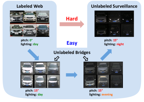
Figure 1: Unsupervised domain adaptation is challenging when the target domain is significantly different from the source domain due to many convoluted factors of variation. We introduce bridging domains composed of unlabeled images with some common factors to the source (e.g., lighting) and the target domain (e.g., viewpoint, image resolution).

Figure 1 provides an illustrative example of adapting from labeled images of cars from the internet to recognize cars for surveillance applications at night. Two dominant factors, the perspective and illumination, make this a difficult adaptation task. As a step towards solving these problems, we introduce unlabeled domain bridges whose factors of variation are partially shared with the source domain, while the others are in common with the target domain. As in Figure 1, the domain on the bottom left shares a consistent lighting condition (day) with the source, while the viewpoint is similar to that of the target domain. We note that there could be multiple bridging domains, such as the one on the bottom right of Figure 1, whose lighting intensity is between that of the first bridging domain and the target domain.

To utilize unlabeled bridging domains, we propose to extend the domain adversarial neural network [Ganin et al.(2016)Ganin, Ustinova, Ajakan, Germain, Larochelle, Laviolette, Marchand, and Lempitsky] using multiple domain discriminators, each of which accounts for learning and reducing the discrepancy between unlabeled (bridging, target) domains and the mix of all precedent domains. We justify our learning framework by deriving a bound on the target error, that contains the source error and a list of discrepancies between unlabeled domain and the mix of precedent domains, including the source. This bound captures the intuition that judicious choices of bridge domains should not introduce large discrepancies. We hypothesize that the decomposition of a single, large discrepancy into multiple, small ones leads to a series of easier optimization problems, culminating in better alignment of source and target domains. We illustrate this intuition in Figure 2 on a variant of the two-moons dataset.

While works on unsupervised discovery of latent domains exist [Gopalan et al.(2011)Gopalan, Li, and Chellappa, Gong et al.(2013)Gong, Grauman, and Sha, Gong et al.(2014)Gong, Grauman, and Sha], it still remains a hard, unsolved problem. Firstly, we focus on the complementary and also unsolved problem of devising adversarial formulations that exploit given bridging domains. We observe that such domain information is often easily available in practice, for example, image meta-data such as timestamps, geo-tags and calibration parameters suffice to inform about illumination, weather or perspective. Moreover, we exploit different methods on measuring domain discrepancy [Gretton et al.(2012)Gretton, Borgwardt, Rasch, Schölkopf, and Smola, Ganin et al.(2016)Ganin, Ustinova, Ajakan, Germain, Larochelle, Laviolette, Marchand, and Lempitsky] or out-of-distribution (OOD) sample detection [Hendrycks and Gimpel(2017)] to discover latent domains in an unsupervised manner, i.e., without domain information.

2 Related Work

Unsupervised Domain Adaptation. The proper reduction of discrepancy across domains [Pan et al.(2010)Pan, Yang, et al.] is a longstanding challenge. Specifically, an appropriate metric is required in order to measure the difference in between domains [Ben-David et al.(2007)Ben-David, Blitzer, Crammer, and Pereira]. Recent works use kernel-based methods such as maximum mean discrepancy (MMD) [Tzeng et al.(2015)Tzeng, Hoffman, Darrell, and Saenko] and optimal transport (OT) [Courty et al.(2015)Courty, Flamary, Tuia, and Rakotomamonjy] to measure the domain difference in the feature space. Others adopt the idea of adversarial training [Ganin et al.(2016)Ganin, Ustinova, Ajakan, Germain, Larochelle, Laviolette, Marchand, and Lempitsky, Sohn et al.(2017)Sohn, Liu, Zhong, Yu, Yang, and Chandraker] which is inspired by the generative adversarial network (GAN) [Goodfellow et al.(2014)Goodfellow, Pouget-Abadie, Mirza, Xu, Warde-Farley, Ozair, Courville, and Bengio]. This training procedure allows the feature representations to be indistinguishable between the source and target domain, aligning the two. One example of using adversarial training on UDA problems is the domain adversarial neural network (DANN) [Ganin et al.(2016)Ganin, Ustinova, Ajakan, Germain, Larochelle, Laviolette, Marchand, and Lempitsky]. It trains a discriminator that distinguishes domains, while also learning a feature extractor to fool the discriminator by providing domain-invariant feature.

Multiple Domains. In [Zhao et al.(2018)Zhao, Zhang, Wu, Moura, Costeira, and Gordon], models are proposed for multiple-source UDA problems based on a domain adversarial learning. While the intuition is to utilize extra source domains that are available, the adaptation process is in practice favored toward the source domain that is closely related to the target domain [Mansour et al.(2009)Mansour, Mohri, and Rostamizadeh]. Our method shares the similar high-level idea, in which relevant domains should guide the adaptation. In contrast, unlabeled bridging domains that share factors of variation with both source and target domains are utilized to guide the two domains, aligned with the bridging domain. Similar to our proposed approach, the benefit of having intermediate domains to guide transfer learning is shown in [Tan et al.(2015)Tan, Song, Zhong, and Yang], but in the context of semi-supervised label propagation, requiring labeled data from the target domains.

3 Method

Our proposed domain adaptation framework is built atop DANN, utilizing unlabeled bridging domains to enhance the adaptation performance when the source and target domains are significantly different due to factors of variations.

Notation. Denote $\mathcal{D}_{S}$ and $\mathcal{D}_{T}$ as the source and target domains, respectively, from which data $x$ are drawn. Output label $y\,{\sim}\,\mathcal{Y}$ has $N$ categories. The model contains: 1) a feature extractor $f\,{:}\,\mathcal{D}\,{\rightarrow}\,\mathbb{R}^{K}$, with parameter $\theta_{f}$, that maps $x$ into a feature vector $f(x)$; 2) the domain discriminator $d\,{:}\,\mathbb{R}^{K}\,{\rightarrow}\,(0,1)$, with parameter $\theta_{d}$, that tells whether $f(x)$ is from $\mathcal{D}_{S}$ or $\mathcal{D}_{T}$; and 3) the classifier $C\,{:}\,\mathbb{R}^{K}\,{\rightarrow}\,\mathcal{Y}$, with parameter $\theta_{C}$, that gives a predicted label $\hat{y}\,{=}\,C(f(x))$.

3.1 Domain Adversarial Neural Network

The domain adversarial neural network transfers a classifier learned from the labeled source domain to the unlabeled target domain by learning domain-invariant features. It is realized by first learning the domain-related information and leveraging it with features extracted from the input. DANN uses a domain discriminator $d$ to control the amount of domain-related information in the extracted feature. The discriminator is updated by maximizing the following:

$$\mathcal{L}_{d}=\mathbb{E}_{x\sim\mathcal{D}_{S}}\log d(f(x))+\mathbb{E}_{x\sim\mathcal{D}_{T}}\log(1-d(f(x))).$$ (1)

In comparison, the feature extractor $f$ wants to confuse the discriminator $d$ to remove any domain-specific information. Moreover, to make sure the extracted feature is task-related, $f$ is trained to generate features that can be correctly classified by the classifier $C$ trained by minimizing the following:

$$\mathcal{L}_{C}=\mathbb{E}_{(x,y)\sim\mathcal{D}_{S}{\times}\mathcal{Y}}[-y\log C(f(x))],$$ (2)

and a learning objective for feature extractor is as follows:

$$\min_{\begin{subarray}{c}\theta_{f},\theta_{C}\end{subarray}}\mathcal{L}_{C}+\lambda\mathcal{L}_{d}.$$ (3)

While [Ganin et al.(2016)Ganin, Ustinova, Ajakan, Germain, Larochelle, Laviolette, Marchand, and Lempitsky] introduces a gradient reversal layer to jointly train all parameters, we do alternating update of GANs [Goodfellow et al.(2014)Goodfellow, Pouget-Abadie, Mirza, Xu, Warde-Farley, Ozair, Courville, and Bengio] between $\theta_{d}$ and $\{\theta_{f},\theta_{C}\}$ in our implementation.

3.2 Challenge in Domain Adversarial Learning

While deep domain adaptation algorithms are realized in different forms [Tzeng et al.(2015)Tzeng, Hoffman, Darrell, and Saenko, Tzeng et al.(2014)Tzeng, Hoffman, Zhang, Saenko, and Darrell, Ganin et al.(2016)Ganin, Ustinova, Ajakan, Germain, Larochelle, Laviolette, Marchand, and Lempitsky, Sohn et al.(2017)Sohn, Liu, Zhong, Yu, Yang, and Chandraker, Bousmalis et al.(2016)Bousmalis, Trigeorgis, Silberman, Krishnan, and Erhan, Su et al.(2020)Su, Tsai, Sohn, Liu, Maji, and Chandraker], their theoretical motivation largely derives from the seminal work of [Ben-David et al.(2007)Ben-David, Blitzer, Crammer, and Pereira]. In short, a theorem from that work states that the target domain task error $\epsilon_{T}$ is bounded by the source error $\hat{\epsilon}_{S}$ and the domain discrepancy:

$$\vspace{-1.4mm}\epsilon_{T}(h)\leq\hat{\epsilon}_{S}(h)+d_{\mathcal{H}\Delta\mathcal{H}}(\mathcal{D}_{S},\mathcal{D}_{T}),$$ (4)

where $h\,{\in}\,\mathcal{H}$ is a hypothesis and $d_{\mathcal{H}\Delta\mathcal{H}}$ is written as:

$$\sup_{h,h^{\prime}\,{\in}\,\mathcal{H}}|P_{\mathcal{D}_{S}}(h(x)\,{\neq}\,h^{\prime}(x))-P_{\mathcal{D}_{T}}(h(x)\,{\neq}\,h^{\prime}(x))|.$$

Adversarial loss can be used to minimize the domain discrepancy to obtain a tighter bound. While it provides flexibility on the types of discrepancy, it is challenging to learn the right transformation from the source domain to the target domain when the two are far apart.

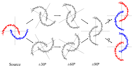
Figure 2: Translated two moons. The inter-twinning moons (left) are considered as the source domain. Two moons are rotated and translated to the right to generate the target domain (right in gray).

As motivation, consider a variant of the two-moons dataset, whose data points are translated to the right by the amount proportional to the rotation angle, as in Figure 2. The source domain is centered at the origin, while the target domain is moved to the right after being rotated by $90^{\circ}$, and given without labels. Adapting from source to target directly is difficult due to a significant change. Moreover, there are many ways to generate the same unlabeled target data points (e.g., rotate counterclockwise instead of clockwise, as in the bottom of Figure 2). In such a case, knowing what happens in the middle of the entire transformation process from source to target domains is critical, as these data points in the middle, even if they are unlabeled, can guide learning algorithms to easily disentangle transformation factors (e.g., clockwise rotation and translation to the right) from task-relevant factors.

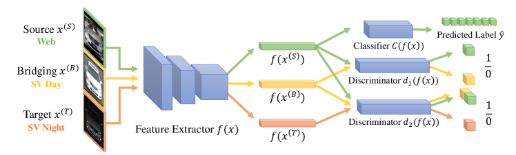
Figure 3: The learning framework with labeled source, unlabeled target, and unlabeled bridging domains for our extension of DANN using multiple discriminators. The model is composed of shared feature extractor $f$, classifier $C$, which is trained using labeled source examples, and two domain discriminators $d_{1}$ and $d_{2}$.

3.3 Adaptation with Bridging Domain

We introduce additional sets of unlabeled examples, which we call bridging domains, that reside in the transformation pathway from labeled source to unlabeled target domains.

DANN with a Single Bridging Domain.

Besides $\mathcal{D}_{S}$ and $\mathcal{D}_{T}$, we denote $\mathcal{D}_{B}$ as a bridging domain. Our framework is composed of feature extractor $f(x)$ from an input $x\,{\in}\,\mathcal{D}_{S}\,{\cup}\,\mathcal{D}_{B}\,{\cup}\,\mathcal{D}_{T}$ and classifier $C(f(x))$ trained using classification loss in (2). Unlike DANN, which directly aligns $\mathcal{D}_{S}$ and $\mathcal{D}_{T}$, we decompose the adaptation into two steps. First, $\mathcal{D}_{S}$ and $\mathcal{D}_{B}$ are aligned. This is an easier task than direct adaptation as in DANN, since there are less discriminating factors between $\mathcal{D}_{S}$ and $\mathcal{D}_{B}$. Second, we adapt $\mathcal{D}_{T}$ to the union of $\mathcal{D}_{S}$ and $\mathcal{D}_{B}$. Similarly, the task is easier since it needs to discover remaining factors between $\mathcal{D}_{T}$ and $\mathcal{D}_{S}$ or $\mathcal{D}_{B}$, as some factors are already found from the previous step. To accommodate the two adaptation steps, we use two binary domain discriminators, $d_{1}$ for learning discrepancy between $\mathcal{D}_{S}$ and $\mathcal{D}_{B}$, and $d_{2}$ between $\mathcal{D}_{S}\,{\cup}\,\mathcal{D}_{B}$ and $\mathcal{D}_{T}$. Finally, this is realized with the following objectives:

$$\mathcal{L}_{d_{1}} \,{=}\;\mathbb{E}_{\mathcal{D}_{S}}\log d_{1}(f)+\mathbb{E}_{\mathcal{D}_{B}}\log(1\,{-}\,d_{1}(f)),$$ (5)

$$\mathcal{L}_{d_{2}} \,{=}\;\mathbb{E}_{\mathcal{D}_{S}\cup\mathcal{D}_{B}}\log d_{2}(f)+\mathbb{E}_{\mathcal{D}_{T}}\log(1\,{-}\,d_{2}(f)).$$ (6)

Both $\mathcal{L}_{d_{1}}$ and $\mathcal{L}_{d_{2}}$ are minimized to update their respective model parameters $\theta_{d_{1}}$ and $\theta_{d_{2}}$. We update the classifier using (2) and the feature extractor to confuse discriminators as follows:

$$\min_{\begin{subarray}{c}\theta_{f},\theta_{C}\end{subarray}}\mathcal{L}_{C}+\lambda_{1}\mathcal{L}_{d_{1}}+\lambda_{2}\mathcal{L}_{d_{2}},$$ (7)

with two hyperparameters $\lambda_{1}$ and $\lambda_{2}$ to adjust the strengths of adversarial loss. We alternate updates between $d_{1},d_{2}$ and $f,C$. The proposed framework is visualized in Figure 3.

Theoretical Insights.

To provide insights on how our learning objectives are constructed, we derive a bound on the target error while considering the unlabeled bridging domain:

$$\epsilon_{T}(h)\leq\epsilon_{T}(h_{T}^{*})+\tfrac{1}{2}\epsilon_{B}(h_{B}^{*})+2\gamma_{\alpha}+\eta+d_{\mathcal{H}\Delta\mathcal{H}}(\mathcal{D}_{\alpha},\mathcal{D}_{T})+\tfrac{1}{2}d_{\mathcal{H}\Delta\mathcal{H}}(\mathcal{D}_{S},\mathcal{D}_{B}),$$ (8)

where $h^{*}\,{=}\,\arg{\min}_{h\in\mathcal{H}}\epsilon(h)$, $\mathcal{D}_{\alpha}\,{=}\,\mathcal{D}_{S}\,{\cup}\,\mathcal{D}_{B}$, and

$$\gamma_{\alpha}\,{=}\,{\textstyle\min}_{h\in\mathcal{H}}\{\epsilon_{T}(h)\,{+}\,{\textstyle\sum}_{j=1}^{N}\alpha_{j}\epsilon_{j}(h)\}\text{ with $\alpha{=}(0.5,0.5)$.}$$

Note that $\epsilon_{T}(h_{T}^{*}){+}\tfrac{1}{2}\epsilon_{B}(h_{B}^{*}){+}2\gamma_{\alpha}{\approx}\hat{\epsilon}_{S}(h)$, making (8) similar to (4). The derivation is provided in the Supplementary Material.

The implications of (8) are two-fold: Firstly, to keep the bound tight, we need to assure that both domain discrepancies are small. This motivates the design of our proposed adversarial learning framework discussed earlier. More importantly, we argue that the individual components of decomposed discrepancies are much easier to optimize than the one in (4) when the bridging domain is chosen properly.

Unsupervised Bridging Domain Discovery.

While there are many real-world problems where the bridging domains naturally arise (e.g., the illumination condition of the surveillance images, which can be obtained from the mean pixel values), it is not always available. In such cases, one may resort to the unsupervised discovery of latent domains [Gopalan et al.(2011)Gopalan, Li, and Chellappa, Gong et al.(2013)Gong, Grauman, and Sha, Tan et al.(2015)Tan, Song, Zhong, and Yang].

To find out whether an unlabeled image of the target domain belongs to the bridging domain, one may measure the closeness of individual target examples to the source domain. For example, we propose to pretrain a standard DANN and exploit the discriminator score $d_{\text{pre}}(f_{\text{pre}}(x)),x\,{\in}\,\mathcal{D}_{T}$ to quantify the closeness. Since the discriminator converges at equilibrium of source and target distributions [Goodfellow et al.(2014)Goodfellow, Pouget-Abadie, Mirza, Xu, Warde-Farley, Ozair, Courville, and Bengio], this requires an early stopping in practice [Sohn et al.(2017)Sohn, Liu, Zhong, Yu, Yang, and Chandraker].

Alternatively, we can use off-the-shelf algorithms to compute the distance between individual target examples to the source domain. Given a feature extractor $f_{\text{pre}}$ trained on the source examples, one may compute the MMD between $f_{\text{pre}}(x),x\,{\in}\,\mathcal{D}_{T}$ and $\{f_{\text{pre}}(x)\}_{x\,{\in}\,\mathcal{D}_{S}}$. In addition, out-of-distribution (OOD) sample detection methods [Hendrycks and Gimpel(2017)] are good candidates as they provide the score quantifying how likely an example belongs to the source domain.

DANN with Multiple Bridging Domains.

Our framework can be extended to the case for which multiple unlabeled bridging domains exist, which is desirable to span larger discrepancies between source and target domains. To formalize, we denote $\mathcal{D}_{0}\,{=}\,\mathcal{D}_{S},\mathcal{D}_{M{+}1}\,{=}\,\mathcal{D}_{T}$ as source and target domains, and $\mathcal{D}_{m},\,m\,{=}\,1,...,M$ as unlabeled bridging domains with $\mathcal{D}_{m}$ closer to source than $\mathcal{D}_{m{+}1}$. We introduce $M{+}1$ domain discriminators $d_{1},...,d_{M{+}1}$, each of which is trained by maximizing the following objective:

$$\mathcal{L}_{d_{m}}\,{=}\;\mathbb{E}_{\bigcup_{i=0}^{m{-}1}\mathcal{D}_{i}}\log d_{m}(f)+\mathbb{E}_{\mathcal{D}_{m}}\log(1\,{-}\,d_{m}(f)),$$ (9)

and the learning objective for $f$ and $C$ is given as follows:

$$\min_{\begin{subarray}{c}\theta_{f},\theta_{C}\end{subarray}}\mathcal{L}_{C}+{\textstyle\sum}_{m=1}^{M+1}\lambda_{m}\mathcal{L}_{d_{m}}.$$ (10)

4 Experiments

We evaluate our methods mainly on three adaptation tasks: digit classification, object recognition, and semantic scene segmentation. For the recognition task, we use the Comprehensive Cars (CompCars) [Yang et al.(2015)Yang, Luo, Change Loy, and Tang] dataset to recognize car models in the surveillance domain at night using labeled images from the web domain. For the scene segmentation task, synthetic images of the GTA5 dataset [Richter et al.(2016)Richter, Vineet, Roth, and Koltun] are given as the source domain and the task is to perform adaptation on Foggy Cityscapes [Sakaridis et al.(2018)Sakaridis, Dai, and Van Gool]. In the Supplementary Material, we provide more results on the two-moons toy dataset as described previously and the digit classification task.

4.1 Toy Experiment with Two Moons

Created for binary classification problem, the inter-twinning moons 2D dataset suits our model if we consider different rotated versions of the standard two entangled moons as different domains. In this experiment, we consider a hard adaptation from the original data to the ones that are rotated $90^{\circ}$ (clockwise or counter-clockwise), while intermediate rotation such as $30^{\circ}$ and $60^{\circ}$ can be considered as bridging domains. Moreover, as discussed in Section 3.2, the domains do not share the same centers and are proportionally translated according to the rotated angle. We follow the same network architecture as in [Ganin et al.(2016)Ganin, Ustinova, Ajakan, Germain, Larochelle, Laviolette, Marchand, and Lempitsky], with one hidden layer of $15$ neurons followed by sigmoid non-linearity. The performance is summarized in Table 1.

Model	$0^{\circ}$	$30^{\circ}$	$60^{\circ}$	$90^{\circ}$
0$\to$90	80.88$\pm$1.71	-	-	56.98$\pm$4.47
0$\to$30$\to$90	87.23$\pm$3.64	95.66$\pm$4.18	-	60.98$\pm$7.41
0$\to$60$\to$90	79.19$\pm$1.21	-	89.66$\pm$3.61	80.67$\pm$9.47
0$\to$30$\to$60$\to$90	78.75$\pm$1.56	82.33$\pm$8.71	87.33$\pm$3.83	86.97$\pm$2.17

Table 1: Average classification accuracy on test set of each domain. Results for the baseline and different bridging domain combinations are included.

One observation is that when $90^{\circ}$ is involved as a target domain, the source domain accuracy is sacrificed a lot, which may be because of the limited network capacity. While the adaptation achieves only $56.90\%$, which is almost a random guess, with source-to-target model ($0{\to}90$), the proposed method clearly demonstrates its effectiveness, achieving $86.97\%$ on the target domain.

4.2 Digit Classification

Different digit datasets are considered as separated domains. MNIST [LeCun et al.(1998)LeCun, Bottou, Bengio, and Haffner] provides a large amount of hand written digit images in gray scale. SVHN [Netzer et al.(2011)Netzer, Wang, Coates, Bissacco, Wu, and Ng] contains colored digit images of house numbers from street view. MNIST-M [Ganin et al.(2016)Ganin, Ustinova, Ajakan, Germain, Larochelle, Laviolette, Marchand, and Lempitsky] is enriched from MNIST using randomly selected colored image patches in BSD500 [Arbelaez et al.(2011)Arbelaez, Maire, Fowlkes, and Malik] as background. We consider adaptation from labeled MNIST to unlabeled SVHN, while using MNIST-M as an unlabeled bridging domain. Given the differences between MNIST and SVHN, MNIST-M seems appropriate bridging domain (similar appearance of foreground digits to MNIST but color statistics to SVHN).

Model	MNIST-M	SVHN
MNIST$\to$SVHN	-	71.02
MNIST$\to$MNIST-M$+$SVHN	96.27	78.07
MNIST$\to$MNIST-M$\to$SVHN	97.07	81.28

Table 2: Accuracy on MNIST-M and SVHN test sets averaged over 10 runs. We report the performance of the standard DANN, the DANN model using mixture of unlabeled domains as a single target (MNIST$\to$MNIST-M$+$SVHN), and our proposed model.

We compare our model with the baseline model, i.e., a standard DANN from source to target without bridging domain. A DANN model that adapts to the mixture of bridge and target domains as a single target is included for comparison. We present results in Table 2. When the bridging domain is involved, the average accuracy on SVHN (target) significantly improves upon the baseline model. Moreover, our proposed model achieves higher performance than the model with mixture of unlabeled domains, demonstrating benefits from the bridging domain.

4.3 Recognizing Cars in SV Domain at Night

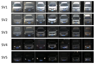
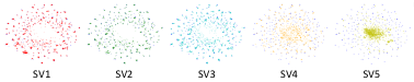
Figure 4: Sample images of CompCars surveillance (SV) domain from light (SV1) to dark (SV5) illumination conditions.

Figure 5: t-SNE plots of CompCars web and SV domains from light (SV1) to dark (SV5) illumination conditions using baseline features.

Dataset and Experimental Setting.

Two sets of images are provided in the CompCars dataset: 1) the web-nature images are collected from car forums, public websites and search engines, and 2) the surveillance-nature images are collected from surveillance cameras. The dataset is composed of $52,083$ web images across $431$ car models and $44,481$ SV images across $181$ car models, with these categories of the SV set being inclusive of $431$ categories from the web set. We consider a set of adaptation problems from labeled web to unlabeled SV images. This is challenging as SV images have different perspective and illumination variations from web images.

We use an illumination condition as a metric for adaptation difficulty and partition the SV set into SV1–5 based on the illumination condition of each image. SV1 contains the brightest images, whereas SV5 contains the darkest ones. We visualize samples from SV1–5 in Figure 5, and confirm the domain discrepancy between web and SV1–5 domains through t-SNE plots in Figure 5. More details of model architecture and training are in the Supplementary Material.

We present two experimental protocols. First, we evaluate on an adaptation task from web to SV night (SV4–5) using SV day (SV1–3) as one domain bridge. We demonstrate the difficulty of adaptation when two domains are far from each other, and show the importance of bridging domain and the effectiveness our adaptation method. Second, we adapt to extreme SV domain (SV5) using different combinations of one or multiple bridging domains (SV1–4) and characterize the properties of an effective bridging domain.

Evaluation with a Single Bridging Domain.

We demonstrate the difficulty of adaptation when domains are far apart and show that the performance of adversarial DA can be enhanced using bridging domains. In particular, night images (SV4–5) are considered as unlabeled target domain and day images (SV1–3) as unlabeled bridging domain. We compare the following models in Table 3: baseline model trained on labeled web images, DANN from source to target (Web$\to$SV4–5), from source to mixture of bridge and target (Web$\to$SV1–5), and the proposed model from source to bridge to target (Web$\to$SV1–3$\to$SV4–5).

Model	SV1–3	SV4–5
Web (source only)	72.67	19.87
Web$\to$SV4–5	68.90$\pm$1.28	49.83$\pm$0.70
Web$\to$SV4$\to$5	74.03$\pm$0.71	61.37$\pm$0.30
Web$\to$SV1–5	83.29$\pm$0.14	77.84$\pm$0.34
Web$\to$SV1–3$\to$4–5	82.83$\pm$0.40	78.78$\pm$0.33

Table 3: Accuracy and standard error over 5 runs on SV test sets for models without (Web$\to$SV4–5) and with (Web$\to$SV4$\to$5, Web$\to$SV1–3$\to$4–5) bridging domain. Baselines include a model using mixture of bridge and target domains as a single target domain (Web$\to$SV1–5).

While the DANN adapted to the target domain (SV4–5) improves upon the baseline model, the performance is still far from adequate when compared to the performance of day images. By introducing unlabeled bridging domain, we observe significant improvement in accuracy on the target domain, achieving $77.84\%$ using standard DANN adapted to the mixture of bridging and target domains and $78.78\%$ using our proposed method.

We further conduct an experiment using SV4 as a bridge domain and SV5 as a target domain and compare with the naively trained model (Web$\to$SV4–5). As in Table 3, the proposed model (Web$\to$SV4$\to$5) outperforms the DANN by a large margin ($49.83\%$ to $61.37\%$ on SV4–5 test set). This is because it is difficult to determine the adaptation curriculum as both domains are distant from the source domain (see Figure 5), which is different from the previous experiment where there are sufficient amount of day images that are fairly close to the source domain, for discriminator to figure out the curriculum.

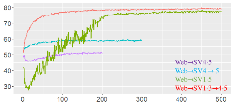
Figure 6: Validation accuracy on SV4–5 (night)

To better understand the advantage of our proposed training scheme, we monitor the validation accuracy on SV4–5 of the standard (Web$\to$SV1–5) and the proposed (Web$\to$SV1–3$\to$4–5) models and plot curves in Figure 6. Interestingly, we observe a large fluctuation in the performance of night images using the standard DANN. In contrast, our method allows stable performance earlier in the training, which implies that knowing the curriculum [Bengio et al.(2009)Bengio, Louradour, Collobert, and Weston] ($i.e.$, adaptation difficulty) is important. Our method with multiple discriminators effectively utilizes such information.

Model	SV5
Web$\to$SV5	37.83$\pm$0.51
Web$\to$SV4$\to$5	58.40$\pm$0.60
Web$\to$SV1$\to$5	69.69$\pm$0.99
Web$\to$SV3$\to$4$\to$5	74.01$\pm$0.52
Web$\to$SV2$\to$3$\to$4$\to$5	75.15$\pm$0.18
Web$\to$SV1$\to$2$\to$3$\to$4$\to$5	75.47$\pm$0.20

Table 4: Accuracy and standard error over 5 runs on SV5 test set.

Split	OOD (0.69)	MMD (0.79)	$d$-Score (0.85)
2-way	76.43$\pm$0.28	78.32$\pm$0.27	78.62$\pm$0.39
3-way	76.14$\pm$0.34	78.47$\pm$0.31	78.29$\pm$0.28
4-way	76.67$\pm$0.32	78.68$\pm$0.39	77.93$\pm$0.43
5-way	76.54$\pm$0.29	78.91$\pm$0.33	79.13$\pm$0.32

Table 5: Accuracy and standard error over 5 runs on SV4–5 test set with different unsupervised bridging domain discovery configurations. Split $m$-way means that we evenly split the unlabeled data into $m$ domains.

Which is a Good Bridging Domain?

We perform an ablation study to characterize the properties of a good bridging domain. Specifically, we would like to answer which is a more useful bridging domain: the one closer to the source domain or the one closer to the target domain. To this end, we compare two models, namely, Web$\to$SV1$\to$5 and Web$\to$SV4$\to$5. Note that SV4 is more similar to the target domain (SV5) in terms of visual attributes than SV1.

The results are summarized in Table 5. We observe much higher accuracy on the target domain (SV5) for the model using SV1 as a bridging domain ($69.69\%$) than the one using SV4 ($58.40\%$). We believe that the optimization of the adversarial loss for the second model ($d_{\mathcal{H}\Delta\mathcal{H}}(\text{W},\text{SV4})+d_{\mathcal{H}\Delta\mathcal{H}}(\text{W}{+}\text{SV4},\text{SV5})$) is more difficult than that of the first model ($d_{\mathcal{H}\Delta\mathcal{H}}(\text{W},\text{SV1})\,{+}\,d_{\mathcal{H}\Delta\mathcal{H}}(\text{W}{+}\text{SV1},\text{SV5})$) as SV4 is farther from the web domain than SV1. This implies that a good bridging domain decomposes the domain discrepancy between the source and target domains, so that the decomposed discrepancy losses is easily optimized.

Evaluation with Multiple Bridging Domains.

Our theoretical motivation suggests that, if we have many bridging domains whose generalization error between any two neighboring domains is small, we can also reduce the generalization error between source and target.

We test our hypothesis through experiments that adapt to SV5 with different bridging domain configurations. Specifically, bridging domains are included one by one from SV4 to SV1, and finally reach adaptation with four bridging domains. As in shown Table 5, DANN fails at adaptation without domain bridge (Web$\to$SV5). While including SV4 as the target domain raises adaptation difficulty, using it as a bridging domain (Web$\to$SV4$\to$5) greatly improves the performance on the SV5 test set. Including SV3 as an additional bridging domain (Web$\to$SV3$\to$4$\to$5) shows additional improvement, confirming our hypothesis. While adding SV2 and SV1 as bridging domains leads to an extra improvement, the margin is not as large as including SV3 and SV4. The reason is that SV3 is already close to the web domain as SV1 or SV2 (see Figure 5 and 5), and there is little benefit of introducing an extra bridge.

Evaluation with Unsupervised Bridge Discovery.

We perform several unsupervised approaches for bridging domain discovery, including discriminator scores of the DANN, MMD, and OOD sample detection [Hendrycks and Gimpel(2017)]. These approaches provide scores indicating the closeness to the source domain distribution for each target example, based on which we can split the target domain into multiple bridging domains (details in the Supplementary Material).

To evaluate the performance of our methods on unsupervised bridging domain discovery, we first compute the AUC between the predicted score and the ground-truth day/night labels and report results in Table 5. While we observe the highest AUC using discriminator of the DANN ($0.85$), it requires early stopping based on the AUC. In comparison, MMD ($0.79$) and OOD ($0.69$) show slightly lower AUC, but are preferred as additional side information is not required. Overall, we observe that using $d$-Score or MMD, the performance on SV4–5 test set is improved compared to not using any domain bridges (Table 3 Web$\to$SV1–5).

4.4 Foggy Scene Segmentation

Dataset and Experimental Setting.

We use the GTA5 dataset [Richter et al.(2016)Richter, Vineet, Roth, and Koltun], a synthetic dataset of street-view images, containing 24,966 images of size $1914{\times}1052$, as labeled source domain. Unlike previous works [Hoffman et al.(2016)Hoffman, Wang, Yu, and Darrell, Tsai et al.(2018)Tsai, Hung, Schulter, Sohn, Yang, and Chandraker], we adapt to Foggy Cityscapes [Sakaridis et al.(2018)Sakaridis, Dai, and Van Gool], a derivative from the real scene images of Cityscapes [Cordts et al.(2016)Cordts, Omran, Ramos, Rehfeld, Enzweiler, Benenson, Franke, Roth, and Schiele] with a fog simulation, and use Cityscapes as well as Foggy Cityscapes with lighter foggy levels ($0.01$) as unlabeled bridging domains.

The task is to categorize each pixel into one of 19 semantic categories on the test set images of Foggy Cityscapes with $0.02$ foggy level. We consider several models for comparison, such as the traditional DANN (GTA5${\to}\text{F}_{0.02}$), with one bridging domain (GTA5${\to}\text{City}{\to}\text{F}_{0.02}$), or with two of them (GTA5${\to}\text{City}{\to}\text{F}_{0.01}{\to}\text{F}_{0.02}$). One consideration is that we partition $2975$ training images of Cityscapes equally for each domain to prevent the case where the algorithm finds an exact correspondence between images from different unlabeled domains.

Evaluation on Semantic Segmentation.

We utilize the adaptation method by [Tsai et al.(2018)Tsai, Hung, Schulter, Sohn, Yang, and Chandraker] as our base model, which reduces the domain discrepancy at structured output spaces. The same discriminator architecture is used for multiple adversarial losses in our framework.

Model	# images	mIoU on $\text{F}_{0.02}$
GTA5 (source only)	–	27.5
GTA5${\rightarrow}\text{F}_{0.02}$ [Tsai et al.(2018)Tsai, Hung, Schulter, Sohn, Yang, and Chandraker]	$1487$	33.08$\pm$0.32
GTA5${\rightarrow}\text{City}{+}\text{F}_{0.02}$		32.62$\pm$0.58
GTA5${\rightarrow}\text{City}{\rightarrow}\text{F}_{0.02}$		34.82$\pm$0.39
GTA5${\rightarrow}\text{F}_{0.02}$ [Tsai et al.(2018)Tsai, Hung, Schulter, Sohn, Yang, and Chandraker]	$991$	33.16$\pm$0.35
GTA5${\rightarrow}\text{City}{\rightarrow}\text{F}_{0.02}$		34.13$\pm$0.78
GTA5${\rightarrow}\text{City}{\rightarrow}\text{F}_{0.01}{\rightarrow}\text{F}_{0.02}$		35.31$\pm$0.06

Table 6: mIoU and standard error over 5 runs on Foggy Cityscapes $0.02$ ($\text{F}_{0.02}$) test set. We partition unlabeled training data into 2 for models in rows 2–4, resulting in $1487$ images per domain, while for models in rows 5–7, we partition them into 3, resulting in $991$ images per domain.

We first conduct experiments with one bridging domain to adapt to Foggy Cityscapes $0.02$ ($\text{F}_{0.02}$). We construct two partitions of unlabeled data for Cityscapes and $\text{F}_{0.02}$. Mean intersection-over-union (IoU) averaged over 5 runs, using different partition for each run, is reported in rows 2–4 of Table 6. While significant improvement in mIoU is observed by directly adapting to the target domain (GTA5${\to}\text{F}_{0.02}$), our framework using a bridging domain further enhances the performance on the final target domain from $33.08$ to $34.82$. We also conduct a baseline model by merging Cityscapes with the target domain (GTA5${\to}\text{City}{+}\text{F}_{0.02}$), but the performance is not good, indicating that naively merging two domains with different properties may be suboptimal for adversarial adaptation.

We then experiment with two bridging domains by introducing Foggy Cityscapes $0.01$ ($\text{F}_{0.01}$) as a bridge between Cityscapes and $\text{F}_{0.02}$. The setting is similar, but we use $\tfrac{1}{3}$ of entire images for each unlabeled domain. Table 6 rows 5–7 validate our hypothesis that additional bridging domains are beneficial, improving mIoU from $34.13$ to $35.31$. While using the same number of overall unlabeled images during the training, we also observe benefit of using two bridging domains ($7^{\text{th}}$ row) than one ($4^{\text{th}}$ row).

5 Conclusions

This paper aims to simplify adaptation problems with extreme domain variations, using unlabeled bridging domains. A novel framework based on DANN is developed by introducing additional discriminators to account for decomposed many, but smaller discrepancies of the source-to-target domain discrepancy. Several adaptation tasks in computer vision are considered, demonstrating the effectiveness of our framework with bridging domains.

S1 Proof of (8)

With source and bridging domains, $h^{*}\,{=}\,\arg\min_{h\in\mathcal{H}}\epsilon(h)$, $h_{1}\,{=}\,\arg\min_{h\in\mathcal{H}}\hat{\epsilon}_{S}(h)$, an empirical minimizer of source error, and weight vector $\alpha\,{=}\,(0.5,0.5)$, for any $\delta\in(0,1)$, with probability at least $1-\delta$, the target error can be bounded as follows:

$$\begin{split}\epsilon_{T}(h_{1})&\leq\epsilon_{T}(h_{T}^{*})+\tfrac{1}{2}\epsilon_{B}(h_{B}^{*})+2\gamma+2\eta\\ &+d_{\mathcal{H}\Delta\mathcal{H}}(\mathcal{D}_{\alpha},\mathcal{D}_{T})+\tfrac{1}{2}d_{\mathcal{H}\Delta\mathcal{H}}(\mathcal{D}_{S},\mathcal{D}_{B})\end{split}$$ (S1)

where $h\in\mathcal{H}$ is a hypothesis and

$$d_{\mathcal{H}\Delta\mathcal{H}} =\sup_{h,h^{\prime}\,{\in}\,\mathcal{H}}|P_{\mathcal{D}_{S}}(h(x)\,{\neq}\,h^{\prime}(x))-P_{\mathcal{D}_{T}}(h(x)\,{\neq}\,h^{\prime}(x))|$$ (S2)

$$\gamma =\min_{h\in\mathcal{H}}\epsilon_{T}(h)+\epsilon_{S}(h)+\epsilon_{B}(h)$$ (S3)

$$\eta =2\sqrt{\left(\frac{2d\log(2m+1)+\log(\tfrac{4}{\delta})}{m}\right)}$$ (S4)

Proof.

For the presentation clarity, we use $\epsilon_{\alpha}=\tfrac{1}{2}\epsilon_{S}+\tfrac{1}{2}\epsilon_{B}$ interchangeably. Let $h_{1},h_{2},h_{3}\in\mathcal{H}$, which will be defined later. We begin by bounding the target error $\epsilon_{T}$ by the mixture error $\epsilon_{\alpha}$ and the divergence as follows:

$$\epsilon_{T}(h_{1})\leq\epsilon_{T}(h_{2})+\epsilon_{\alpha}(h_{1},h_{2})+\tfrac{1}{2}d_{\mathcal{H}\Delta\mathcal{H}}(D_{\alpha},D_{T})$$ (S5)

The second term of RHS in (S5) is further bounded as follows:

$$\epsilon_{\alpha}(h_{1},h_{2}) =\tfrac{1}{2}\epsilon_{S}(h_{1},h_{2})+\tfrac{1}{2}\epsilon_{B}(h_{1},h_{2})$$ (S6)

$$\leq\tfrac{1}{2}\big{[}\epsilon_{S}(h_{1})+\epsilon_{S}(h_{2})\big{]}+\tfrac{1}{2}\big{[}\epsilon_{B}(h_{1})+\epsilon_{B}(h_{2})\big{]}$$ (S7)

and $\epsilon_{B}(h_{1})$ is bounded as follows:

$$\epsilon_{B}(h_{1}) \leq\epsilon_{B}(h_{3})+\epsilon_{S}(h_{1},h_{3})+\tfrac{1}{2}d_{\mathcal{H}\Delta\mathcal{H}}(D_{S},D_{B})$$ (S8)

$$\leq\epsilon_{B}(h_{3})+\epsilon_{S}(h_{1})+\epsilon_{S}(h_{3})+\tfrac{1}{2}d_{\mathcal{H}\Delta\mathcal{H}}(D_{S},D_{B})$$ (S9)

Plugging (S7) and (S9) into (S5), we get the following:

$$\epsilon_{T}(h_{1}) \leq\epsilon_{T}(h_{2})+\Big{[}\tfrac{1}{2}\big{[}\epsilon_{S}(h_{1})+\epsilon_{S}(h_{2})\big{]}+\tfrac{1}{2}\big{[}\epsilon_{B}(h_{1})+\epsilon_{B}(h_{2})\big{]}\Big{]}+\tfrac{1}{2}d_{\mathcal{H}\Delta\mathcal{H}}(D_{\alpha},D_{T})$$ (S10)

$$=\big{[}\epsilon_{T}(h_{2})+\tfrac{1}{2}\epsilon_{S}(h_{2})+\tfrac{1}{2}\epsilon_{B}(h_{2})\big{]}+\tfrac{1}{2}\big{[}\epsilon_{B}(h_{3})+\epsilon_{S}(h_{3})\big{]}+\epsilon_{S}(h_{1})$$

$$\qquad\qquad\qquad\qquad\qquad\qquad+\tfrac{1}{2}d_{\mathcal{H}\Delta\mathcal{H}}(D_{\alpha},D_{T})+\tfrac{1}{4}d_{\mathcal{H}\Delta\mathcal{H}}(D_{S},D_{B})$$ (S11)

Assuming $h_{2}=\arg\min_{h}\{\epsilon_{T}(h)+\tfrac{1}{2}\epsilon_{S}(h)+\tfrac{1}{2}\epsilon_{B}(h)\}$ and $h_{3}=\arg\min_{h}\{\epsilon_{B}(h)+\epsilon_{S}(h)\}$, the RHS of (S11) is written as follows:

$$\epsilon_{T}(h_{1})\leq\gamma_{1}+\tfrac{1}{2}\gamma_{2}+\epsilon_{S}(h_{1})+\tfrac{1}{2}d_{\mathcal{H}\Delta\mathcal{H}}(D_{\alpha},D_{T})+\tfrac{1}{4}d_{\mathcal{H}\Delta\mathcal{H}}(D_{S},D_{B})$$ (S12)

where $\gamma_{1}=\min_{h}\{\epsilon_{T}(h)+\tfrac{1}{2}\epsilon_{S}(h)+\tfrac{1}{2}\epsilon_{B}(h)\}$ and $\gamma_{2}=\min_{h}\{\epsilon_{B}(h)+\epsilon_{S}(h)\}$. We further assume that $h_{1}=\arg\min_{\hat{\epsilon}_{S}(h)}$, an empirical minimizer of source error.

Now we are left with bounding the source error $\epsilon_{S}(h_{1})$ by the empirical source error $\hat{\epsilon}_{S}(h_{1})$, theoretical minimum errors of the target $\epsilon_{T}(h_{T}^{*})$ and the bridging $\epsilon_{B}(h_{B}^{*})$ domains. This is done by using Lemma 6 in [Ben-David et al.(2010)Ben-David, Blitzer, Crammer, Kulesza, Pereira, and Vaughan] as follows:

$$\epsilon_{S}(h_{1}) \leq\hat{\epsilon}_{S}(h_{1})+\eta$$ (S13)

$$\leq\tfrac{1}{2}\hat{\epsilon}_{S}(h_{T}^{*})+\tfrac{1}{2}\hat{\epsilon}_{S}(h_{B}^{*})+\eta$$ (S14)

$$\leq\tfrac{1}{2}{\epsilon}_{S}(h_{T}^{*})+\tfrac{1}{2}{\epsilon}_{S}(h_{B}^{*})+2\eta$$ (S15)

$$\leq\tfrac{1}{2}{\epsilon}_{S}(h_{T}^{*})+\tfrac{1}{2}\Big{[}{\epsilon}_{B}(h_{B}^{*})+\underbrace{{\epsilon}_{S}(h_{3})+{\epsilon}_{B}(h_{3})}_{=\gamma_{2}}+\tfrac{1}{2}d_{\mathcal{H}\Delta\mathcal{H}}(D_{S},D_{B})\Big{]}+2\eta$$ (S16)

$$\leq\tfrac{1}{2}{\epsilon}_{S}(h_{T}^{*})+\tfrac{1}{2}{\epsilon}_{B}(h_{B}^{*})+\tfrac{1}{2}\gamma_{2}+\tfrac{1}{4}d_{\mathcal{H}\Delta\mathcal{H}}(D_{S},D_{B})+2\eta$$ (S17)

$$\leq\underbrace{\tfrac{1}{2}{\epsilon}_{S}(h_{T}^{*})+\tfrac{1}{2}{\epsilon}_{B}(h_{T}^{*})}_{=\epsilon_{\alpha}(h_{T}^{*})}+\tfrac{1}{2}{\epsilon}_{B}(h_{B}^{*})+\tfrac{1}{2}\gamma_{2}+\tfrac{1}{4}d_{\mathcal{H}\Delta\mathcal{H}}(D_{S},D_{B})+2\eta$$ (S18)

$$\leq\Big{[}\epsilon_{T}(h_{T}^{*})+\underbrace{\epsilon_{T}(h_{2})+\epsilon_{\alpha}(h_{2})}_{=\gamma_{1}}+\tfrac{1}{2}d_{\mathcal{H}\Delta\mathcal{H}}(D_{\alpha},D_{T})\Big{]}+\tfrac{1}{2}{\epsilon}_{B}(h_{B}^{*})+\tfrac{1}{2}\gamma_{2}+\tfrac{1}{4}d_{\mathcal{H}\Delta\mathcal{H}}(D_{S},D_{B})+2\eta$$ (S19)

$$=\epsilon_{T}(h_{T}^{*})+\tfrac{1}{2}{\epsilon}_{B}(h_{B}^{*})+\gamma_{1}+\tfrac{1}{2}\gamma_{2}+\tfrac{1}{2}d_{\mathcal{H}\Delta\mathcal{H}}(D_{\alpha},D_{T})+\tfrac{1}{4}d_{\mathcal{H}\Delta\mathcal{H}}(D_{S},D_{B})+2\eta$$ (S20)

where the second inequality is due to the fact that $h_{1}=\arg\min_{h}\hat{\epsilon}_{S}$ and sixth is by adding $\tfrac{1}{2}{\epsilon}_{B}(h_{T}^{*})$ to RHS. $\eta$ and $2\eta$ are introduced in the second and third inequalities using Lemma 6. Finally, plugging in (S20) into (S12), we get the following:

$$\epsilon_{T}(h_{1}) \leq\epsilon_{T}(h_{T}^{*})+\tfrac{1}{2}{\epsilon}_{B}(h_{B}^{*})+2\gamma_{1}+\gamma_{2}+d_{\mathcal{H}\Delta\mathcal{H}}(D_{\alpha},D_{T})+\tfrac{1}{2}d_{\mathcal{H}\Delta\mathcal{H}}(D_{S},D_{B})+2\eta$$ (S21)

$$\leq\epsilon_{T}(h_{T}^{*})+\tfrac{1}{2}{\epsilon}_{B}(h_{B}^{*})+2\gamma+d_{\mathcal{H}\Delta\mathcal{H}}(D_{\alpha},D_{T})+\tfrac{1}{2}d_{\mathcal{H}\Delta\mathcal{H}}(D_{S},D_{B})+2\eta$$ (S22)

where the last inequality is given that $\min_{h}f(h)+\min_{h}g(h)\leq\min_{h}\{f(h)+g(h)\}$ for any $f$ and $g$.

∎

S2 Additional Experiments

S2.1 Digit Classification

In Table S1, we describe the model architecture used in this experiment.

Generator	Discriminator	Feature Extractor
Input feature $f$	Input feature $f$	Input $X$
		$3\times 3$ conv. 32 ReLU, stride 1
		$3\times 3$ conv. 32 ReLU, stride 1, $2\times 2$ max pool 2
		$3\times 3$ conv. 64 ReLU, stride 1
MLP output 10	MLP output 128, ReLU	$3\times 3$ conv. 64 ReLU, stride 1, $2\times 2$ max pool 2
	MLP output 2	$3\times 3$ conv. 128 ReLU, stride 1
		$3\times 3$ conv. 128 ReLU, stride 1, $2\times 2$ max pool 2
		Reshape to $128\times 2\times 2$
		MLP output feature $f$ with shape $128$

Table S1: Architecture for Digit Classification Experiment

S2.2 Recognizing Cars in SV Domain at Night

Model architecture is listed in Table S2. Additional experiment results on Web$\rightarrow$SV$x$:5, for $x=1,2,3,4$ are shown in Figure S1, e.g., SV3:5 denotes SV3$\rightarrow$SV4$\rightarrow$SV5.

Generator	Discriminator	Feature Extractor
Input feature $f$	Input feature $f$	Input $X$
		$7\times 7$ conv. 64 ReLU, stride 2, $3\times 3$ max pool 2
		Resnet output 64
		Resnet output 128
MLP output 431	MLP output 320, ReLU	Resnet output 256
	MLP output 2	Resnet output 512
		Resnet output 512
		output feature $f$ with shape $512$

Table S2: Architecture for Car Recognition Experiment

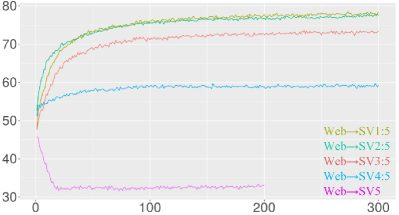
Figure S1: Validation accuracy over training epochs of our proposed domain adaptation framework with bridging domains. SV5 is used for validation set.

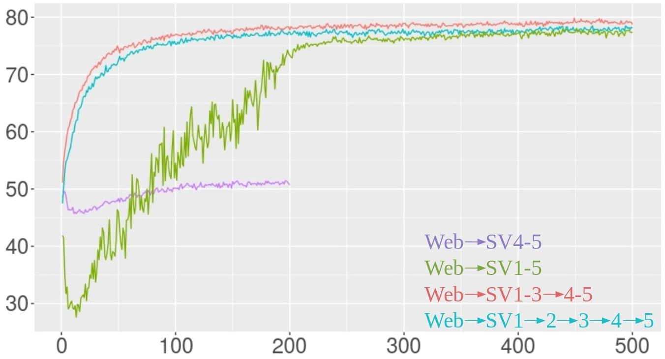
Figure S2: Performance on SV4–5 based on supervised bridging domain discovery using ground truth lighting conditions.

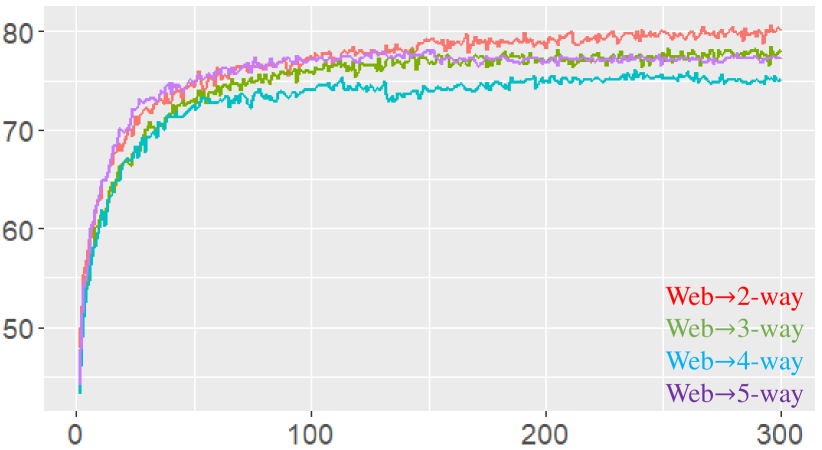
Figure S3: Performance on SV4–5 based on unsupervised bridging domain discovery using discriminator score of pretrained DANN.

S2.3 Unsupervised Discovery of Bridging Domains

While works on unsupervised discovery of latent domains exist [Gopalan et al.(2011)Gopalan, Li, and Chellappa, Gong et al.(2013)Gong, Grauman, and Sha, Gong et al.(2014)Gong, Grauman, and Sha], the choice of bridging domains remains a hard, unsolved problem. In this section, we present several approaches that we have exploited along this direction. Our initial approach is to quantify the closeness to the source domain of each image in the target domain by using the discriminator score $d_{\text{pre}}(f_{\text{pre}}(x))$ of pretrained DANN model as an indicator. This approach [Sohn et al.(2017)Sohn, Liu, Zhong, Yu, Yang, and Chandraker] intuitively makes sense as discriminator is trained to distinguish source and target domains, and those images from the target domain predicted as source domain are likely to be more similar to those images in the source domain, thus qualified as a bridging domain. Unfortunately, this is not necessarily true since the DANN is trained in an adversarial way and the discriminator at convergence should not be able to distinguish images from source and target domains [Goodfellow et al.(2014)Goodfellow, Pouget-Abadie, Mirza, Xu, Warde-Farley, Ozair, Courville, and Bengio]. Specifically, if we split the surveillance dataset into two domains based on the discriminator scores at each training epoch, and compute the AUC using the ground truth of day (SV1–3) and night (SV4–5) labels, we can see in Figure S7 that the AUC decreases as the number of training epochs increases. Meanwhile, as shown in Figure S6, S6 and S6, we visualize images from the surveillance domain based on the discriminator score from left-top the highest to right-bottom the lowest. With early stopping at the epoch 10, the discriminator of pretrained DANN model could be more discriminative in separating day and night images than those early stopped at epoch 50 and 150, which are closer to the convergence, thus cannot discriminate the images between the source and the target domains.

Based on our intuition and the visual inspection, we propose to construct bridging domains based on the discriminator score of the DANN model at epoch 10. By ranking the discriminator score $d_{\text{pre}}(f_{\text{pre}}(x))$ for $x\,{\in}\,\mathcal{D}_{T}$, we evenly split the unlabeled target data into $m$ sub-domains, denoted as $\mathcal{D}_{1},\cdots,\mathcal{D}_{m}$ for $m=2,\cdots,5$; $\mathcal{D}_{1}$ has the highest discriminator score and $\mathcal{D}_{m}$ the lowest. We then apply our proposed framework on $\mathcal{D}_{1},\cdots,\mathcal{D}_{m}$ with $\mathcal{D}_{m}$ as the target and the rest as the bridging domains. Results are shown in Figure S3 (also Table 5 from the main paper). Note that we use the SV4–5 for validation and testing so that the results are comparable with the reported ones in the main paper. The performance of our framework using unsupervised bridging domain discovery is highly competitive to those using ground truth lighting condition to construct bridging domains. Moreover, our proposed framework with discovered bridging domains demonstrates much more stable training curve (Figure S3) comparing to the baseline DANN model (Figure S3, Web$\rightarrow$SV1–5).

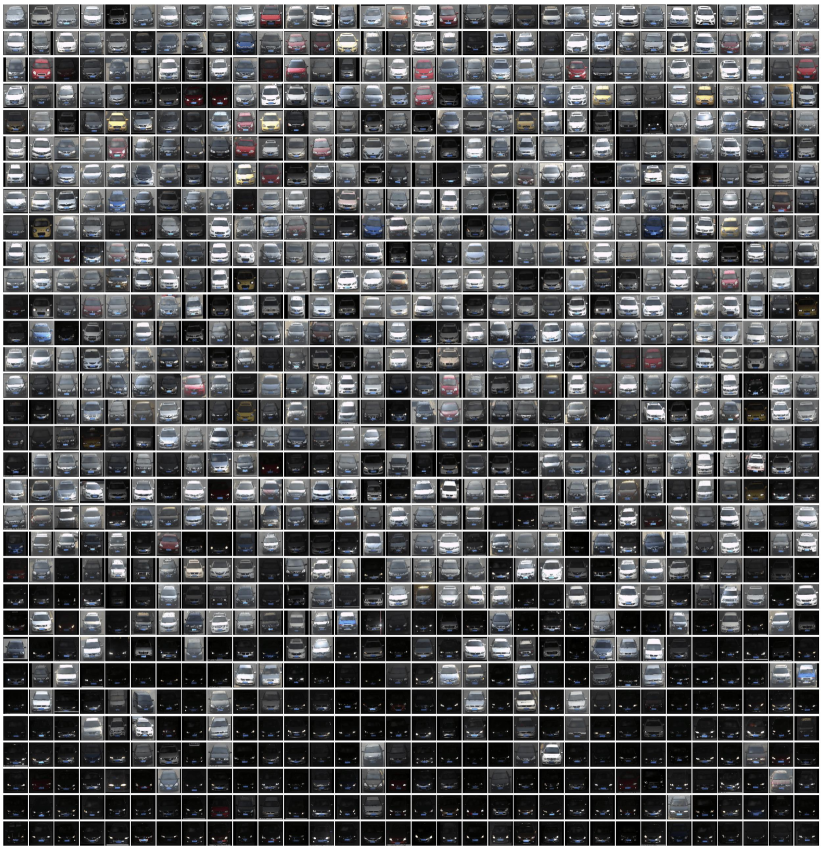
Figure S4: Early stopped at epoch 10.

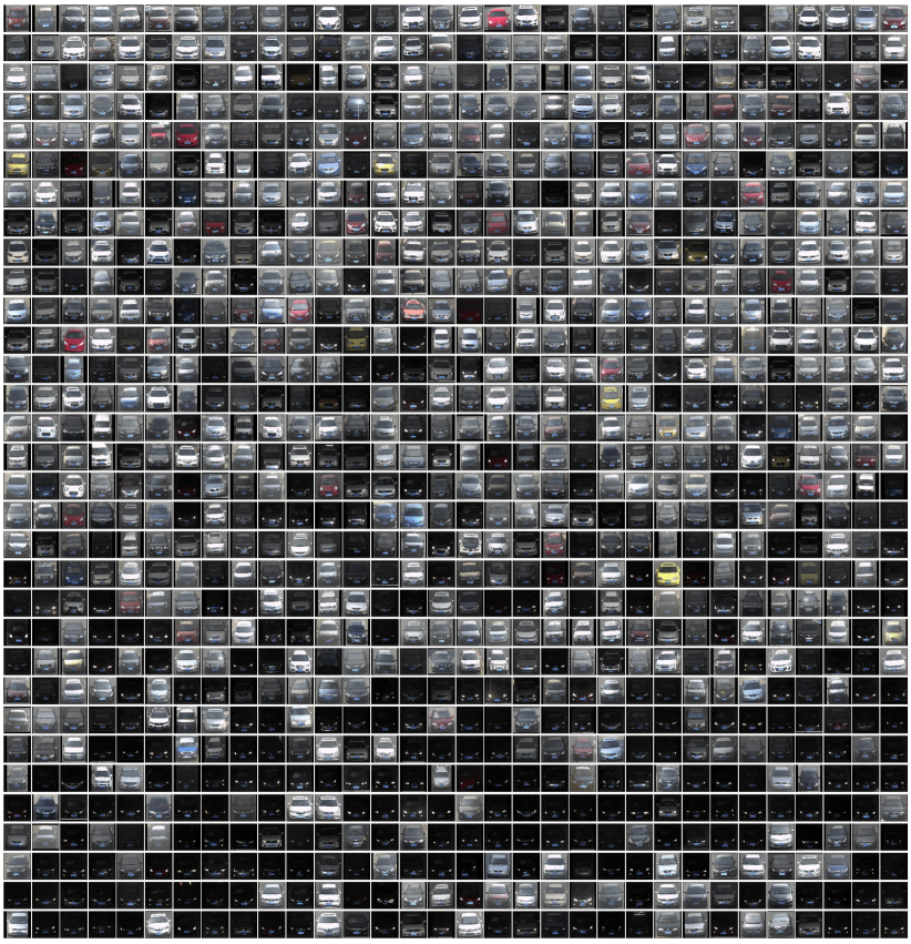
Figure S5: Early stopped at epoch 50.

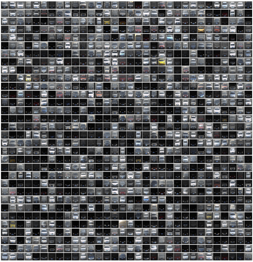
Figure S6: Early stopped at epoch 150.

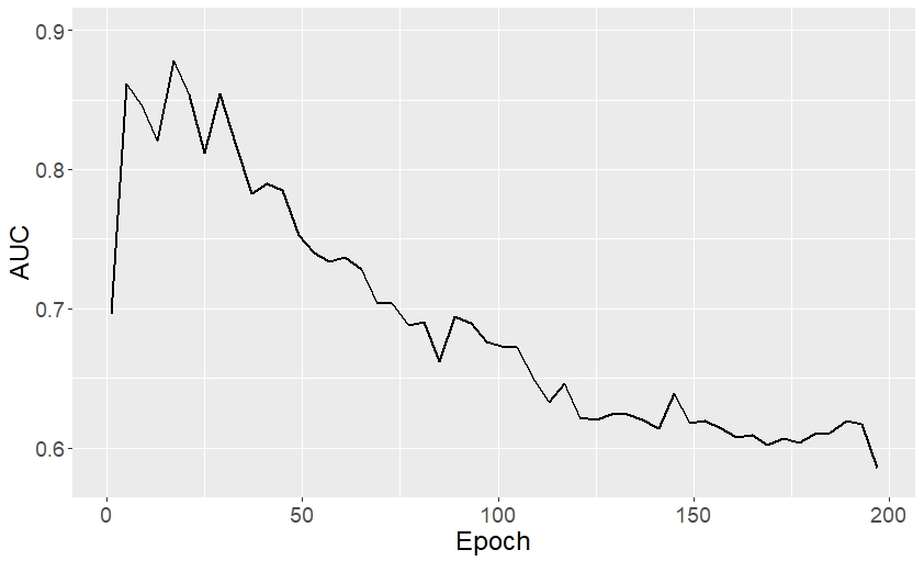
Figure S7: AUC between predicted closeness to the source domain using discriminator score and the ground-truth day/night labels at each training epoch.

In addition, we evaluate the performance of our proposed adaptation framework with discovered bridging domains using DANN models at epoch 50 and 150. Using Web$\to$2-way (78.62$\%$) as a reference, the results are 76.31$\%$ and 67.46$\%$ respectively. This confirms our observation in Figure S7 that our framework is the most effective when the bridging domains are retrieved by the discriminator of DANN stopped early.

While using discriminator scores demonstrates the effectiveness in unsupervised bridging domain detection, additional model selection stage (i.e., early stopping) is required to find a reliable discriminator $d_{\text{pre}}$. To avoid this, we can directly use different measure of closeness in the feature space between the source and the target domains. Specifically, we propose two measures, namely, the maximum mean discrepancy (MMD) [Gretton et al.(2012)Gretton, Borgwardt, Rasch, Schölkopf, and Smola] and the out-of-distribution (OOD) sample detection score [Hendrycks and Gimpel(2017)]. To evaluate these metrics, we first pretrain a classification model on the source domain only, with feature extractor $f_{\text{pre}}$ and classifier $C_{\text{pre}}$. Then, the pretrained extractor is applied to each of the target domain data $f_{\text{pre}}(x),x\in\mathcal{D}_{T}$. We compute the MMD between a target feature $f_{\text{pre}}(x^{(T)})$ and the entire source domain distribution $\{f_{\text{pre}}(x^{(S)})\}$ as follows:

$$\text{MMD}(f_{\text{pre}}(x^{(T)}),\{f_{\text{pre}}(x^{(S)})\})=\|\phi(f_{\text{pre}}(x^{(T)}))-\mathbb{E}_{x^{(S)}\sim\mathcal{D}_{S}}[\phi(f_{\text{pre}}(x^{(S)}))]\|_{\mathcal{H}},$$ (S23)

where $\phi:\mathcal{D}\rightarrow\mathcal{H}$ is the kernel mapping, and $\mathcal{H}$ is the a reproducing kernel Hilbert space (RKHS). By ranking the target domain based on the MMD values (the smaller the MMD, the closer the target feature is to the source domain), we can split target domain into several sub domains, where the ones that are close to the source domain can be considered as the bridging domains.

Alternatively, we can use the out-of-distribution (OOD) sample detection methods [Hendrycks and Gimpel(2017)]. Consider the output of the pretrained classifier for a target sample is $\hat{y}^{(T)}=C_{\text{pre}}(f_{\text{pre}}(x^{(T)}))$, such that $\hat{y}^{(T)}\sim\mathcal{Y}$ has $N$ categories, denoted as $\hat{y}^{(T)}=\{\hat{y}_{1}^{(T)},\cdots,\hat{y}_{N}^{(T)}\}$. Each $\hat{y}_{i}^{(T)}$ is the probability of $x^{(T)}$ being in category $i$. The OOD sample detection algorithm basically calculates:

$$\text{OOD}(\hat{y}^{(T)})=\max_{i}\sigma(\hat{y}_{i}^{(T)}),$$ (S24)

where $\sigma(\cdot)$ is the softmax function. The lower the value of $\text{OOD}(\hat{y}^{(T)})$ is, the more likely $x^{(T)}$ would be an out-of-distribution sample, and the further it is from the source domain. Similar to the MMD based approach, we can split the target domain based on the OOD score of every target domain sample.

As shown in Table 5 from the main paper, the discriminator score based approach achieves the highest AUC of $0.85$. Without any requirement of early stopping, the MMD based approach provides an AUC of $0.79$, and competitive model performance to the one from the discriminator score. The AUC from the OOD approach is relatively low at $0.69$, and the model performance is lower than the other two. Moreover, we observe that the classification accuracy is well correlated with the AUC score, suggesting the importance of more advanced algorithms [Liang et al.(2018)Liang, Li, and Srikant, Lee et al.(2018)Lee, Lee, Lee, and Shin] for measuring the closeness sensibly of the target example to the source domain.

References

- [Arbelaez et al.(2011)Arbelaez, Maire, Fowlkes, and Malik] Pablo Arbelaez, Michael Maire, Charless Fowlkes, and Jitendra Malik. Contour detection and hierarchical image segmentation. TPAMI, 2011.
- [Ben-David et al.(2007)Ben-David, Blitzer, Crammer, and Pereira] Shai Ben-David, John Blitzer, Koby Crammer, and Fernando Pereira. Analysis of representations for domain adaptation. In NIPS, 2007.
- [Ben-David et al.(2010)Ben-David, Blitzer, Crammer, Kulesza, Pereira, and Vaughan] Shai Ben-David, John Blitzer, Koby Crammer, Alex Kulesza, Fernando Pereira, and Jennifer Wortman Vaughan. A theory of learning from different domains. Machine learning, 2010.
- [Bengio et al.(2009)Bengio, Louradour, Collobert, and Weston] Yoshua Bengio, Jérôme Louradour, Ronan Collobert, and Jason Weston. Curriculum learning. In ICML, 2009.
- [Bousmalis et al.(2016)Bousmalis, Trigeorgis, Silberman, Krishnan, and Erhan] Konstantinos Bousmalis, George Trigeorgis, Nathan Silberman, Dilip Krishnan, and Dumitru Erhan. Domain separation networks. In NIPS, 2016.
- [Chen et al.(2018a)Chen, Papandreou, Kokkinos, Murphy, and Yuille] Liang-Chieh Chen, George Papandreou, Iasonas Kokkinos, Kevin Murphy, and Alan L Yuille. Deeplab: Semantic image segmentation with deep convolutional nets, atrous convolution, and fully connected crfs. TPAMI, 2018a.
- [Chen et al.(2018b)Chen, Li, Sakaridis, Dai, and Van Gool] Yuhua Chen, Wen Li, Christos Sakaridis, Dengxin Dai, and Luc Van Gool. Domain adaptive faster r-cnn for object detection in the wild. In CVPR, 2018b.
- [Cordts et al.(2016)Cordts, Omran, Ramos, Rehfeld, Enzweiler, Benenson, Franke, Roth, and Schiele] Marius Cordts, Mohamed Omran, Sebastian Ramos, Timo Rehfeld, Markus Enzweiler, Rodrigo Benenson, Uwe Franke, Stefan Roth, and Bernt Schiele. The cityscapes dataset for semantic urban scene understanding. In CVPR, 2016.
- [Courty et al.(2015)Courty, Flamary, Tuia, and Rakotomamonjy] Nicolas Courty, Rémi Flamary, Devis Tuia, and Alain Rakotomamonjy. Optimal transport for domain adaptation. TPAMI, 2015.
- [Deng et al.(2009)Deng, Dong, Socher, Li, Li, and Fei-Fei] Jia Deng, Wei Dong, Richard Socher, Li-Jia Li, Kai Li, and Li Fei-Fei. Imagenet: A large-scale hierarchical image database. In CVPR, 2009.
- [Duchi et al.(2011)Duchi, Hazan, and Singer] John Duchi, Elad Hazan, and Yoram Singer. Adaptive subgradient methods for online learning and stochastic optimization. Journal of Machine Learning Research, 2011.
- [Ganin et al.(2016)Ganin, Ustinova, Ajakan, Germain, Larochelle, Laviolette, Marchand, and Lempitsky] Yaroslav Ganin, Evgeniya Ustinova, Hana Ajakan, Pascal Germain, Hugo Larochelle, François Laviolette, Mario Marchand, and Victor Lempitsky. Domain-adversarial training of neural networks. Journal of Machine Learning Research, 2016.
- [Girshick et al.(2014)Girshick, Donahue, Darrell, and Malik] Ross Girshick, Jeff Donahue, Trevor Darrell, and Jitendra Malik. Rich feature hierarchies for accurate object detection and semantic segmentation. In CVPR, 2014.
- [Gong et al.(2013)Gong, Grauman, and Sha] Boqing Gong, Kristen Grauman, and Fei Sha. Reshaping visual datasets for domain adaptation. In NIPS, 2013.
- [Gong et al.(2014)Gong, Grauman, and Sha] Boqing Gong, Kristen Grauman, and Fei Sha. Learning kernels for unsupervised domain adaptation with applications to visual object recognition. In ICCV, 2014.
- [Goodfellow et al.(2014)Goodfellow, Pouget-Abadie, Mirza, Xu, Warde-Farley, Ozair, Courville, and Bengio] Ian Goodfellow, Jean Pouget-Abadie, Mehdi Mirza, Bing Xu, David Warde-Farley, Sherjil Ozair, Aaron Courville, and Yoshua Bengio. Generative adversarial nets. In NIPS, 2014.
- [Gopalan et al.(2011)Gopalan, Li, and Chellappa] Raghuraman Gopalan, Ruonan Li, and Rama Chellappa. Domain adaptation for object recognition: An unsupervised approach. In ICCV, 2011.
- [Gretton et al.(2012)Gretton, Borgwardt, Rasch, Schölkopf, and Smola] Arthur Gretton, Karsten M Borgwardt, Malte J Rasch, Bernhard Schölkopf, and Alexander Smola. A kernel two-sample test. Journal of Machine Learning Research, 13(Mar):723–773, 2012.
- [He et al.(2016)He, Zhang, Ren, and Sun] Kaiming He, Xiangyu Zhang, Shaoqing Ren, and Jian Sun. Deep residual learning for image recognition. In CVPR, 2016.
- [Hendrycks and Gimpel(2017)] Dan Hendrycks and Kevin Gimpel. A baseline for detecting misclassified and out-of-distribution examples in neural networks. In ICLR, 2017.
- [Hoffman et al.(2016)Hoffman, Wang, Yu, and Darrell] Judy Hoffman, Dequan Wang, Fisher Yu, and Trevor Darrell. Fcns in the wild: Pixel-level adversarial and constraint-based adaptation. arXiv preprint arXiv:1612.02649, 2016.
- [Hoffman et al.(2018)Hoffman, Tzeng, Park, Zhu, Isola, Saenko, Efros, and Darrell] Judy Hoffman, Eric Tzeng, Taesung Park, Jun-Yan Zhu, Phillip Isola, Kate Saenko, Alexei A Efros, and Trevor Darrell. Cycada: Cycle-consistent adversarial domain adaptation. In ICML, 2018.
- [Hu et al.(2018)Hu, Shen, and Sun] Jie Hu, Li Shen, and Gang Sun. Squeeze-and-excitation networks. In CVPR, June 2018.
- [Inoue et al.(2018)Inoue, Furuta, Yamasaki, and Aizawa] Naoto Inoue, Ryosuke Furuta, Toshihiko Yamasaki, and Kiyoharu Aizawa. Cross-domain weakly-supervised object detection through progressive domain adaptation. In CVPR, June 2018.
- [Ioffe and Szegedy(2015)] Sergey Ioffe and Christian Szegedy. Batch normalization: Accelerating deep network training by reducing internal covariate shift. ICML, 2015.
- [Kingma and Ba(2015)] Diederik Kingma and Jimmy Ba. Adam: A method for stochastic optimization. In ICLR, 2015.
- [Krizhevsky et al.(2012)Krizhevsky, Sutskever, and Hinton] Alex Krizhevsky, Ilya Sutskever, and Geoffrey E Hinton. Imagenet classification with deep convolutional neural networks. In NIPS, 2012.
- [LeCun et al.(1998)LeCun, Bottou, Bengio, and Haffner] Yann LeCun, Léon Bottou, Yoshua Bengio, and Patrick Haffner. Gradient-based learning applied to document recognition. Proceedings of the IEEE, 1998.
- [Lee et al.(2018)Lee, Lee, Lee, and Shin] Kimin Lee, Kibok Lee, Honglak Lee, and Jinwoo Shin. A simple unified framework for detecting out-of-distribution samples and adversarial attacks. In NIPS, 2018.
- [Liang et al.(2018)Liang, Li, and Srikant] Shiyu Liang, Yixuan Li, and R Srikant. Enhancing the reliability of out-of-distribution image detection in neural networks. In ICLR, 2018.
- [Mansour et al.(2009)Mansour, Mohri, and Rostamizadeh] Yishay Mansour, Mehryar Mohri, and Afshin Rostamizadeh. Domain adaptation with multiple sources. In NIPS, 2009.
- [Netzer et al.(2011)Netzer, Wang, Coates, Bissacco, Wu, and Ng] Yuval Netzer, Tao Wang, Adam Coates, Alessandro Bissacco, Bo Wu, and Andrew Y Ng. Reading digits in natural images with unsupervised feature learning. In NIPS Workshop, 2011.
- [Pan et al.(2010)Pan, Yang, et al.] Sinno Jialin Pan, Qiang Yang, et al. A survey on transfer learning. IEEE Transactions on knowledge and data engineering, 2010.
- [Paul et al.(2020)Paul, Tsai, Schulter, Roy-Chowdhury, and Chandraker] Sujoy Paul, Yi-Hsuan Tsai, Samuel Schulter, Amit K. Roy-Chowdhury, and Manmohan Chandraker. Domain adaptive semantic segmentation using weak labels. In European Conference on Computer Vision (ECCV), 2020.
- [Ren et al.(2015)Ren, He, Girshick, and Sun] Shaoqing Ren, Kaiming He, Ross Girshick, and Jian Sun. Faster R-CNN: Towards Real-Time Object Detection with Region Proposal Networks. In NIPS, 2015.
- [Richter et al.(2016)Richter, Vineet, Roth, and Koltun] Stephan R Richter, Vibhav Vineet, Stefan Roth, and Vladlen Koltun. Playing for data: Ground truth from computer games. In ECCV, 2016.
- [Sakaridis et al.(2018)Sakaridis, Dai, and Van Gool] Christos Sakaridis, Dengxin Dai, and Luc Van Gool. Semantic foggy scene understanding with synthetic data. IJCV, 2018.
- [Shelhamer et al.(2017)Shelhamer, Long, and Darrell] E. Shelhamer, J. Long, and T. Darrell. Fully convolutional networks for semantic segmentation. PAMI, 2017.
- [Simonyan and Zisserman(2015)] Karen Simonyan and Andrew Zisserman. Very deep convolutional networks for large-scale image recognition. In ICLR, 2015.
- [Sohn et al.(2017)Sohn, Liu, Zhong, Yu, Yang, and Chandraker] Kihyuk Sohn, Sifei Liu, Guangyu Zhong, Xiang Yu, Ming-Hsuan Yang, and Manmohan Chandraker. Unsupervised domain adaptation for face recognition in unlabeled videos. In ICCV, 2017.
- [Su et al.(2020)Su, Tsai, Sohn, Liu, Maji, and Chandraker] Jong-Chyi Su, Yi-Hsuan Tsai, Kihyuk Sohn, Buyu Liu, Subhransu Maji, and Manmohan Chandraker. Active adversarial domain adaptation. In WACV, 2020.
- [Szegedy et al.(2015)Szegedy, Liu, Jia, Sermanet, Reed, Anguelov, Erhan, Vanhoucke, and Rabinovich] Christian Szegedy, Wei Liu, Yangqing Jia, Pierre Sermanet, Scott Reed, Dragomir Anguelov, Dumitru Erhan, Vincent Vanhoucke, and Andrew Rabinovich. Going deeper with convolutions. In CVPR, 2015.
- [Tan et al.(2015)Tan, Song, Zhong, and Yang] Ben Tan, Yangqiu Song, Erheng Zhong, and Qiang Yang. Transitive transfer learning. In SIGKDD, 2015.
- [Tsai et al.(2018)Tsai, Hung, Schulter, Sohn, Yang, and Chandraker] Yi-Hsuan Tsai, Wei-Chih Hung, Samuel Schulter, Kihyuk Sohn, Ming-Hsuan Yang, and Manmohan Chandraker. Learning to adapt structured output space for semantic segmentation. In CVPR, June 2018.
- [Tsai et al.(2019)Tsai, Sohn, Schulter, and Chandraker] Yi-Hsuan Tsai, Kihyuk Sohn, Samuel Schulter, and Manmohan Chandraker. Domain adaptation for structured output via discriminative patch representations. In ICCV, 2019.
- [Tzeng et al.(2014)Tzeng, Hoffman, Zhang, Saenko, and Darrell] Eric Tzeng, Judy Hoffman, Ning Zhang, Kate Saenko, and Trevor Darrell. Deep domain confusion: Maximizing for domain invariance. arXiv preprint arXiv:1412.3474, 2014.
- [Tzeng et al.(2015)Tzeng, Hoffman, Darrell, and Saenko] Eric Tzeng, Judy Hoffman, Trevor Darrell, and Kate Saenko. Simultaneous deep transfer across domains and tasks. In ICCV, 2015.
- [Yang et al.(2015)Yang, Luo, Change Loy, and Tang] Linjie Yang, Ping Luo, Chen Change Loy, and Xiaoou Tang. A large-scale car dataset for fine-grained categorization and verification. In CVPR, 2015.
- [Zhao et al.(2018)Zhao, Zhang, Wu, Moura, Costeira, and Gordon] Han Zhao, Shanghang Zhang, Guanhang Wu, José MF Moura, Joao P Costeira, and Geoffrey J Gordon. Adversarial multiple source domain adaptation. In NIPS, 2018.