Weighted Irrigation Plans

Abstract

We model an irrigation network where lower branches must be thicker in order to support the weight of the higher ones. This leads to a countable family of ODEs, one for each branch, that must be solved by backward induction. Having introduced conditions that guarantee the existence and uniqueness of solutions, our main result establishes the lower semicontinuity of the corresponding cost functional, w.r.t. pointwise convergence of the irrigation plans. In turn, this yields the existence of an optimal irrigation plan, in the presence of these additional weights.

1 Introduction

In the classical irrigation problem with Gilbert cost [7], water is pumped out from a well and transported to finitely many locations $P_{1},\ldots,P_{n}$ by a network of pipes. The total cost is computed by

$$\sum~{}[\hbox{flux of water through the pipe}]^{\alpha}\times[\hbox{length of the pipe}].$$ (1.1)

Here the sum ranges over all pipes in the network, while $\alpha\in[0,1]$ is a fixed exponent.

This model is appropriate for an irrigation network built at ground level. On the other hand, sometimes one would like to model a network as a free standing structure. For example, in [3] the authors considered tree branches transporting water and nutrients from the root to all the leaves. In this case, one should take into account that the lower portion of each branch bears the weight of the upper part. As a result, the thickness (and hence cost per unit length) of the lower portion should be greater, even if the flux remains the same. This is indeed observed in nature, where the thickness of tree branches decreases in a continuous fashion, as one moves toward the tip.

Aim of this paper is to develop a general framework to describe this situation. As a first step, consider a single branch with length $\ell$, parameterized by arc-length $s\in[0,\ell]$, oriented from the root toward the tip. To account for the variable thickness of this branch we introduce a weight function $W=W(s)$. Assuming that the flux is constant along the entire branch, this will satisfy an ODE of the form

$$W^{\prime}(s)~{}=~{}-f(W(s)),$$ (1.2)

where $f$ is a non-negative, continuous function. A natural set of assumptions on $f$ is

• The function $f:\mathbb{R}_{+}\mapsto\mathbb{R}_{+}$ is continuous on $[0,\,+\infty[\,$, twice continuously differentiable for $s>0$, and satisfies

  $$f(0)=0,\qquad f^{\prime}(s)>0,\qquad f^{\prime\prime}(s)\leq 0\qquad\hbox{for all}~{}~{}s>0.$$ (1.3)

A typical example is $f(s)=cs^{\beta}$, for some $c\geq 0$ and $0<\beta\leq 1$.

1.1 A model with finitely many branches.

Next, we describe how to construct a family of weights $W_{i}(\cdot)$ in a network consisting of finitely many branches $\gamma_{i}$, $i=1,\ldots,N$. This will be achieved by induction, starting from the tip of each branch and proceeding backward toward the root.

To fix the ideas, let each branch $\gamma_{i}:[0,\ell_{i}]\mapsto\mathbb{R}^{d}$ be parameterized by arc-length, oriented from the root toward the tip. As shown in Fig. 1, call $P_{i}=\gamma_{i}(\ell_{i})$ the endpoint of the arc $\gamma_{i}$ and consider a measure $\mu$ consisting of finitely many point masses $m_{i}\geq 0$ located at points $P_{i}$. It is assumed that, for each node $P_{i}$, there is a unique path (i.e., a concatenation of arcs) connecting $P_{i}$ to the origin.

Call

$${\cal O}(i)~{}=~{}\Big{\{}j\in\{1,\ldots,N\}\,;~{}~{}\gamma_{j}(0)=P_{i}\Big{\}}$$ (1.4)

the set of branches originating from the node $P_{i}=\gamma_{i}(\ell_{i})$. Moreover, consider the sets of indices inductively defined by

$$\begin{array}[]{c}{\cal I}_{0}\,\doteq\,\emptyset,\qquad\qquad{\cal I}_{1}~{}\doteq~{}\Big{\{}i\in\{1,\ldots,N\}\,;~{}~{}{\cal O}(i)=\emptyset\Big{\}},\\[8.53581pt] {\cal I}_{p+1}~{}\doteq~{}\Big{\{}i\in\{1,\ldots,N\}\,;~{}~{}{\cal O}(i)\subseteq{\cal I}_{1}\cup\cdots\cup{\cal I}_{p}\Big{\}}\setminus({\cal I}_{1}\cup\cdots\cup{\cal I}_{p})\,.\end{array}$$ (1.5)

Roughly speaking, ${\cal I}_{1}$ is the set of outer-most branches. Branches in ${\cal I}_{p}$ originate from the tips of branches in ${\cal I}_{p+1}$, etc. Since the graph contains no loops, according to the above construction the set $\{1,\ldots,N\}$ is the disjoint union of the sets ${\cal I}_{p}$, $p\geq 1$.

For each branch $i\in\{1,\ldots,N\}$, a weight function $W_{i}(\cdot)$ can now be defined in terms of the following rules:

• The weight at the tip of the $i$-th branch is

  $$\overline{W}_{i}~{}\doteq~{}W_{i}(\ell_{i})~{}=~{}m_{i}+\sum_{j\in{\cal O}(i)}W_{j}(0+).$$ (1.6)

• Along each branch $\gamma_{i}$, the weight $W_{i}(\cdot)$ is absolutely continuous and satisfies the ODE

  $$W^{\prime}_{i}(s)~{}=~{}-f(W_{i}(s))\qquad\qquad s\in\,]0,\ell_{i}]\,.$$ (1.7)

According to (i)-(ii), the solution can be computed by induction on the entire tree, first on all branches $i\in{\cal I}_{1}$, then on all branches $i\in{\cal I}_{2}$, etc. For sake of definiteness, we assume

$$m_{i}\,>\,0\qquad\hbox{for all}~{}i\in{\cal I}_{1}\,.$$ (1.8)

This guarantees that the flux along every branch is strictly positive. In turn, by (1.3), it implies that the backward Cauchy problem (1.6)-(1.7) on $[0,\ell_{i}]$ has a unique solution. Example 1. When $f(s)=cs^{\beta}$, the Cauchy problem (1.6)-(1.7) can be solved explicitly. Namely:

$$\overline{W}_{i}^{1-\beta}-W_{i}^{1-\beta}(s)~{}=~{}c(1-\beta)(s-\ell_{i}),$$

$$W_{i}(s)~{}=~{}\Big{(}\overline{W}_{i}^{1-\beta}+c(1-\beta)(\ell_{i}-s)\Big{)}^{1\over 1-\beta}.$$ (1.9)

In particular, from (1.6) we deduce the inductive rule

$$\overline{W}_{i}~{}=~{}m_{i}+\sum_{j\in{\cal O}(i)}\Big{(}\overline{W}_{j}^{1-\beta}+c(1-\beta)\ell_{j}\Big{)}^{1\over 1-\beta}.$$ (1.10)

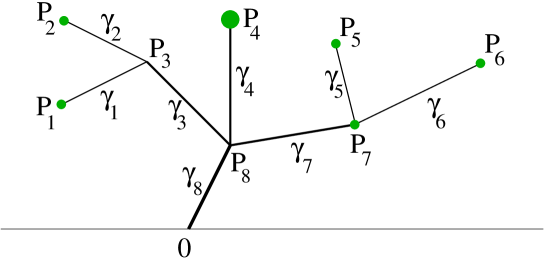
Figure 1: According to (1.5), the branches of this tree are partitioned according to ${\cal I}_{1}=\{1,2,4,5,6\}$, ${\cal I}_{2}=\{3,7\}$, ${\cal I}_{3}=\{8\}$. Weights can be constructed by induction, solving the backward Cauchy problems (1.6)-(1.7) first along the arcs $\gamma_{i}$, $i\in{\cal I}_{1}$, then for $i\in{\cal I}_{2}$, etc.

In the presence of a weight function $W$, for a given $\alpha\in\,]0,1]$ the total weighted cost of the irrigation network is then defined as

$$E^{W,\alpha}~{}\doteq~{}\sum_{i}\int_{0}^{\ell_{i}}[W_{i}(s)]^{\alpha}\,ds.$$ (1.11)

More generally, given a positive, nondecreasing, concave function $\psi:\mathbb{R}_{+}\mapsto\mathbb{R}_{+}$, satisfying the same assumptions as $f$ in (A1). We then define

$$E^{W,\psi}~{}\doteq~{}\sum_{i}\int_{0}^{\ell_{i}}\psi\bigl{(}W_{i}(s)\bigr{)}\,ds.$$ (1.12)

Remark 1.1

In the case where $f\equiv 0$, the weight functions are constant along every branch:

$$W_{i}(s)~{}=~{}\hbox{flux through}~{}\gamma_{i}\,,\qquad\qquad s\in[0,\ell_{i}]\,.$$

Hence the total weighted cost (1.11) coincides with the Gilbert cost (1.1).

Remark 1.2

In the special case where $\beta=\alpha$, so that $f(s)=cs^{\alpha}$, in view of (1.9) this cost is computed by

$$E^{W,\alpha}~{}\doteq~{}\sum_{i}\int_{0}^{\ell_{i}}\Big{(}\overline{W}_{i}^{1-\alpha}+c(1-\alpha)(\ell_{i}-s)\Big{)}^{\alpha\over 1-\alpha}\,ds.$$ (1.13)

When $\alpha=1-\alpha=1/2$, the formulas (1.10) and (1.13) further simplify to

$$\overline{W}_{i}~{}=~{}m_{i}+\sum_{j\in{\cal O}(i)}\Big{(}\overline{W}_{j}^{1/2}+{c\ell_{j}\over 2}\Big{)}^{2},\qquad\quad E^{W,\alpha}~{}\doteq~{}\sum_{i}\Big{(}\ell_{i}\overline{W}_{i}^{1/2}+{c\ell_{i}^{2}\over 4}\Big{)}.$$

Aim of the present paper is to extend the theory of optimal irrigation networks [1, 2, 3, 10, 20, 21], accounting for the presence of weights in the cost function. In essence, this requires the solution of a countable family of measure-valued ODEs, one for each branch of the network.

In the case of a finite network, where $\mu$ consists of finitely many atoms, our definition reduces to (1.11). For a general network, irrigating a positive Radon measure $\mu$, the weighted cost will be defined as a limit of an increasing sequence of approximations. For any $\varepsilon>0$, these approximations are obtained by restricting the transport plan to a finite set of paths where the flux is $\geq\varepsilon$.

Besides showing how this family of weights can be uniquely determined, our main results include the lower semicontinuity of the weighted irrigation cost. As an immediate consequence, this yields the existence of optimal weighted irrigation plans. Furthermore, the optimization problems for tree branches considered in [4, 5] still have solutions when the cost functional includes the presence of weights.

The remainder of the paper is organized as follows. Section 2 reviews some basic definitions and results concerning the Lagrangian approach to optimal irrigation plans. For later use, we also include some lemmas on ODEs with measure-valued right hand side, formulated as integral equations. In Section 3 we provide a detailed construction of the weight functions, and the total weighted cost of an irrigation plan. The lower semicontinuity of the weighted cost, w.r.t. pointwise convergence of the particle paths, is stated as Theorem 4.1, and proved in Section 4. In Section 5 we consider a more general model where the increase in the thickness of a branch, as one moves from the tip toward the root, depends also on the inclination of the branch itself. The ODE (1.2) is thus replaced by

$$W^{\prime}(s)~{}=~{}-f(\dot{\gamma}(s),W(s)),$$ (1.14)

assuming that $f$ is continuous in both variables, and that the map $v\mapsto f(v,W)$ is positively homogeneous and convex w.r.t. the variable $v\in\mathbb{R}^{d}$. We show that all previous results, including the lower semicontinuity of the weighted irrigation cost, remain valid in this more general case.

Finally, in Section 6 we prove the existence of an optimal weighted irrigation plan for a given measure $\mu$, and the lower semicontinuity of the weighted irrigation cost w.r.t. weak convergence of measures: $\mu_{n}\rightharpoonup\mu$. In particular, the existence of solutions to the optimization problems for tree branches studied in [4, 5] remains valid also in the presence of weights.

The problem of determining which measures have a finite or infinite weighted irrigation cost, depending on the dimension of their support, will be discussed in the forthcoming paper [19]. An interesting open question is whether, in the presence of weights, an optimal irrigation plan can be computed using a suitable Modica-Mortola approximation based on $\Gamma$-convergence, as in [12, 13, 14, 17].

A general introduction to the theory of ramified transport can be found in [1]. For solutions of ODEs with measure-valued right hand side we refer to [6, 15].

2 Preliminaries

We recall some basic definitions from [1]. Throughout the following, we say that a map $\gamma(\cdot)$ is 1-Lipschitz if it is Lipschitz continuous with Lipschitz constant 1. We denote by $\Gamma$ the set of all 1-Lipschitz maps $\gamma:\mathbb{R}_{+}\mapsto\mathbb{R}^{d}$. By Ascoli-Arzela’s theorem (see Lemma 3.4 in [1]), this is a compact metric space with the distance

$$d(\gamma_{1},\gamma_{2})~{}\doteq~{}\sup_{k>1}~{}{1\over k}\,\Big{\{}\max_{s\in[0,k]}|\gamma_{1}(s)-\gamma_{2}(s)|\Big{\}}.$$ (2.1)

Notice that (2.1) corresponds to the topology of uniform convergence on compact sets.

Definition 2.1

Let $\mu$ be a positive Radon measure on $\mathbb{R}^{d}$, with total mass $M\doteq\mu(\mathbb{R}^{d})$. An irrigation plan for $\mu$ is a function

$$\chi:[0,M]\times\mathbb{R}_{+}\mapsto\mathbb{R}^{d},$$

measurable w.r.t. $\xi$ and continuous w.r.t. $t$, with the following properties.

• (regularity) For a.e. $\xi\in[0,M]$ the map $t\mapsto\chi(\xi,t)$ is 1-Lipschitz and eventually constant. Namely, there exists $\tau(\xi)\geq 0$ such that

  $$\left\{\begin{array}[]{cl}|\chi(\xi,t)-\chi(\xi,t^{\prime})|~{}\leq~{}|t-t^{\prime}|&\hbox{for all}~{}t,t^{\prime}\geq 0,\\[8.53581pt] \chi(\xi,t)~{}=~{}\chi(\xi,\tau(\xi))&\hbox{for every}~{}t\geq\tau(\xi).\end{array}\right.$$

  Throughout the following, we denote by $\tau(\xi)$ is the smallest time $\tau$ such that $\chi(\xi,\cdot)$ is constant for $t\geq\tau$.

• ($\chi$ irrigates the measure $\mu$) For all $\xi\in[0,M]$ one has $\chi(\xi,0)=0$. Moreover, the push-forward of the Lebesgue measure on $[0,M]$ by the map $\xi\mapsto\chi(\xi,\tau(\xi))$ coincides with $\mu$. In other words, for every Borel set $V\subseteq\mathbb{R}^{d}$ on has

  $$\mu(V)~{}=~{}\hbox{meas}\Big{\{}\xi\in[0,M]\,;~{}~{}\chi(\xi,\tau(\xi))\in V\Big{\}}.$$ (2.2)

Remark 2.2

Relying on a theorem of Scorza-Dragoni [9, 18], one can construct a partition of the interval $[0,M]$ into countably many disjoint subsets

$$[0,M]~{}=~{}\left(\bigcup_{j=1}^{\infty}K_{j}\right)\cup{\cal N},$$ (2.3)

such that

• each $K_{j}$ is compact,

• the set ${\cal N}$ has measure zero,

• the restriction of $\chi$ to each product set $K_{j}\times\mathbb{R}_{+}$ is continuous.

Thanks to the above construction, measurability issues can be more easily resolved. For example, we have

Lemma 2.3

Let $K\subseteq[0,M]$ be a compact subset such that $\chi$ is continuous restricted to $K\times\mathbb{R}_{+}$. Then the map $\xi\mapsto\tau(\xi)$ is lower semicontinuous restricted to $K$.

Proof. Indeed, consider a sequence $\xi_{n}\to\xi$ of points in $K$. If $\liminf\tau(\xi_{n})=+\infty$ there is nothing to prove. Otherwise, by taking a subsequence, we can assume

$$\lim_{n\to\infty}\tau(\xi_{n})~{}=~{}\bar{\tau}.$$

By assumption, the continuous functions $\chi(\xi_{n},\cdot)$ converge to $\chi(\xi,\cdot)$ uniformly on compact sets. For any $\varepsilon>0$, all but finitely many of these functions are constant on $[\bar{\tau}+\varepsilon,\,+\infty[\,$. Hence also $\chi(\xi,\cdot)$ is constant on this same domain. Since $\varepsilon>0$ is arbitrary, we conclude that $\chi(\xi,\cdot)$ is constant on $[\bar{\tau},+\infty[\,$. Hence $\tau(\xi)\leq\bar{\tau}$, as claimed. MM     

Corollary 2.4

Given any $\varepsilon>0$ there exists a compact set $K\subseteq[0,M]$, with

$$\hbox{meas}\Big{(}[0,M]\setminus K\Big{)}~{}<~{}\varepsilon,$$ (2.4)

and such that

• the map $\xi\mapsto\chi(\xi,\cdot)$ is continuous restricted to $K$,

• the map $\xi\mapsto\tau(\xi)$ is continuous restricted to $K$.

Proof. By Remark 2.2, we can choose $K=\cup_{j=1}^{\nu}K_{j}$ with $\nu$ large enough so that (2.4) holds. Since $\chi$ is continuous on each $K_{j}$, the statement (i) follows immediately. By Lemma 2.3 the map $\xi\mapsto\tau(\xi)$ is measurable on $K$. By Lusin’s theorem, there exists a smaller compact set $K_{0}\subseteq K$, still with meas$([0,M]\setminus K_{0})~{}<~{}\varepsilon$, such that the restriction of $\tau(\cdot)$ to $K_{0}$ is continuous. By replacing $K$ with $K_{0}$, the conclusion (ii) of the Corollary is satisfied. MM     

The usual definition of irrigation cost involves the multiplicity of a point $x=\chi(\xi,t)$, defined as

$$|x|_{\chi}~{}\doteq~{}\hbox{meas}\Big{(}\{\xi\in[0,M]\,;~{}~{}\chi(\xi,t)=x~{}~{}\hbox{for some}~{}t\geq 0\}\Big{)}.$$ (2.5)

In the present case, this must be replaced by a different concept, related to the single-path property.

Definition 2.5

We say that two 1-Lipschitz maps $\gamma:[0,t]\mapsto\mathbb{R}^{d}$ and $\gamma^{\prime}:[0,t^{\prime}]\mapsto\mathbb{R}^{d}$ are equivalent if they are parameterizations of the same curve. That is, if there exists an interval $[0,T]$ and nondecreasing, Lipschitz continuous surjective maps $s\mapsto\eta(s)$ and $s\mapsto\eta^{\prime}(s)$ from $[0,T]$ onto $[0,t]$ and $[0,t^{\prime}]$ respectively, such that

$$\gamma(\eta(s))~{}=~{}\gamma^{\prime}(\eta^{\prime}(s))\qquad\qquad\hbox{for all}~{}s\in[0,T].$$ (2.6)

If this is the case, we write $\gamma\simeq\gamma^{\prime}$.

Remark 2.6

Given a 1-Lipschitz map $\gamma:[0,t]\mapsto\mathbb{R}^{d}$, its arc-length re-parameterization is the map

$$\sigma~{}\mapsto~{}\gamma(s(\sigma))$$

where, for every $\sigma$, one has

$$\int_{0}^{s(\sigma)}|\dot{\gamma}(\zeta)|\,d\zeta~{}=~{}\sigma.$$

According to the above definition, two maps $\gamma:[0,t]\mapsto\mathbb{R}^{d}$ and $\gamma^{\prime}:[0,t^{\prime}]\mapsto\mathbb{R}^{d}$ are equivalent if and only if their arc-length re-parameterizations coincide.

Remark 2.7

In Definition 2.5, one can always take $T=t+t^{\prime}$ and assume that both functions $\eta,\eta^{\prime}$ are 1-Lipschitz. Indeed, let $\eta,\eta^{\prime}$ be maps from $[0,T]$ onto $[0,t]$ and $[0,t^{\prime}]$ respectively, such that (2.6) holds.

For $s\in[0,T]$, define the nondecreasing, surjective map $\sigma:[0,T]\mapsto[0,\widetilde{T}]\doteq[0,t+t^{\prime}]$ by setting

$$\sigma(s)~{}\doteq~{}\eta(s)+\eta^{\prime}(s).$$

We then define the maps $\tilde{\eta},\tilde{\eta}^{\prime}$ from $[0,\widetilde{T}]$ into $[0,t]$ and $[0,t^{\prime}]$ implicitly, by setting

$$\tilde{\eta}(\sigma(s))~{}\doteq~{}\eta(s),\qquad\quad\tilde{\eta}^{\prime}(\sigma(s))~{}\doteq~{}\eta^{\prime}(s)\qquad s\in[0,T].$$ (2.7)

We claim that $\tilde{\eta}$ and $\tilde{\eta}^{\prime}$ are 1-Lipschitz. Indeed, let $\sigma_{1}=\sigma(s_{1})<\sigma(s_{2})=\sigma_{2}$. Then

$$\bigl{[}\tilde{\eta}(\sigma_{2})-\tilde{\eta}(\sigma_{1})\bigr{]}+[\tilde{\eta}(\sigma_{2})-\tilde{\eta}(\sigma_{1})]~{}=~{}[\eta(s_{2})+\eta^{\prime}(s_{2})]-[\eta(s_{1})+\eta^{\prime}(s_{1})]~{}=~{}\sigma_{2}-\sigma_{1}\,.$$

The identity $\gamma(\tilde{\eta}(s))~{}=~{}\gamma^{\prime}(\tilde{\eta}^{\prime}(s))$ now follows from (2.6) and (2.7).

Throughout the following, we denote by $\gamma\Big{|}_{[0,t]}$ the restriction of a map $\gamma$ to the interval $[0,t]$.

Definition 2.8

Let $\chi:[0,M]\times\mathbb{R}_{+}\mapsto\mathbb{R}^{d}$ be an irrigation plan for the measure $\mu$. We define an equivalence relation on the set $[0,M]\times\mathbb{R}_{+}$ by setting $(\xi,t)\,\sim\,(\xi^{\prime},t^{\prime})$ whenever $\chi(\xi,\cdot)\Big{|}_{[0,t]}\simeq\chi(\xi^{\prime},\cdot)\Big{|}_{[0,t^{\prime}]}$. This means that the maps

$$s~{}\mapsto~{}\chi(\xi,s),\quad s\in[0,t]\qquad\hbox{and}\qquad s~{}\mapsto~{}\chi(\xi^{\prime},s),\quad s\in[0,t^{\prime}]$$

are equivalent in the sense of Definition 2.5.

The multiplicity of $(\xi,t)$ is then defined as

$$m(\xi,t)~{}\doteq~{}\hbox{meas}\Big{(}\bigl{\{}\xi^{\prime}\in[0,M]\,;~{}~{}(\xi^{\prime},t^{\prime})\sim(\xi,t)~{}~{}\hbox{for some}~{}t^{\prime}>0\bigr{\}}\Big{)}.$$ (2.8)

Remark 2.9

The multiplicity $m(\xi,t)$ measures the total amount of particles that pass through the point $x=\chi(\xi,t)$ traveling along exactly the same path as the particle $\xi$. If $\chi$ has the single path property (see Chapter 7 in [1]), then $m(\xi,t)=|\chi(\xi,t)|_{\chi}$. However, for a general irrigation plan we only have the inequality

$$m(\xi,t)~{}\leq~{}|\chi(\xi,t)|_{\chi}\,.$$ (2.9)

Notice that one may well have

$$\chi(\xi,t)\,=\,\chi(\xi^{\prime},t^{\prime})\qquad\hbox{but}\qquad m(\xi,t)\,\not=\,m(\xi^{\prime},t^{\prime}).$$

Given an irrigation plan $\chi:[0,M]\times\mathbb{R}_{+}\mapsto\mathbb{R}^{d}$, throughout the following we shall use a basic assumption, which is needed in order that the total cost be finite. As in part (i) of Definition 2.1, we denote by $\tau(\xi)$ the time when the particle $\xi$ reaches its final destination.

• For a.e. $\xi\in[0,M]$, one has $m(\xi,t)>0$ for every $0\leq t<\tau(\xi)$.

In other words, for any particle $\xi$ and any $t\in[0,\,\tau(\xi)[\,$, there is a positive amount of other particles that travel along the same path $\chi(\xi,\cdot)\Big{|}_{[0,t]}$.

The next two lemmas establish various properties of the multiplicity function introduced in Definition 2.8

Lemma 2.10

For any $\varepsilon>0$ there exists a compact set $K\subseteq[0,M]$ satisfying (2.4), such that the set-valued function

$$F(\xi,t)~{}\doteq~{}\{\xi^{\prime}\in K\,;~{}~{}(\xi^{\prime},t^{\prime})\sim(\xi,t)~{}~{}\hbox{for some}~{}~{}t^{\prime}\geq 0\}$$ (2.10)

is upper semicontinuous on $K\times\mathbb{R}_{+}$.

Proof. 1. Given $\varepsilon>0$, let $K\subseteq[0,M]$ be the compact set constructed in Corollary 2.4. We claim that the graph of $F$, restricted to $K\times\mathbb{R}_{+}$, is closed. In other words, assume that

$$\xi_{n}\to\xi\,\qquad t_{n}\to t,\qquad\xi^{\prime}_{n}\to\xi^{\prime}\qquad\hbox{as}\quad n\to\infty,$$

and moreover

$$(\xi^{\prime}_{n},t^{\prime}_{n})\sim(\xi_{n},t_{n})\qquad\hbox{for all}~{}n\geq 1.$$

We need to show that there exists $t^{\prime}\geq 0$ such that $(\xi,t)\sim(\xi^{\prime},t^{\prime})$. 2. By the assumptions, according to Remark 2.7 for every $n\geq 1$ there exists an interval $[0,T_{n}]=[0,t_{n}+t^{\prime}_{n}]$ and two nondecreasing, 1-Lipschitz, surjective maps

$$\eta_{n}:[0,T_{n}]\,\mapsto[0,t_{n}],\qquad\eta^{\prime}_{n}:[0,T_{n}]\,\mapsto[0,t^{\prime}_{n}],$$

such that

$$\chi(\xi_{n},\eta_{n}(s))~{}=~{}\chi(\xi^{\prime}_{n},\eta^{\prime}_{n}(s))\qquad\hbox{for all}~{}s\in[0,T_{n}].$$ (2.11)

3. We now observe that, since the map $\xi\mapsto\tau(\xi)$ is continuous on the compact set $K$, it is uniformly bounded. We can thus assume that the sequence $(t^{\prime}_{n})_{n\geq 1}$ is bounded. Since $t_{n}\to t<+\infty$ and $T_{n}=t_{n}+t_{n}^{\prime}$, we have the uniform boundedness of $(T_{n})_{n\geq 1}$. By extracting a subsequence, one can assume

$$\lim_{n\to+\infty}t_{n}^{\prime}~{}=~{}t^{\prime},\qquad\lim_{n\to+\infty}T_{n}~{}=~{}T\,.$$ (2.12)

If $T_{n}<T$, we extend the maps $\eta_{n}$ and $\eta_{n}^{\prime}$ to the interval $[0,T]$ by setting $\eta_{n}(s)\doteq\eta_{n}(T_{n})$, $\eta_{n}^{\prime}(s)\doteq\eta_{n}^{\prime}(T_{n})$, for all $s\in(T_{n},T]$. Using the Ascoli-Arzelà theorem, by possibly extracting a subsequence we achieve the uniform convergence

$$\eta_{n}(\cdot)\to\eta(\cdot),\qquad\eta_{n}^{\prime}(\cdot)\to\eta^{\prime}(\cdot)\,,\qquad\hbox{ uniformly on }~{}[0,T]\,.$$ (2.13)

Here $\eta$ and $\eta^{\prime}$ are two nondecreasing, 1-Lipschitz, surjective maps from $[0,T]$ onto $[0,t]$ and $[0,t^{\prime}]$ respectively. By the continuity of $\chi(\cdot,\cdot)$ on $K\times\mathbb{R}_{+}$, from (2.11) we obtain

$$\chi(\xi,\eta(s))~{}=~{}\lim_{n\to\infty}\chi(\xi_{n},\eta_{n}(s))~{}=~{}\lim_{n\to\infty}\chi(\xi_{n}^{\prime},\eta_{n}^{\prime}(s))~{}=~{}\chi(\xi^{\prime},\eta^{\prime}(s))\qquad\hbox{ for all }s\in[0,T].$$ (2.14)

Therefore, $(\xi^{\prime},t^{\prime})\sim(\xi,t)$. MM     

Lemma 2.11

Let $\chi:[0,M]\times\mathbb{R}_{+}\mapsto\mathbb{R}^{d}$ be an irrigation plan for the measure $\mu$. Then the following holds.

• The map $(\xi,t)\mapsto m(\xi,t)$ is measurable.

• For each $\xi\in[0,M]$, the map $t\mapsto m(\xi,t)$ is non-increasing and left continuous.

• For any fixed $\varepsilon>0$, the stopping time

  $$\tau_{\varepsilon}(\xi)~{}\doteq~{}\max\,\Big{\{}t\in[0,\tau(\xi)]\,;~{}~{}m(\xi,t)\geq\varepsilon\Big{\}}$$ (2.15)

  is a measurable function of $\xi\in[0,M]$.

Proof. 1. Given $\varepsilon>0$, let $K\subseteq[0,M]$ be a compact set satisfying the conditions in Lemma 2.10. In terms of the multifunction $(\xi,t)\mapsto F(\xi,t)\subseteq K$ defined at (2.10), this implies the scalar function

$$(\xi,t)~{}\mapsto~{}\hbox{meas}(F(\xi,t))$$ (2.16)

is upper semicontinuous restricted to $K\times\mathbb{R}_{+}\,$. For $(\xi,t)\in K\times\mathbb{R}_{+}$ this implies

$$m(\xi,t)-\varepsilon~{}\leq~{}\hbox{meas}(F(\xi,t))~{}\leq~{}m(\xi,t).$$ (2.17)

2. Repeating the above construction for decreasing values of $\varepsilon$, we can find an increasing sequence of compact sets $(K_{n})_{n\geq 1}$, with $\hbox{meas}([0,M]\setminus K_{n})<1/n$, such that

$$m(\xi,t)-{1\over n}~{}\leq~{}\hbox{meas}(F_{n}(\xi,t))~{}\leq~{}m(\xi,t)\,.$$ (2.18)

Here $F_{n}$ is the multifunction defined at (2.10), with $K$ replaced by $K_{n}$. Notice that the function $(\xi,t)~{}\mapsto~{}\hbox{meas}(F_{n}(\xi,t))$ is upper semicontinuous restricted to $K_{n}\times\mathbb{R}_{+}$. Setting

$$m_{n}(\xi,t)~{}\doteq~{}\left\{\begin{array}[]{cl}\hbox{meas}(F_{n}(\xi,t))&\qquad\hbox{if}~{}~{}\xi\in K_{n}\,,\\[8.53581pt] 0&\qquad\hbox{if}~{}~{}\xi\notin K_{n}\,,\end{array}\right.$$

by (2.18) we have the pointwise convergence $m_{n}(\xi,t)\to m(\xi,t)$ for a.e. $\xi\in[0,M]$. Since each $m_{n}$ is measurable, the same holds for $m$. This proves (i). 3. By the definition of the multiplicity function in (2.8), it immediately follows that the map $t\mapsto m(\xi,t)$ is non-increasing. To prove its left continuity, fix $(\xi,t)\in[0,M]\times\mathbb{R}_{+}$ and consider an increasing sequence $t_{n}\uparrow t$. By monotonicity, it follows

$$\lim_{n\to\infty}m(\xi,t_{n})~{}=~{}\inf_{n}\,m(\xi,t_{n})~{}\geq~{}m(\xi,t)\,.$$ (2.19)

To prove that equality actually holds in (2.19), given any $\varepsilon>0$, let $K\subseteq[0,M]$ be a compact set satisfying the conditions in Lemma 2.10. By the upper semicontinuity of the multifunction $t\mapsto F(\xi,t)$ one has

$$m(\xi,t)~{}\geq~{}\hbox{meas}(F(\xi,t))~{}\geq~{}\limsup_{n\to\infty}~{}\hbox{meas}(F(\xi,t_{n}))~{}\geq~{}\limsup_{n\to\infty}~{}m(\xi,t_{n})-\varepsilon\,.$$ (2.20)

Since $\varepsilon>0$ was arbitrary, this proves statement (ii) of the lemma. 4. To prove (iii), we first observe that, by the arguments in the previous steps 1 - 2, for each fixed $t>0$ the map $\xi\mapsto m(\xi,t)$ is measurable. Moreover, by Corollary 2.4 it follows that $\xi\mapsto\tau(\xi)$ is measurable. For every $t>0$ we have the identity

$$\Big{\{}\xi\in[0,M]\,;~{}\tau_{\varepsilon}(\xi)\geq t\Big{\}}~{}=~{}\Big{\{}\xi\in[0,M]\,;~{}m(\xi,t)\geq\varepsilon\Big{\}}\bigcap\Big{\{}\xi\in[0,M]\,;~{}\tau(\xi)\geq t\Big{\}}.$$ (2.21)

This implies that the map $\tau_{\varepsilon}(\cdot)$ is measurable. MM     

2.1 ODE’s with measure-valued right hand side.

For future use, we now prove some results on existence and continuous dependence, for Carathéodory solutions to an ODE backward in time. Since in our equations the right hand side can possibly be a measure, it will be convenient to study directly the corresponding integral equations.

Lemma 2.12

Let $f:[\varepsilon,+\infty[\,\mapsto\mathbb{R}_{+}$ be Lipschitz continuous. For $t\in[0,T]$, let $t\mapsto m(t)$ be a non-increasing function with $m(T)\geq\varepsilon$.

• There exists a unique function $w:[0,T]\mapsto[\varepsilon,+\infty[\,$ which satisfies the integral equation

  $$w(t)~{}=~{}\int_{t}^{T}f(w(s))\,ds+m(t)\qquad\qquad\hbox{for all}~{}t\in[0,T].$$ (2.22)

• If $m_{1}(t)\leq m_{2}(t)$ for all $t\in[0,T]$, then the corresponding solutions of (2.22) satisfy

  $$w_{1}(t)~{}\leq~{}w_{2}(t)\qquad\qquad\hbox{for all}~{}t\in[0,T].$$ (2.23)

• Consider a sequence of measurable sets $J_{n}\subseteq[0,T]$ such that $\lim_{n\to\infty}\hbox{meas}(J_{n})=0$, and define the functions

  $$f_{n}(t,\omega)~{}\doteq~{}\left\{\begin{array}[]{cr}f(\omega)&\qquad\hbox{if}~{}~{}t\notin J_{n}\,,\\[8.53581pt] 0&\qquad\hbox{if}~{}~{}t\in J_{n}\,.\end{array}\right.$$

  Let $t\mapsto m_{n}(t)\in[\varepsilon,+\infty[\,$ be a sequence of non-increasing functions such that, as $n\to\infty$,

  $$\|m_{n}-m\|_{{\bf L}^{1}([0,T])}\to 0.\qquad\qquad m_{n}(0)\to m(0+).$$ (2.24)

  Then the solutions to

  $$w_{n}(t)~{}=~{}\int_{t}^{T}f_{n}(s,\omega_{n}(s))\,ds+m_{n}(t)\qquad\qquad\hbox{for all}~{}t\in[0,T].$$ (2.25)

  satisfy

  $$\|w_{n}-w\|_{{\bf L}^{1}([0,T])}\to 0,\qquad\qquad w_{n}(0)\to w(0+).$$ (2.26)

Proof. 1. Consider the function

$$F(t,z)\,\doteq\,f(m(t)+z).$$ (2.27)

We observe that a map $t\mapsto w(t)$ satisfies the integral equation (2.22) if and only if $z(t)=w(t)-m(t)$ provides a Carathéodory solution to the backward Cauchy problem

$$\dot{z}(t)~{}=~{}-F(t,z(t)),\qquad\qquad z(T)=0.$$ (2.28)

Observing that $F$ is measurable in $t$ and uniformly Lipschitz continuous in $z$, by the standard theory of ODE [8] we conclude that (2.28) has a unique solution $t\mapsto z(t)$. In turn, $w(t)=z(t)+m(t)$ provides the unique solution to (2.22). 2. To prove (ii), for $i=1,2$ let $z_{i}$ be a solution to

$$-\dot{z}_{i}(t)~{}=~{}F_{i}(t,z_{i}(t))~{}\doteq~{}f(m_{i}(t)+z_{i}(t)),\qquad\qquad z_{i}(T)=0.$$

Since $F_{1}(t,z)\leq F_{2}(t,z)$ for all $t,z$, and both $F_{1},F_{2}$ are Lipschitz continuous w.r.t. $z$, a standard comparison argument yields $z_{1}(t)\leq z_{2}(t)$ for all $t\in[0,T]$. In turn this implies

$$w_{1}(t)~{}=~{}m_{1}(t)+z_{1}(t)~{}\leq~{}m_{2}(t)+z_{2}(t)~{}=~{}w_{2}(t).$$

3. To prove (iii), set $F_{n}(t,z)\doteq f_{n}(t,m(t)+z)$ and let $z_{n}$ be the solution to

$$\dot{z}_{n}(t)~{}=~{}-F_{n}(t,z_{n}(t)),\qquad\qquad z_{n}(T)=0.$$ (2.29)

Then the difference $\eta_{n}(t)\doteq|z_{n}(t)-z(t)|$ satisfies

$$\begin{array}[]{l}\displaystyle\eta_{n}(t)~{}\leq~{}\int_{t}^{T}\Big{|}f_{n}(s,m_{n}(s)+z_{n}(s))-f(m(s)+z(s))\Big{|}\,ds\\[8.53581pt] \displaystyle~{}\leq~{}\int_{t}^{T}\Big{|}f(m_{n}(s)+z_{n}(s))-f(m(s)+z(s))\Big{|}+\chi_{J_{n}}(s)\cdot\Big{|}f(m(s)+z(s))\Big{|}\,ds\\[8.53581pt] \displaystyle~{}\leq~{}\int^{T}_{t}L\eta_{n}(s)+L|m_{n}(s)-m(s)|+\chi_{J_{n}}(s)\cdot|f(m(s)+z(s)|\,ds\,.\end{array}$$

Here $L$ is a Lipschitz constant for the function $f$ on $[\varepsilon,+\infty[\,$, while $\chi_{J_{n}}$ denothes the characteristic function of the set $J_{n}$. By Gronwall’s inequality one obtains

$$\eta_{n}(t)~{}\leq~{}\int_{t}^{T}e^{L(s-t)}\Big{[}L|m_{n}(s)-m(s)|+\chi_{J_{n}}(s)\cdot|f(m(s)+z(s))|\Big{]}\,ds\,.$$ (2.30)

Since multiplicity functions are non-increasing, there exists some finite constant $K>0$ such that

$$|f(m(s)+z(s))|~{}\leq~{}K\,,\qquad\hbox{for all}~{}n\geq 1,~{}s\in[0,\,T]\,.$$ (2.31)

Letting $n\to\infty$, by (2.24) and (2.30)-(2.31), since $\lim_{n\to\infty}\hbox{meas}(J_{n})=0$, we thus have the convergence $\eta_{n}(t)=|z_{n}(t)-z(t)|\to 0$ uniformly for $t\in[0,T]$. Recalling that $w_{n}=z_{n}+m_{n}$ and $w=z+m$, from (2.24) it now follows (2.26). MM     

Lemma 2.13

Let $m,m_{1},\ldots,m_{q}:[0,\ell]\mapsto[\varepsilon_{0},+\infty[\,$ be non-increasing functions such that

$$\sum_{i=1}^{q}m_{i}(s)~{}\geq~{}m(s),\qquad\qquad\hbox{for all}~{}s\in[0,\ell].$$ (2.32)

Assume that $f$ satisfies (A1) and let $w,w_{i}:[0,\ell]\mapsto[\varepsilon_{0},+\infty[$, be solutions to

$$w(s)~{}=~{}\int^{\ell}_{s}f(w(t))\,dt+m(s),\qquad w_{i}(s)~{}=~{}\int^{\ell}_{s}f(w_{i}(t))\,dt+m_{i}(s),$$ (2.33)

respectively. Then, for all $s\in[0,\ell]$, one has

$$\sum_{i=1}^{q}w_{i}(s)~{}\geq~{}w(s).$$ (2.34)

Proof. Consider the functions

$$\widetilde{w}(s)~{}\doteq~{}\sum_{i=1}^{q}w_{i}(s),\qquad\widetilde{m}(s)~{}\doteq~{}\sum_{i=1}^{q}m_{i}(s).$$

Using the properties (1.3) of the function $f$ and the inequality (2.32), for all $s\in[0,\ell]$,

$$\widetilde{w}(s)~{}=~{}\int_{s}^{\ell}\sum_{i}f(w_{i}(t)\,dt+\sum_{i}m_{i}(s)~{}\geq~{}\int_{s}^{\ell}f(\widetilde{w}(t))\,dt+\widetilde{m}(s).$$

Since $\widetilde{m}(s)\geq m(s)$, the comparison property stated in (iii) of Lemma 2.12 now implies $\widetilde{w}(s)\geq w(s)$ for all $s\in[0,\ell]$. MM     

3 Construction of the weight functions

Given an irrigation plan $\chi:[0,M]\times\mathbb{R}_{+}\mapsto\mathbb{R}^{d}$ and a function $f$ satisfying (A1), in this section we construct the weight function $W=W(\xi,t)$, by taking the supremum of a family of approximations $W^{\varepsilon}$.

Recalling the equivalence relation introduced in Definition 2.5, we introduce

Definition 3.1

Given an irrigation plan $\chi$, we say that a path $\gamma:[0,\ell]\mapsto\mathbb{R}^{d}$, parameterized by arc-length, is $\varepsilon$-good if

$$\hbox{meas}\left(\Big{\{}\xi\in[0,M]\,;~{}~{}\chi(\xi,\cdot)\Big{|}_{[0,t]}\simeq~{}\gamma~{}~{}\hbox{for some}~{}t=t(\xi)>0\Big{\}}\right)~{}\geq~{}\varepsilon.$$ (3.1)

The family of all $\varepsilon$-good paths will be denoted by ${\cal G}_{\varepsilon}$.

In other words, $\gamma$ is $\varepsilon$-good if there is an amount $\geq\varepsilon$ of particles whose trajectory contains $\gamma$ as its initial portion. A somewhat similar definition can be found in [16].

The family of all curves parameterized by arc-length comes with a natural partial order. Namely, given two maps $\gamma:[0,\ell]\mapsto\mathbb{R}^{d}$, $\gamma^{\prime}:[0,\ell^{\prime}]\mapsto\mathbb{R}^{d}$, we write $\gamma\preceq\gamma^{\prime}$ if $\ell\leq\ell^{\prime}$ and $\gamma^{\prime}(s)=\gamma(s)$ for all $s\in[0,\ell]$. The next lemma yields a bound on the number of maximal curves, within the family of $\varepsilon$-good paths.

Lemma 3.2

Given an irrigation plan $\chi:[0,M]\times\mathbb{R}_{+}\mapsto\mathbb{R}^{d}$ and $\varepsilon>0$, there can be at most $M/\varepsilon$ distinct maximal $\varepsilon$-good paths.

Proof. Let $\gamma_{1},\ldots,\gamma_{\nu}$ be distinct maximal $\varepsilon$-good paths. For each $i\in\{1,\ldots,\nu\}$, consider the set

$$A_{i}~{}\doteq~{}\Big{\{}\xi\in[0,M]\,;~{}~{}\chi(\xi,\cdot)\Big{|}_{[0,t]}\simeq~{}\gamma_{i}~{}~{}\hbox{for some}~{}t>0\Big{\}}.$$ (3.2)

We claim that all sets $A_{i}$ are disjoint. Indeed, if $\xi\in A_{i}\cap A_{j}$, then

$$\chi(\xi,\cdot)\Big{|}_{[0,t]}\simeq\gamma_{i}\,,\qquad\chi(\xi,\cdot)\Big{|}_{[0,t^{\prime}]}\simeq\gamma_{j}\,.$$

To fix the ideas, assume $t\leq t^{\prime}$. Then $\gamma_{i}\prec\gamma_{j}$, against the maximality of $\gamma_{i}$. This contradiction proves our claim. In turn this implies $\nu\leq M/\varepsilon$, proving the lemma. MM     

We now fix $\varepsilon>0$, and let $\{\widehat{\gamma}_{1},\ldots,\widehat{\gamma}_{\nu}\}$ be the set of all maximal $\varepsilon$-good paths for the irrigation plan $\chi$. Along each path $\widehat{\gamma}_{i}:[0,\hat{\ell}_{i}]\mapsto\mathbb{R}^{d}$ we define the multiplicity $\widehat{m}_{i}:[0,\hat{\ell}_{i}]\mapsto\mathbb{R}_{+}$ by setting

$$\widehat{m}_{i}(t)~{}\doteq~{}\hbox{meas}\bigg{(}\left\{\xi\in[0,M]\,;~{}~{}\hbox{there exists $t^{\prime}\geq 0$ such that }~{}\chi(\xi,\cdot)\Big{|}_{[0,t^{\prime}]}~{}\simeq~{}\widehat{\gamma}_{i}\Big{|}_{[0,t]}\right\}\bigg{)}.$$ (3.3)

Otherwise stated, $\widehat{m}_{i}(t)$ is the amount of particles that travel along the path $\widehat{\gamma}_{i}$, at least up to the point $\widehat{\gamma}_{i}(t)$.

To construct the weight functions, we first need to split the maximal paths $\widehat{\gamma}_{i}$ into elementary paths $\gamma_{k}$, to which an inductive procedure as in (1.6)-(1.7) can then be applied. With this goal in mind, we define the bifurcation times

$$\tau_{ij}~{}=~{}\tau_{ji}~{}\doteq~{}\max\,\Big{\{}t\geq 0\,;~{}~{}\widehat{\gamma}_{i}(s)=\widehat{\gamma}_{j}(s)~{}~{}\hbox{for all}~{}s\in[0,t]\Big{\}}.$$ (3.4)

The elementary paths $\gamma_{k}:[a_{k},b_{k}]\mapsto\mathbb{R}^{d}$ and the corresponding multiplicity functions $m_{k}$ are constructed by the following Path Splitting Algorithm.

• For each $i\in\{1,\ldots,\nu\}$, consider the set

  $$\{\tau_{i1},\ldots,\tau_{i\nu}\}~{}=~{}\{t_{i,1},\ldots,t_{i,N(i)}\},$$

  where the times

  $$0\,<\,t_{i,1}\,<\,t_{i,2}\,<\,\cdots\,<\,t_{i,N(i)}\,=\,\hat{\ell}_{j}$$ (3.5)

  provide an increasing arrangement of the set of times $\tau_{ij}$ where the path $\widehat{\gamma}_{i}$ splits apart from other maximal paths. For each $k=1,\ldots,N(i)$, let $\gamma_{i,k}$ be the restriction of the maximal path $\widehat{\gamma}_{i}$ to the subinterval $[t_{i,k-1},t_{i,k}]$. The multiplicity function $m_{i,k}$ along this path is defined simply as

  $$m_{i,k}(t)~{}=~{}\widehat{m}_{i}(t)\qquad\qquad t\in[t_{i,k-1},t_{i,k}].$$ (3.6)

  If $\tau_{ij}>0$, i.e. if the two maximal paths $\widehat{\gamma}_{i}$ and $\widehat{\gamma}_{j}$ partially overlap, it is clear that some of the elementary paths $\gamma_{i,k}$ will coincide with some $\gamma_{j,l}$. To avoid listing multiple times the same path, we thus remove from our list all paths $\gamma_{j,l}:[t_{j,l-1},t_{j,l}]\mapsto\mathbb{R}^{d}$ such that $t_{j,l}\leq\tau_{ij}$ for some $i<j$. After relabeling all the remaining paths, the algorithm yields a family of elementary paths and corresponding multiplicities

  $$\gamma_{i}:[a_{i},b_{i}]\mapsto\mathbb{R}^{d},\qquad m_{i}:\,[a_{i},b_{i}]\mapsto\mathbb{R}_{+}\,,\qquad i=1,\ldots,N.$$ (3.7)

For example, the tree shown in Fig. 1 contains 5 maximal paths $\widehat{\gamma}_{1},\ldots,\widehat{\gamma}_{5}$. These can be decomposed it into 8 elementary paths $\gamma_{1},\ldots,\gamma_{8}$. Each maximal path is a concatenation of elementary paths, namely

$$\widehat{\gamma}_{1}=\gamma_{8}\circ\gamma_{3}\circ\gamma_{1}\,,\qquad\widehat{\gamma}_{2}=\gamma_{8}\circ\gamma_{3}\circ\gamma_{2}\,,\qquad\widehat{\gamma}_{3}=\gamma_{8}\circ\gamma_{4}\,,\quad\ldots$$

A set of weight functions $W_{i}$ on the elementary branches $\gamma_{i}$ can now be constructed by a backward inductive procedure, similar to (1.6)-(1.7). As in (1.4), call ${\cal O}(i)$ the set of branches originating from the node $P_{i}=\gamma_{i}(b_{i})$. Moreover, consider the sets of indices ${\cal I}_{p}$ inductively defined at (1.5).

• For $p=1$, on each elementary path $\gamma_{i}:[a_{i},b_{i}]\mapsto\mathbb{R}^{d}$ with $i\in{\cal I}_{1}$, the weight $W_{i}^{\varepsilon}(t)$ is defined to be the solution of

  $$w(t)~{}=~{}\int_{t}^{b_{i}}f(w(s))\,ds+m_{i}(t),\qquad\qquad t\in\,]a_{i},b_{i}].$$ (3.8)

• Next, assume that the weight functions $W^{\varepsilon}_{k}(t)$ have already been constructed along all paths $\gamma_{k}:[a_{k},b_{k}]\mapsto\mathbb{R}^{d}$ with $k\in{\cal I}_{p-1}$.

  For $i\in{\cal I}_{p}$, the weight $W^{\varepsilon}_{i}(t)$ along the $i$-th branch is then defined to be the solution of

  $$w(t)~{}=~{}\int_{t}^{b_{i}}f(w(s))\,ds+m_{i}(t)+\overline{w}_{i}\,,\qquad\qquad t\in\,]a_{i},b_{i}].$$ (3.9)

  where

  $$\overline{w}_{i}~{}\doteq~{}\sum_{k\in{\cal O}(i)}W^{\varepsilon}_{k}(a_{k}+)-\sum_{k\in{\cal O}(i)}m_{k}(a_{k}+).$$ (3.10)

Notice that (PSA) implies $b_{i}=a_{k}$ for all $k\in{\cal O}(i)$. At the end-point $\gamma_{i}(b_{i})$, the weight is

$$W^{\varepsilon}_{i}(b_{i})~{}=~{}\sum_{k\in{\cal O}(i)}W^{\varepsilon}_{k}(a_{k}+)+\left[m_{i}(b_{i})-\sum_{k\in{\cal O}(i)}m_{k}(a_{k}+)\right].$$

Here the term between brackets can be strictly positive. For example, this will happen if the irrigated measure $\mu$ contains a point mass at $\gamma_{i}(b_{i})$.

By induction on $p$, after finitely many steps we obtain a weight function $W_{i}^{\varepsilon}:[a_{i},b_{i}]\mapsto[\varepsilon,+\infty[\,$ defined on each elementary path $\gamma_{i}$.

Going back to the maximal paths $\widehat{\gamma}_{j}$ considered in (PSA), the above construction yields a weight $\widehat{W}_{j,k}$ on the restriction of $\widehat{\gamma}_{j}$ to each subinterval $[t_{j,k-1},t_{j,k}]$. Along the maximal path $\widehat{\gamma}_{j}$, the weight $\widehat{W}_{j}:[0,\hat{\ell}_{j}]\mapsto\mathbb{R}_{+}$ is then defined simply by setting

$$\widehat{W}_{j}(t)~{}=~{}\widehat{W}_{j,k}(t)\qquad\qquad\hbox{if}~{}~{}~{}t\in[t_{j,k-1},t_{j,k}].$$ (3.11)

Next, in order to construct an approximate weight function $W^{\varepsilon}:[0,M]\times\mathbb{R}_{+}\mapsto\mathbb{R}_{+}$ on the family of all paths $\chi(\xi,\cdot)$ of the irrigation plan, we consider the stopping time

$$\tau_{\varepsilon}(\xi)~{}=~{}\sup\bigl{\{}t\geq 0\,;~{}~{}m(\xi,t)\geq\varepsilon\bigr{\}}.$$ (3.12)

We then define the corresponding weight function

$$W^{\varepsilon}(\xi,t)~{}\doteq~{}\left\{\begin{array}[]{cl}\widehat{W}_{i}(s)&\hbox{if}\qquad t\leq\tau_{\varepsilon}(\xi),\qquad\chi(\xi,\cdot)\Big{|}_{[0,t]}~{}\simeq~{}\widehat{\gamma}_{i}\Big{|}_{[0,s]}\,,\\[11.38109pt] 0&\hbox{if}\qquad t>\tau_{\varepsilon}(\xi).\end{array}\right.$$ (3.13)

Having constructed these approximate weights $W^{\varepsilon}$, the weight function $W$ is then obtained by letting $\varepsilon\to 0$.

Definition 3.3

Let $\chi:[0,M]\times\mathbb{R}_{+}\mapsto\mathbb{R}^{d}$ be an irrigation plan satisfying (A2). The weight function $W=W(\xi,t)$ for $\chi$ is defined as

$$W(\xi,t)~{}\doteq~{}\sup_{\varepsilon>0}~{}W^{\varepsilon}(\xi,t).$$ (3.14)

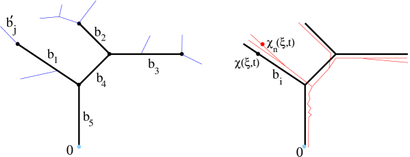
Figure 2: Left: Two finite trees, showing three maximal $\varepsilon$-good paths (thick lines) and 8 maximal $\varepsilon^{\prime}$-good paths (thin lines), for $0<\varepsilon^{\prime}<\varepsilon$. Right: proving the lower semicontinuity of the weighted irrigation cost. Given a sequence of irrigation plans $\chi_{n}\to\chi$, one can compare the cost of $\chi$ restricted to each branch $b_{i}$ with multiplicity $m(\xi,t)\geq\varepsilon$ with the corresponding costs for the approximating irrigation plans $\chi_{n}$.

Remark 3.4

In the next section we will prove that

$$\varepsilon^{\prime}\,<\,\varepsilon\qquad\Longrightarrow\qquad W^{\varepsilon}(\xi,t)~{}\leq~{}W^{\varepsilon^{\prime}}(\xi,t).$$ (3.15)

Hence the approximations $W^{\varepsilon}$ depend monotonically on $\varepsilon$. As a consequence, we can equivalently write

$$W(\xi,t)~{}=~{}\lim_{\varepsilon\to 0+}W^{\varepsilon}(\xi,t).$$ (3.16)

One should be aware that this limit may well be $+\infty$.

Remark 3.5

The assumption (A2), introduced below (2.9), guarantees that the approximation is meaningful. To see what goes wrong when (A2) fails, consider the irrigation plan $\chi:[0,M]\times\mathbb{R}_{+}\mapsto\mathbb{R}^{2}$ defined as

$$\chi(\xi,t)~{}=~{}\left\{\begin{array}[]{rl}(t\xi,t)&\hbox{if}~{}~{}t\in[0,1],\\[8.53581pt] (\xi,1)&\hbox{if}~{}~{}t\geq 1.\end{array}\right.$$

In this case the multiplicity is $m(\xi,t)=0$ for all $\xi\in[0,M]$ and $t>0$. Hence $W^{\varepsilon}(\xi,t)\equiv 0$ for all $\varepsilon>0$.

Having constructed a family of weights $W(\xi,t)$, we can now define the corresponding irrigation cost. Instead of the function $\psi(s)=s^{\alpha}$ with $0<\alpha\leq 1$, one can here consider more general cost functions $\psi:\mathbb{R}_{+}\mapsto\mathbb{R}_{+}$, satisfying the same assumptions imposed on $f$ at (1.3). As usual, an upper dot will denote a derivative w.r.t. time.

Definition 3.6

Let $f,\psi:\mathbb{R}_{+}\mapsto\mathbb{R}_{+}$ be continuous functions, both satisfying all the assumptions in (A1). Let $\chi$ be an irrigation plan satisfying (A2) and let $W=W(\xi,t)$ be the corresponding weight function, as in (3.14). If each path is parameterized by arc-length, the weighted cost is then defined as

$${\cal E}^{W,\psi}(\chi)~{}\doteq~{}\int_{0}^{M}\int_{0}^{\tau(\xi)}{\psi(W(\xi,t))\over m(\xi,t)}\,dt\,d\xi\,.$$ (3.17)

More generally, for an arbitrary parameterization of the paths $\chi(\xi,\cdot)$, the weighted cost is

$${\cal E}^{W,\psi}(\chi)~{}\doteq~{}\int_{0}^{M}\int_{0}^{\tau(\xi)}{\psi\bigl{(}W(\xi,t)\bigr{)}\over m(\xi,t)}\,|\dot{\chi}(\xi,t)|\,dt\,d\xi\,.$$ (3.18)

Remark 3.7

In the special case where $f\equiv 0$, the weight function coincides with the multiplicity: $W(\xi,t)=m(\xi,t)$. Taking $\psi(s)=s^{\alpha}$ for some $0<\alpha\leq 1$, by (2.9), this implies ${\cal E}^{W,\psi}(\chi)\geq{\cal E}^{\alpha}(\chi)$. Equality holds whenever $\chi$ has the single path property and hence $m(\xi,t)=|\chi(\xi,t)|$.

In order to compute an approximate value of the weighted cost, fix any $\varepsilon>0$ and let $\widehat{\gamma}_{1},\ldots\widehat{\gamma}_{\nu}$ be the maximal $\varepsilon$-good paths. Consider the elementary paths $\gamma_{i}$ constructed by the path splitting algorithm (PSA) at (3.7), and let $W_{i}^{\varepsilon}:[a_{i},b_{i}]\mapsto[\varepsilon,+\infty[$ be the corresponding approximate weights constructed at (3.8)–(3.10). We claim that

$${\cal E}^{W^{\varepsilon},\psi}(\chi)~{}\doteq~{}\int_{0}^{M}\int_{0}^{\tau(\xi)}{\psi(W^{\varepsilon}(\xi,t))\over m(\xi,t)}|\dot{\chi}(\xi,t)|\,dt\,d\xi~{}=~{}\sum_{i=1}^{N}\int_{a_{i}}^{b_{i}}\psi(W^{\varepsilon}_{i}(s))\,ds.$$ (3.19)

Indeed, recalling (3.12), denote by $\Omega_{\varepsilon}\subseteq[0,M]$ the set of particles such that $\tau_{\varepsilon}(\xi)>0$. By the definition of approximate weights $W^{\varepsilon}$ at (3.13), it follows

$$\int_{0}^{M}\int_{0}^{\tau(\xi)}{\psi(W^{\varepsilon}(\xi,t))\over m(\xi,t)}|\dot{\chi}(\xi,t)|\,dt\,d\xi~{}=~{}\int_{\Omega_{\varepsilon}}\int_{0}^{\tau_{\varepsilon}(\xi)}{\psi(W^{\varepsilon}(\xi,t))\over m(\xi,t)}|\dot{\chi}(\xi,t)|\,dt\,d\xi.$$ (3.20)

For each $\xi\in\Omega_{\varepsilon}$, define

$$s_{\varepsilon}(\xi)~{}\doteq~{}\int_{0}^{\tau_{\varepsilon}(\xi)}|\dot{\chi}(\xi,t)|\,dt.$$

To fix the ideas, assume that $\chi(\xi,\cdot)\Big{|}_{[0,\tau_{\varepsilon}(\xi)]}\simeq\widehat{\gamma}_{i}\Big{|}_{[0,s_{\varepsilon}(\xi)]}$ for some maximal $\varepsilon$-good path $\widehat{\gamma}_{i}$. Recalling (3.13), by a standard change of variable formula we obtain

$$\int_{0}^{\tau_{\varepsilon}(\xi)}{\psi(W^{\varepsilon}(\xi,t))\over m(\xi,t)}|\dot{\chi}(\xi,t)|\,dt~{}=~{}\int_{0}^{s_{\varepsilon}(\xi)}{\psi(\widehat{W}_{i}(s))\over\widehat{m}_{i}(s)}\,ds.$$ (3.21)

For each $s>0$ consider the set

$$\Omega_{i,k}(s)~{}\doteq~{}\Big{\{}\xi\in[0,\,M];~{}\chi(\xi,\cdot)\Big{|}_{[0,t]}\simeq\widehat{\gamma}_{i}\Big{|}_{[0,s]}\hbox{ for some }t>0,~{}t_{i,k-1}<s\leq t_{i,k}\Big{\}}.$$ (3.22)

Splitting the integral in (3.21) over the disjoint intervals $]t_{i,k-1},t_{i,k}]$ considered at (3.5), one obtains

$$\int_{0}^{s_{\varepsilon}(\xi)}{\psi(\widehat{W}_{i}(s))\over\widehat{m}_{i}(s)}\,ds~{}=~{}\sum_{k}\int_{t_{i,k-1}}^{t_{i,k}}\Big{[}{\psi(\widehat{W}_{i}(s))\over\widehat{m}_{i}(s)}\mathbf{I}_{\Omega_{i,k}(s)}(\xi)\Big{]}\,ds,$$ (3.23)

where $\mathbf{I}_{\Omega_{i,k}(s)}(\cdot)$ is the indicator function of set $\Omega_{i,k}(s)$. Observing that

$$\int_{\Omega_{\varepsilon}}\Big{[}{\psi(\widehat{W}_{i}(s))\over\widehat{m}_{i}(s)}\mathbf{I}_{\Omega_{i,k}(s)}(\xi)\Big{]}\,d\xi~{}=~{}{\psi(\widehat{W}_{i}(s))},$$

we eventually obtain (3.19).

The next lemma shows that the family of approximating weight functions $W^{\varepsilon}$ is monotonically increasing as $\varepsilon\downarrow 0$.

Lemma 3.8

Let $\chi$ be an irrigation plan and let the approximate weights $W^{\varepsilon}$ be defined as in (3.8)-(3.10). Then for any $0<\varepsilon^{\prime}<\varepsilon$ and $0\leq s<t$ one has

$$W^{\varepsilon}(\xi,t)~{}\leq~{}W^{\varepsilon^{\prime}}(\xi,t).$$ (3.24)

Proof. To prove (3.24), let $\varepsilon^{\prime}<\varepsilon$ and let $\tau_{\varepsilon^{\prime}}(\xi)\geq\tau_{\varepsilon}(\xi)$ be the corresponding stopping times in (3.12). By construction, it trivially follows

$$W^{\varepsilon}(\xi,t)~{}=~{}W^{\varepsilon^{\prime}}(\xi,t)~{}=~{}0\qquad\hbox{for all}~{}t\geq\tau_{\varepsilon^{\prime}}(\xi),$$ (3.25)

$$W^{\varepsilon}(\xi,t)~{}=~{}0~{}\leq~{}W^{\varepsilon^{\prime}}(\xi,t)\qquad\hbox{for all}~{}t\in\,]\tau_{\varepsilon}(\xi),\,\tau_{\varepsilon^{\prime}}(\xi)].$$ (3.26)

To prove the inequality in (3.24) for $t\leq\tau_{\varepsilon}(\xi)$, let $\widehat{\gamma}_{1}^{\prime},\ldots,\widehat{\gamma}^{\prime}_{\nu^{\prime}}$ be maximal $\varepsilon^{\prime}$-good paths, and let $\gamma^{\prime}_{1},\ldots,\gamma^{\prime}_{N^{\prime}}$ be the corresponding elementary paths, generated by the algorithm (PSA). By definition, the weights $W^{\varepsilon^{\prime}}$ are obtained by induction, performing the steps (i)-(ii) at (3.8)–(3.10) for the elementary paths $\gamma_{i}^{\prime}$.

Consider the functions

$$f^{\varepsilon}_{i}(w,s)~{}=~{}\left\{\begin{array}[]{cl}f(w)&\hbox{if}\quad m_{i}(s)\geq\varepsilon,\\[8.53581pt] 0&\hbox{if}\quad m_{i}(s)<\varepsilon.\end{array}\right.$$

Performing the same inductive construction, but with $f$ replaced by $f_{i}^{\varepsilon}$ on each elementary path $\gamma_{i}^{\prime}$, $i=1,\ldots,N^{\prime}$, we now recover exactly the weights $W^{\varepsilon}$. A comparison argument now yields (3.24), for all $\xi,t$. MM     

As a consequence, we have

Corollary 3.9

Let $\chi$ be an irrigation plan which satisfies the assumption (A2). Then the weighted irrigation cost in (3.17) is computed by

$${\cal E}^{W,\psi}(\chi)~{}=~{}~{}\lim_{\varepsilon\to 0+}\,\int_{0}^{M}\int_{0}^{\tau_{\varepsilon}(\xi)}{\psi(W^{\varepsilon}(\xi,t))\over m(\xi,t)}|\dot{\chi}(\xi,t)|\,dtd\xi\,.$$ (3.27)

4 Lower semicontinuity

The goal of this section is to establish the lower semicontinuity of the weighted cost functional ${\cal E}^{W,\psi}(\chi)$ w.r.t. pointwise convergence of the irrigation plans.

More precisely, consider a sequence of irrigation plans $\chi_{n}:[0,M]\times\mathbb{R}_{+}\mapsto\mathbb{R}^{d}$. We say that $\chi_{n}\to\chi$ pointwise if, for a.e. $\xi\in[0,M]$, as $n\to\infty$ one has the convergence

$$\chi_{n}(\xi,t)~{}\to~{}\chi(\xi,t)\qquad\hbox{uniformly for $t$ in compact intervals.}$$ (4.1)

In terms of the distance (2.1), this means

$$\lim_{n\to\infty}~{}d\bigl{(}\chi_{n}(\xi,\cdot),\,\chi(\xi,\cdot)\bigr{)}~{}=~{}0\qquad\hbox{for a.e. }~{}~{}\xi\in[0,M].$$

Theorem 4.1

Consider a sequence $(\chi_{n})_{n\geq 1}$ of irrigation plans, all satisfying the assumption (A2), pointwise converging to an irrigation plan $\chi$. Assume that the functions $f,\psi$ both satisfy the conditions in (A1). Then the corresponding weighted costs satisfy

$${\cal E}^{W,\psi}(\chi)~{}\leq~{}\liminf_{n\to\infty}{\cal E}^{W,\psi}(\chi_{n}).$$ (4.2)

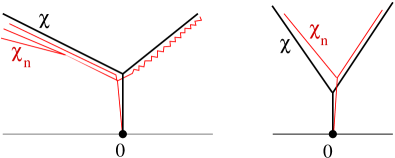
Figure 3: Left: two cases where the inequality (4.2) can be strict. (i) Paths in $\chi_{n}$ may remain separate, while in $\chi$ they all join together. (ii) Paths in $\chi_{n}$ may converge to a path in $\chi$ with strictly smaller length. Right: two cases where the weighted irrigation costs satisfy ${\cal E}^{W,\psi}(\chi_{n})<{\cal E}^{W,\psi}(\chi)$. (i) The paths in $\chi_{n}$ can be slightly shorter than those in $\chi$. (ii) Paths in $\chi_{n}$ may remain joined together for a slightly longer time than those in $\chi$. However, these differences vanish asymptotically, as $n\to\infty$.

Toward a proof, some preliminary results will be needed.

Lemma 4.2

Let $\gamma:[a,b]\mapsto\mathbb{R}^{d}$ be a Lipschitz path, and let $\varepsilon>0$. Then there exists $\delta>0$ such that, for any Lipschitz path $\gamma^{\dagger}:[a,b]\mapsto\mathbb{R}^{d}$ which satisfies

$$|\gamma^{\dagger}(s)-\gamma(s)|~{}\leq~{}\delta\qquad\qquad\hbox{for all}~{}s\in[a+\delta,\,b-\delta],$$

the length of $\gamma^{\dagger}$ is bounded below by

$$\int_{a+\delta}^{b-\delta}|\dot{\gamma}^{\dagger}(s)|\,ds~{}\geq~{}(1-\varepsilon)\int_{a}^{b}|\dot{\gamma}(s)|\,ds.$$ (4.3)

Proof. This is an immediate consequence of the lower semicontinuity of the path length.MM     

In the forthcoming analysis, it will be convenient to use a distance between two paths which is independent of their parameterization. For this purpose, following [6] we introduce

Definition 4.3

(Parameterization-free distance among paths). Given two continuous paths $\varphi_{i}:[0,\,S_{i}]\mapsto\mathbb{R}^{d}$, $i=1,2$, the distance $\delta(\varphi_{1},\varphi_{2})$ is defined as

$$\delta(\varphi_{1},\varphi_{2})~{}\doteq~{}\inf_{\eta_{1},\eta_{2}}\max_{t\in[0,1]}\Big{|}\varphi_{1}(\eta_{1}(t)-\varphi_{2}(\eta_{2}(t))\Big{|}\,,$$ (4.4)

where the infimum is taken over all couples of continuous, nondecreasing, surjective maps $\eta_{i}:[0,1]\mapsto[0,\,S_{i}].$

As shown in [6], one has

• $\delta(\varphi_{1},\varphi_{2})~{}=~{}\delta(\varphi_{2},\varphi_{1})~{}\geq~{}0\,,$

• $\delta(\varphi_{1},\varphi_{2})~{}=~{}0\hbox{ if and only if }\varphi_{1}~{}\simeq~{}\varphi_{2},$ in the sense of Definition 2.5  ,

• $\delta(\varphi_{1},\varphi_{3})~{}\leq~{}\delta(\varphi_{1},\varphi_{2})+\delta(\varphi_{2},\varphi_{3})\,.$

The proof of the following lemma is elementary, but the conclusion turns out to be crucial in the proof of lower semicontinuity of the irrigation cost.

Lemma 4.4

Let $\gamma_{i}:[0,\,\ell_{i}]\mapsto\mathbb{R}^{d}$, $i=1,2$, be two paths parametrized by arc-length. Assume that they bifurcate at some time $0\leq\tau<\min\,\{\ell_{1},\ell_{2}\}$, i.e.

$$\tau~{}=~{}\sup\Big{\{}t\geq 0\,;~{}~{}\gamma_{1}(s)=\gamma_{2}(s)\quad\hbox{for all}~{}s\in[0,t]\Big{\}}.$$

Then for any $h>0$, there exists $\sigma>0$ such that

$$\delta\Big{(}\gamma_{1}\Big{|}_{[0,s]},\gamma_{2}\Big{|}_{[0,t]}\Big{)}~{}\geq~{}\sigma,\qquad\hbox{for all}~{}s\in[\tau+h,\,\ell_{1}],\,t\in[0,\,\ell_{2}]\,.$$ (4.5)

Proof. The map $(s,t)\mapsto\delta\bigl{(}\gamma_{1}|_{[0,s]},\,\gamma_{2}|_{[0,t]}\bigr{)}$ is continuous and strictly positive on the compact domain $[\tau+h,\,\ell_{1}]\times[0,\,\ell_{2}]$. Hence it has a strictly positive minimum. MM     

In Lemma 2.13 we compared the weight $w(s)$ along a single path $\gamma$ with a sum of weights $\sum_{i}w_{i}(s)$ along a family of distinct paths $\gamma_{i}$. The next lemma extends this result to a more general configuration where the paths $\gamma_{i}$ are not necessarily disjoint, as shown in Fig. 4.

More precisely, consider an irrigation plan $\chi$ containing finitely many maximal paths $\widehat{\gamma}_{j}:[0,T]\mapsto\mathbb{R}^{d}$, $j=1,\ldots,\nu$, all parameterized by arc-length and all with the same length $T$. Let $\widehat{m}_{j}:[0,T]\mapsto\mathbb{R}^{d}$ be the (non-increasing) multiplicity function along $\widehat{\gamma}_{j}$, defined as in (3.3), and consider weights

$$\widehat{W}_{j}(T)~{}\geq~{}\widehat{m}_{j}(T)~{}>~{}0,$$ (4.6)

arbitrarily assigned at the terminal point of each maximal path. In turn, these data determine the weight functions along all paths. Namely, let $\gamma_{i}:[a_{i},b_{i}]\mapsto\mathbb{R}^{d},1\leq i\leq N$ be the corresponding elementary paths, constructed by the Path Splitting Algorithm (PSA). By backward induction we can now construct the weights $W_{i}$ along each elementary path, in a similar way as in (3.8)–(3.10).

• For every index $i$ such that $b_{i}=T$, the weight $W_{i}:[a_{i},b_{i}]\mapsto\mathbb{R}_{+}$ along the elementary path $\gamma_{i}$ is computed by solving

  $$w(t)~{}=~{}\int_{t}^{b_{i}}f(w(s))\,ds+m_{i}(t)+\bigl{[}\widehat{W}_{j(i)}(T)-m_{i}(T)\bigr{]}\,,\qquad\qquad t\in\,]a_{i},T].$$ (4.7)

  Here $\widehat{\gamma}_{j(i)}$ is the unique maximal path that contains $\gamma_{i}$ as its restriction to $[a_{i},b_{i}]=[a_{i},T]$.

• If $b_{i}<T$, the weight $W_{i}:[a_{i},b_{i}]\mapsto\mathbb{R}_{+}$ along the elementary path $\gamma_{i}$ is then defined to be the solution of

  $$w(t)~{}=~{}\int_{t}^{b_{i}}f(w(s))\,ds+m_{i}(t)+\left[\sum_{k\in{\cal O}(i)}W_{k}(a_{k}+)-\sum_{k\in{\cal O}(i)}m_{k}(a_{k}+)\right],\qquad t\in\,]a_{i},b_{i}].$$ (4.8)

  As in (3.10), here the summations range over all elementary paths $\gamma_{k}$ that originate from the tip of $\gamma_{i}$.

Figure 4: The two configurations compared in Lemma 4.5. For every $t\in[0,T]$, the sum of the weight functions $W_{i}(t)$ along a family of maximal paths $\widehat{\gamma}_{i}$ is compared with a single weight $W(t)$, satisfying the ODE (4.10).

Lemma 4.5

Let the weights $W_{i}:[a_{i},b_{i}]\mapsto\mathbb{R}_{+}$ be constructed as above. Given any constant $\widehat{W}$ such that

$$0~{}<~{}\widehat{W}~{}\leq~{}\sum_{j=1}^{\nu}\widehat{W}_{j}(T)\,,$$ (4.9)

let $W:[0,T]\mapsto\mathbb{R}$ be the solution to the backward Cauchy problem

$$\dot{W}(t)~{}=~{}-f(W(t)),\qquad\qquad W(T)\,=\,\widehat{W}.$$ (4.10)

Then for all $t\in\,]0,T]$ one has

$$W(t)~{}\leq~{}\sum_{i\in I(t)}W_{i}(t)\,,$$ (4.11)

where $I(t)$ denotes the set of indices $i\in\{1,\ldots,N\}$ such that $a_{i}<t\leq b_{i}$. As a consequence,

$$\int_{0}^{T}\psi(W(t))\,dt~{}\leq~{}\sum_{i=1}^{N}\int_{a_{i}}^{b_{i}}\psi(W_{i}(t))\,dt\,.$$ (4.12)

Proof. Let $0<t_{1}<\cdots<t_{q}=T$ be the times where two or more maximal paths bifurcate. The proof will achieved by backward induction on $p=1,2,\ldots,q$. 1. For $t\in]t_{q-1},t_{q}]=\,]t_{q-1},T]$, the above definition implies $I(t)=I(T)$. By (4.9) it follows

$$\sum_{i\in I(T)}W_{i}(T)~{}\geq~{}\widehat{W}\,.$$ (4.13)

For each $i\in I(T)$, $t\in\,]t_{q-1},T]$, by (4.7) it follows

$$W_{i}(t)~{}=~{}\int_{t}^{t_{q}}f(W_{i}(s))\,ds+W_{i}(T)+\left[m_{i}(t)-m_{i}(T)\right]$$ (4.14)

On the other hand,

$$W(t)~{}=~{}\int_{t}^{t_{q}}f(W(s))\,ds+\widehat{W}\,.$$ (4.15)

Because of (4.13) we can apply Lemma 2.13 and conclude that

$$\sum_{i\in{\cal I}(T)}W_{i}(t)~{}\geq~{}W(t),\qquad\hbox{for all}~{}t\in\,]t_{q-1},T].$$ (4.16)

2. Next, assume that that the inequality (4.11) has been proved for all $t\in\,]t_{p},T]$, for some $1\leq p<q$. We claim that it also holds for $t\in\,]t_{p-1},t_{p}]$.

Indeed, since the solution $W$ of (4.10) is continuous while all weights $W_{i}$ are non-increasing, the inductive assumption yields

$$\sum_{i\in{\cal I}(t_{p})}W_{i}(t_{p})~{}\geq~{}W(t_{p})\,.$$ (4.17)

For each $i\in I(t_{p})$, $t\in\,]t_{p-1},t_{p}]$, we then have

$$\begin{array}[]{c}\displaystyle W_{i}(t)~{}=~{}\int^{t_{p}}_{t}f(W_{i}(s))\,ds+W_{i}(t_{p})+\left[m_{i}(t)-m_{i}(t_{p})\right]\,,\\[8.53581pt] \displaystyle W(t)~{}=~{}\int_{t}^{t_{p}}f(W(s))\,ds+W(t_{p})\end{array}$$ (4.18)

Because of (4.17) we can again apply Lemma 2.13 and conclude

$$\sum_{i\in{\cal I}(t_{p})}W_{i}(t)~{}\geq~{}W(t),\qquad\hbox{for all}~{}t\in(t_{p-1},\,t_{p}].$$ (4.19)

By induction on $p$, this yields a proof of (4.11). 3. Since $\psi$ satisfies the assumption (A2), from (4.11) it follows

$$\begin{array}[]{l}\displaystyle\sum_{i=1}^{N}\int_{a_{i}}^{b_{i}}\psi(W_{i}(t))\,dt~{}=~{}\sum_{p=1}^{q}\sum_{i\in I(t_{p})}\int_{t_{p-1}}^{t_{p}}\psi(W_{i}(t))\,dt\\[8.53581pt] \displaystyle\quad\geq~{}\sum_{p=1}^{q}\int_{t_{p-1}}^{t_{p}}\psi(W(t))\,dt~{}=~{}\int_{0}^{T}\psi(W(t))\,dt\end{array}$$ (4.20)

Hence (4.12) holds. MM     

Remark 4.6

In Lemma 4.5 we assumed that all maximal paths $\widehat{\gamma}_{j}$ had the same length $T$. The same conclusions (4.11)-(4.12) remain valid if each maximal path $\widehat{\gamma}_{j}:[0,T_{j}]\mapsto\mathbb{R}^{d}$ is defined on an interval of length $T_{j}\geq T$, replacing (4.9) with

$$\widehat{W}~{}\leq~{}\sum_{j=1}^{\nu}\widehat{W}_{j}(T_{j}).$$ (4.21)

To prove this, it suffices to consider the restriction of each $\widehat{\gamma}_{j}$ to the sub-interval $[0,T]$, and observe that (4.21) implies (4.9), because the weight functions are non-increasing,

After these preliminaries, we are now ready to give a proof of the main result of this section, in several steps.

Proof of Theorem 4.1.

1. Without loss of generality, we can assume that all paths $\chi_{n}(\xi,\cdot)$ are parameterized by arc-length. As a consequence, for each $\xi\in[0,\,M]$, the limit paths $\chi(\xi,\cdot)$ will be 1-Lipschitz, but not necessarily parameterized by arc-length.

Fix any $\varepsilon_{0}>0$. Let $\tau_{\varepsilon_{0}}$ be the corresponding stopping time as in (3.12), and define the truncated irrigation plan

$$\chi^{\varepsilon_{0}}(\xi,t)~{}\doteq~{}\left\{\begin{array}[]{cl}\chi(\xi,t)&\hbox{if}\qquad t\leq\tau_{\varepsilon_{0}}(\xi),\\[11.38109pt] \chi(\xi,\tau_{\varepsilon_{0}}(\xi))&\hbox{if}\qquad t>\tau_{\varepsilon_{0}}(\xi).\end{array}\right.$$ (4.22)

Using Corollary 3.9, the theorem will be proved by showing that

$${\cal E}^{W,\psi}(\chi^{\varepsilon_{0}})~{}\leq~{}\liminf_{n\to\infty}{\cal E}^{W,\psi}(\chi_{n}).$$ (4.23)

2. For each $\xi\in[0,\,M]$, in order to re-parameterize the limit path $\chi(\xi,\cdot)$ in terms of arc-length, let

$$s(\xi,t)~{}\doteq~{}\int_{0}^{t}|\dot{\chi}(\xi,r)|\,dr.$$ (4.24)

A left-continuous inverse of $s(\xi,\cdot)$, taking values in $\mathbb{R}_{+}\cup\{+\infty\}$, can be defined as

$$\eta(\xi,s)~{}\doteq~{}\inf\Big{\{}t~{}\geq~{}0;~{}s(\xi,t)~{}=~{}s\Big{\}}\,.$$ (4.25)

The map

$$s~{}\mapsto~{}\chi(\xi,\eta(\xi,s))$$ (4.26)

now provides the arc-length parameterization of $\chi(\xi,\cdot)$. We observe that, for each $s$, the map $\xi\mapsto\eta(\xi,s)$ is measurable. Moreover, since $|\dot{\chi}(\xi,t)|\leq 1$, one has

$$\eta(\xi,s_{2})-\eta(\xi,s_{1})~{}\geq~{}s_{2}-s_{1}\qquad\hbox{for all}~{}0\leq s_{1}<s_{2}\,.$$ (4.27)

3. Next, let $\widehat{\gamma}_{1},\ldots,\widehat{\gamma}_{\nu}$ be the maximal $\varepsilon_{0}$-good paths for the irrigation plan $\chi$. As before, we assume that each $\widehat{\gamma}_{j}:[0,\widehat{\ell}_{j}]\mapsto\mathbb{R}^{d}$ is parameterized by arc-length. For $s\in\,]0,\widehat{\ell}_{j}]$, let

$$\widehat{\Omega}_{j}(s)~{}\doteq~{}\left\{\xi\in[0,M];\quad\chi(\xi,\cdot)\Big{|}_{[0,t]}\simeq\widehat{\gamma}_{j}\Big{|}_{[0,s]}~{}\hbox{ for some }t>0\right\}$$

be the set of particles whose trajectory follows the path $\widehat{\gamma}_{j}$, at least up to the point $\widehat{\gamma}_{j}(s)$.

Implementing the algorithm (PSA) described at (3.5)–(3.7), these maximal paths can be split into finitely many elementary paths $\gamma_{1},\ldots,\gamma_{N}$. By construction, each $\gamma_{i}:[a_{i},b_{i}]\mapsto\mathbb{R}^{d}$, $1\leq i\leq N$ is the restriction of some $\widehat{\gamma}_{j}$ to a subinterval $[a_{i},b_{i}]$. We then define

$$\Omega_{i}(s)~{}\doteq~{}\widehat{\Omega}_{j}(s)\qquad\hbox{for all}~{}s\in\,[a_{i},b_{i}].$$ (4.28)

The multiplicity function $m_{i}:[a_{i},b_{i}]\mapsto\mathbb{R}_{+}$ along the elementary path $\gamma_{i}$ is then computed by

$$m_{i}(s)~{}=~{}\hbox{meas}(\Omega_{i}(s))\,,\qquad s\in\,[a_{i},b_{i}]\,.$$ (4.29)

According to (3.19), the approximate weighted irrigation cost is computed by a sum over all elementary paths:

$$E^{W,\psi}(\chi^{\varepsilon_{0}})~{}=~{}\sum_{i=1}^{N}\int_{a_{i}}^{b_{i}}\psi(W_{i}^{\varepsilon_{0}}(s))\,ds,$$ (4.30)

where the weights $W^{\varepsilon_{0}}_{i}$ are determined as in (3.8)–(3.10).

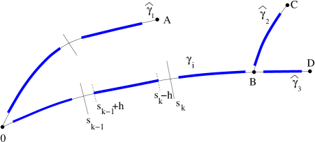
Figure 5: Proving the lower semicontinuity of the weighted irrigation cost, steps 3-4. Here $\widehat{\gamma}_{1},\widehat{\gamma}_{2},\widehat{\gamma}_{3}$ are maximal $\varepsilon_{0}$-good paths of $\chi$, while $\gamma_{i}:[a_{i},b_{i}]\mapsto\mathbb{R}^{d}$, with endpoints $0,B$, is an elementary path produced by the algorithm (PSA). The path $\gamma_{i}$ is further partitioned, taking subintervals $[s_{k-1},s_{k}]$ of length $\leq\delta$. We then approximate the multiplicity $m_{i}(s)$ with a piecewise constant function $\widetilde{m}_{i}$, as in (4.32) and replace $f$ with $f^{h}$ as in (4.33). By choosing the constants $\delta,\delta_{0},h>0$ sufficiently small, the new weight $\widetilde{W}_{i}$ determined by (4.35) can be kept arbitrarily close to the original weight $W_{i}^{\varepsilon_{0}}$.

4. We claim that it is possible to replace the multiplicity functions $m_{i}$ by strictly smaller piecewise constant functions $\widetilde{m}_{i}$, producing a very small change in the weights $W^{\varepsilon_{0}}_{i}$. More precisely, for each $i\in\{1,\ldots,N\}$, choose $\delta>0$ and insert the times (see Fig. 5)

$$a_{i}\,=\,s_{0}\,<\,s_{1}\,<\,\cdots\,<\,s_{n(i)}\,=\,b_{i}\,,$$ (4.31)

so that $s_{k}-s_{k-1}\leq\delta$ for every $k=1,\ldots,n(i)$. For a given $\delta_{0}>0$, with $\delta_{0}<\varepsilon_{0}$, we then define the piecewise constant function

$$\widetilde{m}_{i}(t)~{}=~{}m_{i}(s_{k})-\delta_{0}\qquad\hbox{for all}~{}t\in\,]s_{k-1},s_{k}].$$ (4.32)

Since $s\mapsto m_{i}(s)\in[\varepsilon_{0},+\infty[\,$ is non-increasing, we clearly have $0<\widetilde{m}_{i}(t)<m(t)$ for all $t\in\,]a_{i},b_{i}]$. Next, given another constant $h>0$, with $h<\!<\delta$, we define

$$f^{h}(t,\omega)~{}\doteq~{}\left\{\begin{array}[]{cl}f(\omega)&\qquad\hbox{if}~{}~{}~{}t\in[s_{k-1}+h,~{}s_{k}-h],\quad 1\leq k\leq n(i),\\[8.53581pt] 0&\qquad\hbox{otherwise.}\end{array}\right.$$ (4.33)

We claim that, for any $\varepsilon>0$, one can choose the above constants $\delta,\delta_{0},h>0$ small enough so that, replacing the multiplicities $m_{i}$ with $\widetilde{m}_{i}$, and replacing $f$ with $f^{h}$, the corresponding weights $\widetilde{W}_{i}$ satisfy

$$\|W_{i}^{\varepsilon_{0}}-\widetilde{W}_{i}\|_{{\bf L}^{1}([a_{i},b_{i}])}~{}<~{}\varepsilon,\qquad\qquad|W_{i}^{\varepsilon_{0}}(a_{i}+)-\widetilde{W}_{i}(a_{i}+)|\,<\,\varepsilon\,.$$ (4.34)

Indeed, recalling (1.5) consider first the case $i\in{\cal I}_{1}$, so that $\gamma_{i}$ is one of the outer-most branches. Then the weight $W_{i}^{\varepsilon_{0}}$ is obtained by solving (3.8), while $\widetilde{W}_{i}$ provides a solution to

$$w(t)~{}=~{}\int_{t}^{b_{i}}f^{h}(s,w(s))\,ds+\widetilde{m}_{i}(t),\qquad\qquad t\in\,]a_{i},b_{i}].$$ (4.35)

By choosing $\delta,\delta_{0},h>0$ sufficiently small, we can make the differences

$$\|m_{i}-\widetilde{m}_{i}\|_{{\bf L}^{1}([a_{i},b_{i}])}\,,\qquad|m_{i}(a_{i}+)-\widetilde{m}_{i}(a_{i}+)|\,,\qquad\hbox{meas}\left([a_{i},\,b_{i}]\setminus\bigcup_{k=1}^{n(i)}[s_{k-1}+h,\,s_{k}-h]\right)$$

as small as we like. The estimate (4.34) thus follows from part (iii) of Lemma 2.12.

The case $i\in{\cal I}_{p}$ for $p>1$ is proved in the same way, by induction on $p$. In view of (4.23) and (4.30), to prove the theorem it thus suffices to show that, for any given $\delta,\delta_{0},h>0$, the corresponding weights $\widetilde{W}_{i}$ satisfy

$$\sum_{i=1}^{N}\int_{a_{i}}^{b_{i}}\psi(\widetilde{W}_{i}(s))\,ds~{}\leq~{}\liminf_{n\to\infty}{\cal E}^{W,\psi}(\chi_{n}).$$ (4.36)

5. Consider again the arrival time $\xi\mapsto\tau(\xi)$ introduced in Definition 2.1. For any $\varepsilon>0$, by Corollary 2.4 there is a compact set $\Omega_{\varepsilon}\subseteq[0,M]$, with

$$\hbox{meas}\,\bigl{(}[0,M]\setminus\Omega_{\varepsilon}\bigr{)}~{}<~{}\varepsilon\,,$$ (4.37)

on which that map $\tau(\cdot)$ is continuous. Hence

$$\max_{\xi\in\Omega_{\varepsilon}}~{}\tau(\xi)~{}\leq~{}\kappa$$ (4.38)

for some constant $\kappa$. By (4.1) and Egoroff’s theorem, by slightly shrinking the compact set $\Omega_{\varepsilon}$, we can assume that (4.37) still holds, together with

$$\lim_{n\to\infty}\sup_{\xi\in\Omega_{\varepsilon}}\|\chi(\xi,\cdot)-\chi_{n}(\xi,\cdot)\|_{\mathbf{L}^{\infty}([0,\kappa])}~{}=~{}0\,.$$ (4.39)

In addition, calling $\tau^{n}(\xi)$ the smallest time $\tau$ such that $\chi_{n}(\xi,\cdot)$ is constant for $t\geq\tau$, by further shrinking $\Omega_{\varepsilon}$ we can also assume

$$\liminf_{n\to\infty}\inf_{\xi\in\Omega_{\varepsilon}}\left[\tau^{n}(\xi)-\tau(\xi)\right]~{}\geq~{}0.$$ (4.40)

Indeed, since

$$\liminf_{n\to\infty}\tau^{n}(\xi)~{}\geq~{}\tau(\xi),$$ (4.41)

it follows that the non-decreasing sequence

$$\widehat{\tau}^{n}(\xi)~{}\doteq~{}\inf_{k\geq n}\tau^{k}(\xi)$$

converges to a limit

$$\lim_{n\to\infty}\widehat{\tau}^{n}(\xi)~{}=~{}\tau^{\infty}(\xi)~{}\geq~{}\tau(\xi)$$

for a.e. $\xi\in[0,M]$. Again by Egoroff’s theorem we can choose a large subset $\Omega_{\varepsilon}\subset[0,M]$ where the pointwise convergence is uniform. This yields (4.40).

Furthermore, since each $\chi_{n}$ satisfies the assumption (A2), we can choose $\varepsilon_{n}>0$ small enough so that the following holds. Defining the stopping time

$$\tau^{n}_{\varepsilon_{n}}(\xi)~{}\doteq~{}\sup\,\bigl{\{}t\geq 0\,;~{}~{}m_{n}(\xi,t)\geq\varepsilon_{n}\bigr{\}},$$ (4.42)

by possibly further shrinking the set $\Omega_{\varepsilon}$ in (4.37) one has

$$\tau^{n}_{\varepsilon_{n}}(\xi)~{}\geq~{}\tau^{n}(\xi)-{h\over 2}\qquad\hbox{for all}~{}\xi\in\Omega_{\varepsilon},~{}~{}n\geq 1\,.$$ (4.43)

6. Let $\widehat{\gamma}^{\prime}_{1},\ldots,\widehat{\gamma}^{\prime}_{\nu^{\prime}}$ be the maximal $\varepsilon_{n}$-good paths in $\chi_{n}$, and let $\gamma^{\prime}_{1},\ldots,\gamma_{N^{\prime}}^{\prime}$ be the elementary paths constructed by the algorithm (PSA). As in step 3, for each $\widehat{\gamma}_{j}^{\prime}:[0,\hat{\ell}_{j}^{\prime}]\mapsto\mathbb{R}^{d}$ we define

$$\begin{array}[]{rl}\widehat{\Omega}_{j}^{\prime}(s)&\displaystyle\doteq~{}\left\{\xi\in[0,M];~{}\chi_{n}(\xi,\cdot)\Big{|}_{[0,t]}\simeq\widehat{\gamma}_{j}^{\prime}\Big{|}_{[0,s]}\hbox{ for some }t>0\right\}\\[11.38109pt] &=~{}\displaystyle\Big{\{}\xi\in[0,M];~{}\chi_{n}(\xi,t)=\widehat{\gamma}_{j}^{\prime}(t),~{}\hbox{for all}~{}t\in[0,s]\Big{\}}.\end{array}$$ (4.44)

This is the set of particles whose trajectory follows the maximal path $\widehat{\gamma}_{j}^{\prime}$, at least up to time $s$. Notice that the last identity holds because $\widehat{\gamma}_{j}^{\prime}$ and $\chi_{n}(\xi,\cdot)$ are both parameterized by arc-length. By construction, each elementary path $\gamma_{i}^{\prime}:[a_{i}^{\prime},b^{\prime}_{i}]\mapsto\mathbb{R}^{d}$, $1\leq i\leq N^{\prime}$ is the restriction of some $\widehat{\gamma}_{j}^{\prime}$ to a subinterval $[a^{\prime}_{i},b^{\prime}_{i}]$. We then define

$$\Omega^{\prime}_{i}(s)~{}\doteq~{}\widehat{\Omega}_{j}^{\prime}(s)\qquad\hbox{for all}~{}s\in\,[a^{\prime}_{i},b^{\prime}_{i}].$$ (4.45)

7. Now consider a particle $\xi\in\Omega_{i}(s_{k})\cap\Omega_{\varepsilon}$, so that the path $t\mapsto\chi(\xi,t)$ reaches the point $\gamma_{i}(s_{k})$ at some time $t=\eta(\xi,s_{k})$. This implies $\tau(\xi)\geq\eta(\xi,s_{k})$. Hence by (4.40) we have

$$\tau^{n}(\xi)~{}>~{}\eta(\xi,s_{k})-{h\over 2}$$

for all $n$ large enough. In turn, choosing $\varepsilon_{n}>0$ sufficiently small, by (4.43) it follows

$$\tau^{n}_{\varepsilon_{n}}(\xi)~{}\geq~{}\tau^{n}(\xi)-{h\over 2}~{}>~{}\eta(\xi,s_{k})-h~{}\geq~{}\eta(\xi,s_{k}-h).$$

Otherwise stated, by further slightly shrinking the compact set $\Omega_{\varepsilon}$ in (4.37), for any $h>0$ we can thus achieve the implication

$$\xi~{}\in~{}\Omega_{i}(s_{k})\cap\Omega_{\varepsilon}\qquad\Longrightarrow\qquad\eta(\xi,s_{k}-h)~{}<~{}\tau^{n}_{\varepsilon_{n}}(\xi),$$ (4.46)

for all $n$ sufficiently large. 8. We observe that two particles $\xi,\widetilde{\xi}$, which have the same trajectory in the irrigation plan $\chi$, may be sent along different paths by the irrigation plan $\chi_{n}$. To account for this fact, recalling (4.28) and (4.45), for a fixed $n\geq 1$ we define

$$A_{i}^{j}(s_{k})~{}\doteq~{}\left\{\xi\in\Omega_{\varepsilon}\cap\Omega_{i}(s_{k});~{}\chi_{n}(\xi,t)~{}=~{}\widehat{\gamma}_{j}^{\prime}(t),~{}\hbox{for all}~{}0\leq t\leq\eta(\xi,s_{k}-h)\right\}.$$ (4.47)

In other words, $A_{i}^{j}(s_{k})$ is the set of particles $\xi\in\Omega_{\varepsilon}$ such that:

• By the irrigation plan $\chi$ they are moved along the $\varepsilon_{0}$-good elementary path $\gamma_{i}$, at least up to the point $\gamma_{i}(s_{k})$.

• By the irrigation plan $\chi_{n}$ they are moved along the $\varepsilon_{n}$-good maximal path $\widehat{\gamma}_{j}^{\prime}$, at least up to point $\widehat{\gamma}_{j}^{\prime}\bigl{(}\eta(\xi,s_{k}-h)\bigr{)}$.

Using Lusin’s theorem and by possibly shrinking the compact domain $\Omega_{\varepsilon}\subseteq[0,M]$, in addition to (4.37) we can assume that, restricted to each $A_{i}^{j}(s_{k})$, the two maps

$$\eta(\cdot,s_{k}-h):A_{i}^{j}(s_{k})\mapsto\mathbb{R}_{+},\qquad\qquad\eta(\cdot,s_{k-1}+h):A_{i}^{j}(s_{k})\mapsto\mathbb{R}_{+}$$

are continuous. 9. The set of paths

$$\gamma_{i,k}~{}\doteq~{}\gamma_{i}\Big{|}_{[s_{k-1},\,s_{k}]}$$ (4.48)

comes with an obvious partial ordering. Namely, we define

$$(i,k)~{}\preceq~{}(i^{\dagger},k^{\dagger})$$ (4.49)

if the two elementary paths $\gamma_{i},\gamma_{i^{\dagger}}$ for the irrigation plan $\chi$ are both contained in some $\varepsilon_{0}$-good maximal path $\widehat{\gamma}_{j}$, and moreover $s_{k}\leq s_{k^{\dagger}}$.

As shown in Fig. 6, to each portion $\gamma_{i,k}$ of the elementary path $\gamma_{i}$ in the irrigation plan $\chi$ we shall associate a family $\{\gamma^{\sharp}_{l}\}$ of paths in the irrigation plan $\chi_{n}$, and compare the corresponding costs. For this purpose, assuming $A_{i}^{j}(s_{k})\not=\emptyset$, we define

$$s_{k+}^{i,j}~{}\doteq~{}\inf_{\xi\in A_{i}^{j}(s_{k})}\eta(\xi,s_{k}-h),\qquad\qquad s_{k-}^{i,j}~{}\doteq~{}\inf_{\xi\in A_{i}^{j}(s_{k})}\eta(\xi,s_{k-1}+h).$$ (4.50)

Notice that, by (4.27), one has

$$s_{k+}^{i,j}-s_{k-}^{i,j}~{}\geq~{}s_{k}-s_{k-1}-2h.$$ (4.51)

For each $i,j,k$ such that $A_{i}^{j}(s_{k})$ is non-empty, we now consider all the paths $\gamma^{\sharp}_{l}:[a^{\sharp}_{l},\,b^{\sharp}_{l}]\mapsto\mathbb{R}^{d}$, obtained as follows. Consider all the $\varepsilon_{n}$-good elementary paths $\gamma_{p}^{\prime}:[a^{\prime}_{p},b^{\prime}_{p}]\mapsto\mathbb{R}^{d}$ of $\chi_{n}$. which are contained in the maximal path $\widehat{\gamma}_{j}^{\prime}$. We then take $\gamma_{l}^{\sharp}$ to be the restriction of $\gamma_{p}^{\prime}$ to the subinterval

$$[a^{\sharp}_{l},\,b^{\sharp}_{l}]~{}\doteq~{}[a^{\prime}_{p},b^{\prime}_{p}]\,\cap\,[s_{k-}^{i,j}\,,s_{k+}^{i,j}].$$ (4.52)

Call $\Gamma_{i,k}$ the collection of all such paths $\gamma^{\sharp}_{l}$, as $j$ varies among all the maximal $\varepsilon_{n}$-good paths of $\chi_{n}$, with $A_{i}^{j}(s_{k})\not=\emptyset$.

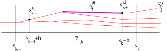
Figure 6: To compare the cost of the irrigation plans $\chi$ and $\chi_{n}$, to the portion of the $\varepsilon_{0}$-good elementary path $\gamma_{i}:[s_{k-1}+h,s_{k}-h]\mapsto\mathbb{R}^{d}$ we associate a family of $\varepsilon_{n}$-good paths $\gamma^{\sharp}_{l}$ in $\chi_{n}$.

10. Let $m^{\sharp}_{l}:[a^{\sharp}_{l},b^{\sharp}_{l}]\mapsto\mathbb{R}_{+}$ be the multiplicity of the path $\gamma^{\sharp}_{l}$ in the irrigation plan $\chi_{n}$. We claim that, choosing $\delta_{0}=\varepsilon$ in (4.32), for all $n$ large enough the piecewise constant multiplicity $\widetilde{m}_{i}$ defined at (4.32) satisfies

$$\widetilde{m}_{i}(t)~{}=~{}\widetilde{m}_{i}(s_{k}-h)~{}\doteq~{}m_{i}(s_{k})-\varepsilon~{}<~{}\sum_{\gamma_{l}^{\sharp}\in\Gamma_{i,k},~{}b^{\sharp}_{l}=s_{k+}^{i,j}}m^{\sharp}_{l}(b_{l}^{\sharp})$$ (4.53)

for all $t\in\,]s_{k-1},s_{k}]$. Indeed, in view of (4.46)-(4.47), for each $\xi\in\Omega_{i}(s_{k})\cap\Omega_{\varepsilon}$, there is some maximal path $\widehat{\gamma}_{j}^{\prime}$ such that

$$\chi_{n}(\xi,t)~{}=~{}\widehat{\gamma}_{j}^{\prime}(t),\qquad\hbox{for all}~{}t\in[0,\,\eta(\xi,s_{k}-h)].$$ (4.54)

By (4.50) we know that $\eta(\xi,s_{k}-h)\geq s_{k+}^{i,j}$. Hence (4.54) implies $\xi\in\widehat{\Omega}^{\prime}_{j}(s_{k+}^{i,j})$. Therefore

$$\widetilde{m}_{i}(s_{k}-h)~{}=~{}\hbox{meas}(\Omega_{i}(s_{k}))-\varepsilon~{}<~{}\hbox{meas}\Big{(}\Omega_{i}(s_{k})\cap\Omega_{\varepsilon}\Big{)}~{}<~{}\sum_{\gamma_{l}^{\sharp}\in\Gamma_{i,k},~{}b^{\sharp}_{l}=s_{k+}^{i,j}}m^{\sharp}_{l}(b_{l}^{\sharp}).$$ (4.55)

11. Toward a proof of (4.36), a key observation is the following. If two particles $\xi,\widetilde{\xi}$ are sent by $\chi$ along two maximal paths $\widehat{\gamma}_{i},\widehat{\gamma}_{j}$ which bifurcate at a some time $\tau_{ij}$, then, for all $n$ large enough, the irrigation plan $\chi_{n}$ must send these two particles along distinct paths as well. In this step we prove a precise estimate in this direction.

Let $\widehat{\gamma}_{1},\ldots,\widehat{\gamma}_{\nu}$ be the maximal $\varepsilon_{0}$-good paths for the irrigation plan $\chi$. For any given $h>0$, by Lemma 4.4 one can find $\sigma>0$ such that

$$\delta\left(\widehat{\gamma}_{i}\Big{|}_{[0,s]},\widehat{\gamma}_{j}\Big{|}_{[0,t]}\right)~{}\geq~{}\sigma\,,\qquad\hbox{for all}~{}i\neq j\,,~{}s\in[\tau_{ij}+h,\,\hat{\ell}_{i}],~{}t\in[0,\,\hat{\ell}_{j}]\,.$$ (4.56)

Here $\tau_{ij}$ is the time where the maximal paths $\widehat{\gamma}_{i}$ and $\widehat{\gamma}_{j}$ bifurcate, as defined at (3.4).

On the other hand, by (4.39), for all $n$ sufficiently large one has

$$\sup_{\xi\in\Omega_{\varepsilon}}\|\chi(\xi,\cdot)-\chi_{n}(\xi,\cdot)\|_{\mathbf{L}^{\infty}([0,\kappa])}~{}<~{}{\sigma\over 3}\,,$$ (4.57)

where $\sigma$ is the constant in (4.56).

Consider two particles $\xi,\widetilde{\xi}\in\Omega_{\varepsilon}$ which are sent by $\chi$ along the two distinct maximal paths $\widehat{\gamma}_{i},\widehat{\gamma}_{j}$. More precisely, recalling the definition (4.44), assume that for some $h>0$

$$\xi\,\in\,\widehat{\Omega}_{i}(\tau_{ij}+h)\cap\Omega_{\varepsilon},\qquad\qquad\widetilde{\xi}\in\widehat{\Omega}_{j}(\tau_{ij}+h)\cap\Omega_{\varepsilon}\,,$$

Without loss of generality, assume

$$T~{}\doteq~{}\eta(\xi,\tau_{ij}+h)~{}\leq~{}\eta(\widetilde{\xi},\tau_{ij}+h).$$

Recalling the notation used at (4.24), we can now find $\tau\doteq s(\widetilde{\xi},T)\leq\hat{\ell}_{j}$, such that by (4.56) and (4.57)

$$\begin{array}[]{rl}\sigma&\leq~{}\displaystyle\delta\Big{(}\widehat{\gamma}_{i}\Big{|}_{[0,\tau_{ij}+h]},\widehat{\gamma}_{j}\Big{|}_{[0,\tau]}\Big{)}~{}=~{}\delta\Big{(}\chi(\xi,\cdot)\Big{|}_{[0,T]},\chi(\widetilde{\xi},\cdot)\Big{|}_{[0,T]}\Big{)}\\[11.38109pt] &\displaystyle\leq~{}\bigl{\|}\chi(\xi,\cdot)-\chi_{n}(\xi,\cdot)\|_{{\bf L}^{\infty}([0,T])}+\delta\Big{(}\chi_{n}(\xi,\cdot)\Big{|}_{[0,T]},\chi_{n}(\widetilde{\xi},\cdot)\Big{|}_{[0,T]}\Big{)}\\[11.38109pt] &\qquad\displaystyle+\bigl{\|}\chi(\widetilde{\xi},\cdot)-\chi_{n}(\widetilde{\xi},\cdot)\|_{{\bf L}^{\infty}([0,T])}\\[8.53581pt] &\displaystyle\leq~{}\delta\Big{(}\chi_{n}(\xi,\cdot)\Big{|}_{[0,T]},\chi_{n}(\widetilde{\xi},\cdot)\Big{|}_{[0,T]}\Big{)}+{2\sigma\over 3}\,.\end{array}$$ (4.58)

This proves that the two paths $\chi_{n}(\xi,\cdot)$ and $\chi_{n}(\widetilde{\xi},\cdot)$, which are parameterized by arc-length, cannot coincide over the entire interval $[0,T]$. 12. We are finally ready to prove (4.36). Let $\varepsilon>0$ be given. Since the weights $\widetilde{W}_{i}$ are uniformly bounded, by choosing $h>0$ small enough for every $i=1,\ldots,N$ we achieve

$$\int_{a_{i}}^{b_{i}}\psi(\widetilde{W}_{i}(s))\,ds-\sum_{k=1}^{n(i)}\int_{s_{k-1}+h}^{s_{k}-h}\psi(\widetilde{W}_{i}(s))\,ds~{}<~{}{\varepsilon\over N}\,.$$ (4.59)

Since $\varepsilon>0$ is arbitrary, to prove (4.36), it is thus suffices to show that

$$\sum_{i=1}^{N}\sum_{k=1}^{n(i)}\int_{s_{k-1}+h}^{s_{k}-h}\psi(\widetilde{W}_{i}(s))\,ds~{}\leq~{}\liminf_{n\to\infty}{\cal E}^{W,\psi}(\chi_{n}).$$ (4.60)

As shown in step 9, there is a map

$$\gamma_{i,k}~{}\mapsto~{}\Gamma_{i,k}~{}\doteq~{}\bigl{\{}\gamma^{\sharp}_{l}\,;~{}l=l(i,j,k)\bigr{\}},$$ (4.61)

which associates to the portion of elementary path $\gamma_{i,k}$ of $\chi$ a corresponding family of $\varepsilon_{n}$-good paths of $\chi_{n}$, as in Fig. 6. Using the ordering (4.49), by induction on $(i,k)$ we will show that

$$\int_{s_{k-1}+h}^{s_{k}-h}\psi(\widetilde{W}_{i}(s))\,ds~{}\leq~{}\sum_{\gamma_{l}^{\sharp}\in\Gamma_{i,k}}\int_{a_{l}^{\sharp}}^{b_{l}^{\sharp}}\psi(W_{l}^{\sharp}(s))\,ds,$$ (4.62)

for every $(i,k)$. By showing that paths $\gamma^{\sharp}_{l}$ belonging to distinct families $\Gamma_{i,k}$, $\Gamma_{i^{\dagger},k^{\dagger}}$ are disjoint, we will conclude

$$\sum_{i=1}^{N}\sum_{k=1}^{n(i)}\int_{s_{k-1}+h}^{s_{k}-h}\psi(\widetilde{W}_{i}(s))\,ds~{}\leq~{}\sum_{i=1}^{N}\sum_{k=1}^{n(i)}\sum_{\gamma_{l}^{\sharp}\in\Gamma_{i,k}}\int_{a_{l}^{\sharp}}^{b_{l}^{\sharp}}\psi(W_{l}^{\sharp}(s))\,ds~{}\leq~{}{\cal E}^{W,\psi}(\chi_{n}),$$ (4.63)

for every $n\geq 1$ sufficiently large. This will prove (4.60), and hence (4.36). 13. In this step we prove our claim that paths $\gamma^{\sharp}_{l}$ belonging to distinct families $\Gamma_{i,k}$, $\Gamma_{i^{\dagger},k^{\dagger}}$ are disjoint. Assume $(i,k)\not=(i^{\dagger},k^{\dagger})$. Two cases can occur. CASE 1: the elementary paths $\gamma_{i},\gamma_{i^{\dagger}}$ are not contained in the same maximal $\varepsilon_{0}$-good path of $\chi$.

In this case, there exists two distinct maximal paths $\widehat{\gamma}_{p},\widehat{\gamma}_{q}$, which bifurcate at time

$$\tau_{pq}~{}\leq~{}\min\{s_{k-1},\,s_{k^{\dagger}-1}\}$$ (4.64)

and such that

$$\gamma_{i}(t)~{}=~{}\widehat{\gamma}_{p}(t),\quad\hbox{for all}~{}t\in[s_{k-1},s_{k}],\qquad\gamma_{i^{\dagger}}(t)~{}=~{}\widehat{\gamma}_{q}(t),\quad\hbox{for all}~{}t\in[s_{k^{\dagger}-1},s_{k^{\dagger}}].$$ (4.65)

If now $\xi\in A_{i}^{j}(s_{k})$ and $\widetilde{\xi}\in A_{i^{\dagger}}^{j^{\dagger}}(s_{k^{\dagger}})$, by (4.47) there exists two $\varepsilon_{n}$-good maximal paths for $\chi_{n}$ such that

$$\begin{array}[]{c}\displaystyle\chi_{n}(\xi,t)~{}=~{}\widehat{\gamma}^{\prime}_{j}(t),\qquad\hbox{for all}~{}0\leq t\leq\eta(\xi,s_{k}-h),\\[8.53581pt] \displaystyle\chi_{n}(\widetilde{\xi},t)~{}=~{}\widehat{\gamma}_{j^{\dagger}}^{\prime}(t),\qquad\hbox{for all}~{}0\leq t\leq\eta(\widetilde{\xi},s_{k^{\dagger}}-h).\end{array}$$ (4.66)

By (4.64) and the analysis in step 11, the two paths $\chi_{n}(\xi,\cdot)$ and $\chi_{n}(\widetilde{\xi},\cdot)$ must bifurcate before time $\eta(\xi,s_{k-1}+h)\wedge\eta(\widetilde{\xi},s_{k^{\dagger}-1}+h)$. Here and in the sequel we use the notation $a\wedge b\doteq\min\{a,b\}$. Calling $\tau^{\prime}_{jj^{\dagger}}$ the time where the two maximal paths $\widehat{\gamma}_{j}^{\prime}$ and $\widehat{\gamma}^{\prime}_{j^{\dagger}}$ bifurcate, by (4.66) and (4.50) one obtains

$$\tau^{\prime}_{jj^{\dagger}}~{}\leq~{}\eta(\xi,s_{k-1}+h)\wedge\eta(\widetilde{\xi},s_{k^{\dagger}-1}+h)~{}\leq~{}s^{i,j}_{k-}\wedge s^{i^{\dagger},j^{\dagger}}_{k^{\dagger}-}\,.$$ (4.67)

If now $A_{i}^{j}(s_{k})$ is nonempty, by construction the path $\gamma^{\sharp}_{l}\in\Gamma_{i,k}$, which is contained in the maximal path $\widehat{\gamma}_{j}^{\prime}$, is defined for $s\in[s^{i,j}_{k-},s_{k+}^{i,j}]$. Similarly, $A_{i^{\dagger}}^{j^{\dagger}}(s_{k^{\dagger}})$ is nonempty, the path $\gamma^{\sharp}_{l^{\dagger}}\in\Gamma_{i^{\dagger},k^{\dagger}}$ which is contained in $\widehat{\gamma}_{j^{\dagger}}^{\prime}$ will be defined for $s\in[s^{i^{\dagger},j^{\dagger}}_{k^{\dagger}-},s_{k^{\dagger}+}^{i^{\dagger},j^{\dagger}}]$.

Since the two maximal $\varepsilon_{n}$-good paths $\widehat{\gamma}_{j}^{\prime}$ and $\widehat{\gamma}_{j^{\dagger}}^{\prime}$ already bifurcate at the time (4.67), the two paths $\gamma^{\sharp}_{l}$ and $\gamma^{\sharp}_{l^{\dagger}}$ are disjoint. By the above argument, we conclude that the two families $\Gamma_{i,k}$ and $\Gamma_{i^{\dagger},k^{\dagger}}$ consist of distinct paths. CASE 2: with the partial ordering (4.49) one has $(i,k)\preceq(i^{\dagger},k^{\dagger})$.

This implies that there exists a maximal $\varepsilon_{0}$-good path $\widehat{\gamma}_{j}$ in $\chi$, such that

$$\gamma_{i}(t)~{}=~{}\widehat{\gamma}_{j}(t),\quad\hbox{for all}~{}t\in[s_{k-1},s_{k}],\qquad\gamma_{i^{\dagger}}(t)~{}=~{}\widehat{\gamma}_{j}(t),\quad\hbox{for all}~{}t\in[s_{k^{\dagger}-1},s_{k^{\dagger}}],$$ (4.68)

and moreover $s_{k}<s_{k^{\dagger}}$. For each fixed maximal $\varepsilon_{n}$-good path $\widehat{\gamma}_{j}^{\prime}$ in $\chi_{n}$, there are two cases:

• $A_{i^{\dagger}}^{j}(s_{k^{\dagger}})$ is nonempty. By (4.47) and (4.68) we thus have $A_{i^{\dagger}}^{j}(s_{k^{\dagger}})\subseteq A_{i}^{j}(s_{k})$. Hence $A_{i}^{j}(s_{k})$ is nonempty as well. By the definition (4.50) one has

  $$\begin{array}[]{rl}\displaystyle s^{i^{\dagger},j}_{k^{\dagger}-}-s^{i,j}_{k+}&\displaystyle=~{}\inf_{\xi\in A_{i^{\dagger}}^{j}(s_{k^{\dagger}})}\eta(\xi,s_{k^{\dagger}-1}+h)-\inf_{\xi\in A_{i}^{j}(s_{k})}\eta(\xi,s_{k}-h)\\[8.53581pt] &\displaystyle\geq\inf_{\xi\in A_{i^{\dagger}}^{j}(s_{k^{\dagger}})}\left[\eta(\xi,s_{k^{\dagger}-1}+h)-\eta(\xi,s_{k}-h)\right]\\[8.53581pt] &\displaystyle\geq~{}\inf_{\xi\in A_{i^{\dagger}}^{j}(s_{k^{\dagger}})}\left[\eta(\xi,s_{k}+h)-\eta(\xi,s_{k}-h)\right]~{}\geq~{}2h.\end{array}$$ (4.69)

  In this case, for every path $s\mapsto\gamma_{l^{\dagger}}^{\sharp}(s)$ in $\Gamma_{i^{\dagger},k^{\dagger}}$, which is contained in $\widehat{\gamma}^{\prime}_{j}$, the arc-length parameter ranges in $[s_{k^{\dagger}-}^{i^{\dagger},j},s_{k^{\dagger}+}^{i^{\dagger},j}]$. On the other hand, for every path $s\mapsto\gamma_{l}^{\sharp}(s)$ in $\Gamma_{i,k}$, which is contained in $\widehat{\gamma}^{\prime}_{j}$, the time parameter ranges in $[s_{k-}^{i,j},s_{k+}^{i,j}]$. By (4.69) these two paths are disjoint.

• $A_{i^{\dagger}}^{j}(s_{k^{\dagger}})$ is empty. By construction, this implies that every path $\gamma_{l^{\dagger}}^{\sharp}\in\Gamma_{i^{\dagger},k^{\dagger}}$ is not contained in the maximal path $\widehat{\gamma}_{j}^{\prime}$. Thus, if $\gamma_{l}^{\sharp}\in\Gamma_{i,k}$ is contained in $\widehat{\gamma}_{j}^{\prime}$, $\gamma_{l}^{\sharp}$ is disjoint from all the paths in $\Gamma_{i^{\dagger},k^{\dagger}}$.

Since the above analysis applies to each maximal path $\widehat{\gamma}_{j}^{\prime}$ in $\chi_{n}$, we conclude that when $(i,k)\preceq(i^{\dagger},k^{\dagger})$, the two families $\Gamma_{i,k}$ and $\Gamma_{i^{\dagger},k^{\dagger}}$ consist of disjoint paths. 14. As before, let $\gamma_{1},\ldots,\gamma_{N}$ be the elementary $\varepsilon_{0}$-good paths in $\chi$. The weights $\widetilde{W}_{i}$ are then constructed along each $\gamma_{i}$ by the same inductive procedure as in (3.8)–(3.10), for $i\in{\cal I}_{p}$, $p=1,2,\ldots$ We recall that ${\cal I}_{p}$ are the sets of indices introduced at (1.5).

Toward a proof of (4.60) we claim that, for any $i$, $1\leq k\leq n(i)$,

$$\sum_{\gamma_{l}^{\sharp}\in\Gamma_{i,k}}\int_{a_{l}^{\sharp}}^{b_{l}^{\sharp}}\psi(W_{l}^{\sharp}(s))\,ds~{}\geq~{}\int_{s_{k-1}+h}^{s_{k}-h}\psi(\widetilde{W}_{i}(s))\,ds,$$ (4.70)

$$\sum_{\gamma_{l}^{\sharp}\in\Gamma_{i,k},~{}a_{l}^{\sharp}=s_{k-}^{i,j}}W_{l}^{\sharp}(a_{l}^{\sharp})~{}\geq~{}\widetilde{W}_{i}(s_{k-1}+h).$$ (4.71)

The above inequalities will be proved first for $i\in{\cal I}_{1}$ (i.e., for the outer-most branches), then inductively for $i\in{\cal I}_{2},{\cal I}_{3},\ldots$

We begin by considering an elementary path $\gamma_{i}$ with $i\in{\cal I}_{1}$. We compare the weight $\widetilde{W}_{i}$ along $\gamma_{i}$ with the sum of weights along the corresponding $\varepsilon_{n}$-good paths $\gamma^{\sharp}_{l}$ of $\chi_{n}$. On the last subinterval $[s_{n(i)-1}+h,\,s_{n(i)}-h]$ of $\gamma_{i}$, by (4.51)-(4.53) the assumptions in Lemma 4.5 are satisfied. From (4.11)-(4.12) we thus have

$$\sum_{\gamma_{l}^{\sharp}\in\Gamma_{i,n(i)}}\int_{a_{l}^{\sharp}}^{b_{l}^{\sharp}}\psi(W^{\sharp}_{l}(s))\,ds~{}\geq~{}\int_{s_{n(i)-1}+h}^{s_{n(i)}-h}\psi(\widetilde{W}_{i}(s))\,ds\,,$$ (4.72)

$$\sum_{\gamma_{l}^{\sharp}\in\Gamma_{i,n(i)},~{}a_{l}^{\sharp}=s_{n(i)-}^{i,j}}W_{l}^{\sharp}(a_{l}^{\sharp})~{}\geq~{}\widetilde{W}_{i}(s_{n(i)-1}+h).$$ (4.73)

Now consider the previous interval $[s_{n(i)-2}+h,\,s_{n(i)-1}-h]$. By (4.32)-(4.33) it follows

$$\widetilde{W}_{i}(s_{n(i)-1}-h)~{}=~{}\widetilde{W}_{i}(s_{n(i)-1}+h)+\widetilde{m}_{i}(s_{n(i)-1}-h)-\widetilde{m}_{i}(s_{n(i)-1}+h).$$ (4.74)

Hence by (4.53) and (4.73) one has

$$\begin{array}[]{rl}\displaystyle\sum_{\gamma_{l}^{\sharp}\in\Gamma_{i,n(i)-1},~{}b_{l}^{\sharp}=s^{i,j}_{(n(i)-1)+}}W_{l}^{\sharp}(b_{l}^{\sharp})&\displaystyle\geq~{}\sum_{\gamma_{l^{\prime}}^{\sharp}\in\Gamma_{i,n(i)},~{}a_{l^{\prime}}^{\sharp}=s_{n(i)-}^{i,j}}W^{\sharp}_{l^{\prime}}(a_{l^{\prime}}^{\sharp})\\[8.53581pt] &\displaystyle\qquad+~{}\widetilde{m}_{i}(s_{n(i)-1}-h)-\widetilde{m}_{i}(s_{n(i)-1}+h)\\[8.53581pt] &\displaystyle\geq~{}\widetilde{W}_{i}(s_{n(i)-1}-h).\end{array}$$ (4.75)

By (4.51) and (4.75) we can again apply Lemma 4.5 on $\Gamma_{i,n(i)-1}$ and the restriction of $\gamma_{i}$ on $[s_{n(i)-2}+h,\,s_{n(i)-1}-h]$. By similar arguments we prove (4.70)-(4.71) for each $i\in{\cal I}_{1},1\leq k\leq n(i)$. 15. Next, assume that (4.70)-(4.71) have been proved for all $i\in{\cal I}_{1}\cup\cdots\cup{\cal I}_{p-1}$.We claim that these same inequalities also hold for all $i\in{\cal I}_{p}$.

Indeed, consider an elementary path $\gamma_{i}$ with $i\in{\cal I}_{p}$. Along this path, consider the last subinterval, with $s\in[s_{n(i)-1}+h,\,s_{n(i)}-h]$. Recalling the construction of the weight $\widetilde{W}_{i}$ at (3.9)-(3.10) and (4.32)-(4.33), we obtain

$$\begin{array}[]{rl}\displaystyle\widetilde{W}_{i}(s_{n(i)}-h)&\displaystyle=~{}\widetilde{W}_{i}(s_{n(i)})~{}=~{}\sum_{k\in{\cal O}(i)}\widetilde{W}_{k}(a_{k}+)+\left[\widetilde{m}_{i}(s_{n(i)})-\sum_{k\in{\cal O}(i)}\widetilde{m}_{k}(a_{k}+)\right]\\[8.53581pt] &\displaystyle=~{}\sum_{k\in{\cal O}(i)}\widetilde{W}_{k}(a_{k}+h)+\left[\widetilde{m}_{i}(s_{n(i)}-h)-\sum_{k\in{\cal O}(i)}\widetilde{m}_{k}(a_{k}+h)\right].\end{array}$$ (4.76)

$$\begin{array}[]{rl}\displaystyle\sum_{\gamma_{l}^{\sharp}\in\Gamma_{i,n(i)},~{}b^{\sharp}_{l}=s_{n(i)+}^{i,j}}W^{\sharp}_{l}(b_{l}^{\sharp})&\displaystyle\geq~{}\sum_{k\in{\cal O}(i)}\sum_{\gamma^{\sharp}_{l^{\prime}}\in\Gamma_{k,1},~{}a^{\sharp}_{l^{\prime}}=s^{k,j}_{1-}}W^{\sharp}_{l^{\prime}}(a^{\sharp}_{l^{\prime}})\\[8.53581pt] &\displaystyle\qquad+\left[\widetilde{m}_{i}(s_{n(i)}-h)-\sum_{k\in{\cal O}(i)}\widetilde{m}_{k}(a_{k}+h)\right].\end{array}$$ (4.77)

For each $k\in{\cal O}(i)$, the inductive assumption (4.73) yields

$$\sum_{\gamma_{l^{\prime}}^{\sharp}\in\Gamma_{k,1},~{}a_{l^{\prime}}^{\sharp}=s^{k,j}_{1-}}W_{l^{\prime}}^{\sharp}(a_{l^{\prime}}^{\sharp})~{}\geq~{}\widetilde{W}_{k}(a_{k}+h).$$ (4.78)

Hence, by (4.76)–(4.78),

$$\sum_{\gamma^{\sharp}_{l}\in\Gamma_{i,n(i)},~{}b^{\sharp}_{l}=s^{i,j}_{n(i)+}}W^{\sharp}_{l}(b_{l}^{\sharp})~{}\geq~{}\widetilde{W}_{i}(s_{n(i)}-h).$$ (4.79)

Thanks to (4.79) and (4.51), we can use again Lemma 4.5 and conclude (4.72)-(4.73). By backward induction on $k=n(i),n(i)-1,\ldots,1$, we then achieve the proof of (4.70)-(4.71) as in step 14. 16. By induction on ${\cal I}_{p}$, $p=1,2,\ldots$, we conclude that the inequalities (4.70) hold for every $i=1,\ldots,N$ and every $k=1,\ldots,n(i)$. In turn, since the families of paths $\Gamma_{i,k}$ are all disjoint from each other, from (4.70) we obtain (4.63). As remarked in step 12, this implies the lower semicontinuity of the weighted irrigation cost. MM     

5 Weights depending on the inclination of the branches

Aim of this section is to extend the previous results to the case where the right hand side of the ODE in (1.2) also depends on the inclination of the branch. More precisely, if $s\mapsto\gamma(s)$ is a parameterization of the branch, we replace (1.2) with

$$W^{\prime}(s)~{}=~{}-f\bigl{(}\dot{\gamma}(s),W(s)\bigr{)}.$$ (5.1)

Concerning the function $f:\mathbb{R}^{d}\times\mathbb{R}\mapsto\mathbb{R}$, we shall assume

• The function $f=f(v,W)$ is continuous w.r.t. both variables. For each $v\in\mathbb{R}^{d}$, the map $W\mapsto f(v,W)$ satisfies the same conditions as in (1.3), namely

  $$f(v,0)\,=\,0,\qquad f_{W}(v,W)\,>\,0,\qquad f_{WW}(v,W)\,\leq\,0\qquad\hbox{for all}~{}W>0.$$ (5.2)

  For each $W>0$, the map $v\mapsto f(v,W)$ is convex and positively homogeneous, namely

  $$f(rv,W)\,=\,r\,f(v,W)\qquad\hbox{for all}~{}r\geq 0.$$ (5.3)

An example of a function satisfying (A3) is

$$f(v,W)~{}=~{}\left(|v_{1}|+\sqrt{v_{1}^{2}+v_{2}^{2}}\right)W^{\beta},$$

where $0<\beta\leq 1$.

Let now $\chi:[0,M]\times\mathbb{R}_{+}\mapsto\mathbb{R}^{d}$ be an irrigation plan. When $f$ also depends on $v$, the weight functions $W(\xi,t)$ can be constructed following exactly the same procedure described in Section 3. The only difference is that, for each elementary path $\gamma_{i}:[a_{i},b_{i}]\mapsto\mathbb{R}^{d}$, the formulas (3.8)-(3.9) are now replaced respectively by

$$w(t)~{}=~{}\int_{t}^{b_{i}}f\bigl{(}\dot{\gamma}_{i}(s),w(s)\bigr{)}\,ds+m_{i}(t),\qquad\qquad t\in\,]a_{i},b_{i}],$$ (5.4)

$$w(t)~{}=~{}\int_{t}^{b_{i}}f\bigl{(}\dot{\gamma}_{i}(s),w(s)\bigr{)}\,ds+m_{i}(t)+\overline{w}_{i}\,,\qquad\qquad t\in\,]a_{i},b_{i}].$$ (5.5)

Here the upper dot denotes a derivative w.r.t. the parameter $s$ along the arc. We observe that all conclusions of Lemma 2.12 remain valid if (2.22) is replaced by

$$w(t)~{}=~{}\int_{t}^{T}f\bigl{(}s,w(s)\bigr{)}\,ds+m(t)\qquad\qquad\hbox{for all}~{}~{}t\in[0,T],$$ (5.6)

assuming that $f:[0,T]\times[\varepsilon,+\infty[$ is measurable w.r.t. $t$ and Lipschitz continuous w.r.t. $w$.

Relying on the assumptions (A3), the lower semicontinuity of the weighted irrigation cost proved in Theorem 4.1 can now be extended to this more general case.

Theorem 5.1

Consider a sequence $(\chi_{n})_{n\geq 1}$ of irrigation plans, all satisfying the assumption (A2), pointwise converging to an irrigation plan $\chi$. Assume that the function $\psi$ satisfies the conditions in (A1), while $f$ satisfies (A3). Then the corresponding weighted costs satisfy

$${\cal E}^{W,\psi}(\chi)~{}\leq~{}\liminf_{n\to\infty}{\cal E}^{W,\psi}(\chi_{n}).$$ (5.7)

Proof. We shall follow step by step all the arguments in the proof of Theorem 4.1, and indicate only the modifications which are needed to cover this more general case.

Steps 1–3 and 5–13 do not make any reference to the function $f$, and thus remain valid without any change.

In step 4 we considered an approximate family of weights $\widetilde{W}_{i}$ yielding almost the same cost as the original ones. That construction must here be somewhat refined, approximating all $\varepsilon_{0}$-good paths in $\chi$ with polygonal lines. That step is now replaced by 4^′. By the properties of $f$, there exist constants $L,\kappa$ such that

$$|f(v,w_{1})-f(v,w_{2})|~{}\leq~{}L\,|w_{1}-w_{2}|,\qquad\qquad\hbox{for all}~{}w_{1},w_{2}>\varepsilon_{0}\,,\quad|v|\leq 1,$$ (5.8)

$$|f(v,w)|~{}\leq~{}\kappa\qquad\qquad\hbox{for all}~{}w\leq w_{max},\quad|v|\leq 1,$$ (5.9)

Here $w_{max}$ denotes the maximum weight over all $\varepsilon_{0}$-good paths of $\chi$.

Let $\gamma_{1},\ldots,\gamma_{N}$ be the elementary $\varepsilon_{0}$-good paths in the irrigation plan $\chi$, determined by the Path Splitting Algorithm (PSA), and let $\varepsilon>0$ be given. By choosing $\delta,\delta_{0}>0$ sufficiently small, the following holds.

For each $\gamma_{i}:[a_{i},b_{i}]\mapsto\mathbb{R}^{d}$, consider any set of intermediate times $s_{k}$ as in (4.31) with

$$s_{k}-s_{k-1}~{}<~{}\delta_{0}\qquad\hbox{for all}~{}k\in\{1,\ldots,n(i)\}\,.$$

Define the piecewise constant multiplicity function $\widetilde{m}_{i}(t)$ as in (4.32). Next, let $J_{i}\subset[a_{i},b_{i}]$ by any measurable subset with $meas(J_{i})\leq\delta_{0}$ and define

$$\tilde{f}_{i}(t,\omega)~{}\doteq~{}\left\{\begin{array}[]{cl}f(\dot{\gamma}_{i}(t),\omega)-\delta_{0}&\qquad\hbox{if}~{}~{}~{}t\notin J_{i},\\[8.53581pt] 0&\qquad\hbox{if}~{}~{}~{}t\in J_{i}\,.\end{array}\right.$$ (5.10)

Then the corresponding weights $\widetilde{W}_{i}$ still satisfy (4.34).

In the present case, an additional approximation will be useful. Namely, we refine the partition (4.31) of the interval $[a_{i},b_{i}]$ by inserting points

$$a_{i}\,=\,\tau_{0}\,<\,\tau_{1}\,<~{}\cdots~{}<\,\tau_{m(i)}\,=\,b_{i}\,,$$ (5.11)

and replace $\gamma_{i}$ with a path $\gamma_{i}^{\diamondsuit}$ which is affine on each sub-interval $[\tau_{j-1},\tau_{j}]$ and satisfies

$$\gamma_{i}(\tau_{j})~{}=~{}\gamma^{\diamondsuit}(\tau_{j})\qquad\hbox{for all}~{}j.$$

Then we choose $h>0$ small enough and set

$$J_{i}~{}\doteq~{}\bigcup_{j}~{}[\tau_{j}-h,\tau_{j}+h].$$

By choosing the partition (5.11) sufficiently fine, and $h>0$ sufficiently small, we can achieve

$$\kappa L\cdot\sup_{j}|\tau_{j}-\tau_{j-1}|~{}<~{}{\delta_{0}\over 2}\,.$$ (5.12)

Setting

$$m_{i}^{\diamondsuit}(s)~{}\doteq~{}m_{i}(s)-\delta_{0}\,,$$ (5.13)

the weights $W^{\diamondsuit}$ now satisfy

$${d\over dt}\bigl{[}W^{\diamondsuit}(t)-m^{\diamondsuit}(t)\big{]}~{}=~{}-\tilde{f}(\dot{\gamma}^{\diamondsuit}(t),W^{\diamondsuit}(t)).$$ (5.14)

If $\delta_{0},h>0$ are chosen small enough, then the corresponding weight functions $W^{\diamondsuit}_{i}:[a_{i},b_{i}]\mapsto\mathbb{R}_{+}$ satisfy the analogue of (4.34), namely

$$\|W_{i}^{\varepsilon_{0}}-W^{\diamondsuit}_{i}\|_{{\bf L}^{1}([a_{i},b_{i}])}~{}<~{}\varepsilon,\qquad\qquad|W_{i}^{\varepsilon_{0}}(a_{i}+)-W^{\diamondsuit}_{i}(a_{i}+)|\,<\,\varepsilon\,.$$ (5.15)

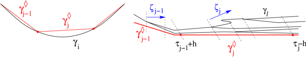
Figure 7: Left: approximating an $\varepsilon_{0}$-good path $\gamma_{i}$ in the irrigation plan $\chi$ with a polygonal $\gamma^{\diamondsuit}$. Right: the weight $W^{\diamondsuit}$ along the segment with endpoints $\gamma^{\diamondsuit}(\tau_{j-1}+h^{\prime})$, $\gamma^{\diamondsuit}(\tau_{j}-h^{\prime})$ is compared with the sum of weights along corresponding $\varepsilon_{n}$-good paths $\gamma_{l}^{\sharp}$ of $\chi_{n}$. Differently from the case illustrated in Fig. 6, we now compare weights at points having the same inner product with the vector $\zeta_{j}$, introduced at (5.18).

Toward a proof of Theorem 5.1, the heart of the matter is to achieve the inequalities (4.70)-(4.71) in steps 14-15. Since Lemma 4.5 no longer applies, a different argument must now be developed. The last three steps 14–16 in the proof of Theorem 4.1 can be replaced by the steps below. 14^′. We wish to compare the weights $W_{i}^{\diamondsuit}$ with a sum of the weights along the corresponding $\varepsilon_{n}$-good elementary paths in the approximating irrigation plans $\chi_{n}$. This will be done separately on each subinterval $[\tau_{j-1},\tau_{j}]$, where the tangent vector $\dot{\gamma}^{\diamondsuit}(t)=v_{j}$ is constant.

As in step 9 of the previous proof, in connection with $\gamma_{i}\Big{|}_{[\tau_{j-1},\tau_{j}]}$ we can determine a family $\Gamma_{i,j}$ of $\varepsilon_{n}$-good paths $\gamma_{\ell}:[a_{\ell},b_{\ell}]\mapsto\mathbb{R}^{d}$ in the irrigation plan $\chi_{n}$, which approach $\gamma_{i}$ as $n\to\infty$ (see Fig. 7, right). By construction, the corresponding weight and multiplicity functions $W_{\ell},m_{\ell}:[a_{\ell},b_{\ell}]\mapsto\mathbb{R}$ are non-increasing and satisfy

$${d\over ds}\bigl{[}W_{\ell}(s)-m_{\ell}(s)\bigr{]}~{}=~{}-f(\dot{\gamma}_{\ell}(s),W_{\ell}(s)).$$ (5.16)

As remarked in the previous sections, each elementary path $\gamma_{\ell}$ of $\chi_{n}$ is contained in some maximal path $\widehat{\gamma}_{q}:[a_{q},b_{q}]\mapsto\mathbb{R}^{d}$. The set of elementary paths is partially ordered by setting

$$\gamma_{\ell}~{}\prec~{}\gamma_{r}$$

if $\gamma_{\ell}$ and $\gamma_{r}$ are contained in the same maximal path, and $b_{\ell}\leq a_{r}$. The set of paths which bifurcate from the tip of $\gamma_{\ell}$ is defined as

$${\cal O}(\ell)~{}\doteq~{}\{r\,;~{}~{}\gamma_{\ell}~{}\prec~{}\gamma_{r}~{}~{}\hbox{and}~{}~{}b_{\ell}=a_{r}\}.$$

At the endpoint of $\gamma_{\ell}$, by construction we have

$$W_{\ell}(b_{\ell})-m_{\ell}(b_{\ell})~{}=~{}\sum_{r\in{\cal O}(\ell)}\bigl{[}W_{r}(a_{r})-m_{r}(a_{r})\bigr{]}.$$ (5.17)

Of course, the above definition here implies $a_{r}=b_{\ell}$. 15^′. Throughout this step we fix an elementary path $\gamma_{i}$ of the limit irrigation plan $\chi$. To shorten notation, we shall thus drop the index $i$ and simply write $\gamma^{\diamondsuit}=\gamma^{\diamondsuit}_{i}$, $W^{\diamondsuit}=W^{\diamondsuit}_{i}$, etc. To establish a comparison we observe that, by the convexity and positive homogeneity of the map $v\mapsto f\bigl{(}v,W^{\diamondsuit}(\tau_{j})\bigr{)}$, there exists a vector $\zeta_{j}\in\mathbb{R}^{d}$ such that

$$f(v_{j},W^{\diamondsuit}(\tau_{j}))~{}=~{}\langle v_{j},\zeta_{j}\rangle,\qquad\qquad f(v,W^{\diamondsuit}(\tau_{j}))~{}\geq~{}\langle v,\zeta_{j}\rangle\quad\hbox{for all}~{}v\in\mathbb{R}^{d}\,.$$ (5.18)

Notice that, if $f$ is smooth, then $\zeta_{j}=\nabla_{v}f\bigl{(}v_{j},W^{\diamondsuit}(\tau_{j})\bigr{)}$ is simply the gradient of $f$ w.r.t. the variable $v\in\mathbb{R}^{d}$. If $f$ is convex but not smooth, then $\zeta_{j}$ can be any sub-gradient.

By construction, for $t\in[\tau_{j-1},\tau_{j}]$ the derivative $\dot{\gamma}^{\diamondsuit}(t)=v_{j}$ is constant. From (5.14), using (5.10) and then (5.8)-(5.9) and (5.12), one obtains

$$\begin{array}[]{l}\displaystyle{d\over dt}\bigl{[}W^{\diamondsuit}(t)-m^{\diamondsuit}(t)\bigr{]}~{}\displaystyle=~{}-\tilde{f}(v_{j},W^{\diamondsuit}(t))\\[11.38109pt] \qquad\displaystyle\geq~{}-f\bigl{(}v_{j},W^{\diamondsuit}(\tau_{j})\bigr{)}+\delta_{0}-\kappa L|\tau_{j}-t|~{}\geq~{}-\langle v_{j},\zeta_{j}\rangle+{\delta_{0}\over 2}\,.\end{array}$$ (5.19)

Let $\gamma_{\ell}:[a_{\ell},\,b_{\ell}]\mapsto\mathbb{R}^{d}$ be any $\varepsilon_{n}$-good path in $\chi_{n}$. For $t\in[\tau_{j-1}+h,\tau_{j}-h]$ we define

$$s_{\ell}(t)~{}\doteq~{}\inf\Big{\{}s\geq a_{\ell}\,;~{}~{}\langle\zeta_{j},\gamma_{\ell}(s)\rangle\,\geq\,\big{\langle}\zeta_{j},\gamma^{\diamondsuit}(t)\big{\rangle}\Big{\}},$$ (5.20)

and consider the set of indices

$$I(t)~{}\doteq~{}\bigl{\{}\ell\,;~{}~{}a_{\ell}\,<\,s_{\ell}(t)\,<\,b_{\ell}\bigr{\}}.$$

By an approximation argument, we can assume that each $\gamma_{\ell}$ is a polygonal, with $\langle\dot{\gamma}_{\ell}(t),\zeta_{j}\rangle\not=0$ for a.e. $t\in[a_{\ell},b_{\ell}]$. This implies

$${d\over dt}s_{\ell}(t)~{}=~{}{\langle v_{j},\zeta_{j}\rangle\over\langle\dot{\gamma}_{\ell}(s_{\ell}(t)),\zeta_{j}\rangle}~{}>~{}0$$ (5.21)

for all except finitely many times $t$. We can now estimate

$$\begin{array}[]{l}\displaystyle{d\over dt}\sum_{\ell\in I(t)}\bigl{[}W_{\ell}(s_{\ell}(t))-m_{\ell}(s_{\ell}(t))\bigr{]}~{}=~{}\displaystyle-\sum_{\ell\in I(t)}{\langle v_{j},\zeta_{j}\rangle\over\langle\dot{\gamma}_{\ell}(s_{\ell}(t)),\zeta_{j}\rangle}\cdot f(\dot{\gamma}_{\ell}(s_{\ell}(t)),W_{\ell}(s_{\ell}(t)))\\[11.38109pt] \qquad\leq~{}\displaystyle-\sum_{\ell\in I(t)}\langle v_{j},\zeta_{j}\rangle\,{f(\dot{\gamma}_{\ell}(s_{\ell}(t)),W^{\diamondsuit}(\tau_{j}))\over\langle\dot{\gamma}_{\ell}(s_{\ell}(t)),\zeta_{j}\rangle}\cdot\min\left\{{W_{\ell}(s_{\ell}(t))\over W^{\diamondsuit}(\tau_{j})}\,,\,1\right\}\\[11.38109pt] \qquad\leq~{}\displaystyle-\sum_{\ell\in I(t)}\langle v_{j},\zeta_{j}\rangle\,\min\left\{{W_{\ell}(s_{\ell}(t))\over W^{\diamondsuit}(\tau_{j})}\,,\,1\right\}\,.\end{array}$$ (5.22)

Here the first identity follows from (5.4)-(5.5) and (5.21), while the second inequality is a consequence of (5.18) and of the concavity of the map $W\mapsto f(v,W)$. The third inequality follows from (5.18). Notice that, at points where two or more paths bifurcate, by (5.17) the sum $\sum_{\ell\in I(t)}[W_{\ell}(t)-m_{\ell}(t)]$ remains continuous. However, this sum will have downward jumps at points where one of the maps $t\mapsto s_{\ell}(t)$ is discontinuous. 16^′. We are now ready to describe the comparison argument that replaces the estimates in step 15 of the proof of Theorem 4.1. As in the previous proof, for each large $n$ we can identify a finite family of $\varepsilon_{n}$-good paths $\gamma_{\ell}$ in $\chi_{n}$ which converge to the elementary path $\gamma_{i}$ of $\chi$. In particular, for $n\geq 1$ large enough, we can assume

$$\sum_{\ell}m_{\ell}(s_{\ell}(t))~{}\geq~{}m^{\diamondsuit}(t)\qquad\qquad\hbox{for all}~{}t\in[\tau_{j-1}+h\,,~{}\tau_{j}-h],~{}~{}j=1,2,\ldots,m(i).$$ (5.23)

By backward induction, assume that

$$\bigl{[}W^{\diamondsuit}(\tau_{j}+h)-m^{\diamondsuit}(\tau_{j}+h)\bigr{]}~{}\leq~{}\sum_{\ell\in I(\tau_{j}+h)}\bigl{[}W_{\ell}(s_{\ell}(\tau_{j}+h))-m_{\ell}(s_{\ell}(\tau_{j}+h)\big{]}.$$ (5.24)

Since $\tilde{f}=0$ for $t\in[\tau_{j}-h,\tau_{j}+h]$ while all differences $W_{\ell}-m_{\ell}$ are non-increasing, this immediately yields

$$\bigl{[}W^{\diamondsuit}(\tau_{j}-h)-m^{\diamondsuit}(\tau_{j}-h)\bigr{]}~{}=~{}\bigl{[}W^{\diamondsuit}(\tau_{j}+h)-m^{\diamondsuit}(\tau_{j}+h)\bigr{]}~{}\leq~{}\sum_{\ell\in I(\tau_{j}-h)}\bigl{[}W_{\ell}(s_{\ell}(\tau_{j}-h))-m_{\ell}(s_{\ell}(\tau_{j}-h)\big{]}.$$ (5.25)

For $t\in[\tau_{j-1}+h\,,~{}\tau_{j}-h]$, we claim that the quantity

$$\Phi(t)~{}\doteq~{}\bigl{[}W^{\diamondsuit}(t)-m^{\diamondsuit}(t)\bigr{]}-\sum_{\ell\in I(t)}\bigl{[}W_{\ell}(s_{\ell}(t))-m_{\ell}(s_{\ell}(t))\bigr{]}$$

remains non-positive. Indeed, comparing the derivatives in (5.19) and (5.22) one obtains

$$\begin{array}[]{l}\displaystyle{d\over dt}\Phi(t)~{}\geq~{}\displaystyle-\langle v_{j},\zeta_{j}\rangle+{\delta_{0}\over 2}+\sum_{\ell\in I(t)}\langle v_{j},\zeta_{j}\rangle\,\min\left\{{W_{\ell}(s_{\ell}(t))\over W^{\diamondsuit}(\tau_{j})}\,,\,1\right\}.\end{array}$$ (5.26)

Set

$$t^{*}~{}\doteq~{}\sup\,\bigl{\{}t\leq\tau_{j}\,;~{}~{}\Phi(t)>0\bigr{\}}.$$

If $t^{*}>\tau_{j-1}+h$, to derive a contradiction we will show that

$${d\Phi\over dt}\bigg{|}_{t=t^{*}}~{}>~{}0.$$ (5.27)

Toward this goal we observe that, by continuity, $\Phi(t^{*})=0$. Since the map $t\mapsto W^{\diamondsuit}(t)$ is decreasing, by (5.23) we obtain

$$W^{\diamondsuit}(\tau_{j})-\sum_{\ell}W_{\ell}(s_{\ell}(t^{*}))~{}\leq~{}W^{\diamondsuit}(t^{*})-\sum_{\ell}W_{\ell}(s_{\ell}(t^{*}))~{}=~{}m^{\diamondsuit}(t^{*})-\sum_{\ell}m_{\ell}(s_{\ell}(t^{*}))~{}\leq~{}0.$$ (5.28)

By (5.26) this implies

$${d\Phi\over dt}\bigg{|}_{t=t^{*}}~{}\geq~{}\displaystyle-\langle v_{j},\zeta_{j}\rangle+{\delta_{0}\over 2}+\sum_{\ell\in I(t^{*})}\langle v_{j},\zeta_{j}\rangle\,\min\left\{{W_{\ell}(s_{\ell}(t^{*}))\over W^{\diamondsuit}(\tau_{j})}\,,\,1\right\}~{}\geq~{}{\delta_{0}\over 2}.$$ (5.29)

We thus conclude that $\Phi(t)\leq 0$ for all $t\geq\tau_{j-1}$. This achieves the key inductive step, showing that the inequality (5.24) remains valid with $j$ replaced by $j-1$.

The remainder of the proof follows the same arguments used for Theorem 4.1. MM     

Remark 5.2

By a minor modification of the previous arguments, the above results can be further extended to the case where $f=f(x,v,W)$ depends continuously also on the variable $x\in\mathbb{R}^{d}$.

6 Optimal weighted irrigation plans

Given a positive, bounded Radon measure $\mu$ on $\mathbb{R}^{d}$, we define

$${\cal I}^{W,\psi}(\mu)~{}\doteq~{}\inf_{\chi}{\cal E}^{W,\psi}(\chi).$$

where the infimum is taken over all irrigation plans for the measure $\mu$. Relying on the lower semicontinuity of the weighted irrigation cost, proved in Theorems 4.1 and 5.1, we can now prove the existence of an optimal irrigation plan.

Theorem 6.1

Let $\mu$ be a positive, bounded Radon measure on $\mathbb{R}^{d}$. Let $f$ satisfy the assumptions in (A3) while $\psi$ satisfies (A1). If $\mu$ admits an irrigation plan with bounded weighted cost, then there exists an irrigation plan with minimum weighted cost.

Proof. Let $M=\mu(\mathbb{R}^{d})$ and let $(\chi_{n})_{n\geq 1}$ be a minimizing sequence of irrigation plans for $\mu$, so that

$$\lim_{n\to\infty}~{}{\cal E}^{W,\psi}(\chi_{n})~{}=~{}{\cal I}^{W,\psi}(\mu).$$ (6.1)

Since $f\geq 0$, by construction the weights are larger than the corresponding multiplicities. Namely, for every $\xi,t$ and $n\geq 1$ one has $W_{n}(\xi,t)\geq m_{n}(\xi,t)$. Since the costs in (6.1) are bounded, we deduce

$$\int_{0}^{M}\int_{0}^{+\infty}|\dot{\chi}_{n}(\xi,t)|\,dt\,d\xi~{}\leq~{}C$$

for some constant $C$ and all $n\geq 1$.

By the sequential compactness of traffic plans (see for example Proposition 3.27 in [1]), we can extract a subsequence $(\chi_{n_{j}})_{j\geq 1}$ pointwise converging to an irrigation plan $\chi$. The lower semicontinuity result proved in Theorem 5.1 yields

$${\cal E}^{W,\psi}(\chi)~{}\leq~{}\liminf_{n\to\infty}~{}{\cal E}^{W,\psi}(\chi_{n})~{}=~{}{\cal I}^{W,\psi}(\mu).$$ (6.2)

Hence $\chi$ achieves the minimum weighted cost. MM     

We conclude by proving the lower semicontinuity of the weighted irrigation cost, w.r.t. weak convergence of measures.

Theorem 6.2

Let $f$ satisfy the assumptions in (A3) while $\psi$ satisfies (A1). Let $(\mu_{n})_{n\geq 1}$ be a sequence of bounded positive measures, with uniformly bounded supports, weakly converging to $\mu$. Then

$${\cal I}^{W,\psi}(\mu)~{}\leq~{}\liminf_{n\to\infty}{\cal I}^{W,\psi}(\mu_{n}).$$ (6.3)

Proof. Without loss of generality, one can assume

$$\liminf_{n\to\infty}~{}{\cal I}^{W,\psi}(\mu_{n})~{}\doteq~{}K~{}<~{}+\infty\,.$$ (6.4)

Let $\chi_{n}$ an optimal irrigation plan of $\mu_{n}$, so that ${\cal E}^{W,\psi}(\chi_{n})={\cal I}^{W,\psi}(\mu_{n})$ for every $n\geq 1$. As in the previous proof, by sequential compactness we can extract a subsequence $(\chi_{n_{j}})_{j\geq 1}$ pointwise converging to an irrigation plan $\chi$. A standard argument shows that $\chi$ provides an irrigation plan for the measure $\mu$. Using Theorem 4.1 we conclude

$${\cal I}^{W,\psi}(\mu)~{}\leq~{}{\cal E}^{W,\psi}(\chi)~{}\leq~{}\liminf_{n\to\infty}~{}{\cal E}^{W,\psi}(\chi_{n})~{}=~{}\liminf_{n\to\infty}{\cal I}^{W,\psi}(\mu_{n}).$$ (6.5)

MM     

Acknowledgment. This research was partially supported by NSF grant DMS-1714237, “Models of controlled biological growth”.

References

[1] M. Bernot, V. Caselles, and J. M. Morel,
Optimal transportation networks. Models and theory. Lecture Notes in Mathematics
1955, Springer, Berlin, 2009.
[2] M. Bernot, V. Caselles, and J. M. Morel,
Traffic plans.
Publicacions Matematiques49(2), (2005), 417–451.
[3] L. Brasco and F. Santambrogio,
An equivalent path functional formulation of branched transportation problems.
Discrete Contin. Dyn. Syst.29 (2011), 845–871.
[4] A. Bressan and Q. Sun,
On the optimal shape of tree roots and branches,
Math. Models & Methods Appl. Sci.28 (2018), 2763–2801
[5] A. Bressan, M. Palladino, and Q. Sun,
Variational problems for tree roots and branches,
submitted.
[6]
A. Bressan and F. Rampazzo,
On differential systems with vector-valued impulsive controls, Boll.
Un. Matematica Italiana2-B, (1988), 641-656.
[7]
E. N. Gilbert. Minimum cost communication networks.
Bell System Tech. J.46 (1967), 2209–2227.
[8] P. Hartman, Ordinary Differential Equations, Second Edition.
SIAM, 1982.
[9]
A. Kucia, Scorza Dragoni type theorems. Fund. Math.138 (1991), 197–203.
[10] F. Maddalena, J. M. Morel, and S. Solimini,
A variational model of irrigation patterns,
Interfaces Free Bound.5 (2003), 391–415.
[11] F. Maddalena and S. Solimini,
Synchronic and asynchronic descriptions of irrigation problems.
Adv. Nonlinear Stud.13 (2013), 583–623.
[12] A. Monteil,
Uniform estimates for a Modica-Mortola type approximation of branched transportation,
ESAIM Control Optim. Calc. Var.23 (2017), 309–335.
[13]
E. Oudet and F. Santambrogio,
A Modica-Mortola approximation for branched transport and applications.
Arch. Rational Mech. Anal.201 (2011), 115–142.
[14] P. Pegon, F. Santambrogio, and Q. Xia, A fractal shape optimization problem
in branched transport. J. Math. Pures Appl., to appear.
[15] R. Rishel,
An extended Pontryagin principle for control systems whose control laws contain measures.
SIAM J. Control3 (1965), 191–205.
[16]
F. Santambrogio,
Optimal channel networks, landscape function and branched transport.
Interfaces Free Bound.9 (2007), 149–169.
[17] F. Santambrogio, A Modica-Mortola approximation for branched transport.
C. R. Acad. Sci. Paris, Ser. I,
348 (2010) 941–945.
[18]
G. Scorza Dragoni,
Un teorema sulle funzioni continue rispetto ad una e misurabili rispetto ad un’altra variabile. (Italian)
Rend. Sem. Mat. Univ. Padova17 (1948), 102–106.
[19]
Q. Sun, Irrigable measures for weighted irrigation plans,
to appear.
[20]
Q. Xia, Optimal paths related to transport problems,
Comm. Contemp. Math.5 (2003), 251–279.
[21] Q. Xia,
Motivations, ideas and applications of ramified optimal transportation.
ESAIM Math. Model. Numer. Anal.49 (2015), 1791–1832.