T-Branes and $G_{2}$ Backgrounds

Abstract

Compactification of M- / string theory on manifolds with $G_{2}$ structure yields a wide variety of 4D and 3D physical theories. We analyze the local geometry of such compactifications as captured by a gauge theory obtained from a three-manifold of ADE singularities. Generic gauge theory solutions include a non-trivial gauge field flux as well as normal deformations to the three-manifold captured by non-commuting matrix coordinates, a signal of T-brane phenomena. Solutions of the 3D gauge theory on a three-manifold are given by a deformation of the Hitchin system on a marked Riemann surface which is fibered over an interval. We present explicit examples of such backgrounds as well as the profile of the corresponding zero modes for localized chiral matter. We also provide a purely algebraic prescription for characterizing localized matter for such T-brane configurations. The geometric interpretation of this gauge theory description provides a generalization of twisted connected sums with codimension seven singularities at localized regions of the geometry. It also indicates that geometric codimension six singularities can sometimes support 4D chiral matter due to physical structure “hidden” in T-branes.

UPR-1298-T

1 Introduction

Manifolds of special holonomy are of great importance in connecting the higher-dimensional spacetime predicted by string theory to lower-dimensional physical phenomena. This is because such manifolds admit covariantly constant spinors, thus allowing the macroscopic dimensions to preserve some amount of supersymmetry.

Historically, the most widely studied class of examples has centered on type II and heterotic strings compactified on Calabi–Yau threefolds [1]. This leads to 4D vacua with eight and four real supercharges, respectively. Such threefolds also play a prominent role in the study of F-theory and M-theory backgrounds, leading respectively to 6D and 5D vacua with eight real supercharges. Compactifications on Calabi–Yau spaces of other dimensions lead to a rich class of geometries, and correspondingly many novel physical systems in the macroscopic dimensions. In all these cases, the holomorphic geometry of the Calabi–Yau allows techniques from algebraic geometry to be used.

There are, however, other manifolds of special holonomy, most notably those with $G_{2}$ and $Spin(7)$ structure. For example, compactification of M-theory on $G_{2}$ and $Spin(7)$ spaces provides a method for generating a broad class of 4D and 3D $\mathcal{N}=1$ vacua, respectively.

Despite these attractive features, it has also proven notoriously difficult to generate singular compact geometries of direct relevance for physics. In the case of M-theory on a $G_{2}$ background, realizing a non-abelian ADE gauge group requires a three-manifold of ADE singularities (i.e., codimension four), and realizing 4D chiral matter requires codimension seven singularities. While there are now some techniques available to realize $G_{2}$ backgrounds with codimension four singularities, it is not entirely clear whether a smooth compact $G_{2}$ can be continuously deformed to such singular geometries, as necessary for physics.

Once one is given a codimension four ADE singularity, further degenerations at points of the three-manifold should produce the codimension seven singularities required for 4D chiral matter. It is expected that some of the fibers in the deformation family of [9] could acquire such point-like singularities, and we refer to that paper for a discussion on how that could be achieved from a geometric perspective.

In this approach to singular $G_{2}$ compactifications, rather than building the global geometry directly, the crucial idea is to use a dual gauge-theoretic description to characterize the appearance of such codimension seven singularities. In reference [23], the partial topological twist of a six-brane wrapped on a three-manifold $M$ embedded in a $G_{2}$ manifold was studied in some detail, and we shall refer to it as the “Pantev–Wijnholt” (PW) system. The choice of 4D vacuum is dictated in the six-brane gauge theory by an adjoint-valued one-form and a vector bundle. The eigenvalues of this one-form parameterize normal deformations in the local geometry $T^{\ast}M$, and this leads to a natural spectral cover description. Localized matter in this setup is obtained by allowing the one-form to vanish at various locations. In [23] this was used to analyze codimension seven singularities, and in reference [24] this analysis was greatly developed and also extended to the case of codimension six singularities, i.e. non-chiral matter. As argued in [24] a potentially appealing feature of these codimension six singularities is that they provide a way to possibly connect to one of the (few) methods available for building $G_{2}$ manifolds via twisted connected sums, using Calabi–Yau threefolds as building blocks [25, 26, 27]. The physics of M-theory compactified on such compact TCS $G_{2}$ manifolds has been studied in [28, 29, 30, 31, 32, 33, 34, 35, 36, 37, 24].

In the TCS construction of $G_{2}$ backgrounds [25, 27], one first begins with a pair $(M_{1},M_{2})$ of $G_{2}$-manifolds of the form $M_{i}=X_{i}\times S^{1}_{i,\text{ext}}$, where $S^{1}_{i,\text{ext}}$ is a circle we call “external” and $X_{i}$ is an asymptotically cylindrical Calabi–Yau threefold. This means that outside of a compact region, the Calabi–Yau metric looks like a $K3$ surface times a cylinder: $X_{i}\stackrel{{\scriptstyle\text{asymp.}}}{{\cong}}K3_{i}\times\mathbb{R}\times S^{1}_{i,\text{int}}$. One then glues $S^{1}_{1,\text{ext}}$ and $S^{1}_{2,\text{int}}$ using a hyperkähler rotation (and similarly for the other two circles) and shows that the resulting compact smooth manifold admits a full $G_{2}$ metric. Although all known examples result in smooth total spaces, it is reasonable to expect that degenerations in the Calabi–Yau building blocks will provide a way to generate the long sought for codimension six and seven singularities in compact models.

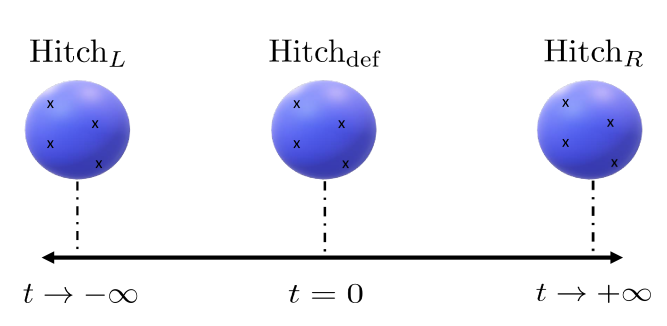
Figure 1: The local $G_{2}$ background of a three-manifold of ADE singularities is characterized by gauge theory on a three-manifold with corresponding ADE gauge group. In a local patch, this can be described by a Riemann surface $\Sigma$ with marked points fibered over an interval. In a suitable scaling limit of the metric, this can be viewed as a deformation of the Hitchin system over $\Sigma$ which asymptotes to solutions to the Hitchin system. See figure 2 for a depiction of the geometry associated with this local gauge theory.

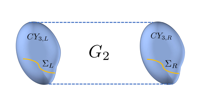
Figure 2: The local gauge theory analysis allows us to build up local $G_{2}$ backgrounds which asymptote to Calabi–Yau threefolds at two boundaries. The local $G_{2}$ background includes a three-manifold which is itself a Riemann surface $\Sigma$ fibered over an interval. This Riemann surface embeds in the boundary Calabi–Yau spaces. See figure 1 for a depiction of the asymptotic behavior of the gauge theory on the three-manifold as a deformation of the Hitchin system on $\Sigma$.

From this perspective, one might ask whether this is the most general starting point one can entertain for realizing localized matter in $G_{2}$ compactifications. One important clue comes from the structure of local $G_{2}$ backgrounds in the presence of non-zero fluxes. This leads to manifolds with structure group $G_{2}$, and these solutions can often be interpreted in terms of a system of lower-dimensional branes localized on subspaces inside the bulk geometry [38, 39, 40]. It is thus natural to ask about fluxed solutions with lower-dimensional defects.

In this paper we consider the case of non-abelian fluxes of a six-brane wrapped on a three-manifold. To accomplish this, we return to the local gauge theory on a six-brane (see also [41, 42, 24]). To date, most analyses of localized matter have assumed that the adjoint valued one-form is diagonal, and that there are no fluxes present in the three-manifold. Here, we shall relax this assumption and attempt to study a far broader class of situations. This necessarily means that the components of this one-form will not commute. We shall refer to this as a T-brane configuration (even though the matrix components are not upper triangular) since it naturally fits in the broader scheme of T-brane like phenomena. For earlier work on T-branes, see references [43, 44, 45, 46, 47, 48, 49, 50, 51, 52, 53, 54, 55, 56, 57, 58, 59, 60, 61, 62, 63].

Locally modelling the three-manifold as a Riemann surface fibered over an interval, we show that for each smooth fiber, the gauge theory on the Riemann surface is described by a mild deformation of Hitchin’s system on a complex curve (see figure 1). Since the local Hitchin system directly describes a local Calabi–Yau geometry (see e.g. [64, 11, 12, 48, 55]), we obtain a local deformation of a TCS-like construction which can be interpreted as building up a local $G_{2}$ background (see figure 2).

An important feature of these structures is the appearance of holomorphic geometry as a guide in constructing these local $G_{2}$ backgrounds. This points the way to a method for constructing $G_{2}$ backgrounds using more general holomorphic building blocks than those appearing in the classical TCS construction.

Another feature we study in great detail is the resulting localized matter obtained from such T-brane configurations. We provide examples where we explicitly determine the profile of localized matter fields in a given background. This involves solving a second order differential equation. We also develop algebraic methods for reading off the appearance of localized zero modes by determining the local ring structure of trapped matter. This is similar in spirit to the analysis of localized zero modes in T-brane configurations carried out in references [45, 46].

One of the outcomes of this analysis is that it also provides evidence for the existence of localized matter field configurations which would be “invisible” to the bulk $G_{2}$ geometry since they originate from degenerate spectral equations. Instead, they would be fully characterized by allow limiting behavior in the four-form $G$-flux of the M-theory background. We present explicit examples exhibiting this behavior. A canonical example is the “standard embedding” namely we embed the spin connection in the gauge bundle, taking our holomorphic vector bundle to be the tangent bundle on $T^{\ast}M$ dimensionally reduced (after a Fourier-Mukai transform / formally three T-dualities) to the three-manifold. Related examples show up in a number of other T-brane constructions (see e.g. [43, 48]).

The rest of this paper is organized as follows. We begin in section 2 by discussing the PW system, and its relation to geometric engineering. Next, in section 3 we show how to build examples of solutions to the PW system in cases with non-zero gauge field flux. In section 4 we present some general methods for analyzing zero modes in such backgrounds, and then proceed to determine the localized matter field wave functions by explicitly solving the corresponding partial differential equations. Section 5 presents a conjectural proposal for how to algebraically determine the localized zero mode content in fluxed solutions. We present our conclusions in section 6.

2 Six-Brane Gauge Theory on a Three-Manifold

In this section we discuss the gauge theory of a six-brane wrapped on a three-manifold, as obtained from M-theory on a $G_{2}$ background. Geometrically, we engineer this gauge theory from a three-manifold of ADE singularities with corresponding ADE gauge group - i.e., the local $G_{2}$ is a fibration of ADE singularities over a three-manifold. The terminology follows from the fact that the “brane” in question is actually a seven-dimensional supersymmetric gauge theory wrapped on the three-manifold, namely a six-brane. Supersymmetry is preserved since we assume the three-manifold is an associative three-cycle of the local $G_{2}$ manifold. It is also in accord with the type IIA string theory description of D6-branes wrapped on special Lagrangian submanifolds of a Calabi–Yau threefold. For a recent pedagogical discussion of geometric engineering, and the relation between localized gauge theories and singular geometry in the context of string compactification, see the online lectures of reference [66].

In terms of the geometry of the local $G_{2}$ background, we note that we have an associative three-form $\rho$ which pairs with the three-form potential $C$ of M-theory to form the complex moduli $C+i\rho$. Resolving the ADE fibers and performing a corresponding reduction to the three-manifold, we have a decomposition:

$$C=A_{\alpha}\wedge\omega^{\alpha}\text{, \ \ }\rho=\phi_{\alpha}\wedge\omega^{\alpha}$$ (2.1)

where the $\omega^{\alpha}$ are harmonic representatives of $(1,1)$ forms on the resolution of the local ADE singularity, and the $A_{\alpha}$ and $\phi_{\alpha}$ are one-forms on the three-manifold. Moreover $\alpha=1,\dots,r$ with $r$ being the rank of the ADE gauge group. One should think of this index as labeling the generators of the Cartan subalgebra of the corresponding ADE gauge group. The remaining generators are obtained from M2-branes wrapped on collapsing two-cycles of the fiber.

As explained in reference [23] (see also [41, 24, 67, 68]), the partial twist of a six-brane with gauge group $G$ on a three-manifold $M$ retains 4D $\mathcal{N}=1$ supersymmetry in the uncompactified directions. After the twist both the gauge field $A$ and $\phi$ become adjoint-valued one-forms on $M$. They combine into a complexified connection which we write as:

$$\mathcal{A}=A+i\phi,$$ (2.2)

which should be thought of as the bosonic component of a collection of 4D $\mathcal{N}=1$ chiral superfields which transform as a one-form on the three manifold. In our conventions, we take anti-hermitian generators for the Lie algebra so that $A^{{\dagger}}=-A$ and $\phi^{{\dagger}}=-\phi$. We shall also find it convenient to absorb the factor of $i$ to define a hermitian Higgs field:

$$\Phi\equiv i\phi.$$ (2.3)

We construct various curvatures from the complexified connection $D_{\mathcal{A}}$, its conjugate $D_{\overline{\mathcal{A}}}$ as obtained from $\overline{\mathcal{A}}=A-i\phi$ as well the purely real $D_{A}$. In a unitary gauge, we have $\mathcal{A}^{{\dagger}}=-\overline{\mathcal{A}}$. Locally these connections may be written as:

$$D_{\mathcal{A}}=d+\mathcal{A}\text{, \ \ }D_{\overline{\mathcal{A}}}=d+\overline{\mathcal{A}}\text{, \ \ }D_{A}=d+A.$$ (2.4)

We introduce gauge field strengths:

$$\mathcal{F}=\left[D_{\mathcal{A}},D_{\mathcal{A}}\right]\text{, \ \ }\mathcal{D}=\left[D_{\mathcal{A}},D_{\overline{\mathcal{A}}}\right]\text{, \ \ }F=\left[D_{A},D_{A}\right].$$ (2.5)

Once written in components the various field strengths are:

$$\mathcal{F}_{ij} =\partial_{i}\mathcal{A}_{j}-\partial_{j}\mathcal{A}_{i}+\left[\mathcal{A}_{i},\mathcal{A}_{j}\right]$$ (2.6)

$$\mathcal{D}_{ij} =\partial_{i}\overline{\mathcal{A}}_{j}-\partial_{j}\mathcal{A}_{i}+\left[\mathcal{A}_{i},\overline{\mathcal{A}}_{j}\right]$$ (2.7)

$$F_{ij} =\partial_{i}A_{j}-\partial_{j}A_{i}+\left[A_{i},A_{j}\right].$$ (2.8)

In terms of the original fields $A$ and $\phi$, the complexified field strengths decompose as:

$$\operatorname{Im}\mathcal{F}_{ij} =F_{ij}-[\phi_{i},\phi_{j}]$$ (2.9)

$$\operatorname{Re}\mathcal{F}_{ij} =(\partial_{i}+A_{i})\cdot\phi_{j}-(\partial_{j}+A_{j})\cdot\phi_{i}$$ (2.10)

$$\operatorname{Re}\mathcal{D}_{ij} =-(\partial_{i}+A_{i})\cdot\phi_{j}-(\partial_{j}+A_{j})\cdot\phi_{i}$$ (2.11)

$$\operatorname{Im}\mathcal{D}_{ij} =F_{ij}+[\phi_{i},\phi_{j}].$$ (2.12)

We are considering here the equations for the fields supported on the three-manifold, and thus the the indices $i,j$ run from $1$ to $3$. Variation of the 7D gaugino produces the corresponding conditions to have a 4D $\mathcal{N}=1$ supersymmetric vacuum. These are conveniently packaged as F-terms and D-terms, which are respectively metric independent and dependent:

$$\mathcal{F}_{ij}=0\text{ \ \ and \ \ }g^{ij}\mathcal{D}_{ij}=0,$$ (2.13)

in the obvious notation. The moduli space of vacua is then given by two equivalent presentations:

$$\{\mathcal{F} =0\}/G_{\mathbb{C}}^{\text{gauge}}$$ (2.14)

$$\{\mathcal{F} =0\text{, \ \ }g^{ij}\mathcal{D}_{ij}=0\}/G_{U}^{\text{gauge}}\text{,}$$ (2.15)

where here, $G_{\mathbb{C}}^{\text{gauge}}$ refers to complexified gauge transformations and $G_{U}^{\text{gauge}}$ refers to unitary gauge transformations. We refer to both presentations of the moduli space as the defining equations of the Pantev–Wijnholt (PW) system.

The F-term equations of motion are obtained from the critical points of the Chern-Simons superpotential for the complexified connection:

$$\mathcal{W}\left[\mathcal{A}\right]=\frac{s}{4\pi}\int_{M}\text{Tr}_{\mathfrak{g}_{\mathbb{C}}}\left(\mathcal{A\wedge}d\mathcal{A+}\frac{2}{3}\mathcal{A\wedge A\wedge A}\right),$$ (2.16)

for $s$ a complex parameter. Four-dimensional $\mathcal{N}=1$ vacua are labelled by critical points of $\mathcal{W}$ modulo $G_{\mathbb{C}}^{\text{gauge}}$.

More precisely, in the description specified by F-terms modulo $G_{\mathbb{C}}^{\text{gauge}}$ gauge transformations, the appropriate notion of “stability” is that we only look at connections with semisimple monodromy. By the Donaldson–Corlette theorem [70, 71], these automatically solve the harmonic metric equation, i.e. the D-term. An interesting feature is that for any hermitian generator of the algebra, the signature of the real matrix $\mathcal{D}_{ij}^{B}$ (with $B$ an index in the adjoint) must have at least one $+$ sign and one $-$ sign each. This is simply to satisfy the D-term constraint. We note that this is in accord with the “Hessian condition” of references [23, 24] observed in the special case where the adjoint-valued one-form is diagonal. In this case, the eigenvalues must have, in some basis, signature $(+,+,-)$ or $(-,-,+)$. The vanishing locus of the Higgs field then specifies a chiral or anti-chiral zero mode.

Another way to study this system is to first consider stable holomorphic vector bundles on the local Calabi–Yau $T^{\ast}M\equiv X$. These are described by Hermitian–Yang–Mills (HYM) instantons [72, 73]. Taking the linearization of the HYM equations in a neighborhood of the zero section $M$ then produces the same equations [23]. Briefly summarizing this approach, we introduce a $(0,1)$ connection:

$$\overline{\partial}_{\mathbb{A}}=\overline{\partial}+\mathbb{A}\text{.}$$ (2.17)

The conditions to have a stable holomorphic vector bundle are a F-term and a D-term:

$$\mathbb{F}_{(0,2)}=0\text{ \ \ and \ \ }J\wedge J\wedge\mathbb{F}_{(1,1)}=0\text{,}$$ (2.18)

with $J$ the Kähler form on $X$. To make contact with the PW equations, we consider $\mathbb{A}$ as a complexified gauge field which splits up as:

$$\mathbb{A}=A_{i}dx^{i}+\phi_{j}dp^{j},$$ (2.19)

where $x$ are local coordinates on $M$ and $p$ are local coordinates in the cotangent direction. The topological twist amounts to making a further identification $dp^{i}=J_{j}^{i}dx^{j}$ which introduces an additional factor of $\sqrt{-1}$ thus recovering (2.2). A helpful feature of this construction is that it also describes the heterotic dual to this local model. More precisely, it is the linearization obtained from a (singular) $T^{3}$ fibration over $M$.

This alternate presentation already points to an important general point: A priori, there is no reason for the components $\phi_{j}$ in equation (2.19) to be simultaneously diagonalizable. Returning to the PW equations, this also means there is no reason to exclude gauge fluxes through the three-manifold. Let us also note that even if such fluxes are present, it does not directly mean there will be a bulk four-form flux in the $G_{2}$ model. This is because these fluxes are inherently localized on the three-manifold and are “hard to see” from the bulk point of view. Indeed, the local geometry of the $G_{2}$ background is primarily sensitive to just the eigenvalues of $\phi_{i}$ and bulk $G-$fluxes, and not to any of these non-abelian local features.

A canonical example is the tangent bundle of $T^{\ast}M$. It has the important feature that the spectral cover description is degenerate. On the three manifold $M$ we have a vector bundle with $SU(3)$ structure group and the $\phi$’s certainly do not commute. Let us note that in heterotic / F-theory duality, the standard embedding also corresponds to a T-brane configuration of an F-theory compactification [43, 48].

3 Fluxed PW Solutions

In this section we consider fluxed solutions of the PW system. Our strategy for obtaining such configurations will be to consider a local description of the three-manifold as a Riemann surface fibered over an interval, and we shall often further specialize to the case of a Cartesian product $M=\Sigma\times I$ with $\Sigma$ a Riemann surface and $I$ an interval. This description will only be valid locally, and so we can either assume these solutions extend outside of the patch in question, or alternatively, we can cut off the solution by allowing singular field configurations at prescribed regions of the three manifold.

To aid in our study of fluxed PW solutions, we shall often assume the metric on the three-manifold takes the form:

$$ds_{M}^{2}=g_{tt}dt^{2}+g_{ab}dx^{a}dx^{b},$$ (3.1)

where in the above, $t$ denotes a local coordinate on $I$, and $x^{a}$ for $a=1,2$ denote coordinates on the Riemann surface, and since we often focus on metric independent questions, we shall also sometimes take the metric to be flat in some local patch.

In terms of this presentation, the PW equations take the form:

$$F_{ab}-[\phi_{a},\phi_{b}] =0\,,$$ (3.2)

$$D_{a}\phi_{b}-D_{b}\phi_{a} =0\,,$$ (3.3)

$$g^{ab}D_{a}\phi_{b}+g^{tt}D_{t}\phi_{t} =0\,,$$ (3.4)

$$F_{ta}-[\phi_{t},\phi_{a}] =0\,,$$ (3.5)

$$D_{t}\phi_{a}-D_{a}\phi_{t} =0\,,$$ (3.6)

modulo unitary gauge transformations. In the above, we have written $D_{i}=\partial_{i}+A_{i}$ for the covariant derivative. We now observe that the first three equations describe a small deformation of the standard Hitchin system of reference [74]. Indeed, introducing a covariant derivative $D_{\Sigma}=d+A_{\Sigma}$ and a one-form $\phi_{\Sigma}$ on each fiber, we have:

$$F_{\Sigma}-[\phi_{\Sigma},\phi_{\Sigma}] =0\,,$$ (3.7)

$$D_{\Sigma}\phi_{\Sigma} =0\,,$$ (3.8)

$$\ast_{\Sigma}\,D_{\Sigma}\ast_{\Sigma}\phi_{\Sigma} =-g^{tt}D_{t}\phi_{t}\,,$$ (3.9)

which would have described the Hitchin system in the special case where $g^{tt}D_{t}\phi_{t}=0$.

We remark that these equations tell us that the induced Hitchin system does not describe a Higgs bundle in the mathematician’s sense [75]; indeed, the condition for harmonicity of the bundle metric is [70, 71] $D_{\Sigma}\ast_{\Sigma}\phi_{\Sigma}=0$, and equation (3.9) tells us that a PW solutions gives a deformation of that condition along the $t$-direction. We point out that the dependence of equation (3.9) on the bundle metric is hidden in the definition of the Hodge star $\ast$.

The remaining F-term relations $\mathcal{F}_{ta}=0$ can also be interpreted as a flow equation:

$$\mathcal{F}_{ta}=\partial_{t}\mathcal{A}_{a}-\partial_{a}\mathcal{A}_{t}+\left[\mathcal{A}_{t},\mathcal{A}_{a}\right]=0$$ (3.10)

i.e.:

$$\partial_{t}\mathcal{A}_{a}+\left[\mathcal{A}_{t},\mathcal{A}_{a}\right]=\partial_{a}\mathcal{A}_{t}.$$ (3.11)

Geometrically, we interpret the flow equations as a gluing construction for local Calabi–Yau threefolds. To see why, we first recall the correspondence between the Hitchin system on a genus $g$ curve $\Sigma$ and the integrable system associated to a family of non-compact Calabi–Yau manifolds each containing $\Sigma$ as a curve of ADE singularities [12, 11, 55]. Let $Y$ denote the Calabi–Yau threefold that is the central fiber of the deformation family. Recall that the isomorphism between the integrable systems implies in particular that variations in the complex structure for $Y$ are described by (spectral curves of) Higgs fields $\varphi$ - i.e., adjoint-valued $(1,0)$-forms on the curve $\Sigma$. With notation as in equation (2.1) for harmonic $(1,1)$ forms on the ADE singularity, the variations of the holomorphic three-form on the local Calabi–Yau decompose as:

$$\delta\Omega_{(2,1)}=\varphi_{\alpha}\wedge\omega^{\alpha}\text{.}$$ (3.12)

The Calabi–Yau condition enforces the condition $\overline{\partial}(\delta\Omega_{(2,1)})=0$, which translates to one of the Hitchin equations:

$$\overline{\partial}_{A}\varphi=0\text{.}$$ (3.13)

The deformation of line (3.9) tells us that the righthand side is no longer zero. Translating back to the Calabi–Yau integrable system, we see that we instead get a deformation of a Calabi–Yau manifold that does not respect the Kähler condition, resulting in a “symplectic Calabi–Yau” in the sense of Smith, Thomas and Yau [76] (for a recent discussion see reference [77], and for a review see reference [78] and additional references therein).

From the perspective of the local $G_{2}$, we thus see that asymptotically near the boundaries of the interval, we retain an approximate Calabi–Yau geometry, but as we proceed to the interior of the interval, each fiber will instead be described by a symplectic Calabi–Yau.

Let us illustrate the correspondence between the spectral equation for the Higgs field and deformations of its dual local Calabi–Yau in the case of $G=SU(N)$. The spectral equation in the fundamental representation is:

$$\det(u_{\text{hol}}\mathbb{I}_{N}-\varphi_{\text{hol}})=0,$$ (3.14)

with $u_{\text{hol}}$ a local coordinate in the cotangent direction of $T^{\ast}\Sigma$. Since we also have a Higgs field in the more general case, it is natural to consider two related spectral equations, as generated by the PW system. First, we have the one closely linked to the asymptotic Hitchin system associated with $\Phi=i\phi$:

$$\det(u_{z}\mathbb{I}_{N}-\Phi_{z})=0.$$ (3.15)

This equation only makes sense asymptotically, since in the bulk of the three-manifold, the Higgs field of the PW system is not a holomorphic (or even meromorphic) section of a bundle on the curve $\Sigma$. Indeed, more generally we ought to speak of the spectral equations:

$$\det(u_{i}\mathbb{I}_{N}-\Phi_{i})=0.$$ (3.16)

where here, $u_{i}$ for $i=1,2,3$ are coordinates in the cotangent direction of $T^{\ast}M$. This is a triplet of real equations in $T^{\ast}M$ which cut out a three-manifold in this ambient space. Geometrically, then, we can interpret the spectral equation of line (3.16) as a special Lagrangian manifold in $T^{\ast}M$ with boundaries specified by the holomorphic curves dictated by equation (3.15). Indeed, the PW equations ensure that supersymmetry has been preserved.

This also allows us to elaborate on the sense in which having $[\Phi_{i},\Phi_{j}]\neq 0$ is an example of T-brane phenomena. Even though each $\Phi$ takes values in the unitary Lie algebra $\mathfrak{g}$, it is also natural to consider linear combinations which take values in the complexification $\mathfrak{g}_{\mathbb{C}}$. If the complexified combination $\Phi_{z}=\Phi_{1}+i\Phi_{2}$ is a nilpotent element of $\mathfrak{g}_{\mathbb{C}}$, then we observe that the holomorphic spectral equation of line (3.15) is degenerate. Indeed, even though $\Phi_{1}$ and $\Phi_{2}$ are hermitian (and thus never nilpotent), their complex combination can of course be nilpotent. From the perspective of a global $G_{2}$ background, this also suggests that such phenomena may be invisible to the geometry, instead being encoded in non-abelian degrees of freedom localized along lower-dimensional subspaces. A related comment is that even though each component of the Higgs field $\Phi$ is hermitian, when these matrices do not commute, there is no canonical way in which we can speak of the spectral sheets intersecting along a locus of symmetry enhancement. We return to these issues in section 5.

The plan in the remainder of this section is as follows. First, we discuss some general aspects of background solutions in a local patch. Starting from a solution along a single fiber, we show that this solution extends to a local neighborhood of the three-manifold. We then present some explicit examples of backgrounds, including T-brane configurations.

3.1 Background Solutions in a Local Patch

We first locally characterize solutions of the system in a patch with trivial topology. By abuse of notation, we continue to write $M$ for this local patch. The F-term equations of motion tell us that we are dealing with a complexified flat connection, so the most general solution for the gauge connection is of the form:

$$\mathcal{A}=g^{-1}dg,$$ (3.17)

where $g:M\rightarrow G_{\mathbb{C}}$ takes values in the complexified gauge group. One must remember that here, we are working with a complexified connection, so even though the gauge field appears to be “pure gauge,” we must only permit gauge transformations which do not alter the asymptotic behavior of the gauge field. A related point is that to actually find a solution in unitary gauge, we need to substitute our expression for $\mathcal{A}=g^{-1}dg$ into the D-term constraint $g^{ij}D_{i}\phi_{j}=0$, resulting in a second order partial differential equation for $g(x)$.

As an illustrative example, suppose that $g$ is of the form:

$$W\cdot g=1+h+\frac{h^{2}}{2!}+...,$$ (3.18)

where $W$ is a general element of $G_{\mathbb{C}}$, and we have introduced an infinitesimal $h:M\rightarrow\mathfrak{g}_{\mathbb{C}}$ a Lie algebra valued function on the patch. Then, the complexified connection takes the form:

$$\mathcal{A}=dh+...\text{.}$$ (3.19)

Feeding this into the D-term constraint, we get, to leading order in $h$:

$$g^{ij}\mathcal{D}_{ij}=g^{ij}\partial_{i}\partial_{j}(h-h^{{\dagger}})=0.$$ (3.20)

So in other words, $\operatorname{Im}h$ is a Lie algebra valued harmonic map.

There are, of course, more general choices for $g(x)$ and we will in fact find it necessary to consider a more general choice of complexified connection to generate novel examples of T-brane configurations with localized matter.

3.2 Power Series Solutions

We now turn to a more systematic method for building up solutions of the PW equations in the presence of flux. The basic idea is that we shall split up our three-manifold as a local product $\Sigma\times I$ with $\Sigma$ a Riemann surface (possibly with punctures) and $I$ an interval. We introduce a local coordinate on $I$ denoted by $t$ so that $t=0$ is in the interior of the interval, and coordinates $x_{a}$ for $a=1,2$ for coordinates on the Riemann surface. It will sometimes prove convenient to also use coordinates $z=x_{1}+ix_{2}=x+iy$.

We show that if enough initial data is specified at $t=0$, then we can start to extend this solution in a neighborhood, building up a solution on the entire patch of the three-manifold. The demonstration of this will be to develop a power series expansion in the variable $t$ for all fields of the PW system, and solve the expanded equations order by order in this parameter. We shall not concern ourselves with whether the series converges, because we do actually anticipate that there could be singular behavior for the fields at locations on the three-manifold. This is additional physical data, and must be allowed to make sense of the most general configurations of relevance for physics. As a final comment, while we cannot exclude the possibility of solutions which do not admit a power series expansion in some local neighborhood, we expect on physical grounds that such solutions are likely pathological as they would significantly a breakdown of the $G_{2}$ structure at more than just a higher codimension subspace.

We consider a series expansion of the complexified connection around $t=0$,

$$\mathcal{A}_{i}(t,x_{a})=\sum_{j=0}^{\infty}\mathcal{A}_{i}^{(j)}(x_{a})t^{j}\,.$$ (3.21)

Furthermore, it is convenient to work in “temporal gauge” with:

$$A_{t}^{(j)}=0\,.$$ (3.22)

In this gauge, and with the power series expansion (3.21), the PW equations can be written as non-trivial differential equations on the coefficients

$$\begin{gathered}\sum_{j=0}^{\infty}\left(\partial_{a}A_{b}^{(j)}-\partial_{b}A_{a}^{(j)}+\sum_{m=0}^{j}\left([A_{a}^{(j-m)},A_{b}^{(m)}]-[\phi_{a}^{(j-m)},\phi_{b}^{(m)}]\right)\right)t^{j}=0\cr\sum_{j=0}^{\infty}\left(\partial_{a}\phi_{b}^{(j)}+\sum_{m=0}^{j}[A_{a}^{(j-m)},\phi_{b}^{(m)}]-\partial_{b}\phi_{a}^{(j)}-\sum_{m=0}^{j}[A_{b}^{(j-m)},\phi_{a}^{(m)}]\right)t^{j}=0\,,\end{gathered}$$ (3.23)

together with equations which fix the higher order coefficients in terms of the preceding ones,

$$\begin{gathered}\sum_{j=0}^{\infty}\left(g^{ab}\left(\partial_{a}\phi_{b}^{(j)}+\sum_{m=0}^{j}[A_{a}^{(j-m)},\phi_{b}^{(m)}]\right)+(j+1)g^{tt}\phi_{t}^{(j+1)}\right)t^{j}=0\cr\sum_{j=0}^{\infty}\left((j+1)A_{a}^{(j+1)}-\sum_{m=0}^{j}[\phi_{t}^{(j-m)},\phi_{a}^{(m)}]\right)t^{j}=0\cr\sum_{j=0}^{\infty}\left((j+1)\phi_{a}^{(j+1)}-\partial_{a}\phi_{t}^{(j)}-\sum_{m=0}^{j}[A_{a}^{(j-m)},\phi_{t}^{(m)}]\right)t^{j}=0\,.\end{gathered}$$ (3.24)

At $t=0$ these equations collapse to

$$\begin{gathered}F_{ab}^{(0)}-[\phi_{a}^{(0)},\phi_{b}^{(0)}]=0\cr D_{a}^{(0)}\phi_{b}^{(0)}-D_{b}^{(0)}\phi_{a}^{(0)}=0\cr g^{ab}D_{a}^{(0)}\phi_{b}^{(0)}+g^{tt}\phi_{t}^{(1)}=0\cr A_{a}^{(1)}-[\phi_{t}^{(0)},\phi_{a}^{(0)}]=0\cr\phi_{a}^{(1)}-D_{a}^{(0)}\phi_{t}^{(0)}=0\,.\end{gathered}$$ (3.25)

We will assume that $A_{a}^{(0)}$ and $\phi_{a}^{(0)}$ are such that the non-trivial zeroth order differential equations are solved, and the higher order coefficients are fixed by solving the linear equations. The one remaining free parameter is $\phi_{t}^{(0)}$, which sets the “trajectory” of the solution. Once we are given this initial set of data, solving the zeroth order equations, we can show that the PW equations are solved to all orders in $t$.

To show that solving the zeroth order equations leads to a solution at all orders in the power series expansion we will first substitute (3.24) into (3.23). We begin by noticing that the commutators that appear in the differential equations (3.23), for the $(j+1)$-term, can always be written as

$$\sum_{m=0}^{j+1}[\lambda_{a}^{(j+1-m)},\chi_{b}^{(m)}]=\frac{1}{j+1}\sum_{m=0}^{j}\left((j+1-m)[\lambda_{a}^{(j+1-m)},\chi_{b}^{(m)}]+(m+1)[\lambda_{a}^{(j-m)},\chi_{b}^{(m+1)}]\right)\,,$$ (3.26)

where $\lambda$ and $\chi$ represent either $A$ or $\phi$. We will then replace, using (3.24), the terms $\lambda_{a}^{(j+1-m)}$ and $\chi_{b}^{(m+1)}$. Combining this expansion with some double sum identities, together with the Jacobi identity, one finds, after some algebra,

$$\partial_{a}A_{b}^{(j+1)}-\partial_{b}A_{a}^{(j+1)}+\sum_{m=0}^{j+1}\left([A_{a}^{(j+1-m)},A_{b}^{(m)}]-[\phi_{a}^{(j+1-m)},\phi_{b}^{(m)}]\right)\cr=\frac{1}{j+1}\sum_{k=0}^{j}\left[\phi_{t}^{(k)},\partial_{a}\phi_{b}^{(j-k)}-\partial_{b}\phi_{a}^{(j-k)}+\sum_{m=0}^{k}\left([A_{a}^{(j-k-m)},\phi_{b}^{(m)}]-[A_{b}^{(j-k-m)},\phi_{a}^{(m)}]\right)\right]\,,$$ (3.27)

and

$$\partial_{a}\phi_{b}^{(j+1)}+\sum_{m=0}^{j+1}[A_{a}^{(j+1-m)},\phi_{b}^{(m)}]-\partial_{b}\phi_{a}^{(j+1)}-\sum_{m=0}^{j}[A_{b}^{(j+1-m)},\phi_{a}^{(m)}]\cr=\frac{1}{j+1}\sum_{k=0}^{j}\left[\phi_{t}^{(k)},\partial_{a}A_{b}^{(j-k)}-\partial_{b}A_{a}^{(j-k)}+\sum_{m=0}^{j-k}\left([A_{a}^{(j-k-m)},A_{b}^{(m)}]-[\phi_{a}^{(j-k-m)},\phi_{b}^{(m)}]\right)\right]\,.$$ (3.28)

If we define the shorthand notation where the power series expansion in (3.23) look, respectively, like

$$\sum_{j=0}^{\infty}G_{ab}^{(j)}t^{(j)}\,,\quad\sum_{j=0}^{\infty}H_{ab}^{(j)}t^{j}\,,$$ (3.29)

then we can immediately see, from (3.27) and (3.28), that, after plugging in the solutions to the linear equations (3.24),

$$G_{ab}^{(j+1)} =\frac{1}{j+1}\sum_{k=0}^{j}[\phi_{t}^{(k)},H_{ab}^{(j-k)}]$$ (3.30)

$$H_{ab}^{(j+1)} =-\frac{1}{j+1}\sum_{k=0}^{j}[\phi_{t}^{(k)},G_{ab}^{(j-k)}]\,.$$

These expressions make obvious the inductive proof that if

$$G^{(0)}_{ab}=0\,,\quad H^{(0)}_{ab}=0\,,$$ (3.31)

which we assume, then it follows that

$$G^{(j)}_{ab}=0\,,\quad H^{(j)}_{ab}=0\,,$$ (3.32)

Thus, if we have given $A_{a}^{(0)}$ and $\phi_{a}^{(0)}$ such that the zeroth order equations in (3.23) are solved, then we can construct a full solution of the PW equations by specifying all the higher order coefficients as in (3.24). Note that $\phi_{t}^{(0)}$ is unspecified, and we consider this parameter as determining how the solution extends to a solution of the full system. Further note that we did not require the first equation in (3.24) to arrive at the conclusions (3.27) and (3.28).

Resumming this power series can be viewed as a complexified gauge transformation. To see why, consider a (partial) solution of the Hitchin system at $t=0$ and generate a flow along the interval $I$ to produce a non-trivial dependence in the $t$ direction. This has the advantage of automatically solving the F-term equations of motion and gives a method for iteratively solving the D-term equations of motion. We start with a complexified connection $\mathcal{A}^{(0)}(x_{1},x_{2})$ with legs only on $\Sigma$ which gives a solution to the F-term condition $\mathcal{F}_{12}=0$. Note that we do not require it to be a full solution to the PW equations and in particular we shall be interested in the case when $\mathcal{A}^{(0)}(x_{1},x_{2})$ does not give vanishing D-terms. This issue can be addressed by considering a complexified gauge transformation by a gauge parameter $\exp\chi$ of the form

$$\exp\chi=\exp\left[\sum_{i}\chi_{i}(x_{1},x_{2})t^{i}\right]\,.$$ (3.33)

After performing this complexified gauge transformation the background will still solve the F-term equations. Moreover it also admits a power series expansion around $t=0$, and borrowing from the results of section 3.2, it is possible to find a solution of the D-term equations by suitably choosing the terms $h_{i}(x_{1},x_{2})$ in the complexified gauge transformation.

3.3 Examples of Backgrounds

In this section we present some examples of background solutions. We first discuss some abelian examples in which no gauge field flux is switched on, and then present a novel non-abelian solution with flux.

3.3.1 First Abelian Background

Our first example is a particular case of the solutions already constructed in [23]. We take an $SU(2)$ gauge theory and write the complexified connection as

$$\mathcal{A}=\left[\begin{array}[c]{cc}\alpha&\\ &-\alpha\end{array}\right]\,,$$ (3.34)

where:

$$\alpha=zd\overline{z}+\overline{z}dz-4tdt=2xdx+2ydy-4tdt,$$ (3.35)

with $z=x+iy$. This background solves the F-term equations by virtue of the fact that $\mathcal{A}=g^{-1}dg$ with

$$g=\exp\left(\begin{array}[c]{cc}z\bar{z}-2t^{2}&0\\ 0&2t^{2}-z\bar{z}\end{array}\right)\,.$$

The D-term equations are satisfied as well because the function $z\bar{z}-2t^{2}$ is harmonic in $\mathbb{C}\times\mathbb{R}_{t}$ with a flat metric.

In terms of the fields $A$ and $\Phi=i\phi$, the gauge field $A=0$, and the Higgs field is given by:

$$\Phi=\left[\begin{array}[c]{cc}df&\\ &-df\end{array}\right]$$ (3.36)

with:

$$f=z\overline{z}-2t^{2}.$$ (3.37)

We note that the Hessian of $f$ has signature $(+,+,-)$ in the $(x,y,t)$ coordinate system, so it translates to a geometry with a codimension seven singularity in the local $G_{2}$ background.

3.3.2 Second Abelian Background

As another example, we can also take the abelian background:

$$\mathcal{A}=\left[\begin{array}[c]{cc}\beta&\\ &-\beta\end{array}\right]\,,$$ (3.38)

with:

$$\beta=zdz+\overline{z}d\overline{z}=2xdx-2ydy.$$ (3.39)

The corresponding Higgs field in this case is:

$$\Phi=\left[\begin{array}[c]{cc}df&\\ &-df\end{array}\right]$$ (3.40)

with:

$$f=\frac{1}{2}z^{2}+\frac{1}{2}\overline{z}^{2},$$ (3.41)

We note that the Hessian of $f$ has signature $(+,-,0)$ in the $(x,y,t)$ coordinate system, so it translates to a geometry with a codimension six singularity in the local $G_{2}$ background. Starting from this example, we obtain a codimension seven singularity by adding a perturbation $f_{\text{pert}}$ which also has vanishing Hessian:

$$f_{\text{new}}=f+f_{\text{pert}}.$$ (3.42)

We can again solve the F- and D-terms for this system, and thus obtain a genuine background in this more general case as well.

3.3.3 Fibering a Hitchin System

Building on this previous example, we can also consider more general backgrounds on $\Sigma\times I$ by first solving the Hitchin system on a curve $\Sigma$, and then adding perturbations so that it has a non-trivial profile on the interval. In practice, we accomplish this by starting with a complexified connection $\mathcal{A}_{\text{H}}$ defined on $\Sigma$ which solves the Hitchin equations, and trivially extending this to $\Sigma\times I$. This solves our fluxed PW equations in the degenerate limit where $g^{tt}\rightarrow 0$, corresponding to the physical limit where we take the curve $\Sigma$ much smaller than the interval. Adding a perturbation $\mathcal{A}_{\text{pert}}$ to the complexified connection:

$$\mathcal{A}_{\text{new}}=\mathcal{A}_{\text{H}}+\mathcal{A}_{\text{pert}},$$ (3.43)

we observe that the power series analysis of section 3.2 ensures that we can consistently add in such perturbations and produce a solution to the full PW system of equations. Indeed, the main freedom we have in specifying this contribution is the $t$-dependence which is wholly absent from $\mathcal{A}_{\text{H}}$.

3.3.4 Non-Abelian Background

We can also consider the limit where the deformation away from a Hitchin system is large. This will be our main example of a T-brane configuration. In this solution we take an $SU(3)$ gauge theory though the technique employed here can be easily generalized to other non-abelian gauge groups with rank greater than one. Our analysis follows a similar treatment to that presented in reference [46]. When written in the fundamental representation the background fields are:

$$\phi =\left[\begin{array}[c]{ccc}\frac{i}{3}dh&-\upsilon\,\bar{z}e^{-f(z,\bar{z})}d\bar{z}+\varepsilon\,e^{f(z,\bar{z})}dz&0\\ \upsilon ze^{-f(z,\bar{z})}dz-\varepsilon\,e^{f(z,\bar{z})}d\bar{z}&\frac{i}{3}dh&0\\ 0&0&-\frac{2i}{3}dh\end{array}\right]\,,$$ (3.47)

$$A =\left[\begin{array}[c]{ccc}a&0&0\\ 0&-a&0\\ 0&0&0\end{array}\right],\,\,\,\text{where}\,\,\,a=\frac{i}{2}\left(\partial_{\bar{z}}f(z,\bar{z})d\bar{z}-\partial_{z}f(z,\bar{z})dz\right).$$ (3.51)

We will shortly show that for suitable choices of the functions $h(z,\overline{z},t)$ and $f(z,\overline{{z}},t)$, this background indeed solves the F- and D-term equations of the PW system. Our main interest will be in picking background values so that as much as possible can be “hidden” from the classical geometry. In particular, if we take $h$ to be a function with a degenerate Hessian (one zero eigenvalue), a PW solution with just this contribution would appear to support a codimension six singularity along the locus $dh=0$. Adding in additional off-diagonal components to the Higgs field need not change this interpretation. For example, if we consider the purely off-diagonal contributions to the $z$ component of the Higgs field, namely $\Phi^{\text{off-diag}}_{z}$, we observe that when $\varepsilon\rightarrow 0$, the limiting Hitchin system has a degenerate spectral equation, i.e., there is not even a codimension six contribution to matter localization from these holomorphic off-diagonal contributions. Taken together, this suggests that the proper geometric interpretation will appear to contain at most a codimension six singularity.

Let us now turn to an explicit example. The background will satisfy the supersymmetry conditions provided that the two functions $h(z,\bar{z},t)$ and $f(z,\bar{z})$ satisfy the differential equations:

$$4\partial_{z}\partial_{\bar{z}}h+\partial_{t}^{2}h=0\,,$$ (3.52)

$$\partial_{z}\partial_{\bar{z}}f=\varepsilon^{2}e^{2f}-\upsilon^{2}|z|^{2}e^{-2f}\,.$$ (3.53)

The first equation allows for several solutions, and in the following we shall take:

$$h=\frac{\kappa}{8}(z+\bar{z})^{2}-\frac{\kappa}{2}t^{2}\,.$$ (3.54)

The second equation can be related to a Painlevé III transcendent via suitable change of variables provided that $\varepsilon\neq 0$. In this case, the solution has an asymptotic expansion near $z=0$ of the form:

$$f(r)=\log c+\frac{1}{3}\log\upsilon-\frac{2}{3}\log\varepsilon+c^{2}r^{2}+\mathcal{O}(r^{4})\,,$$ (3.55)

where $r^{2}=\varepsilon^{\frac{2}{3}}\upsilon^{\frac{2}{3}}z\bar{z}$ and $c$ is a real constant. In order to avoid singularities at finite values of $r$ one should fix:

$$c=3^{1/3}\frac{\Gamma\left[\frac{2}{3}\right]}{\Gamma\left[\frac{1}{3}\right]}\sim 0.73\,.$$ (3.56)

In the following we shall be also interested in the case where $\varepsilon=0$ because in this case some of the effect of the Higgs field background would become nilpotent. When this happens (3.53) becomes a modified Liouville equation with solution:

$$f(z,\bar{z})=-\log\left[\frac{2}{1-\upsilon^{2}|z|^{4}}\right]\,.$$ (3.57)

3.3.5 More General Embeddings

As a final comment, we can also generalize the example of section 3.3.4 to other choices of gauge groups. Observe that the Higgs field of the previous example takes values in an $\mathfrak{su}(2)\times\mathfrak{u}(1)$ subalgebra of $\mathfrak{su}(3)$. More generally, we can specify a homomorphism $\mathfrak{su}(2)\rightarrow\mathfrak{g}$, and a commuting $\mathfrak{u}(1)$ subalgebra. Then, we clearly also generate a broader class of examples of fluxed PW solutions.

4 Examples of Localized Matter

In the previous section we discussed a general method for generating consistent solutions to the PW equations, and its connection to TCS-like constructions of $G_{2}$ manifolds. Assuming the existence of a consistent background, we would now like to determine whether localized zero modes are present.

To frame the discussion to follow, we assume that the complexified connection takes values in some maximal subalgebra $\mathfrak{h}^{\prime}_{\mathbb{C}}\subset\mathfrak{g}_{\mathbb{C}}$ so that the commutant subalgebra is $\mathfrak{h}_{\mathbb{C}}\subset\mathfrak{g}_{\mathbb{C}}$. We specify a zero mode by considering fluctuations around this background. The presence of $\mathcal{N}=1$ chiral multiplets can be understood in terms of fluctuations of the complexified connection $\mathcal{A}$. We therefore consider the expansion:

$$\mathcal{A=A}^{(0)}+\psi.$$ (4.1)

In what follows, we shall omit the superscript $(0)$ to avoid overloading the notation. Note that under an infinitesimal gauge transformation, the zero mode solution will shift as:

$$\psi\rightarrow\psi+D_{\mathcal{A}}\chi,$$ (4.2)

where $\chi$ is an adjoint valued zero-form in the Lie algebra.

We need to study the various representations appearing in the unbroken gauge algebra. This is by now a standard story which is largely borrowed from the case of compactifications of the heterotic string as well as local F-theory models so we shall be brief. Decomposing the adjoint representation of $\mathfrak{g}_{\mathbb{C}}$ into irreducible representations of $\mathfrak{h}_{\mathbb{C}}\times\mathfrak{h}^{\prime}_{\mathbb{C}}$, we have:

$$\mathfrak{g}_{\mathbb{C}} \supset\mathfrak{h}_{\mathbb{C}}\times\mathfrak{h}^{\prime}_{\mathbb{C}}$$ (4.3)

$$\text{ad}\left(\mathfrak{g}_{\mathbb{C}}\right) =\underset{i}{{\displaystyle\bigoplus}}\left(\mathcal{T}_{i},\mathcal{R}_{i}\right).$$ (4.4)

For a prescribed representation $\mathcal{R}$ of $\mathfrak{h}^{\prime}_{\mathbb{C}}$, we therefore need to consider the action of the complexified connection $\mathcal{A}_{\mathcal{R}}$ on the zero mode.

There are various ways to analyze the zero mode content of this theory. Most directly, we can return to the PW equations, and expanding around a given background we can seek out zero modes modulo unitary gauge transformations. This approach makes direct reference to the metric on the three manifold and is certainly necessary if we want the explicit wave function profile for the zero modes. The relevant linearization of the PW system of equations is:

$$\partial_{i}{\psi}_{j}-\partial_{j}{\psi}_{i}+\left[{\psi}_{i},\mathcal{A}_{j}\right]+\left[\mathcal{A}_{i},{\psi}_{j}\right] =0$$ (4.5)

$$g^{ij}\left(\partial_{i}\overline{{\psi}}_{j}-\partial_{j}{\psi}_{i}+\left[{\psi}_{i},\overline{\mathcal{A}}_{j}\right]+\left[\mathcal{A}_{i},\overline{{\psi}}_{j}\right]\right) =0$$ (4.6)

modulo unitary gauge transformations as in line (4.2). In practice, we shall actually demand that our zero modes satisfy a slightly stronger set of conditions:

$$\partial_{i}{\psi}_{j}-\partial_{j}{\psi}_{i}+\left[{\psi}_{i},\mathcal{A}_{j}\right]+\left[\mathcal{A}_{i},{\psi}_{j}\right] =0$$ (4.7)

$$g^{ij}\left(\partial_{i}{\psi}_{j}+\left[\overline{\mathcal{A}}_{i},{\psi}_{j}\right]\right) =0.$$ (4.8)

Any solution to this set of equations automatically produces a solution to the linearized PW equations. It is convenient to use these zero mode equations to track their falloff and thus to ensure they are actually normalizable. This, for example, is what allows us to determine whether we have a normalizable mode in a representation $\mathcal{R}$ or the complex conjugate representation $\mathcal{R}^{c}$.

Now, one unpleasant feature of this approach is that it often requires dealing with coupled partial differential equations. In the special case where $\mathcal{A}_{\mathcal{R}}$ is diagonal, this is not much of an issue, but in more general T-brane backgrounds this can lead to significant technical complications.

At a qualitative level, however, it is straightforward to see how to pick appropriate backgrounds which could generate localized matter. First of all, we can attempt to find a localized zero mode in the Hitchin system. In M-theory language, this would produce a 5D hypermultiplet. These multiplets can all be organized according to 4D $\mathcal{N}=2$ hypermultiplets. In the presence of a non-trivial field profile on the transverse direction to the 4D spacetime, this leads to a localized chiral mode, producing a single 4D $\mathcal{N}=1$ chiral multiplet. We see how this comes about in our zero mode equations by taking $g^{tt}$ small relative to the other factors of the metric on $\Sigma\times I$. Indeed, in this case, the leading order behavior is governed by a mild deformation of the zero mode equations on the curve $\Sigma$, and then there is a broadly localized mode in the remaining $t$-direction. That being said, it is clear that there is some level of “backreaction” in the form of these zero mode solutions, so obtaining explicit wave functions in this approach is more challenging.

Our plan in the remainder of this section will be to discuss some general features of zero mode solutions in T-brane backgrounds, and to then discuss explicit examples. In section 5 we give a conjectural algebraic method of analysis for detecting the presence of localized zero modes.

4.1 Cohomological Approach

One approach that may be employed in the search for a solution of the wave function equations involves relying on the cohomology of the operator $D_{\mathcal{A}}$. Let $E$ denote a complex vector bundle with connection $\mathcal{A}$, and $E_{\mathcal{R}}$ the bundle associated to a representation $\mathcal{R}$ of the gauge group $G_{\mathbb{C}}$. By virtue of the vanishing of the F-term conditions the operator $D_{\mathcal{A}}:\Omega^{\bullet}(M,E_{\mathcal{R}})\rightarrow\Omega^{\bullet+1}(M,E_{\mathcal{R}})$ squares to zero implying that we can consider its cohomology complex, much as in reference [24].

The linearized F-terms modulo complex gauge transformations are solved by a cohomology class $c\in H^{1}_{D_{\mathcal{A}}}(M)$, and the linearized D-term constraint requires us to find a representative for $c$ that is annihilated by the dual operator $D^{{\dagger}}_{\mathcal{A}}\equiv\ast\,D_{\overline{\mathcal{A}}}\,\ast:\Omega^{\bullet}(M,E_{\mathcal{R}})\rightarrow\Omega^{\bullet-1}(M,E_{\mathcal{R}})$. For a closed $3$-manifold, a standard integration by parts argument says that the solution is given by the harmonic representative for $c$ (we remind the reader that given any elliptic complex $\mathcal{E}^{\bullet}$ with metric over a compact manifold, there is a Hodge isomorphism $\mathcal{H}^{k}(\mathcal{E}^{\bullet})\cong H^{k}(\mathcal{E}^{\bullet})$.

The situation is trickier when $M$ is allowed to be non-compact: not only does one have to choose appropriate decay conditions on the fields in order for the boundary term to vanish, but also one must work with metrics such that the relevant cohomology classes admit harmonic representative(s). In fact, even when one considers the simplest elliptic operator - the Hodge Laplacian $\Delta=dd^{*}+d^{*}d$ - on a non-compact Riemannian manifold, the space of $L^{2}$-harmonic forms $\mathcal{H}^{k}_{\Delta}(M)$ depends strongly on the metric. For example, $\mathcal{H}^{0}_{\Delta}(M)$ is either $\mathbb{R}$ or $\left\{0\right\}$ depending on whether $\text{vol}(M)<\infty$ or $\text{vol}(M)=\infty$. However, one can give a cohomological interpretation for $\mathcal{H}^{k}_{\Delta}(M)$ for special metrics; in particular, Atiyah, Patodi and Singer [79] proved that for manifolds with cylindrical ends, $\mathcal{H}^{k}_{\Delta}(M)\cong\text{Im}(H^{k}_{c}(M)\to H^{k}(M))$, i.e. the image of compactly supported cohomology in absolute cohomology.

In our present situation with $M=\Sigma\times I$, we have, under mild assumptions, an example of a cylindrical manifold. Assuming our solution $\psi$ to the linearized F-terms vanishes at infinity $M_{\infty}\subset\overline{M}$, we can package our solution as a relative cohomology class $c\in H^{1}_{D_{\mathcal{A}}}(M,M_{\infty})$. Suppose that the order of vanishing and the metric are chosen compatibly so as to cancel the boundary term, and moreover that the result of Atiyah, Patodi and Singer generalizes to $D_{\mathcal{A}}$-harmonic one-forms. Then, a solution to the PW equations on $M$ is given by a $D_{\mathcal{A}}$-harmonic representative for $c$.

This suggests a practical way to try and find a solution of the wave function equations of motion: starting with any solution $\psi_{0}$ to the F-term wave function equations we handily build other solutions $\psi_{\chi}$ as the gauge transformed $\psi_{0}$ via an element $\chi\in\Omega^{0}(M,E_{\mathcal{R}})$, that is $\psi_{\chi}=\psi_{0}-D_{\mathcal{A}}\chi$. Thus, even if $\psi_{0}$ fails to solve the linearized D-term equation it is possible to find a suitable gauge transformed $\psi_{\chi}$ that is a solution of the full system, which allows us to recast the D-term condition as an equation on $\chi$

$$D^{\dagger}_{{\mathcal{A}}}\psi_{\chi}=0\,\quad\implies\quad\Delta_{\mathcal{A}}\chi=D_{\mathcal{A}}^{\dagger}\psi_{0}\,,$$ (4.9)

where we defined the Laplacian $\Delta_{\mathcal{A}}\equiv D^{{\dagger}}_{\mathcal{A}}D_{\mathcal{A}}+D_{\mathcal{A}}D^{{\dagger}}_{\mathcal{A}}$. While we are not in general able to show that a suitable $\chi$ solving (4.9) exists we can push this analysis further and argue that when a solution to (4.9) exists, then it is sufficient to check that the mode $\psi_{0}$ is normalizable to establish existence of a zero mode. This is due to the fact that the harmonic representative in any cohomology class will minimize the norm. Indeed, calling $\psi_{\text{hrm}}$ the harmonic representative we find that the norm of any other element in the cohomology class $\psi=\psi_{\text{hrm}}+D_{\mathcal{A}}\chi$ is

$$\int_{M}||\psi||^{2}=\int_{M}||\psi_{\text{hrm}}+D_{\mathcal{A}}\chi||^{2}=\int_{M}||\psi_{\text{hrm}}||^{2}+||D_{\mathcal{A}}\chi||^{2}>\int_{M}||\psi_{\text{hrm}}||^{2}\,,$$ (4.10)

so in other words, the (already normalizable) trial wave function has bigger norm than the harmonic representative.

4.2 First Abelian Example

We first take a look at the zero modes in the background introduced in Section 3.3.1. In this example we took the gauge group to be $SU(2)$ and its adjoint representation decomposes as:

$$\mathfrak{su}(2) \supset\mathfrak{u}(1)$$ (4.11)

$$\text{ad}(\mathfrak{su}(2)) \rightarrow 1_{0}+1_{2}+1_{-2}.$$ (4.12)

Recall that in this abelian example, the gauge field $A=0$, and the Higgs field $\Phi=i\phi$ is given by:

$$\Phi=\left[\begin{array}[c]{cc}df&\\ &-df\end{array}\right]$$ (4.13)

with:

$$f=z\overline{z}-2t^{2}.$$ (4.14)

Consider a candidate zero mode $\psi$ with charge $q=\pm 2$ under the $\mathfrak{u}(1)$. The analysis of zero modes for this case has already been studied in references [41, 42, 23, 24]. Writing out the zero mode as a one-form on the three-manifold:

$$\psi=\psi_{z}dz+\psi_{\overline{z}}d\overline{z}+\psi_{t}dt,$$ (4.15)

the zero mode equations are:

$$0 =\partial_{z}{\psi}_{\overline{z}}-\partial_{\overline{z}}{\psi}_{z}-qz{\psi}_{z}+q{\psi}_{\overline{z}}$$ (4.16)

$$0 =\partial_{z}{\psi}_{t}-\partial_{t}{\psi}_{z}+qz{\psi}_{t}-4qt{\psi}_{z}$$ (4.17)

$$0 =\partial_{\overline{z}}{\psi}_{t}-\partial_{t}{\psi}_{\overline{z}}+q\overline{z}{\psi}_{t}-4qt{\psi}_{\overline{z}}$$ (4.18)

$$0 =g^{z\overline{z}}\left(\partial_{z}{\psi}_{\overline{z}}-q\overline{z}{\psi}_{\overline{z}}\right)+g^{\overline{z}z}\left(\partial_{\overline{z}}{\psi}_{z}-qz{\psi}_{z}\right)+g^{tt}\left(\partial_{t}{\psi}_{t}+4qt{\psi}_{t}\right).$$ (4.19)

We note that in the neighborhood where $t=0$, we must keep ${\psi}_{t}$ non-zero. To see why, observe that if it were zero, then there is a coupled differential equation for ${\psi}_{z}$ and ${\psi}_{\overline{z}}$ which does not produce a normalizable solution. Since perturbations involving ${\psi}_{t}$ do not really alter this conclusion, we see that a more sensible starting point is to take ${\psi}_{t}$ non-zero and ${\psi}_{z}={\psi}_{\overline{z}}=0$. In this case, the zero mode equations collapse to:

$$\partial_{z}{\psi}_{t}+qz{\psi}_{t} =0$$ (4.20)

$$\partial_{\overline{z}}{\psi}_{t}+q\overline{z}{\psi}_{t} =0$$ (4.21)

$$\partial_{t}{\psi}_{t}+4qt{\psi}_{t} =0,$$ (4.22)

which is solved by:

$${\psi}_{t}\sim\exp(-q(z\overline{z}+t^{2})),$$ (4.23)

so we get a normalizable zero mode for $q=+2$ but not for $q=-2$.

4.3 Second Abelian Example

As another example using a similar breaking pattern, we next consider the zero modes in the background introduced in Section 3.3.2. In this example we took the gauge group to be $SU(2)$ and its adjoint representation decomposes as:

$$\mathfrak{su}(2) \supset\mathfrak{u}(1)$$ (4.24)

$$\text{ad}(\mathfrak{su}(2)) \rightarrow 1_{0}+1_{2}+1_{-2}.$$ (4.25)

$$\mathcal{A}=\left[\begin{array}[c]{cc}\beta&\\ &-\beta\end{array}\right]\,,$$ (4.26)

with:

$$\beta=zdz+\overline{z}d\overline{z}=2xdx-2ydy.$$ (4.27)

The corresponding Higgs field in this case is:

$$\Phi=\left[\begin{array}[c]{cc}df&\\ &-df\end{array}\right]$$ (4.28)

with:

$$f=\frac{1}{2}z^{2}+\frac{1}{2}\overline{z}^{2}.$$ (4.29)

By inspection, there is no $t$-dependence in the background fields, so we can at best expect a localized mode in codimension six in the local $G_{2}$ background.

Consider a candidate zero mode $\psi$ with charge $q=\pm 2$ under the $\mathfrak{u}(1)$. The analysis of zero modes for this case is basically that already studied in much of the F-theory literature for 6D theories, so we can borrow much of the analysis from this work. Writing out the zero mode as a one-form on the three-manifold:

$$\psi=\psi_{z}dz+\psi_{\overline{z}}d\overline{z}+\psi_{t}dt,$$ (4.30)

the zero mode equations are:

$$0 =\partial_{z}{\psi}_{\overline{z}}-\partial_{\overline{z}}{\psi}_{z}-q\overline{z}{\psi}_{z}+qz{\psi}_{\overline{z}}$$ (4.31)

$$0 =\partial_{z}{\psi}_{t}-\partial_{t}{\psi}_{z}+qz{\psi}_{t}$$ (4.32)

$$0 =\partial_{\overline{z}}{\psi}_{t}-\partial_{t}{\psi}_{\overline{z}}+qz{\psi}_{t}$$ (4.33)

$$0 =g^{z\overline{z}}\left(\partial_{z}{\psi}_{\overline{z}}-qz{\psi}_{\overline{z}}\right)+g^{\overline{z}z}\left(\partial_{\overline{z}}{\psi}_{z}-q\overline{z}{\psi}_{z}\right)+g^{tt}\left(\partial_{t}{\psi}_{t}\right).$$ (4.34)

In this case, we do not expect any $t$ dependence, so we can set ${\psi}_{t}=0$ as well. The system of equations now becomes:

$$\partial_{z}{\psi}_{\overline{z}}+qz{\psi}_{\overline{z}} =\partial_{\overline{z}}{\psi}_{z}+q\overline{z}{\psi}_{z}$$ (4.35)

$$\partial_{z}{\psi}_{\overline{z}}-qz{\psi}_{\overline{z}} =-\partial_{\overline{z}}{\psi}_{z}+q\overline{z}{\psi}_{z},$$ (4.36)

or equivalently:

$$\partial_{z}{\psi}_{\overline{z}}-q\overline{z}{\psi}_{z} =0$$ (4.37)

$$\partial_{\overline{z}}{\psi}_{z}-qz{\psi}_{\overline{z}} =0,$$ (4.38)

which has a normalizable solution which depends on the sign of $q$:

$$q >0:{\psi}_{z}=-{\psi}_{\overline{z}}\sim\exp(-qz\overline{z}).$$ (4.39)

$$q <0:{\psi}_{z}=+{\psi}_{\overline{z}}\sim\exp(+qz\overline{z}).$$ (4.40)

The presence of two solutions is of course consistent with the fact that in this background, we have actually produced a 5D hypermultiplet.

Consider next the effect of perturbing our background via:

$$f_{\text{new}}=f+f_{\text{pert}}.$$ (4.41)

The main point is that if $f_{\text{pert}}$ has non-trivial $t$-dependence, and is sufficiently small, then it cannot change the sign of the Hessian in the original $(x,y)$ directions. Instead, the overall sign of $\partial^{2}f_{\text{pert}}/\partial t^{2}$ will determine which of the two components in lines (4.39) and (4.40) will actually survive as a normalizable mode. That we can retain at most one normalizable mode follows from the fact that we have a first order differential equation in the $t$-variable.

4.4 Fibering a Hitchin Solution

The above example illustrates a far more general point which we can use to generate a broad class of localized zero modes, even in the presence of fluxes. Returning to our discussion in section 3.3.3, we start with a three-manifold $M=\Sigma\times I$, and a solution to the Hitchin system on $\Sigma$ given by $\mathcal{A}_{\text{H}}$ and then perturb it to a new solution:

$$\mathcal{A}_{\text{new}}=\mathcal{A}_{\text{H}}+\mathcal{A}_{\text{pert}}.$$ (4.42)

If we just confine our attention to zero modes on the curve, we observe that we get a 5D hypermultiplet. In particular, we can take a T-brane background on $\Sigma$ of the sort already considered in references [48, 55]. Perturbing this background further to have non-trivial $t$-dependence, the discussion of section 4.3 generalizes, and we obtain a 4D chiral multiplet. Observe that because we are treating $\mathcal{A}_{\text{pert}}$ as a small perturbation, it does not affect (to leading order) the localization on the curve $\Sigma$. Additionally, the zero mode will have a very broad profile (though still normalizable) on the interval $I$.

4.5 T-Brane Example

We now turn to the background solution of Section 3.3.4 and analyze its zero mode content. As we already remarked there, an interesting feature of this background is that the presentation of the spectral equation, at least in holomorphic coordinates, appears to “hide” the appearance of the singularity enhancement. This means in particular that even though the geometry may appear to host a codimension six singularity, a localized chiral mode may still be present.

We start by looking at the explicit form of the wave functions. To simplify the analysis we temporarily set $f(z,\bar{z})=0$. Looking at the decomposition $\mathfrak{su}(3)\rightarrow\mathfrak{su}(2)\times\mathfrak{u}(1)$ and taking the modes $\psi$ in the $\mathbf{2}_{1}$ representation, we choose an ansatz of the form:

$$\psi=e^{-\frac{\kappa}{2}t^{2}}\left(\left[\begin{array}[c]{c}\tau_{1}(z,\bar{z})\\ i\alpha\beta(z,\bar{z})\end{array}\right]dz+\left[\begin{array}[c]{c}\alpha\beta(z,\bar{z})\\ \tau_{2}(z,\bar{z})\end{array}\right]d\bar{z}\right)\,.$$ (4.43)

Here, $\alpha$ is a constant parameter which determines the norm of the wave function. We have three non-trivial functions $\tau_{1},\tau_{2},\beta$ which we must determine. These functions satisfy the differential equations:

$$\frac{\alpha}{4}\kappa\left(\bar{z}+z\right)\beta\left(z,\bar{z}\right)+\partial_{\bar{z}}\tau_{1}\left(z,\bar{z}\right)-i\varepsilon\tau_{2}\left(z,\bar{z}\right) =0\,,$$ (4.44)

$$-\frac{i\alpha}{4}\kappa\left(\bar{z}+z\right)\beta\left(z,\bar{z}\right)+\partial_{z}\tau_{2}{}\left(z,\bar{z}\right)+i\varepsilon\tau_{1}\left(z,\bar{z}\right) =0\,,$$ (4.45)

$$\alpha\partial_{\bar{z}}\beta\left(z,\bar{z}\right)+\alpha\upsilon z\beta\left(z,\bar{z}\right)+\frac{i\kappa}{4}\left(\bar{z}+z\right)\tau_{2}\left(z,\bar{z}\right) =0\,,$$ (4.46)

$$\alpha\partial_{z}\beta\left(z,\bar{z}\right)+\alpha\upsilon\bar{z}\beta\left(z,\bar{z}\right)+\frac{\kappa}{4}\left(\bar{z}+z\right)\tau_{1}\left(z,\bar{z}\right) =0\,.$$ (4.47)

While we are not able to find a solution to the full system we can take $\kappa\ll 1$. The zeroth order in $\kappa$ equations imply that $\tau_{1}=\tau_{2}=0$ and $\beta=e^{-\upsilon z\bar{z}}$. At first order in $\kappa$ the equations become

$$\frac{\alpha}{4}\kappa\left(\bar{z}+z\right)e^{-\upsilon z\bar{z}}+\partial_{\bar{z}}\tau_{1}\left(z,\bar{z}\right)-i\varepsilon\tau_{2}\left(z,\bar{z}\right) =0\,,$$ (4.48)

$$-\frac{i\alpha}{4}\kappa\left(\bar{z}+z\right)e^{-\upsilon z\bar{z}}+\partial_{z}\tau_{2}{}\left(z,\bar{z}\right)+i\varepsilon\tau_{1}\left(z,\bar{z}\right) =0\,.$$ (4.49)

For $\varepsilon=0$ it is possible to solve these equations and we get

$$\beta(z,\bar{z}) =e^{-z\bar{z}}+\mathcal{O}(\kappa^{2})\,,$$ (4.50)

$$\tau_{1}(z,\bar{z}) =i\alpha\kappa\left[e^{-z\bar{z}}\frac{1+z^{2}+z\bar{z}}{4z^{2}}-\frac{1}{4z^{2}}\right]+\mathcal{O}(\kappa^{2})\,,$$ (4.51)

$$\tau_{2}(z,\bar{z}) =\alpha\kappa\left[e^{-z\bar{z}}\frac{1+\bar{z}^{2}+z\bar{z}}{4\bar{z}^{2}}-\frac{1}{4\bar{z}^{2}}\right]+\mathcal{O}(\kappa^{2})\,.$$ (4.52)

We see that the wave functions are fully localized. The function $h$ was not capable of producing a chiral mode since it has a zero eigenvalue in its Hessian. Instead, this contribution would only lead to a codimension six singularity in the local geometry. The addition of the Hitchin system gives a mode that is localized at a point. One interesting feature of this background is that the Hitchin system provides a deformation that is invisible in the geometry due to the fact that it is nilpotent when $\varepsilon=0$. This implies that, whereas the geometry might seem to host a codimension six singularity and therefore non-chiral matter, the presence of a T-brane in the system can allow the system to still support a localized chiral mode.

To further confirm the existence of a zero mode we follow the strategy outlined in section 4.1. The mode $\psi_{0}$ that provides a solution to the F-term equations is in this case

$$\psi_{0}=e^{\frac{1}{2}f(z,\bar{z})}\,e^{-\frac{\kappa t^{2}}{2}+\frac{\kappa}{8}(z+\bar{z})^{2}}\,\eta(z,\bar{z})\left(\left[\begin{array}[c]{c}0\\ -i\alpha\end{array}\right]dz+\left[\begin{array}[c]{c}\alpha\\ 0\end{array}\right]d\bar{z}\right)\,,$$ (4.53)

where $\eta(z,\bar{z})$ depends only on the combination $r^{2}\equiv z\bar{z}$ and satisfies the differential equation

$$\eta^{\prime}(r)=-2vr\eta(r)e^{-f(r)}\,.$$ (4.54)

For example by taking only the zeroth order in the expansion of $f(r)$ near $r=0$ we find that

$$\eta(r)=e^{-\upsilon r^{2}e^{-f(0)}}\,,$$ (4.55)

which shows that $\psi_{0}$ is indeed normalizable provided that $\upsilon$ is sufficiently large compared to $\kappa$.

Summarizing, we see that although the T-brane background with $\varepsilon=0$ has a degenerate spectral equation in the holomorphic geometry (as per our discussion in section 3.3.4), we also see that there is a localized chiral zero mode. Although we have only given an approximate characterization of the exact form of this wave function, we have demonstrated existence by showing that there are nearby “trial wave functions” which provide good approximations. Finally, it is straightforward to generalize this class of examples to cover an analysis of zero modes for more general T-brane backgrounds of the sort discussed in section 3.3.5. All that is really required is a suitable embedding $\mathfrak{su}(2)\times\mathfrak{u}(1)\rightarrow\mathfrak{g}_{\mathbb{C}}$.

5 Algebraic Approach

As explained in previous sections, the procedure for determining the appearance of localized chiral matter splits into two steps. First of all, we must ensure that we can produce an actual background which solves the PW equations, a system of second order partial differential equations. Secondly, the fluctuations around a given background are also governed by second order partial differential equation.

Our aim in this section will be to assume the existence of a consistent background and then develop some algebraic methods to analyze the local behavior of zero modes. Locally, at least, solutions to the F-term equations motion can always be written as:

$$\mathcal{A}=g^{-1}dg$$ (5.1)

for suitable $g(x)$ a $G_{\mathbb{C}}$ valued function. We can then either attempt to solve the D-term constraints (in unitary gauge), or equivalently, determine constraints on $g(x)$ such that we have a stable background solution (in complexified gauge). Our task will be to determine the zero mode spectrum for a given choice of $g(x)$.

We present our prescription for extracting the zero mode spectrum from a given background as a conjectural proposal motivated by physical considerations, that is, we shall not give a complete derivation of this prescription. Instead, we shall present a sketch of how to derive these results and show that it correctly computes the localized zero mode spectrum in all the examples encountered previously.

We first study the spectral equations for the Higgs field and show that compared with the case of intersecting seven-branes in F-theory (as studied for example in [80, 81, 82, 83]), the real structure of the Higgs field complicates the use of such methods. There is, however, a remnant of holomorphic structure which can be fruitfully used to extract the relevant structure of localized zero modes, and this leads us to our general prescription for extracting 4D chiral matter. First, we take a local solution to the background equations of motion and show that the destabilizing wall in the moduli space is captured by a local Hitchin system on a 2D subspace. There is a natural holomorphic structure for our Higgs field here as well as a corresponding 5D hypermultiplet. Perturbations away from this solution produce localized 4D chiral matter. With this machinery in place, we then revisit the examples previously discussed, showing that we indeed correctly capture the local profile of zero modes in such backgrounds.

5.1 Spectral Methods and Their Limitations

In this section we discuss some limitations of the spectral equation(s) of the Higgs field as a tool in understanding the structure of localized zero modes. The PW system tells us about intersecting six-branes in the local geometry $T^{\ast}M$. For ease of exposition, we shall often specialize to the case where the only non-zero values of the Higgs field are in an $\mathfrak{su}(N)$ subalgebra, and present the spectral equation in the fundamental representation:

$$\det\left(u_{i}\mathbb{I}_{N}-\Phi_{i}\right)=0,$$ (5.2)

where the $u_{i}$ denote directions in the cotangent bundle $T^{\ast}M$ with zero section $\{u_{i}=0\}$ given by $M$. This specifies the constraint equations in $T^{\ast}M$, and thus yields a three-dimensional spectral manifold in the ambient geometry.

We are interested in situations in which a non-trivial flux may be present, so the components of the Higgs field will not commute, i.e. $[\Phi_{i},\Phi_{j}]\neq 0$. Even though we cannot simultaneously diagonalize the components of the Higgs field, observe that since the spectral equations are gauge invariant, we are still free to write:

$$\det(u_{j}\mathbb{I}_{N}-\Phi_{j})=\prod_{I_{j}=1}^{N}\left(u_{j}-\lambda_{j}^{I_{j}}\right)=0,$$ (5.3)

for $j=1,2,3$ the three components of the one-form. Here, we also introduced an index $I_{j}=1,...,N$ which runs over the eigenvalues of each component of the Higgs field. Since we do not want to assume the components of the Higgs fields simultaneously commute, we must separately index the eigenvalues for each value of $j$. In other words, there is no well-defined spectral line bundle when the components of the Higgs field do not commute.

The complications arise when we attempt to extract the zero mode content from such a background. Mimicking what happens in the abelian case, we first write down the intersections of different sheets in the spectral equations:

$$u_{1}-\lambda_{1}^{I_{1}} =u_{1}-\lambda_{1}^{J_{1}}$$ (5.4)

$$u_{2}-\lambda_{2}^{I_{2}} =u_{2}-\lambda_{2}^{J_{2}}$$ (5.5)

$$u_{3}-\lambda_{3}^{I_{3}} =u_{3}-\lambda_{3}^{J_{3}}.$$ (5.6)

Here then, is the issue: since we cannot simultaneously diagonalize the three components of the Higgs field, we have no way of extracting the locus where a broken symmetry is restored at points of the three-manifold. Said differently, in the case of a T-brane configuration there is no canonical way to order the $I_{j}$ and $J_{j}$ for different values of $j$.

To address this shortcoming we will need to introduce additional structure into the local system. We will shortly see that there is a well-motivated prescription which allows us to build a (nearly) holomorphic Higgs field, and thus apply spectral equation methods.

5.2 Local Matter Ring

We now turn to an algebraic characterization of zero modes in a local patch. We shall emphasize the existence of these zero modes rather than the explicit profile of the wave function, as the latter requires solving an explicit second order partial differential equation. This means that we primarily emphasize purely holomorphic F-term data and suitable stability conditions.

Our analysis is similar in spirit to that carried out in reference [46] (see also [44, 45]) though there are some differences. There, the essential picture involved determining the spectrum of B-branes in a local Calabi–Yau. Here, we are studying a related question but for A-branes in the local Calabi–Yau $T^{\ast}M$.

Zero modes are captured by linearized perturbations in the F-term equations of motion modulo complexified gauge transformations:

$$D_{\mathcal{A}}\psi=0\text{ \ \ modulo \ \ }\psi\simeq\psi+D_{\mathcal{A}}\chi,$$ (5.7)

with $\chi$ an adjoint valued zero-form.

Now, since we are working in a local patch, all of the possible backgrounds are determined by a choice of $G_{\mathbb{C}}$ valued function $g(x)$ via:

$$\mathcal{A}=g^{-1}dg.$$ (5.8)

In this local patch, gauge transformations can be viewed as right multiplication by $G_{\mathbb{C}}$ valued functions $\alpha(x)$. To see why, observe that under right multiplication with $g_{\text{new}}\mathcal{=}g\alpha$, we have:

$$\mathcal{A}_{\text{new}}=g_{\text{new}}^{-1}dg_{\text{new}}=(g\alpha)^{-1}d(g\alpha)=\alpha^{-1}\mathcal{A\alpha+\alpha}^{-1}d\alpha,$$ (5.9)

namely a complexified gauge transformation. An important subtlety with this procedure is we must suitably limit the space of functions $\alpha$ to be only those which respect a suitable notion of stability, which necessarily excludes some candidate gauge transformations. For example, consider the Morse function $f=x^{2}+y^{2}-2t^{2}$ and use a formal gauge transformation to flip the signature of the Hessian. Clearly, such gauge transformations must be excluded.

Let us next turn to candidate zero modes. These are captured by small perturbations to a given background determined by a choice of $g(x)$. In other words, perturbations are specified by functions taking values in the Lie algebra, i.e.:

$$\text{Candidate Zero Modes: }\mathcal{O}\otimes\mathfrak{g}_{\mathbb{C}},$$ (5.10)

where $\mathcal{O}$ is the local ring of complex functions. This amounts to the special case:

$$g_{\text{new}}=g(1+h+...),$$ (5.11)

where $h$ is an infinitesimal Lie algebra valued function $h\in\mathcal{O}\otimes\mathfrak{g}_{\mathbb{C}}$. The perturbed connection is of the form:

$$\mathcal{A}_{\text{new}}=\mathcal{A}+D_{\mathcal{A}}h,$$ (5.12)

and a zero mode is given by the formal expression:

$$\psi=D_{\mathcal{A}}h.$$ (5.13)

As we remarked previously, even though this may appear to be a “pure gauge” configuration, a suitable notion of stability will enforce the condition that such solutions cannot be gauged away.

Indeed, even though we can formally consider general complexified gauge transformations, these transformations can impact the asymptotic profile of the fields at the boundary of a patch. Since this data on the patch must be held fixed, this necessarily excludes some complexified gauge transformations. In practical terms, we see the effects of passing from a stable solution to an unstable one precisely through a possible jump in the chirality of the spectrum in a given patch.

How then, shall we proceed in extracting the zero mode spectrum from a candidate background? We expect that zero modes are captured by an annihilator condition involving the Higgs field $\Phi=i\phi$. Our proposal is to focus on taking complexified gauge transformations to be “as close to unstable” as possible. By this we mean that if we make the gauge transformation any larger, we would flip the chirality of the candidate localized zero mode, which would clearly violate any reasonable notion of stability in a local patch. This also means that there is a special class of singular complexified gauge transformations which will produce a non-chiral spectrum, i.e. a chiral and anti-chiral pair of zero modes. It is this special case on which we choose to focus.

We start with one of these non-chiral solutions, and then perturb it back to a chiral solution:

$$\mathcal{A}=\mathcal{A}_{\text{non-chiral}}+\mathcal{A}_{\text{pert}}\text{.}$$ (5.14)

As explained near equation (5.9), all local complexified gauge transformations can be viewed as right multiplication by a $G_{\mathbb{C}}$-valued gauge parameter. Consequently, we can start with the case of $\mathcal{A}_{\text{non-chiral}}=g_{\mathrm{non-chiral}}^{-1}g_{\mathrm{non-chiral}}$ and multiply to $g_{\mathrm{non-chiral}}\rightarrow g_{\mathrm{non-chiral}}\alpha$. The transformed value of the gauge parameter will in general alter the profile of the fields at the boundary of the patch. Changing such asymptotic profiles means in turn that we have jumped from one stable solution to another. As we have remarked previously, such a jump generically also leads to a change in the chirality of the spectrum, a feature we will explicitly verify in examples.

Now, by definition, $\mathcal{A}_{\text{non-chiral}}$ only has non-trivial support on two out of the three directions of the local coordinates, which we refer to as $z$ and $\overline{z}$. We refer to the third direction as $t$. We interpret $z$ and $\overline{z}$ as coordinates for a local patch of a Riemann surface $\Sigma$, and $\mathcal{A}_{\text{non-chiral}}$ as a complexified flat connection (which will shortly be perturbed). This means that we can split up our analysis of localization into a contribution on $\Sigma$ and then a perturbation normal to $\Sigma$ inside of $M$. We note that in unitary gauge, the analogous statement is that we are free to take the $g^{tt}\rightarrow 0$ limit in the D-term constraint, and then perturb away from the singular limit.

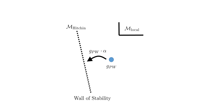
Figure 3: Depiction of the moduli space of solutions to the PW system in a local patch. Each solution is captured by a $G_{\mathbb{C}}$ valued function $g_{PW}(x)$, which determines a complexified flat connection $\mathcal{A}_{PW}=g_{PW}^{-1}dg_{PW}$. Complexified gauge transformations correspond to right multiplication by $G_{\mathbb{C}}$ valued functions $\alpha(x)$ subject to suitable stability conditions. The walls of stability are captured by a local Hitchin system defined on a 2D subspace inside the three-manifold. Perturbations away from this solution define the gauge equivalence classes of solutions in the PW system.

Now, on $\Sigma$, the background $\mathcal{A}_{\text{non-chiral}}$ determines a solution to the Hitchin system (it is a complexified flat connection), and we can first ask whether we can find a localized zero mode here. In fact, this is precisely what was already worked out in reference [46] in the related case of intersecting seven-branes wrapped on Kähler surfaces. The present case is a mild adaptation of that, so we just summarize the main idea. First, we introduce an adjoint-valued $(1,0)$ form Higgs field $\Phi_{z}$. Then, localized matter on the Hitchin curve is obtained from the quotient:

$$\text{5D Zero Mode on }\Sigma\simeq\frac{\mathcal{O}_{\Sigma}^{\text{hol}}\otimes\mathfrak{g}_{\mathbb{C}}}{\left\langle\ker\text{ad}_{\Phi_{z}}\right\rangle},$$ (5.15)

where here, $\mathcal{O}_{\Sigma}^{\text{hol}}\simeq\mathbb{C}[[z]]$ is a formal power series in the local holomorphic coordinate. In the full system on a three-manfold, we will need to work in terms of the power series $\mathbb{C}[[z,\overline{z}]]\simeq\mathbb{C}[[x,y]]$ since $\Phi_{z}$ will typically not depend on just $z=x+iy$. When we do this, we are taking an annihilator condition such as:

$$h+z\chi=0,$$ (5.16)

for $h$ our zero mode and $\chi$ our gauge redundancy parameter. In some non-abelian configurations, it is convenient to instead work with real coordinates $x$ and $y$. Owing to the holomorphic structure of our system, we can equivalently treat such conditions as split up into two separate conditions since we can always restrict $h$ to be real, and separately impose an annihilator constraint from $x$ and $y$.

Perturbing this 5D zero mode, we then reach a 4D chiral mode. From the argument just presented, we can take a family of embeddings of our Riemann surface in the $t$ direction, and by a choice of unitary gauge transformation, we can, without loss of generality, set $A_{t}=0$ so that the complexified connection in this direction is just the Higgs field component $\Phi_{t}$. This also means that the study of localized zero modes reduces to determining the adjoint action by just $\Phi_{t}$. Since the ring of perturbations is now in $\mathcal{O}\otimes\mathfrak{g}_{\mathbb{C}}\simeq\mathbb{C}[[x,y,t]]\otimes\mathfrak{g}_{\mathbb{C}}\simeq\mathbb{C}[[z,\overline{z},t]]\otimes\mathfrak{g}_{\mathbb{C}}$, we reach our proposal for 4D localized zero modes:

$$\text{4D Local Zero Modes}\simeq\frac{\mathcal{O}\otimes\mathfrak{g}_{\mathbb{C}}}{\left\langle\ker\text{ad}_{\Phi_{z}},\ker\text{ad}_{\Phi_{t}}\right\rangle},$$ (5.17)

that is, we quotient by the adjoint action of both $\Phi_{t}$ and $\Phi_{z}$. Observe, however, that we are not quotienting by $\Phi_{\overline{z}}$. Indeed, this is not what we do to extract the 5D zero modes anyway.

Our proposal can now be summarized as follows. We observe that solutions to the Hitchin system on a local 2D subspace serve as walls of stability, and perturbations away from these solutions produce the generic structure of solutions to our backgrounds. Indeed, we have presented a general argument that if we attempt to perform a formal gauge transformation which moves through such a wall, the spectrum of chiral zero modes will reverse signs. This can happen in a local patch, but clearly delineates the “boundary behavior” in the moduli space of the PW system (see figure 3).

In practice, this also means we will need to find a suitable coordinate system such that a Hitchin system can be defined on the subspace in the first place. We expect that this is generically possible because we can also view this procedure of taking complexified gauge transformations as alternatively varying the background metric on the three-manifold until we produce a (singular) limit where the metric collapses to that on a patch of a Riemann surface. In what follows we shall operate under the assumption that all walls of stability in the PW system are captured by a Hitchin system and then extract the localized zero mode spectrum by perturbing away from these walls.

Now, a pleasant feature of the Hitchin system is that there is a spectral equation in terms of a holomorphic section of a bundle $\varphi_{\text{hol}}$. For example, in the case $G=SU(N)$, the spectral equation in the fundamental representation has the form:

$$\det(u_{z}\mathbb{I}_{N}-\varphi_{\text{hol}})=0$$ (5.18)

which is a hypersurface in $T^{\ast}\Sigma$ with $\Sigma$ our “local Hitchin system curve.” Since this is a single holomorphic equation, we can use spectral equation methods to often extract the zero mode content in such cases. Of course, it is also well known that this method can also fail in some T-brane configurations when $\varphi_{\text{hol}}$ is nilpotent [46].

Our plan in the remainder of this section will be to revisit the examples of zero modes treated in section 4. It will hopefully become apparent that the algebraic approach presented here provides a computationally powerful way to characterize zero mode localization in general fluxed backgrounds.

5.3 Examples Revisited

In section 4 we showed how to read off the explicit wave function profile for zero mode solutions in a given background. In this section we use algebraic methods to at least argue for the existence and location of zero modes. We proceed by considering each of the previously studied examples. For ease of exposition, we shall also often set unimportant factors to unity.

5.3.1 Abelian Example

We now analyze the zero mode content of the background obtained in section 3.3.1 with Higgs field:

$$\Phi_{z}\sim\left[\begin{array}[c]{cc}\overline{z}&\\ &-\overline{z}\end{array}\right]\,,\text{ \ \ }\Phi_{t}\sim\left[\begin{array}[c]{cc}-4t&\\ &4t\end{array}\right].$$ (5.19)

To analyze the zero mode content, we first take a complexified gauge transformation to make the background “as close as possible” to that of a Hitchin system on a (non-compact) curve. The first subtlety we face is that the Hessian for $f=z\overline{z}-2t^{2}=x^{2}+y^{2}-2t^{2}$ has signature $(+,+,-)$ in the $(x,y,t)$ coordinates.

Since we are interested in a stable solution to the Hitchin system equations, we need to pick local coordinates which retain a single $+$ and a single $-$ in the Hessian. Consequently, the coordinates for the local Hitchin system must involve the $t$ coordinate (since this is the only $-$ eigenvalue in the Hessian), so we introduce shifted variables: $z^{\prime}=x+it$, $\overline{z}^{\prime}=x-it$, $t^{\prime}=y$, with the 2D subspace for our Hitchin system on $z^{\prime}$ and $\overline{z}^{\prime}$. Observe, however, that since we are discussing an abelian example, these distinctions do not really matter and we can just analyze the annihilator conditions for $\Phi_{x}$, $\Phi_{y}$ and $\Phi_{t}$. We caution that this step is in general not valid and only holds for abelian examples with no flux.

We next determine the structure of the local ring of zero modes in this case. Without loss of generality, we take a zero mode $h$ of charge $q=2$. Along the $z^{\prime}$ direction, the gauge condition is:

$$h+q(1-4)z^{\prime}\chi=0,$$ (5.20)

so we can gauge away any non-trivial $z^{\prime}$ dependence. This means our 5D zero mode is localized along $\mathbb{C}[[z^{\prime}]]/\left\langle z^{\prime}\right\rangle\simeq\mathbb{C}$. Next, we turn to the $t^{\prime}$ annihilator condition:

$$h+qt^{\prime}\eta=0,$$ (5.21)

for $\eta$ a gauge parameter. So, we conclude that the zero modes are captured by the ring:

$$\text{4D Local Zero Mode Space: \ \ }\frac{\mathbb{C}[[z^{\prime},\overline{z}^{\prime},t^{\prime}]]}{\left\langle z^{\prime},\overline{z}^{\prime},t^{\prime}\right\rangle}\simeq\mathbb{C},$$ (5.22)

i.e. a single 4D chiral multiplet localized at the origin $x=y=t=0$. Note that we can also use our perspective on Hitchin systems as destabilizing walls to tell us whether we produced a chiral or anti-chiral zero mode, i.e. based on the sign of a perturbation away from the local system captured by the coordinates $(z^{\prime},\overline{z}^{\prime})$.

5.3.2 Second Abelian Example

As another example using a similar breaking pattern, we next consider the zero modes in the background introduced in section 3.3.2. In this example we took:

$$\Phi_{z}\sim\left[\begin{array}[c]{cc}z&\\ &-z\end{array}\right]\,,\text{ \ \ }\Phi_{t}\sim\left[\begin{array}[c]{cc}0&\\ &0\end{array}\right].$$ (5.23)

Since there is no $t$-dependence in the background fields, we can at best expect a localized mode in codimension six in the local $G_{2}$ background.

The spectral equation for $\Phi_{z}$ in the fundamental representation is:

$$u_{z}^{2}-z^{2}=0.$$ (5.24)

Based on the form of this equation, we expect there to be a localized 5D hypermultiplet at the common zero for the eigenvalues: $z=0$.

We next determine the structure of the local ring of zero modes in this case. Without loss of generality, we take $q=\pm 2$ for our zero mode obtained from adjoint breaking. A priori, the three components of the one-form are each elements in the power series $\mathbb{C}[\left[x,y,t\right]]$ where we also use $z=x+iy$. Given $h$ a charge $q$ zero-form in $\mathcal{O}\simeq\mathbb{C}[\left[x,y,t\right]]$, and $\chi$ a gauge parameter, the algebraic annihilator condition is:

$$h+qz\chi=0,$$ (5.25)

so we conclude that the zero modes are captured by the ring:

$$\text{5D Local Zero Mode Space: \ }\frac{\mathbb{C}[z]}{\left\langle z\right\rangle}\simeq\mathbb{C},$$ (5.26)

i.e. a single 5D hypermultiplet localized at the origin $x=y=0$.

Next consider perturbations to our background $\Phi$ in the $t$ direction:

$$\Phi_{\text{new}}=\Phi+\Phi_{\text{pert}}.$$ (5.27)

We assume that $\Phi_{\text{pert}}$ takes values in the same Cartan subalgebra as $\Phi$. It is immediate that if the perturbations in the $z$ direction are sufficiently small, the only change is in the $t$-dependence of a candidate zero mode profile. This in turn means that for the most generic case where $\Phi_{\text{pert}}$ contains a term proportional to $tdt$, that the 4D local zero mode space is:

$$\text{4D Local Zero Mode Space: \ \ }\frac{\mathbb{C}[[x,y,t]]}{\left\langle x,y,t\right\rangle}\simeq\mathbb{C},$$ (5.28)

as expected.

5.3.3 Fibering a Hitchin Solution

We now generalize the considerations of the above example to consider 5D hypermultiplets which are localized on the $\Sigma$ factor of $M=\Sigma\times I$. We start with a solution to the Hitchin system on $\Sigma$ given by $\Phi_{\text{H}}$ and perturb it to generate a solution to the fluxed PW equations:

$$\Phi_{\text{new}}=\Phi_{\text{H}}+\Phi_{\text{pert}}.$$ (5.29)

Provided $\Phi_{\text{pert}}$ is small, we can first analyze the zero mode content on $\Sigma$, and then extend it to $M$. The annihilator conditions on $\Sigma$ are basically the same as those used in reference [46], so we conclude that the algebraic analysis also correctly captures the zero mode content in this more general situation (almost by design).

5.3.4 T-Brane Example

As our final example, we turn to the fully non-abelian configuration of section 3.3.4 and use our algebraic methods to analyze the zero mode content in this case as well. We first need to introduce a convenient splitting of the PW Higgs field into one associated with a Hitchin system, and then a perturbation away from this choice:

$$\Phi_{\text{PW}}=\Phi_{\text{H}}+\Phi_{\text{pert}}\text{,}$$ (5.30)

where

$$\Phi_{\text{H}}\text{,}\sim\left[\begin{array}[c]{ccc}&\varepsilon dz&\\ zdz&&\\ &&0\end{array}\right]\,,\text{ \ \ }\Phi_{\text{pert}}\sim\left[\begin{array}[c]{ccc}xdx+tdt&&\\ &xdx+tdt&\\ &&-2(xdx+tdt)\end{array}\right].$$ (5.31)

As a one-form, the perturbation points in the $d(x+t)$ direction.

We focus our attention on zero modes in the doublet representation under the breaking pattern $\mathfrak{su}(3)\supset\mathfrak{su}(2)\times\mathfrak{u}(1)$, captured by the entries:

$$\psi=\left[\begin{array}[c]{ccc}\mathcal{\ast}&\mathcal{\ast}&\psi^{+}\\ \mathcal{\ast}&\mathcal{\ast}&\psi^{-}\\ \ast&\ast&\ast\end{array}\right]\,.$$ (5.32)

Denoting by $h$ the corresponding doublet of localized fluctuations and $\chi$ the doublet of gauge parameters entering the annihilator equations, the zero modes fill out entries in $\mathcal{O}\otimes\mathbb{C}^{2}$. In what follows, we treat separately the cases $\varepsilon\neq 0$ and $\varepsilon=0$.

Assuming $\varepsilon\neq 0$, the annihilator conditions coming from $\Phi_{\text{H}}$ are:

$$\Phi_{\text{H}}:\left[\begin{array}[c]{c}h^{+}+\varepsilon\chi^{-}\\ h^{-}+z\chi^{+}\end{array}\right]=0.$$ (5.33)

We are then free to use our gauge parameter $\chi^{-}$ to eliminate $h^{+}$. The second equation tells us:

$$h^{-}+z\chi^{+}=0.$$ (5.34)

so we get only a single zero mode trapped at the origin:

$$\text{5D Local Zero Mode Space: \ \ }\frac{\mathbb{C}[[z]]}{\left\langle z\right\rangle}\simeq\mathbb{C}.$$ (5.35)

Consider next the annihilator conditions coming from $\Phi_{\text{pert}}$. As a one-form, this points in the $d(x+t)$ direction, but since we have already set fluctuations in the $x=0$ direction to zero, it is enough to analyze the annihilator condition in just the $dt$ direction. Additionally, since we have already gauge away $h^{+}$, we are left to analyze just $h^{-}$. We have:

$$\Phi_{\text{pert}}:h^{-}+t\eta^{-}=0,$$ (5.36)

from which it follows that we have a single localized zero mode at the origin:

$$\text{4D Local Zero Mode Space }(\varepsilon\neq 0)\text{: \ \ }\frac{\mathbb{C}[[x,y,t]]}{\left\langle x,y,t\right\rangle}\simeq\mathbb{C}.$$ (5.37)

We now turn to the case of $\varepsilon=0$. The analysis of the $h^{-}$ zero mode is basically the same as the case with $\varepsilon\neq 0$, so we have at least a 4D local zero mode at $x=y=t=0$. Note, however, that now we cannot gauge away $h^{+}$ since our gauge parameter $\chi^{-}$ no longer appears in equation (5.33). So in this case, the algebraic approach can at best point towards partial localization of a zero mode. The full analysis of the system given earlier in section 4 reveals that there is still just a single 4D chiral multiplet localized at the origin, regardless of whether $\varepsilon$ is zero or non-zero.

6 Conclusions

Compactifications of string / M- / F-theory on manifolds of special holonomy produce a wide variety of novel physical systems. In this paper we have used methods from three- and two-dimensional gauge theory to study a broad class of examples in which some important features of the background are captured by non-abelian data, namely T-brane configurations. We have shown that T-brane configurations in $G_{2}$ backgrounds are rather ubiquitous. Additionally, we have seen that the local gauge theory description of $G_{2}$ backgrounds can be understood as a deformation of Calabi–Yau threefolds fibered over an interval. In gauge theory terms this is captured by a gradient flow equation in a deformation of a Hitchin-like system on a Riemann surface. We have also shown how to algebraically extract the zero mode content from these solutions. In the remainder of this section we discuss some avenues of further investigation.

We have presented some evidence that the localized zero mode content can be obtained from local algebraic conditions. It would of course be desirable to have a more systematic derivation of this claim. A related comment is that our analysis provides a potential way to characterize the spectrum of bound states of A-branes in a local Calabi–Yau threefold. It would be very interesting to develop this treatment further.

The general structure of fluxed non-abelian solutions involves fibering a 2D gauge theory over an interval to produce a 3D gauge theory with moduli space matching onto that of a $G_{2}$ background. It is quite natural to extend this procedure to consider 3D PW gauge theories fibered over an interval, thereby producing solutions to 4D gauge theories, which likely build up local $Spin(7)$ backgrounds given by a four-manifold of ADE singularities. In fact, the relevant partially twisted gauge theories have recently been studied in reference [2] (see also [84]).

Along these lines, there are a number of potential physical applications of the results obtained so far. For one, we note that $G_{2}$ backgrounds lead to 4D $\mathcal{N}=1$ vacua of M-theory and 3D $\mathcal{N}=2$ vacua of type II strings. The physical interpretation of the 2D fibration structure also lends itself to a description in terms of interpolating domain wall solutions in one higher dimension. It would be very interesting to further study the properties of these domain walls.

One of the main results of this work is that it is possible to generate localized matter using T-brane configurations of the fluxed PW system. This in turn suggests a new method for building global M-theory backgrounds with localized matter in which some of the well-known issues with constructing codimension seven singularities are simply bypassed. That being said, there do appear to be deformations which could convert a geometric codimension six singularity back into a codimension seven singularity. We refer to [9] for a discussion on how such a solution could be engineered from appropriate paths in the moduli space of the local gauge theory.

In this work we have given an algebraic characterization of zero modes in local $G_{2}$ backgrounds. That being said, there are a few outstanding items which would clearly be interesting to develop further. One concerns the full matter spectrum, even in the case of a compact three-manifold of ADE singularities in a local $G_{2}$ background. In physical terms, the matter spectrum is constrained by anomaly cancellation considerations, but at the moment we have treated each background as a freely adjustable feature of our models. Presumably this is encoded in the geometry of the spectral equations for the Higgs field, but it would be interesting to explicitly verify that this is the case.

Indeed, in the context of intersecting seven-branes in F-theory, spectral cover methods have been fruitfully applied in developing a streamlined analysis of many features of localized matter. Since M-theory on a $G_{2}$ background and F-theory on an elliptically fibered Calabi–Yau fourfold both give rise to 4D $\mathcal{N}=1$ vacua, it is natural to expect an explicit map which converts the local geometric methods of one description into the other. The common link in this thread is the appearance of a corresponding “local” heterotic dual. Developing the precise form of this match would likely shed light on local methods in M-theory, F-theory, and heterotic vacua.

It is natural to expect the considerations here to match on to some macroscopic features as captured by supergravity solutions. Indeed, there is a class of supergravity solutions known as “M3-branes” with a real codimension four singularity [38, 39]. It would be very interesting to study how these explicit supergravity solutions match on to features appearing in the PW system.

Finally, we have exclusively focused on the local geometry of $G_{2}$ backgrounds. We have also seen that at least from the perspective of the gauge theory, there is no reason to restrict attention to $M$ a rational homology sphere. This suggests a possible generalization of the TCS construction, as motivated by physical considerations. It is tempting to ask whether a set of consistency relations can be stated which would allow one to piece together these local geometries to form a more global characterization of $G_{2}$ backgrounds with chiral matter.

References

- [1] P. Candelas, G. T. Horowitz, A. Strominger, and E. Witten, “Vacuum Configurations for Superstrings,” Nucl. Phys. B258 (1985) 46–74.
- [2] J. J. Heckman, C. Lawrie, L. Lin, and G. Zoccarato, “F-theory and Dark Energy,” arXiv:1811.01959 [hep-th].
- [3] J. J. Heckman, C. Lawrie, L. Lin, J. Sakstein, and G. Zoccarato, “Pixelated Dark Energy,” arXiv:1901.10489 [hep-th].
- [4] F. Bonetti, T. W. Grimm, and T. G. Pugh, “Non-Supersymmetric F-Theory Compactifications on Spin(7) Manifolds,” JHEP 01 (2014) 112, arXiv:1307.5858 [hep-th].
- [5] F. Bonetti, T. W. Grimm, E. Palti, and T. G. Pugh, “F-Theory on Spin(7) Manifolds: Weak-Coupling Limit,” JHEP 02 (2014) 076, arXiv:1309.2287 [hep-th].
- [6] P. Berglund, T. Hubsch, and D. Minic, “On Stringy de Sitter Spacetimes,” arXiv:1902.08617 [hep-th].
- [7] P. Berglund, T. Hubsch, and D. Minic, “Dark Energy and String Theory,” arXiv:1905.08269 [hep-th].
- [8] C. Vafa, “Evidence for F theory,” Nucl. Phys. B469 (1996) 403–418, arXiv:hep-th/9602022.
- [9] R. Barbosa, “A Deformation Family for Closed -Structures on ADE Fibrations,” arXiv:1910.10742 [math.DG].
- [10] R. Barbosa, Deformations of -Structures, String Dualities and Flat Higgs Bundles. PhD thesis, University of Pennsylvania, 2019.
- [11] D.-E. Diaconescu, R. Donagi, R. Dijkgraaf, C. Hofman, and T. Pantev, “Geometric transitions and integrable systems,” Nucl. Phys. B752 (2006) 329–390, arXiv:hep-th/0506196.
- [12] D.-E. Diaconescu, R. Donagi, and T. Pantev, “Intermediate Jacobians and ADE Hitchin Systems,” arXiv:hep-th/0607159.
- [13] L. Foscolo, M. Haskins, and J. Nordström, “Complete non-compact G2-manifolds from asymptotically conical Calabi-Yau 3-folds,” arXiv:1709.04904 [math.DG].
- [14] L. Foscolo, M. Haskins, and J. Nordström, “Infinitely many new families of complete cohomogeneity one -manifolds: analogues of the Taub-NUT and Eguchi-Hanson spaces,” arXiv:1805.02612 [math.DG].
- [15] A. Brandhuber, J. Gomis, S. S. Gubser, and S. Gukov, “Gauge theory at large N and new G(2) holonomy metrics,” Nucl. Phys. B611 (2001) 179–204, arXiv:hep-th/0106034.
- [16] M. Cvetič, G. W. Gibbons, H. Lu, and C. N. Pope, “A Unification of the Deformed and Resolved Conifolds,” Phys. Lett. B534 (2002) 172–180, arXiv:hep-th/0112138.
- [17] M. Cvetic, G. W. Gibbons, H. Lu, and C. N. Pope, “New Complete Noncompact Spin(7) Manifolds,” Nucl. Phys. B620 (2002) 29–54, arXiv:hep-th/0103155.
- [18] M. Cvetic, G. W. Gibbons, H. Lu, and C. N. Pope, “New Cohomogeneity One Metrics with Spin(7) Holonomy,” J. Geom. Phys. 49 (2004) 350–365, arXiv:math/0105119 [math-dg].
- [19] M. Cvetic, G. W. Gibbons, H. Lu, and C. N. Pope, “Special Holonomy Spaces and M Theory,” in Unity from duality: Gravity, gauge theory and strings. Proceedings, NATO Advanced Study Institute, Euro Summer School, 76th session, Les Houches, France, July 30-August 31, 2001, pp. 523–545. 2002. arXiv:hep-th/0206154.
- [20] M. Cvetič, G. Shiu, and A. M. Uranga, “Three Family Supersymmetric Standard - Like Models from Intersecting Brane Worlds,” Phys. Rev. Lett. 87 (2001) 201801, arXiv:hep-th/0107143.
- [21] M. Cvetic, G. Shiu, and A. M. Uranga, “Chiral Four-Dimensional Supersymmetric Type IIA Orientifolds from Intersecting D6-Branes,” Nucl. Phys. B615 (2001) 3–32, arXiv:hep-th/0107166.
- [22] M. Cvetič, G. Shiu, and A. M. Uranga, “Chiral Type II Orientifold Constructions as M Theory on Holonomy Spaces,” in Supersymmetry and unification of fundamental interactions. Proceedings, 9th International Conference, SUSY’01, Dubna, Russia, June 11-17, 2001, pp. 317–326. 2001. arXiv:hep-th/0111179.
- [23] T. Pantev and M. Wijnholt, “Hitchin’s Equations and M-Theory Phenomenology,” J. Geom. Phys. 61 (2011) 1223–1247, arXiv:0905.1968 [hep-th].
- [24] A. P. Braun, S. Cizel, M. Hubner, and S. Schäfer-Nameki, “Higgs Bundles for M-theory on -Manifolds,” arXiv:1812.06072 [hep-th].
- [25] A. Kovalev, “Twisted connected sums and special Riemannian holonomy,” J. Reine Angew. Math. 565 (2003) 125–160.
- [26] A. Corti, M. Haskins, J. Nordström, and T. Pacini, “Asymptotically cylindrical Calabi-Yau 3-folds from weak Fano 3-folds,” Geom. Topol. 17 no. 4, (2013) 1955–2059.
- [27] A. Corti, M. Haskins, J. Nordström, and T. Pacini, “-manifolds and associative submanifolds via semi-Fano 3-folds,” Duke Math. J. 164 no. 10, (2015) 1971–2092.
- [28] J. Halverson and D. R. Morrison, “The landscape of M-theory compactifications on seven-manifolds with G2 holonomy,” JHEP 04 (2015) 047, arXiv:1412.4123 [hep-th].
- [29] J. Halverson and D. R. Morrison, “On gauge enhancement and singular limits in G2 compactifications of M-theory,” JHEP 04 (2016) 100, arXiv:1507.05965 [hep-th].
- [30] A. P. Braun, “Tops as building blocks for G2 manifolds,” JHEP 10 (2017) 083, arXiv:1602.03521 [hep-th].
- [31] T. C. da C. Guio, H. Jockers, A. Klemm, and H.-Y. Yeh, “Effective Action from M-Theory on Twisted Connected Sum G2-Manifolds,” Commun. Math. Phys. 359 no. 2, (2018) 535–601, arXiv:1702.05435 [hep-th].
- [32] A. P. Braun and M. Del Zotto, “Mirror Symmetry for -Manifolds: Twisted Connected Sums and Dual Tops,” JHEP 05 (2017) 080, arXiv:1701.05202 [hep-th].
- [33] A. P. Braun and S. Schäfer-Nameki, “Compact, Singular -Holonomy Manifolds and M/Heterotic/F-Theory Duality,” JHEP 04 (2018) 126, arXiv:1708.07215 [hep-th].
- [34] A. P. Braun and M. Del Zotto, “Towards Generalized Mirror Symmetry for Twisted Connected Sum Manifolds,” JHEP 03 (2018) 082, arXiv:1712.06571 [hep-th].
- [35] A. P. Braun, M. Del Zotto, J. Halverson, M. Larfors, D. R. Morrison, and S. Schäfer-Nameki, “Infinitely many M2-instanton corrections to M-theory on G2-manifolds,” JHEP 09 (2018) 077, arXiv:1803.02343 [hep-th].
- [36] M.-A. Fiset, “Superconformal algebras for twisted connected sums and G2 mirror symmetry,” JHEP 12 (2018) 011, arXiv:1809.06376 [hep-th].
- [37] B. S. Acharya, A. P. Braun, E. E. Svanes, and R. Valandro, “Counting Associatives in Compact Orbifolds,” arXiv:1812.04008 [hep-th].
- [38] M. Cvetič, G. W. Gibbons, H. Lu, and C. N. Pope, “Supersymmetric M3-branes and Manifolds,” Nucl. Phys. B620 (2002) 3–28, arXiv:hep-th/0106026.
- [39] M. Cvetič, G. W. Gibbons, H. Lu, and C. N. Pope, “Cohomogeneity One Manifolds of Spin(7) and Holonomy,” Phys. Rev. D65 (2002) 106004, arXiv:hep-th/0108245.
- [40] Z. W. Chong, M. Cvetič, G. W. Gibbons, H. Lu, C. N. Pope, and P. Wagner, “General Metrics of Holonomy and Contraction limits,” Nucl. Phys. B638 (2002) 459–482, arXiv:hep-th/0204064.
- [41] B. S. Acharya, “M Theory, Joyce Orbifolds and Super Yang-Mills,” Adv. Theor. Math. Phys. 3 (1999) 227–248, arXiv:hep-th/9812205.
- [42] B. S. Acharya and E. Witten, “Chiral fermions from manifolds of G(2) holonomy,” arXiv:hep-th/0109152 [hep-th].
- [43] P. S. Aspinwall and R. Y. Donagi, “The Heterotic string, the tangent bundle, and derived categories,” Adv. Theor. Math. Phys. 2 (1998) 1041–1074, arXiv:hep-th/9806094.
- [44] R. Donagi, S. Katz, and E. Sharpe, “Spectra of D-branes with higgs vevs,” Adv. Theor. Math. Phys. 8 no. 5, (2004) 813–859, arXiv:hep-th/0309270 [hep-th].
- [45] S. Cecotti, M. C. N. Cheng, J. J. Heckman, and C. Vafa, “Yukawa Couplings in F-theory and Non-Commutative Geometry,” arXiv:0910.0477 [hep-th].
- [46] S. Cecotti, C. Cordova, J. J. Heckman, and C. Vafa, “T-Branes and Monodromy,” JHEP 07 (2011) 030, arXiv:1010.5780 [hep-th].
- [47] R. Donagi and M. Wijnholt, “Gluing Branes, I,” JHEP 05 (2013) 068, arXiv:1104.2610 [hep-th].
- [48] L. B. Anderson, J. J. Heckman, and S. Katz, “T-Branes and Geometry,” JHEP 05 (2014) 080, arXiv:1310.1931 [hep-th].
- [49] A. Collinucci and R. Savelli, “T-branes as branes within branes,” JHEP 09 (2015) 161, arXiv:1410.4178 [hep-th].
- [50] M. Cicoli, F. Quevedo, and R. Valandro, “De Sitter from T-branes,” JHEP 03 (2016) 141, arXiv:1512.04558 [hep-th].
- [51] J. J. Heckman, T. Rudelius, and A. Tomasiello, “6D RG Flows and Nilpotent Hierarchies,” JHEP 07 (2016) 082, arXiv:1601.04078 [hep-th].
- [52] A. Collinucci, S. Giacomelli, R. Savelli, and R. Valandro, “T-branes through 3d mirror symmetry,” JHEP 07 (2016) 093, arXiv:1603.00062 [hep-th].
- [53] I. Bena, J. Blaback, R. Minasian, and R. Savelli, “There and back again: A T-brane’s tale,” JHEP 11 (2016) 179, arXiv:1608.01221 [hep-th].
- [54] F. Marchesano and S. Schwieger, “T-branes and -corrections,” JHEP 11 (2016) 123, arXiv:1609.02799 [hep-th].
- [55] L. B. Anderson, J. J. Heckman, S. Katz, and L. Schaposnik, “T-Branes at the Limits of Geometry,” JHEP 10 (2017) 058, arXiv:1702.06137 [hep-th].
- [56] A. Collinucci, S. Giacomelli, and R. Valandro, “T-branes, monopoles and S-duality,” JHEP 10 (2017) 113, arXiv:1703.09238 [hep-th].
- [57] M. Cicoli, I. Garcìa-Etxebarria, C. Mayrhofer, F. Quevedo, P. Shukla, and R. Valandro, “Global Orientifolded Quivers with Inflation,” JHEP 11 (2017) 134, arXiv:1706.06128 [hep-th].
- [58] F. Marchesano, R. Savelli, and S. Schwieger, “Compact T-branes,” JHEP 09 (2017) 132, arXiv:1707.03797 [hep-th].
- [59] M. Cvetic, J. J. Heckman, and L. Lin, “Towards Exotic Matter and Discrete Non-Abelian Symmetries in F-theory,” JHEP 11 (2018) 001, arXiv:1806.10594 [hep-th].
- [60] J. J. Heckman, T. Rudelius, and A. Tomasiello, “Fission, Fusion, and 6D RG Flows,” JHEP 02 (2019) 167, arXiv:1807.10274 [hep-th].
- [61] F. Apruzzi, F. Hassler, J. J. Heckman, and T. B. Rochais, “Nilpotent Networks and 4D RG Flows,” arXiv:1808.10439 [hep-th].
- [62] F. Carta, S. Giacomelli, and R. Savelli, “SUSY enhancement from T-branes,” JHEP 12 (2018) 127, arXiv:1809.04906 [hep-th].
- [63] F. Marchesano, R. Savelli, and S. Schwieger, “T-branes and defects,” arXiv:1902.04108 [hep-th].
- [64] R. Donagi and E. Witten, “Supersymmetric Yang-Mills theory and integrable systems,” Nucl. Phys. B460 (1996) 299–334, arXiv:hep-th/9510101.
- [65] R. C. Mclean, “Deformations of calibrated submanifolds,” Commun. Analy. Geom 6 (1996) 705–747.
- [66] J. J. Heckman, “Lectures on Geometric Engineering,” in Graduate Summer School on the Mathematics and Physics of Hitchin Systems at the Simons Center for Geometry and Physics. 2019. http://scgp.stonybrook.edu/archives/25133.
- [67] M. Blau and G. Thompson, “Aspects of Topological Gauge Theories and D-Branes,” Nucl. Phys. B492 (1997) 545–590, arXiv:hep-th/9612143.
- [68] M. Bershadsky, C. Vafa, and V. Sadov, “D-branes and topological field theories,” Nucl. Phys. B463 (1996) 420–434, arXiv:hep-th/9511222.
- [69] D. Gaiotto and E. Witten, “Knot Invariants from Four-Dimensional Gauge Theory,” Adv. Theor. Math. Phys. 16 no. 3, (2012) 935–1086, arXiv:1106.4789 [hep-th].
- [70] S. K. Donaldson, “Twisted harmonic maps and the self-duality equations,” Proc. London Math. Soc. (3) 55 no. 1, (1987) 127–131.
- [71] K. Corlette, “Flat -bundles with canonical metrics,” Journal of Differential Geometry 28 no. 3, (1988) 361–382.
- [72] S. K. Donaldson, “Anti self-dual Yang-Mills connections over complex algebraic surfaces and stable vector bundles,” Proc. London Math. Soc. (3) 50 no. 1, (1985) 1–26.
- [73] K. Uhlenbeck and S.-T. Yau, “On the existence of Hermitian-Yang-Mills connections in stable vector bundles,” Comm. Pure Appl. Math. 39 no. S, suppl., (1986) S257–S293. Frontiers of the mathematical sciences: 1985 (New York, 1985).
- [74] N. J. Hitchin, “The Selfduality equations on a Riemann surface,” Proc. Lond. Math. Soc. 55 (1987) 59–131.
- [75] C. T. Simpson, “Higgs bundles and local systems,” Inst. Hautes Études Sci. Publ. Math. no. 75, (1992) 5–95.
- [76] I. Smith, R. P. Thomas, and S.-T. Yau, “Symplectic conifold transitions,” Journal of Differential Geometry 62 no. 2, (2002) 209–242.
- [77] S. Andriolo, G. Shiu, H. Triendl, T. Van Riet, G. Venken, and G. Zoccarato, “Compact G2 holonomy spaces from SU(3) structures,” JHEP 03 (2019) 059, arXiv:1811.00063 [hep-th].
- [78] M. Grana, “Flux compactifications in string theory: A Comprehensive review,” Phys. Rept. 423 (2006) 91–158, arXiv:hep-th/0509003.
- [79] M. F. Atiyah, V. K. Patodi, and I. M. Singer, “Spectral asymmetry and Riemannian Geometry 1,” Math. Proc. Cambridge Phil. Soc. 77 (1975) 43.
- [80] H. Hayashi, T. Kawano, R. Tatar, and T. Watari, “Codimension-3 Singularities and Yukawa Couplings in F-theory,” Nucl. Phys. B823 (2009) 47–115, arXiv:0901.4941 [hep-th].
- [81] R. Donagi and M. Wijnholt, “Higgs Bundles and UV Completion in F-Theory,” Commun. Math. Phys. 326 (2014) 287–327, arXiv:0904.1218 [hep-th].
- [82] J. Marsano, N. Saulina, and S. Schafer-Nameki, “Monodromies, Fluxes, and Compact Three-Generation F-theory GUTs,” JHEP 08 (2009) 046, arXiv:0906.4672 [hep-th].
- [83] R. Blumenhagen, T. W. Grimm, B. Jurke, and T. Weigand, “Global F-theory GUTs,” Nucl. Phys. B829 (2010) 325–369, arXiv:0908.1784 [hep-th].
- [84] S. Gukov and J. Sparks, “M-Theory on Spin(7) Manifolds,” Nucl. Phys. B625 (2002) 3–69, arXiv:hep-th/0109025.