Memories of initial states and density imbalance in dynamics of interacting disordered systems

Abstract

We study the dynamics of one and two dimensional disordered lattice bosons/fermions initialized to a Fock state with a pattern of $1$ and $0$ particles on $A$ and ${\bar{A}}$ sites. For non-interacting systems we establish a universal relation between the long time density imbalance between $A$ and ${\bar{A}}$ site, $I(\infty)$, the localization length $\xi_{l}$, and the geometry of the initial pattern. For alternating initial pattern of $1$ and $0$ particles in 1 dimension, $I(\infty)=\tanh[a/\xi_{l}]$, where $a$ is the lattice spacing. For systems with mobility edge, we find analytic relations between $I(\infty)$, the effective localization length $\tilde{\xi}_{l}$ and the fraction of localized states $f_{l}$. The imbalance as a function of disorder shows non-analytic behaviour when the mobility edge passes through a band edge. For interacting bosonic systems, we show that dissipative processes lead to a decay of the memory of initial conditions. However, the excitations created in the process act as a bath, whose noise correlators retain information of the initial pattern. This sustains a finite imbalance at long times in strongly disordered interacting systems.

A generic quantum many body system, initialized to a typical state, forgets the memory of the initial state. In the long time limit, local observables in the system can be described by an ensemble of states with a probability measure determined by its Hamiltonian. This basic tenet of equilibrium statistical mechanics has been challenged in recent years in strongly disordered interacting quantum systems, a phenomenon called many body localization(MBL) BaskoAleiner ; Mirlin2005 ; pal_huse ; MBL_review1 ; MBL_review2 ; MBL_review3 .

While theoretical studies of MBL have focussed on the properties of many body eigenstates in the middle of the spectrum MBL_review1 ; MBL_review2 ; MBL_review3 ; pal_huse , it is impossible to experimentally access these states individually. In experiments on MBL in cold atoms MBLexpt1 ; MBLexpt2 ; MBLexpt3 ; MBLexpt4 ; MBLexpt5 ; MBLexpt11 , the system is initialized in a Fock state, which has $1$ particle on a set of lattice sites (say $A$) and $0$ particles on the rest (say $\bar{A}$). As the system evolves, the density imbalance between $A$ and $\bar{A}$ sites, normalized by average density, is measured. The Hamiltonian of the system (averaged over disorder) does not distinguish between $A$ and $\bar{A}$ sites; in a thermal state the imbalance should be $0$. A finite imbalance in the long time limit implies that the system remembers the initial condition and indicates absence of thermalization in the system.

In this paper, we use a new extension of Keldysh field theory  chakraborty2 to understand imbalance dynamics in systems with random or incommensurate potentials. For localized non-interacting systems, we derive a universal relation between the long time density imbalance, the localization length and the geometry of the initial density pattern. For the initial patterns used in 1-d and 2-d experiments, we obtain analytic relations between localization length and long time imbalance. Near a localization-delocalization transition, the imbalance scales as the inverse localization length. We test our theory using the random potential Anderson model AL_original in 1 and 2 dimensions and the Aubry Andre model AA_original in 1 dimension.

In systems with a mobility edge MAA ; Mukerjeereview , only the localized states contribute to long time imbalance. The one particle Green’s functions, projected on these states, decay exponentially with distance. This defines an “effective” localization length. The imbalance, divided by the fraction of localized states in the system, is given by the same analytic relations with this effective localization length. This leads to non-analyticites in the imbalance as a function of disorder strength, when the mobility edge passes through a band edge.

Finally, we consider imbalance dynamics in a Bose Hubbard model with an incommensurate potential. We use a conserving approximation conserving_KadanoffBaym , keeping the lowest order processes leading to dissipative and stochastic dynamics. Naively one would expect the memory of the initial state to decay, as the Green’s functions which propagate this memory decay in time. However, as the quasiparticles decay, they create excitations which act as a bath for the rest of the quasiparticles. The noise fluctuations of this bath remembers the initial conditions at strong disorder, and sustain the finite long time imbalance.

Imbalance dynamics in MBL systems has been treated theoretically using exact diagonalization(ED), DMRG MBLexpt1 ; DasSarmadyn and in Hartree-Fock approximation HartreeFock . However, ED and DMRG does not provide insight about the mechanism that sustains the imbalance in interacting systems, while the Hartree Fock approximation ignores the dissipative and stochastic processes included in this work.

Imbalance and Localization Length: We consider non-interacting particles with

$$H=-J\sum_{\langle ij\rangle}a^{\dagger}_{i}a_{j}+\sum_{i}v(i)a^{\dagger}_{i}a_{i},$$ (1)

where $a^{\dagger}_{i}$ is the particle creation operator on lattice site $i$, $J$ is the nearest neighbour hopping and $v(i)$ is a local potential.

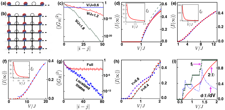
Figure 1: Initial density profiles for imbalance dynamics in (a) linear chain and (b) square lattice. The solid(hollow) dots are particles (vacancies). (c) $\langle|G^{\infty}_{R}(i,j)|^{2}\rangle$ for Aubry Andre model as a function of $|i-j|$. For $V/J=0.6$, it saturates to a finite value; for $V/J=1.2,1.8$ it decays exponentially. (d)-(f): Long time imbalance $\langle I(\infty)\rangle$ as function of $V/J$ obtained from Eq. 3 (solid dots) for (d) Aubry Andre model, (e) 1-d Anderson model and (f) square lattice Anderson model. The solid lines are Eq. 5 (d,e) or Eq. 6 (f) with $\xi_{l}$ obtained from fitting $|G_{R}|^{2}$ (see inset for $\xi_{l}$ vs $V/J$). The dashed line in (d) uses $\xi_{l}/a=log[V/J]$. (g) $\langle|G^{\infty}_{R}|^{2}\rangle$ in the modified Aubry Andre model with mobility edge as a function of distance ($V/J=1.2$ and $\nu=0.4$). The full Greens function (which saturates) and its projection onto the localized states (which decay exponentially) are both shown. (h) $\langle I(\infty)\rangle$ for the modified Aubry Andre model as a function of $V/J$ for $\nu=0.4,0.6$ obtained from (i) Eq. 3 (solid dots) (ii) Eq. 7(solid lines). $\xi_{l}$ is obtained from fits of localized contributions in $|G_{R}|^{2}$. (i) The fraction of localized states ($f_{l}$), the long time imbalance $\langle I\rangle$(multiplied by $2$ to plot on same scale)and the derivative $d\langle I\rangle/dV$ as a function of $V/J$ for the modified Aubry Andre model ($\nu=0.3$). The values of $V/J$, where the mobility edge leaves or enters a band are marked by derivative discontinuities in $f_{l}$ and $\langle I\rangle$. All data are averaged over $100$ disorder configurations. 1-d data are for $1000$ sites and 2-d data is for a $100\times 100$ lattice.

We will study dynamics of this system within the Schwinger Keldysh field theory Kamenevbook , which has two independent one particle correlators: (a) the retarded Green’s function, $G_{R}(i,t;j,t^{\prime})$, which is the amplitude of propagating a particle to site $i$ at time $t$ provided the particle was at site $j$ at time $t^{\prime}$, without creating additional excitations, and (b) the Keldysh Green’s function $G_{K}(i,t;j,t^{\prime})$, which represents the actual amplitude of exchanging a particle between site $i$ at time $t$ and site $j$ at time $t^{\prime}$. $G_{K}(i,t;j,t)$ is related to densities and currents in the system; e.g. for bosons (fermions), the local density $n_{i}(t)=(\pm 1/2)[iG_{K}(i,t;i,t)-1]$.

The system is initialized to a Fock state, where $n_{i}(0)=1/2(1+\sigma_{i})$, with $\sigma_{i}=\pm 1$ if $i\in A(\bar{A})$. We use an extension of Keldysh field theory, which can explicitly keep track of arbitrary initial conditions in quantum dynamics  chakraborty2 . Here, $G_{R}(i,t;j,t^{\prime})=\sum_{n}\phi^{\ast}_{n}(i)\phi_{n}(j)e^{-iE_{n}(t-t^{\prime})}$, where $E_{n}$ and $\phi_{n}(i)$ are the energy levels and corresponding wavefunctions. The Keldysh Green’s function $G_{K}$ carries the information of the initial density matrix and is given by

$$iG_{K}(i,t;j,t^{\prime}) = \sum_{k}G_{R}(i,t;k,0)G_{R}^{\ast}(j,t^{\prime};k,0)[1\pm 2n_{k}(0)],$$

$$n_{i}(t) = \sum_{k}|G_{R}(i,t;k,0)|^{2}n_{k}(0).$$ (2)

Note that the expression for local density is same for bosons and fermions. Hence, all the statements about imbalance dynamics in non-interacting systems are independent of statistics of particles. For a closed system with equal number of $A$ and $\bar{A}$ sites, the density imbalance, averaged over disorder, is

$$\langle I(t)\rangle=\frac{2}{N}\sum_{k\in A,i}\sigma_{i}\langle|G_{R}(i,t;k,0)|^{2}\rangle.$$ (3)

The Green’s functions can be calculated from the knowledge of energy eigenfunction in each disorder configuration, yielding a “numerical” estimate of imbalance. $G_{R}(i,t;k,0)$ is the solution to Anderson’s original problem AL_original : it is the wavefunction at site $i$ and time $t$ of a particle initially localized at $k$. As $t\rightarrow\infty$, in the localized phase, $\langle|G^{\infty}_{R}(i,k)|^{2}\rangle=\langle\sum_{n}|\phi_{n}(i)\phi^{\ast}_{n}(k)|^{2}\rangle\sim e^{-2|r_{i}-r_{k}|/\xi_{l}}$. This decay defines the localization length $\xi_{l}$. The long time imbalance

$$\langle I(\infty)\rangle=\frac{2}{N}\sum_{i}\sum_{k\in A}\sigma_{i}e^{-\frac{2|r_{i}-r_{k}|}{\xi_{l}}}.$$ (4)

This is the universal relation between the long time imbalance, the localization length and the geometry of the initial pattern. We will now consider some specific initial patterns that have been used in the cold atom experiments on MBL MBLexpt1 ; MBLexpt4 .

1-d chain with alternating pattern: We consider a linear chain with an initial state which has alternating $|1,0,1,0,...\rangle$ pattern  MBLexpt1 , as shown in Fig. 1(a). Assuming a large chain where boundary effects can be neglected (see SM for details), the sum in Eq. 4 gives

$$\langle I(\infty)\rangle=\tanh\left(\frac{a}{\xi_{l}}\right).$$ (5)

From this “analytic” estimate, we see that as $\xi_{l}/a\rightarrow\infty$, $\langle I(\infty)\rangle\sim\frac{a}{\xi_{l}}\rightarrow 0$; i.e. (i) the memory retention is related to localization and (ii) close to a localization-delocalization transition, the scaling of the Lyapunov exponent Thouless1983 $\gamma=a/\xi_{l}$ governs the behaviour of the density imbalance.

We first consider the Aubry Andre model AA_original , with an incommensurate $v(i)=V\cos[2\pi\alpha i+\theta]$, where $\alpha=(\sqrt{5}+1)/2$ is the golden mean, and $\theta$ is a uniformly distributed random phase. This model, which is implemented in cold atom experiments MBLexpt1 , has a localization-delocalization transition at $V/J=1$ AA_original . This can be clearly seen in Fig. 1(c), where we plot $\langle|G^{\infty}_{R}(i,j)|^{2}\rangle$ as a function of $|i-j|$. For $V/J=0.6$, where the system is delocalized, $\langle|G^{\infty}_{R}|^{2}\rangle$ saturates to a finite value at large distances, whereas it shows an exponential decay for $V/J>1$. In Fig. 1 (d), we plot the long time imbalance as a function of $V/J$ obtained using the numerical estimate from Eq. 3 (solid dots) . We also plot the analytic answer from Eq. 5 with $\xi_{l}$ obtained from (i) fitting $\langle|G^{\infty}_{R}|^{2}\rangle$ (solid line)[see inset for $\xi_{l}$ vs $V/J$] and (ii) a duality relation  AA_duality $\xi_{l}=a~{}log[V/J]$ (dashed line). The analytic answer matches the numerical estimate for $\xi_{l}/a>1$. We also consider the 1-d Anderson model AL_original where each $v(i)$ is an independent random variable, with $P[v(i)]=\Theta[V^{2}/4-v^{2}(i)]1/V$. This system is localized for any $V/J$, with a localization length $\xi_{l}/a\sim(V/J)^{-2}$ illcondmat for weak disorder (see inset of Fig. 1 (e)). In Fig. 1 (e) we plot the long time imbalance obtained from Eq. 3 (solid dots) and Eq. 5(solid line) and find good quantitative match between these estimates.

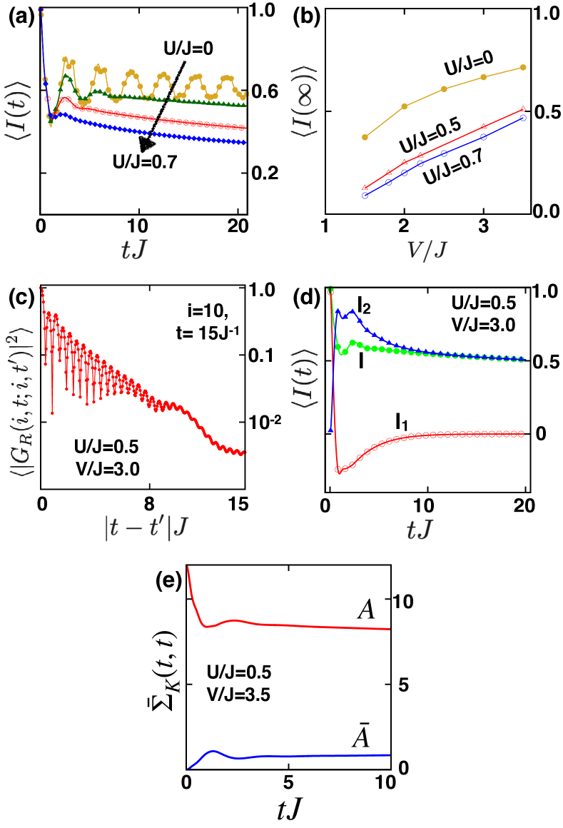
Figure 2: (a) $I(t)$ for Bosons in an Aubry Andre Hubbard model with $V/J=2.5$ and $U/J=0.0,~{}0.3,~{}0.5,~{}0.7$. For finite $U$, the imbalance decays exponentially to a finite value. (b) The long time imbalance $\langle I(\infty)\rangle$ as function of $V/J$ for different values of $U/J$. (c) The exponential decay in time for $G_{R}$ due to dissipative process. (d) The contribution to imbalance due to (i) the direct decay of initial correlations $I_{1}$ and (ii) stochastic fluctuation due to effective bath $I_{2}$. The long time imbalance is dominated by $I_{2}$.(e) The space-time local part of $\Sigma_{K}$, averaged over $A$ and ${\bar{A}}$ sites. The bath clearly distinguishes between $A$ and ${\bar{A}}$ sites at long times. All data in (a)-(d) are for $N=20$ sites and averaged over $50$ configurations. (e) is obtained from $N=10$ site system averaged over $200$ samples.

Disordered Square Lattice: We consider the Anderson model of uniformly distributed random potentials on a square lattice AL_original . This model is localized for all $V/J$, with $\langle|G^{\infty}_{R}(r)|^{2}\rangle\sim e^{-2\sqrt{r_{x}^{2}+r_{y}^{2}}/\xi_{l}}$, and $\xi_{l}\sim a~{}e^{J^{2}/V^{2}}$ illcondmat . We consider the experimentally relevant MBLexpt2 ; MBLexpt4 initial density pattern of alternating chains which have $1$ and $0$ particles on each site, as shown in Fig 1(b). The long time imbalance

$$\langle I(\infty)\rangle=\sum_{n_{x},n_{y}=-\infty}^{\infty}(-1)^{n_{x}}e^{-\frac{2a}{\xi_{l}}\sqrt{n_{x}^{2}+n_{y}^{2}}}.$$ (6)

While this sum cannot be done analytically, numerical evaluation (see SM for details) shows $\langle I(\xi_{l})\rangle\sim(\sqrt{32}/\pi^{2})(a/\xi_{l})$ for $\xi_{l}\gg a$. In Fig 1(f), we plot the imbalance obtained from Eq. 3 (solid dots) together with that obtained from Eq. 6 (solid lines), with $\xi_{l}$ (see inset) obtained from exponential fit of the $\langle|G^{\infty}_{R}|^{2}\rangle$. The two approaches match till $V/J=5$, when $\xi_{l}\sim 100a$ and our $100\times 100$ system is effectively delocalized, The cold atom experiments, which are restricted to similar sizes, may also see effective delocalization at this scale.

Mobility Edges and Imbalance: We now turn our attention to the modified Aubry Andre model MAA ; Mukerjeereview in 1d, where $v(i)=V\cos[2\pi\alpha i+\theta]/(1-\nu\cos[2\pi\alpha i+\theta])$, with $-1<\nu<1$. $\nu=0$ corresponds to the Aubry Andre model discussed before. At low $V/J$ the model has delocalized states, for intermediate values of $V/J$ it supports a mobility edge at $E_{c}=2(J-V)/\nu$ MAA , which is an energy threshold separating localized and delocalized states. At large $V/J$ all states are localized in the system. In Fig. 1 (g), we plot $\langle|G^{\infty}_{R}|^{2}\rangle$ of the system as a function of distance for $V/J=1.2$ and $\nu=0.4$, where there is a mobility edge. The long distance behaviour of $\langle|G^{\infty}_{R}|^{2}\rangle$ is dominated by delocalized states and saturates to a constant. In the same figure, we also plot the contribution to $\langle|G^{\infty}_{R}|^{2}\rangle$ from states above the mobility edge, which clearly shows an exponential decay. This decay can be used to extract an “effective” localization length $\tilde{\xi}_{l}$ for the system. The imbalance in this case is given by

$$\langle I(\infty)\rangle=f_{l}\tanh\left(\frac{a}{\tilde{\xi}_{l}}\right),$$ (7)

where $f_{l}$ is the fraction of localized states. In Fig. 1 (h), we plot $\langle I(\infty)\rangle$ as a function of $V/J$ for $\nu=0.4,0.6$. The solid dots (Eq. 3) and the solid lines (Eq. 7) track each other. The imbalance goes to $0$ when all states are delocalized at low $V/J$. At large $V/J$, the curve approaches the $\nu=0$ answer.

There is a clear non-analytic feature of the imbalance as a function of $V/J$, which coincides with the $V/J$ where the mobility edge coincides with the band edge. A closer scrutiny shows that the system has multiple bands and there is a sharp change in derivative every time the mobility edge coincides with a band edge. This can be seen in Fig. 1 (i), where we plot $f_{l}$, $\langle I(\infty)\rangle$ and $d\langle I(\infty)\rangle/dV$ vs $V/J$ in the same plot for $\nu=0.3$. To understand this non-analyticity, consider the rightmost feature, at $V_{0}\sim 1.4J$. For $V>V_{0}$, the mobility edge is below the lowest band; all states are localized and contribute to $I$. As we approach $V_{0}$, the singular part of the imbalance is governed by the scaling of the energy dependent localization length, $\xi_{l}(E)\sim(E-E_{c})^{-\beta}$, leading to $I_{s}\sim(V-V_{0})^{\beta}$. On the other hand, for $V<V_{0}$, there is an additional effect as the fraction of localized states also decrease. If the Van Hove singularity in the density of states at the band edge $E_{b}$, $\rho(E)\sim(E-E_{b})^{-\delta}$, the fraction of localized states changes as $\Delta f_{l}\sim|V-V_{0}|^{1-\delta}$, and hence $I_{s}\sim|V-V_{0}|^{\beta+1-\delta}\sim|V-V_{0}|^{2\beta}$. Here we have used the well known formula $\beta=1-\delta$ DasSarma_Xie . This leads to the cusp like behaviour of $d\langle I(\infty)\rangle/dV$ in Fig. 1 (i) when the mobility edge and band edge coincide.

Imbalance Dynamics in Interacting Systems: Finally we focus our attention on the Bose Hubbard model with Aubry Andre potential in 1-d, where we add to the Hamiltonian of Eq. 1 the local Hubbard repulsion $U\sum_{i}n_{i}(n_{i}-1)$. The interaction effects on the Greens functions are incorporated through retarded and Keldysh self-energies, $\Sigma_{R}$ and $\Sigma_{K}$, where the imaginary part of $\Sigma_{R}$ is related to the dissipation in the system and $\Sigma_{K}$ is the noise correlator due to the effective bath formed by the medium chakraborty1 . The interacting Green’s functions are obtained from Kamenevbook ; chakraborty2

$$G_{R}(i,t;j,t^{\prime}) = G_{R0}(i,t;j,t^{\prime})+\int_{t^{\prime}}^{t}dt_{1}\int_{t^{\prime}}^{t_{1}}dt_{2}G_{R0}(i,t;k,t_{1})\Sigma_{R}(k,t_{1};l,t_{2})G_{R}(l,t_{2},j,t^{\prime})$$ (8)

$$G_{K}(i,t;j,t^{\prime}) = -i~{}G_{R}(i,t;k,0)[1+2n_{k}(0)]G_{R}^{\ast}(j,t^{\prime};k,0)+\int_{0}^{t}dt_{1}\int_{0}^{t^{\prime}}dt_{2}G_{R}(i,t;k,t_{1})\Sigma_{K}(k,t_{1};l,t_{2})G_{R}^{\ast}(j,t^{\prime};l,t_{2}).$$

Here $G_{R0}$ is the non-interacting retarded Green’s function, and we have neglected connected many particle correlations in the initial state. We work with a conserving approximation conserving_KadanoffBaym , where we keep all skeleton diagrams upto second order in $U$ to calculate the self-energies (see SM for details). Our approximation keeps the minimal non-trivial diagrams which lead to dissipative and stochastic dynamics in the system. The resulting imbalance, plotted in Fig. 2(a) for $V=2.5J$ and different values of $U/J$, shows an exponential decay in time, which can be fitted to $\langle I(t)\rangle=\langle I(\infty)\rangle+\kappa e^{-\mu t}$. The long time imbalance $\langle I(\infty)\rangle$, obtained from this fit, is plotted for different $V/J$ in Fig 2(b). The system can sustain a finite imbalance, although interaction reduces its value. We note that our calculation is likely to overestimate the effects of interaction, since we do not take into account screening of the bare interaction strength.

In the interacting system, as a particle propagates, it creates additional excitations in the system by scattering. Since $G_{R}$ is the amplitude of propagation without creating additional excitations, $\langle|G_{R}(t,0)|^{2}\rangle$ decays exponentially with time, as shown in Fig 2(c). In Eq. 8 for $G_{K}$, the first term is a modification of the non-interacting answer, with the initial profile propagated by the interacting $G_{R}$. It is obvious that this term decays to $0$ at long times. However, the excitations created in the medium act as a bath for the particle, and the stochastic fluctuations of this bath is represented by the second term. The contributions of these terms to the density imbalance, $I_{1}$ and $I_{2}$ are plotted with time in Fig 2(d). As expected, $I_{1}$ decays to zero at long times and $I_{2}$ dominates the finite imbalance. The memory of the initial conditions now resides in the noise correlators of the bath, which distinguishes between $A$ and ${\bar{A}}$ sites (see SM for details), and sustains the finite imbalance. To see this, in Fig 2(e), we plot the space-time local part of the disorder averaged Keldysh self-energy $\Sigma_{K}(i,t;i,t)$ (which is the effective variance of the local noise fluctuations), averaged over $A$ and ${\bar{A}}$ sites. $\bar{\Sigma}_{K}$ clearly distinguishes between $A$ and ${\bar{A}}$ sites in the long time limit, which is key to a finite imbalance in the system at long times.

We have used a recent extension of Keldysh field theory to provide insight into how memory of initial states are retained in dynamics of disordered systems. Considering experimental protocols in ultracold atoms, we have derived exact relation between long time imbalance and localization length in non-interacting systems. In interacting systems, our calculations show that long time imbalance is sustained at strong disorder by the noise correlations which remember the initial density pattern.

- [1] D.M. Basko, I.L. Aleiner, and B.L. Altshuler. Metal–insulator transition in a weakly interacting many-electron system with localized single-particle states. Annals of Physics, 321(5):1126 – 1205, 2006.
- [2] I. V. Gornyi, A. D. Mirlin, and D. G. Polyakov. Interacting electrons in disordered wires: Anderson localization and low- transport. Phys. Rev. Lett., 95:206603, Nov 2005.
- [3] Arijeet Pal and David A. Huse. Many-body localization phase transition. Phys. Rev. B, 82:174411, Nov 2010.
- [4] Dmitry A. Abanin and Zlatko Papić. Recent progress in many-body localization. Annalen der Physik, 529(7):1700169, 2017.
- [5] Rahul Nandkishore and David A. Huse. Many-body localization and thermalization in quantum statistical mechanics. Annual Review of Condensed Matter Physics, 6(1):15–38, 2015.
- [6] Fabien Alet and Nicolas Laflorencie. Many-body localization: An introduction and selected topics. Comptes Rendus Physique, 19(6):498 – 525, 2018. Quantum simulation / Simulation quantique.
- [7] Michael Schreiber, Sean S. Hodgman, Pranjal Bordia, Henrik P. Lüschen, Mark H. Fischer, Ronen Vosk, Ehud Altman, Ulrich Schneider, and Immanuel Bloch. Observation of many-body localization of interacting fermions in a quasirandom optical lattice. Science, 349(6250):842–845, 2015.
- [8] Pranjal Bordia, Henrik P. Lüschen, Sean S. Hodgman, Michael Schreiber, Immanuel Bloch, and Ulrich Schneider. Coupling identical one-dimensional many-body localized systems. Phys. Rev. Lett., 116:140401, Apr 2016.
- [9] Henrik P. Lüschen, Pranjal Bordia, Sean S. Hodgman, Michael Schreiber, Saubhik Sarkar, Andrew J. Daley, Mark H. Fischer, Ehud Altman, Immanuel Bloch, and Ulrich Schneider. Signatures of many-body localization in a controlled open quantum system. Phys. Rev. X, 7:011034, Mar 2017.
- [10] Pranjal Bordia, Henrik Lüschen, Sebastian Scherg, Sarang Gopalakrishnan, Michael Knap, Ulrich Schneider, and Immanuel Bloch. Probing slow relaxation and many-body localization in two-dimensional quasiperiodic systems. Phys. Rev. X, 7:041047, Nov 2017.
- [11] Jae-yoon Choi, Sebastian Hild, Johannes Zeiher, Peter Schauß, Antonio Rubio-Abadal, Tarik Yefsah, Vedika Khemani, David A. Huse, Immanuel Bloch, and Christian Gross. Exploring the many-body localization transition in two dimensions. Science, 352(6293):1547–1552, 2016.
- [12] Henrik P. Lüschen, Sebastian Scherg, Thomas Kohlert, Michael Schreiber, Pranjal Bordia, Xiao Li, S. Das Sarma, and Immanuel Bloch. Single-particle mobility edge in a one-dimensional quasiperiodic optical lattice. Phys. Rev. Lett., 120:160404, Apr 2018.
- [13] Ahana Chakraborty, Pranay Gorantla, and Rajdeep Sensarma. Nonequilibrium field theory for dynamics starting from arbitrary athermal initial conditions. Phys. Rev. B, 99:054306, Feb 2019.
- [14] P. W. Anderson. Absence of diffusion in certain random lattices. Phys. Rev., 109:1492–1505, Mar 1958.
- [15] S. Aubry and G. André. Analyticity breaking and anderson localization in incommensurate lattices. Ann. Israel Phys. Soc., 3(18), 1980.
- [16] Sriram Ganeshan, J. H. Pixley, and S. Das Sarma. Nearest neighbor tight binding models with an exact mobility edge in one dimension. Phys. Rev. Lett., 114:146601, Apr 2015.
- [17] Dong-Ling Deng, Sriram Ganeshan, Xiaopeng Li, Ranjan Modak, Subroto Mukerjee, and J. H. Pixley. Many-body localization in incommensurate models with a mobility edge. Annalen der Physik, 529(7), 7 2017.
- [18] Gordon Baym and Leo P. Kadanoff. Conservation laws and correlation functions. Phys. Rev., 124:287–299, Oct 1961.
- [19] Thomas Kohlert, Sebastian Scherg, Xiao Li, Henrik P. Lüschen, Sankar Das Sarma, Immanuel Bloch, and Monika Aidelsburger. Observation of many-body localization in a one-dimensional system with a single-particle mobility edge. Phys. Rev. Lett., 122:170403, May 2019.
- [20] Simon A. Weidinger, Sarang Gopalakrishnan, and Michael Knap. Self-consistent hartree-fock approach to many-body localization. Phys. Rev. B, 98:224205, Dec 2018.
- [21] Alex Kamenev. Field theory of Non-Equilibrium Systems. Cambridge University Press, New York, United States of America, 2011.
- [22] D. J. Thouless. Lectures on Localization, pages 17–41. Springer US, Boston, MA, 1983.
- [23] S. Aubry and G. André. Analyticity breaking and anderson localization in incommensurate lattices. Ann. Israel Phys. Soc., 3(18), 1980.
- [24] R Balian, R Maynard, and G Toulouse. Ill-Condensed Matter. co-published with North-Holland Publishing Co., 1984.
- [25] S. Das Sarma, Song He, and X. C. Xie. Localization, mobility edges, and metal-insulator transition in a class of one-dimensional slowly varying deterministic potentials. Phys. Rev. B, 41:5544–5565, Mar 1990.
- [26] Ahana Chakraborty and Rajdeep Sensarma. Power-law tails and non-markovian dynamics in open quantum systems: An exact solution from keldysh field theory. Phys. Rev. B, 97:104306, Mar 2018.