A novel characterization and new simple tests of multivariate independence using copulas
José M. González-Barrios111Corresponding author. E-mail address: gonzaba@sigma.iimas.unam.mx., Eduardo Gutiérrez-Peña, Juan D. Nieves and Raúl Rueda
Department of Probability and Statistics, IIMAS, Universidad Nacional Autónoma de México, Circuito Escolar s/n, Ciudad Universitaria, 04510 Ciudad de México, Mexico
Abstract
The purpose of this paper is twofold. First, we provide a novel characterization of independence of random vectors based on the checkerboard approximation to a multivariate copula. Using this result, we then propose a new family of tests of multivariate independence for continuous random vectors. The tests rely on estimating the checkerboard approximation by means of the sample copula recently introduced in [9] and improved in [11]. Such estimators have nice properties, including a Glivenko-Cantelli-type theorem that guarantees almost-sure uniform convergence to the checkerboard approximation. Each of our test statistics is defined in terms of one of a number of different metrics, including the supremum, total variation and Hellinger distances, as well as the Kullback-Leibler divergence. All of these tests can be easily implemented since the corresponding test statistics can be efficiently simulated under any alternative hypothesis, even for moderate and large sample sizes in relatively large dimensions. Finally, we assess the performance of our tests by means of a simulation study and provide one real data example.
AMS subject classifications: 62H15, 62H20, 60E05.
Keywords: Checkerboard approximation; Dependence; Sample copula; Statistical tests.
1 Introduction
Mutual independence of a collection of random variables is a common assumption in many statistical procedures. Consequently, test of multivariate independence are required in a wide range of applications. Several test have been proposed, mostly for bivariate observations, and in the last few years there has been renewed interest in this topic, with some recent contributions focusing on the multivariate case. See, for example, [2], [6], and the references therein.
Consider a -dimensional random vector, where . For the case , popular tests for independence include those discussed by [13], [3], [7] and [1]. In some of these cases, the null distributions of the test statistics have been improved using suitable approximations; see [17].
For , the number of proposals is significantly smaller. One reason for this is that, even though some of the above statistics can be extended to the multivariate case, the corresponding null distributions may become difficult to evaluate. On the other hand, some of the tests for are based on statistics such as the Kendall’s , the Spearman’s or the Pearson’s correlation coefficient, which do not have natural extensions to the case ; see [2] and [21].
In this paper, we propose a new class of test statistics for the general case which are competitive in the case , while for the case are feasible and easily implemented even for relatively large sample sizes. To achieve this, we first provide a simple novel characterization of (the independence copula in dimension ) in terms of the checkerboard approximations of orders and . The checkerboard of order , here denoted by , is a multilinear approximation of a true -copula , based on the uniform partition of given by ; see [4], [5] and [16]. As we shall see, the independence copula , satisfies for every and . However, for the converse we only need the equality to hold for and .
The use of a sample -copula of order (denoted ) as an estimator of was studied in [11]. Once the order has been chosen, the sample -copula of order can be thought of as a kind of kernel-based estimator of . It turns out to be a good estimator of the copula , even for moderate values of , and improves on the empirical copula, the Bernstein copula and the beta empirical copula [11]. On the other hand, the sample copula can be easily computed even for moderate sample sizes.
Let denote the null hypothesis of independence; that is, the true copula is the product copula. Since and are unbiased estimators of and , respectively, and using the fact that and have constant densities on the boxes of the uniform partition, we can propose a test based on the distances between and , and and . We consider several different distances including the supremum distance, the total variation distance and the Hellinger distance, as well as the Kullback-Leibler divergence. Our proposal works well for dimensions beyond . Moreover, the exact distributions of the test statistics can be easily approximated using Monte Carlos methods since the sample copula is easy to simulate from. We shall show through simulations that our proposals have competitive powers in dimension and good powers when and . We note, however, that the tests can be easily extended to higher dimensions.
The outline of the paper is as follows. In the next section, we review some necessary concepts relating to copulas and their estimation, including empirical copulas, checkerboard approximations, and sample copulas. This section also contains the main result of the paper, namely a new characterization of the independence copula based only on the checkerboards of orders and . In Section 3, we describe in some detail the family of independence tests for copulas based on this characterization. Sections 4 and 5 present a simulation study and an application to a real dataset, respectively. Finally, in Section 6 we briefly discuss how our tests can be used to explore the dependence structure of random vectors.
2 A novel characterization of independence
2.1 Preliminary results
We start this section by reviewing some basic notions.
Definition 2.1
Let be the closed unit interval and let be an integer denoting the dimension. Let be subsets of such that for every , where . The function is a -subcopula if and only if satisfies:
i) if at least one for some .
ii) for every and for every .
iii) is -increasing, that is, for every such that for every , we have that if then
| (1) |
where the sum runs over all which are vertices of , and the sign function is defined by
We say that a -subcopula is a -copula if and only if .
Recall that if is a -copula then it is bounded below and above by the Fréchet-Hoeffding bounds; that is, for every , we have
| (2) |
where and . is always a -copula, but is only a copula for . However, the left-hand inequality in (2) is always sharp. Recall also that the independence copula is defined by for every ; see for example [18].
Let be a positive integer, , and define the uniform partition of size of by
| (3) |
where the notation “” means that is a left open interval if or a closed interval if . Therefore, is the uniform partition of of size . Now let be a -copula, be a positive integer, and define by
| (4) |
Clearly is -subcopula. So, if we define
where denotes any vertex of , the closure of , then for every .
Using the multivariate version of Lemma 2.3.5 of Nelsen’s book in the proof of Sklar’s Theorem, see [18], we know that the -subcopula in equation (4) can be extended to a -copula using a -multilinear interpolation. We denote this extended copula by and call it the checkerboard approximation of order of the -copula . It is well known, see [4], [5], [15] and [16], that is a good approximation of the true copula even for moderate values of . Moreover, when we have a Glivenko-Cantelli-type theorem for the supremum distance between and . In fact, is a good approximation to the true copula . It is also easy to see that has a density function given by
| (5) |
where is the Lebesgue measure on the Borel space . Hence, the density is constant on each of the -boxes of the uniform partition for every .
We now provide an efficient method to estimate the checkerboard approximation of order , that we call the sample -copula of order . This methodology first appeared in [9] and was significantly improved in [11]. First, let be a random sample from a continuous -dimensional distribution function or a -copula ; then the modified sample or pseudo-sample is defined by transforming the coordinates of the sample using ranks, and dividing them by the sample size . We denote the modified sample by , where for every . Of course, is always a sample in . We define the empirical copula (subcopula) denoted by by
| (6) |
where denotes the indicator function of the set . This is actually a subcopula on the grid , because it has jumps of magnitude at every modified observation . It is well known that the empirical copula converges almost surely and uniformly to the true copula as increases to infinity, see for example [18].
Definition 2.2
Let be a modified sample of size from a joint -dimensional distribution function or a -copula . Let be an integer, such that divides , and let be a box of the uniform partition of size from . Define, for every ,
| (7) |
where denotes cardinality of a set, that is, are the relative frequencies in each -box. Finally, let
| (8) |
Then is a -dimensional matrix whose entries add up to . If we define, for every and ,
then for every ; that is, we recover the uniform partition of order of . Now let
| (9) |
for every point on the grid ; then is a -subcopula on the grid . Here it is convenient to recall the -multilinear interpolation in the proof of Sklar’s Theorem for (see equation (2.3.2) of Lemma 2.3.5 in Nelsen’s book [18]). If we apply this interpolation to the -subcopula , the result is what we call the sample -copula of order . It will be denoted by .
It can be shown, see [11], that is always a -copula and that it estimates . In fact, is related to a type of kernel estimator of the true copula when the density of exists. Moreover, always has a density which is constant for every and is given by
| (10) |
It is worth pointing out that the sample -copula of order is far easier to compute than the empirical copula, the Bernstein copulas and the beta empirical copulas, see [14] and [20], all of which have been used to estimate the true copula . However, as shown in [11], in all of these cases we can obtain better approximations to the true copula using the sample copula.
We also have a Glivenko-Cantelli-type theorem which gives uniform almost sure convergence of to , for every , that is,
| (11) |
On the other hand, from [4], we also have
| (12) |
Now let and be the probability measures induced by the sample -copula and by the checkerboard copula , respectively, associated to a -copula . Recall that the total variation distance, see for example [8], between two probability measures and on the Borel measurable space is defined by
| (13) |
Suppose that and have densities and , with respect to the Lebesgue measure on the measurable space , which are constant on the uniform partition of order of . Then the total variation distance of and can be written as
| (14) |
Using equations (5), (10), (11) together with equation (14), it is easy to prove the following.
Theorem 2.3
Let be a -copula. Take fixed and let be a multiple of . Denote by the sample copula of order built from a modified sample of size from , and let be the corresponding checkerboard approximation of order . If and are the probability measures on defined by and , respectively, then
| (15) |
Other important metrics are the Hellinger distance and the supremum distance or uniform distance, see [8]. The first one is a -type distance between and ; it is defined in terms of the corresponding density functions and , and is given by
| (16) |
The second one is also called the weak distance, because it is related to weak convergence. Let and be the distribution functions associated to the probability measures and , respectively Then
| (17) |
Finally, we also consider one more functional that is not a metric, namely the relative entropy, also known as the Kullback-Leibler divergence. For two probability measures and with densities and , this is given by
| (18) |
where is the support of on , and we define for every and , see [8]. This divergence satisfies and , but it is not symmetric and does not satisfy the triangle inequality. However, it is an important quantity in Statistics, as it measures information loss.
2.2 Main result
In this section we present a characterization of independence in terms of checkerboard approximations of a multivariate copula.
Theorem 2.4
Let be a d-copula. Then if and only if
| (19) |
where and are the checkerboard approximations of the -copula of order 2 and 3, respectively.
The proof of this theorem is given in the Appendix.
Corollary 2.5
Let be the product copula. Then, for , we have
3 Independence tests
The total variation distance defined in equations (13) and (14) provides the largest possible difference between two probability measures, so it is considered a stronger distance than the “sup” distance. The total variation distance is often regarded as “too strong to be useful”, but this is not so in our case, as Theorem 2.3 shows.
Using the characterization of independence given in Theorem 2.4, we first propose a new independence test based on the total variation distance. We know by equation (19) that, for ,
Let and be the probability measures induced by the checkerboards of order and , respectively. Assuming (19) holds, if we observe that the probability measure associated with is simply the Lebesgue product measure then we have
| (20) |
Since the total variation distance is quite strong, we may use it to see whether the true copula equals the product copula or not. Thus we shall use the fact that, under , the measures and are equal to (by equation (20)). Besides, by Theorem 2.3, and are the uniform limits of and as increases. Hence, based on Corollary 2.5 we propose the statistic
| (21) |
In this case, we take a sample of sample size from the true copula . Now recall that , for and , are the probability measures induced by the sample copulas of orders and , respectively. Note that, by equation (15), almost surely under . On the other hand, the alternative hypothesis is so for any copula we have .
Even though the null distribution of the test statistic is generally not known for a fixed sample size , it is straightforward to generate a large number of simulated samples (under ) even for moderate values of the dimension and sample size . We can then use these samples to approximate the quantiles of order and , say, needed to perform a standard test. We would then reject at level if the observed value of exceeds the corresponding quantile.
Note that we can replace the total variation distance with any of the other measures discussed at the end of Section 2. For example, we can use the Hellinger distance given in equation (16), or the supremum distance given in equation (17). Furthermore, we can even use the Kullback-Leibler divergence of equation (18). Since the densities of the product copulas , and the sample -copulas of order are constants on the -boxes of the uniform partition as in equation (3), satisfies if . On the other hand, both are strictly positive if . Therefore, we can also use any of the following statistics to test for multivariate independence.
| (22) |
| (23) |
| (24) |
In [10] both the exact and the asymptotic distributions of under independence are derived. However, finding the null distribution of the test statistics is not straightforward, which is why we resort to Monte Carlo tests.
4 Simulation study
In this section we will carry out a simulation study in dimensions , and . We start by comparing our tests with several well known tests of independence in the case . Then, for dimensions and we present the results of a comparison among our test statistics (21)–(24) for several different families of copulas.
4.1 Dimension
Several statistics have been proposed to test for independence between two random variables. Here, we consider two classical tests. The first one was proposed by Hoeffding in 1948 to test the independence of two continuous random variables with continuous joint and marginal densities, see [13]. It is based on the function , where denotes the joint distribution function, and and are the marginal distributions of and . The test statistic he proposed is based on the empirical version of . Here we used the hoeffd function of the R package Hmisc (R Core Team [19]). The second test is based on extensions of this and is known as the Blum-Kiefer-Rosenblatt’s (BKR) independence test; see [3]. To perform the BKR test, one can use their test statistic, , together with the normal approximation to its null distribution as discussed in [17]. Since the results of these two statistics are always quite similar, here we only report the results based on Hoeffding’s statistic.
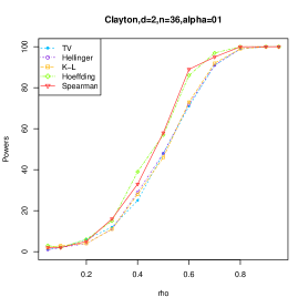
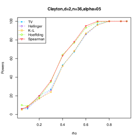
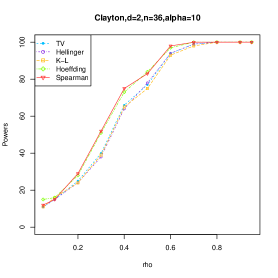
Another well known test for independence in the case is based on Spearman’s , and has been used extensively in applications. However, it is well known that this test has low power if the distribution under the alternative hypothesis is continuous but singular, as is the case for several copulas. We used a small value of the sample size, , to compare our results to those of other papers that also use small sample sizes in their simulations. We made use of the spearman.test function of the R package pspearman.
Figure 1 shows the power comparisons for the Clayton family. We observe that the power obtained by using the tests of Hoeffding, Blum-Kiefer-Rosenblatt and Spearman’s are slightly better at levels and than the ones we obtain using our statistics based on the total variation and Hellinger distances, and the Kullback-Leibler divergence. This behavior can also be observed for other standard Archimedean copulas such as Gumbel and Frank, among others. It is important to note that most of all these copulas are absolutely continuous, with complete support and with smooth densities. We did not use the supremum distance in the simulations because we observed a strong discretization effect on the distribution of the statistic (23) when the sample size is small. In other words, the different possible values of this statistic are very limited, leading to many ties in the simulated values.
It is not difficult to see, via simulations, that the independent tests of Hoeffding and Blum-Kiefer-Rosenblatt can also have problems with small sample sizes. In fact, we noted that when we sample from the independent copula , and test at the usual levels , the real levels of the test do not correspond to the desired values of . For example, if we set and perform several simulations, the actual value of under independence is approximately . Something similar happens with the other two values of . This is due to the discrete nature of the test statistic, and the problem is more severe when the sample size is small. For this reason, we recommend caution when using these two tests with small sample sizes.
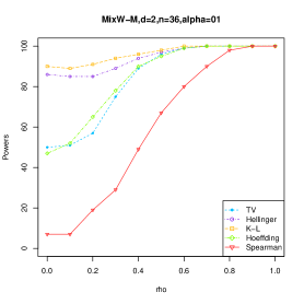
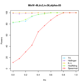
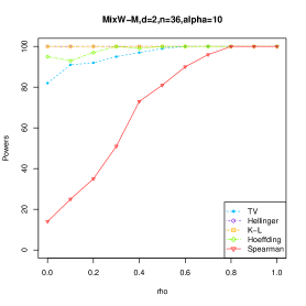
As a second example, we used the Fréchet-Mardia copulas. In this case, we use a convex mixture of and , the Fréchet-Hoeffding bounds. As we can see in Figure 2, the Spearman’s test has very low power, specially for singular copulas. We also note that the total variation statistic in equation (21) performs a little better than the Hoeffding and Blum-Kiefer-Rosenblatt tests at the three levels, but our test statistics based on the Hellinger distance and Kullback-Leibler divergence have the best performance at all three levels, and have a power close to 100% when and .
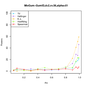
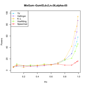
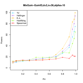
Finally, we used a convex combination of a Gumbel and a Gumbel-ID, where the latter denotes a Gumbel distribution with an increasing transformation in its first coordinate and a decreasing transformation in its second coordinate. That is, we applied the transformation to all the observations from the Gumbel copula. The notation ID stands for increasing-decreasing transformation. As we can see in Figure 3, in this case the Spearman’s , the Hoeffding and the Blum-Kiefer-Rosenblatt have lower powers than our three test statistics (21), (22) and (24). Moreover, the performance of these three statistics can be much better than the ones obtained using the standard tests. In particular, the Kulback-Leibler test (24) has the highest powers.
4.2 Dimension
Many of the test statistics proposed in dimension can be extended to higher dimensions. Some of these extensions are rather natural. For example, in the case of the Hoeffding statistic and dimension , we could use , where denotes the joint distribution function and , and are the margins of , and , respectively. If we now define , we could use the empirical version of to test for independence. The Blum-Kiefer-Rosenblatt statistic could be similarly extended. Many other test statistics based on the empirical copula have -dimensional versions, for example the statistic of Genest and Rémillard [7]. The problem with all these possible extensions is that in dimension the empirical copula may become difficult to compute if the sample size is not small. On the other hand, the use of the empirical distribution function in dimensions greater than or equal to requires large sample sizes in order to obtain reasonable approximations of the true distribution function. In the case of -copulas, the same is true of the empirical (sub)copula.
In some cases, one can find the asymptotic distribution of a test statistic based on the empirical distribution function or empirical copula, but this limiting distribution can only be reached with large sample sizes. In such cases, the test statistic may be difficult to evaluate, and so it would not be possible to assess for which sample sizes the limiting distribution actually provides a good approximation.
There are other tests, based on empirical processes or multivariate characteristic functions, which also have problems when working with large sample sizes; see, for example, [6]. In [2], the authors propose a statistic, , which coincides with the square product moment correlation when . The power of this test is adequate only for absolutely continuous random variables, and it has the same problem as Spearman’s test in dimension . On the other hand, in [21], the authors propose a new test of multivariate independence based on analogues of Kendall’s and Spearman’s . The comments of the previous paragraph also apply to these tests.
In the simulations using the four test statistics given by equations (21), (22), (23) and (24), we used relatively large values of the sample size . In many instances the other tests take a very long time. Therefore, we only have compared our proposals among themselves in order to see which one has better powers in a number of scenarios.
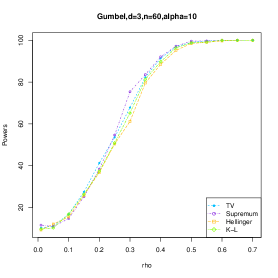
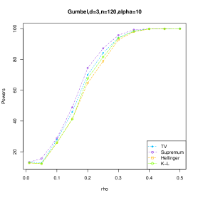
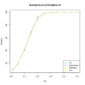
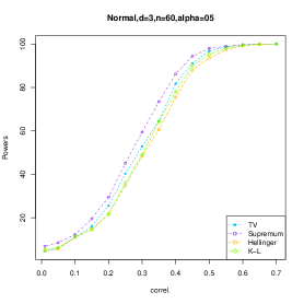
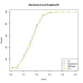
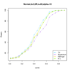
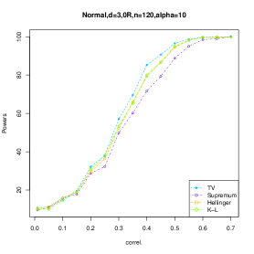
In Figures 4 through 6 we analyze the case . We used three sample sizes, , and , with simulations to find the critical values of the tests under . We also generated simulations under the alternative hypothesis, , to compute the powers of the four tests.
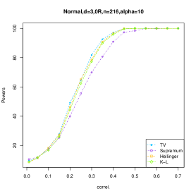
In Figure 4 we consider the Gumbel family, with . We observe that, for small , the test statistic based on the supremum distance has better powers, while for the powers are similar for all tests. As pointed out before, the statistic based on the supremum distance is highly discrete, which means that the critical values for this test are not very accurate. The same can be said about Figure 5, where we consider the normal family with a covariance matrix that has the same correlation for each pair of variables. We also note that the supremum distance has a little better power, but this advantage dissipates as the sample size increases. In Figure 6 we also study the normal family, but now one of the variables is independent of the other two. Note that in this case the test based on the supremum distance has the worst power compared to the other three statistics, but for large values of this difference seems to disappear.
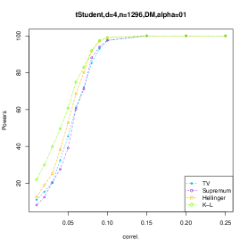
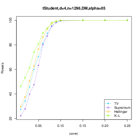
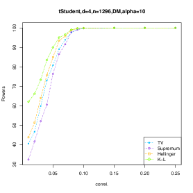
4.3 Dimension
The comments made for the case also apply to the case . The only difference is that here we consider different values of the sample size which now include and . (The value is obtained by multiplying the number of boxes of and in dimension .) It is worth emphasizing that, if we tried to evaluate the empirical distribution function of a sample of size in 4 dimensions, we would most likely get an error message because the array needed to store it would be of size , which no standard personal computer can handle.
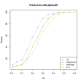
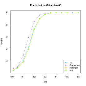
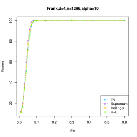
In Figure 7 we consider the Frank family with . The remarks for this case are similar to those relating to Figure 4. Finally, in Figure 8 we study the Student distribution with degrees of freedom and having the same correlation for all the pairs of variables. As is well known, this distribution has heavier tails than the normal distribution, and in this case the test based on the Kullback-Leibler divergence performs better than the other tests.
5 Real data example
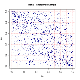
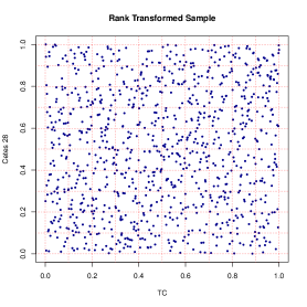
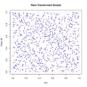
We applied our independence tests to real Mexican economic data in dimensions and . We used data recorded on consecutive days, from 2014 to 2017, concerning three variables: the USD/MXN Exchange Rate (Tipo de Cambio in Spanish, denoted here by TC); the Prices and Quotations Index of the Mexican Stock Exchange (Indice de Precios y Cotizaciones de la Bolsa Mexicana de Valores, denoted here by IPC); and the price of a Mexican bond known as Cetes 28, where 28 refers to days. As is common in financial contexts, we did not worked with the raw data but used the corresponding returns instead.
Figure 9 shows the scatter plots of the modified (rank transformed) returns for the pairs (TC,IPC), (TC,Cetes 28) and (IPC,Cetes 28). The corresponding values of the Pearson correlation coefficients are for (TC,IPC), for (TC,Cetes 28) and for (IPC,Cetes 28). When we applied our independence tests to the 3-dimensional data set, we rejected independence with all of them; that is, using the test statistics based on the total variation, supremum and Hellinger distances, as well as the Kullback-Leibler divergence.
We also applied our independence tests, together with Hoeffding, Blum-Kiefer-Rosenblatt and Spearman tests, to each of the three pairs of variables. For the first two pairs, (TC,IPC) and (TC,Cetes 28), all of the tests rejected independence at levels , and . However, for the pair (IPC, Cetes 28) none of the tests rejected independence at any of the three levels.
6 Discussion
In this paper we have provided a simple characterization of multivariate independence in terms of the checkerboard approximations of order 2 and 3 to a -variate copula. While interesting in its own right, this result has also allowed us to propose a new family of tests of multivariate independence for -variate continuous random vectors.
Our test statistics are all functionals of the sample copulas that estimate the above-mentioned checkerboard approximations. These estimators can be evaluated for relatively large sample sizes even if the dimension is not small. This allows us to produce a large number of simulations in order to estimate the null distributions of the statistics we propose. On the other hand, our test statistics can be defined in terms of any metric, or ever in terms of other functionals that are not symmetric such as the Kullback-Leibler divergence.
We simulated a range of examples in dimensions up to , under different models and with different sample sizes. In many of these scenarios, it may not be feasible to compute the empirical distribution functions. In our simulations we observed that, when the sample size is moderately large, all of the tests we considered have similar powers. Thus, in this case any of our test statistics may be used. However, when the sample size is small, we warn the user against the test statistic based on the supremum distance since it is strongly affected by discretization.
One interesting application of our tests is the following. Consider a random vector . In some cases it is possible to decompose into two independent subvectors and ; that is, we can find a permutation of and a value of such that the subvectors and are independent. Conversely, suppose there exist no permutation of and such that, for every ,
| (25) |
where and are marginal distribution functions. In this case we follow [12] and say that the random vector is exhaustively dependent.
In practice, it is not uncommon to find random vectors for which it can be assumed that a certain set of coordinates are independent from the remaining coordinates. In such cases, for a sample of size of this random vector, we would like to produce a statistical test for the independence of these two subvectors. In [12] the authors show that, if is a random vector on () with joint distribution function , and if there exists a permutation of such that all the subvectors , are dependent, then is exhaustively dependent.
Assume that and take to be the identity. Now let be a random vector such that and are two subvectors which are exhaustively dependent, and assume that we suspect that and are independent. If we have a random sample of size from the distribution of , we can verify all these assumptions using our tests of independence as follows. First, test if the subvectors for and for have independent coordinates (at a certain level for each test). If we reject the hypothesis of independence in all three tests, now we can test independence of the subvectors and by testing the independence between the coordinates of each of the following six subvectors: and . If we do not reject the hypothesis of independence for all these pairs, then we have some evidence that our assumptions are not incorrect. Note that in this case all the independence tests are performed for pairs of random variables, which makes the tests quite quick even for large sample sizes.
We have developed a program in the statistical language R that implements the procedure described above. The code is available from the authors upon request.
Appendix
Proof of Theorem 2.4
First, assume that . Let us assume that , that is, is the independence copula; then, using equation (4), we have
is a 2-subcopula. For this 2-subcopula and the uniform partition of size given in equation (3), and using equation (1), we have that for every ,
| (26) | |||||
where is the Lebesgue measure on .
If we use the bilinear interpolation of Lemma 2.3.5 in Nelsen’s book, see [18], we have that the checkerboard approximation of order of has a density given by equation (5)
for every . Hence, the density of is the constant on . Therefore, for every integer , the checkerboard approximation satisfies
| (28) |
In particular this holds for and .
Now, let us assume that for some 2-copula we have that for every . Let and define , as in the uniform partition of order , given in equation (3). Then, by equation (1) and using inequality (2), if , we have
| (29) |
Note that is a disjoint union. Note also that, by continuity of , ; the same applies to and . Hence, using equation (1),
and so . Similar arguments show that and that . So, using the bilinear interpolation we obtain
From equation (Proof of Theorem 2.4) we have that is a function of a unique parameter, that is, , and from the hypothesis we have that , where from equation (29), .
Now, we also assume that satisfies
| (30) |
for every . In order to construct we need to evaluate all the volumes for every . We first observe that , so using equation (Proof of Theorem 2.4), we obtain
| (31) |
In general, by continuity of , for every . We also know from equation (3), that for every . Hence, using equation (27), the density of is given by
| (32) |
for every and for every . Using equations (Proof of Theorem 2.4) and (31) we have that
| (33) |
for every . We also have that
| (34) | |||||
Now, using equations(33), (34) and integration we obtain
| (35) |
for every .
Finally, let us take . Using equation (3), we have that , while from equation (Proof of Theorem 2.4) we have
| (36) |
On the other hand, from equations (34) and (35) it follows that
| (37) |
Therefore, from hypothesis (30) and equations (36) and (37), we have that
However, by equation (Proof of Theorem 2.4), this happens if and only if .
We now assume that and that is the product 3-copula. Then using equation (4) we know that
is a 3-subcopula, and for this 3-subcopula and the uniform partition of size given in equation (3), and using equation (1), we have by continuity of that
| (38) | |||||
where is the Lebesgue measure on .
If we use the trilinear interpolation of Lemma 2.3.5 in Nelsen’s book, [18], we have that the checkerboard approximation of order of has a density given by equation (5)
| (39) |
for every . Hence, the density of is the constant on . Therefore, for every integer the checkerboard approximation satisfies that
| (40) |
In particular this holds for and .
We now prove the converse. Let us assume that for some 3-copula we have that for every . Let and define as in the uniform partition of order given in equation (3). Then, by equation (1), ; using now the inequality (2), we have
| (41) |
Define and . Let , the we know that is a 2-copula, and by hypotheses we also know that for every . It is trivial to see that by linearity in the construction of and , we have that the checkerboards of of order and are given by and for every . Therefore, we have the transformed hypotheses
| (42) |
So, using what we proved in the case above,
| (43) |
Defining and for every , and reasoning as above we observe that
| (44) |
Now using the fact that any 3-copula is increasing in each coordinate, together with equations (43) and (44) and inequality (41) we have
| (45) |
In order to find , we need first to evaluate the -volumes of all the uniform boxes for every , in order to find its density in each box, which is given by the constant for every . We know that . By equation (1) and using i) in Definition 2.1, we have that , similarly . Again, by equation (1) and using i) and ii) in Definition 2.1, we obtain , analogously, . Finally, using Definition 2.1 we have that .
Therefore, integrating the above density we get the checkerboard copula of order , for every , which is given by:
Note that by hypothesis , and that by equation (Proof of Theorem 2.4) it has a unique parameter .
In order to obtain , we will obtain its density using equation (Proof of Theorem 2.4), that is,
| (46) |
for every and for every , as defined in equation (3). To find the density of on we observe that , so, using (Proof of Theorem 2.4), . To obtain the density of on , we need . For the density of on we need . Finally, for the density of on we need . Hence, from equation (46), we have that has density on and , and density on .
Now let , Then, by hypothesis, . Integrating the density of we have
| (47) | |||||
and using equation (Proof of Theorem 2.4) we know that . Therefore,
Solving for we have that , and using equation (Proof of Theorem 2.4), we have that for every . The rest of the proof follows by induction.
References
- [1] Bagkavos, D. and Patil, P.N. (2017). A new test of independence for bivariate observations. J. Multivariate Anal., 160, 117-133.
- [2] Bakirov, N.K., Rizzo, M.L. and Székely, G.J. (2006). A multivariate nonparametric test of independence. J. Multivariate Anal., 97, 1742–1756.
- [3] Blum, J.R., Kiefer, J. and Rosenblatt, M. (1961). Distribution free tests of independence based on the sample distribution function. Ann. Math. Statist., 32, 485–498.
- [4] Cuberos, A., Masiello, E. and Maume-Deschamps, V. (2016). Copulas checker-type approximations: applications to quantiles estimation of aggregated variables. hal-012201838v2.
- [5] Durante, F. and Fernández-Sánchez, J. (2010). Multivariate shuffles and approximations of copulas. Statist. Probab. Lett., 80, 1827–1834.
- [6] Fan, Y., Lafaye de Micheaux, P., Penev, S. and Salopek, D. (2017). Multivariate nonparametric test of independence. J. Multivariate Anal., 153, 189–210.0
- [7] Genest, C. and Rémillard, B. (2004). Tests of independence and randomness based on the empirical copula process. TEST, 13, 335-369.
- [8] Gibbs, A.L. and Su, F.E. (2002). On choosing and bounding probability metrics. arXiv:math/020902v1[math.PR]3Sep2002, 1–21.
- [9] González-Barrios, J.M. and Hernández-Cedillo, M.M. (2013). Sample -copula of order . Kybernetika, 49, 663–669.
- [10] González-Barrios, J.M. and Hoyos-Argüelles, R. (2018a). Distributions associated to the counting techniques of the -sample copula of order and weak convergence of the sample process. Comm. Statist. Simulation Comput. In press, DOI:101080/036/0918.2018.1520874.
- [11] González-Barrios, J.M. and Hoyos-Argüelles, R. (2018b). Estimating checkerboard approximations with sample -copulas. Submitted.
- [12] González-Barrios, J.M., Gutiérrez-Peña, E. and Rueda, R. (2019). A short note on the dependence structure of random vectors. Statist. Probab. Lett., 146, 200–205.
- [13] Hoeffding, W. (1948). A nonparametric test of independence. Ann. Math. Statist., 19, 546–557.
- [14] Jansen, P., Swanepoel, J. and Veraverbeke, N. (2012). Large sample behavior of the Bernstein copula estimator. J. Statist. Plann. Inference, 142, 1189-1197.
- [15] Li, X., Mikusiński, P. and Taylor, M.D. (1998). Strong approximations of copulas. J. Math. Anal. Appl., 225, 608–623.
- [16] Mikusiński, P. and Taylor, M.D. (2010). Some approximations of -copulas. Metrika, 72, 385–414.
- [17] Mudholkar, G.S. and Wilding, G.E. (2005). Two Wilson-Hilfetry type approximations for the null distribution of the Blum, Kiefer and Rosenblatt test of bivariate independence. J. Statist. Plann. Inference, 128, 31–41.
- [18] Nelsen, R.B. (2006). An introduction to copulas. 2nd ed., Lect. Notes in Statist., Springer-Verlag, New York.
-
[19]
R Core Team (2017). R: A language and environment for statistical
computing. R Foundation for Statistical Computing, Vienna, Austria.
URL
https://www.R-project.org/. - [20] Segers, J., Sibuya, M. and Tsukahara, H. (2017). The empirical beta copula. J. Multivariate Anal., 155, 35–51.
- [21] Taskinen, S., Randles, R.H. and Oja, H. (2005). Multivariate nonparametric tests of independence. J. Amer. Statist. Assoc., 100, (471), 916–925.