A Low-Rank Schwarz Method for Radiative Transfer Equation with Heterogeneous Scattering Coefficientthanks: The work of JL is supported in part by the National Science Foundation via grant DMS-1454939. The work of KC, QL, and SW is supported in part by the National Science Foundation via grant 1740707. The work of SW is further supported in part by National Science Foundation grants 1628384 and 1634597; Subcontract 8F-30039 from Argonne National Laboratory; and Award N660011824020 from the DARPA Lagrange Program. The work of KC and QL is further supported in part by Wisconsin Data Science Initiative and National Science Foundation via grant DMS-1750488, and DMS-1107291: RNMS KI-Net.

Ke Chen Mathematics Department, University of Wisconsin-Madison, Madison, WI 53706 (kchen222@wisc.edu)    Qin Li Mathematics Department and Discovery Institute, University of Wisconsin-Madison, Madison, WI 53706 (qinli@math.wisc.edu)    Jianfeng Lu Department of Mathematics, Department of Physics, and Department of Chemistry, Duke University, Durham, NC 27708 (jianfeng@math.duke.edu)    Stephen J. Wright Computer Sciences Department, University of Wisconsin, Madison, WI 53706 (swright@cs.wisc.edu)
Abstract

Random sampling has been used to find low-rank structure and to build fast direct solvers for multiscale partial differential equations of various types. In this work, we design an accelerated Schwarz method for radiative transfer equations that makes use of approximate local solution maps constructed offline via a random sampling strategy. Numerical examples demonstrate the accuracy, robustness, and efficiency of the proposed approach.

keywords:
Random sampling, Schwarz method, heterogeneous media, radiative transfer equation
AMS:
65N

1 Introduction

The radiative transfer equation (RTE) is a standard model that describes propagation of light through such turbid media as biological tissues or planetary atmospheres. The equation is used in situations in which energy is transported by light, as in the study of the greenhouse effect [4], optical tomography [28], and the radiation field for atmosphere-ocean system [38]. Light is injected from a source, and RTE models the absorption and scattering of the photons in the ambient material.

The model equation for the steady state is

vxu(x,v)=σ(x)u(x,v),(x,v)𝒟:=𝒦×𝒱,formulae-sequence𝑣subscript𝑥𝑢𝑥𝑣𝜎𝑥𝑢𝑥𝑣𝑥𝑣𝒟assign𝒦𝒱v\cdot\nabla_{x}u(x,v)=\sigma(x)\mathcal{L}u(x,v)\,,\quad(x,v)\in\mathscr{D}:=\mathcal{K}\times\mathcal{V}, (1)

where u(x,v)𝑢𝑥𝑣u(x,v) describes the light intensity at location x𝑥x oriented in velocity direction v𝑣v. The left-hand side describes free propagation of the photons along direction x𝑥x with velocity v𝑣v, while the right-hand side characterizes interaction between photons and media (via absorption and scattering). The media information is encoded in σ(x)𝜎𝑥\sigma(x), which is strictly positive for all x𝑥x. The operator \mathcal{L}, typically an integral operator, characterizes how photons are scattered and change directions. We denote the physical domain by 𝒦𝒦\mathcal{K}. Since photons always move with the same speed, the velocity term is determined purely by the direction, so that v𝒱=𝕊d1𝑣𝒱superscript𝕊𝑑1v\in\mathcal{V}=\mathbb{S}^{d-1}, the unit sphere in d𝑑d dimensions.

In the large space-regime, with scaling xxε𝑥𝑥𝜀x\to\frac{x}{\varepsilon} (where ε𝜀\varepsilon is a small parameter discussed below), the equation (1) becomes

εvxu(x,v)=σδ(x)u(x,v),𝜀𝑣subscript𝑥𝑢𝑥𝑣superscript𝜎𝛿𝑥𝑢𝑥𝑣\varepsilon v\cdot\nabla_{x}u(x,v)=\sigma^{\delta}(x)\mathcal{L}u(x,v)\,, (2)

where σδ(x)superscript𝜎𝛿𝑥\sigma^{\delta}(x) is the rescaled media function, with δ𝛿\delta capturing the smallest scale of the variation in the media. This function is rough when δ1much-less-than𝛿1\delta\ll 1. In the equation (2), ε𝜀\varepsilon is the Knudsen number that represents the ratio of the mean free path to the typical domain length.

With appropriate boundary conditions, well-posedness of the equation is straightforward, and is independent of the scales (that is, the smallness of ε𝜀\varepsilon or δ𝛿\delta[2, 14]. In this paper, we tackle the numerical challenge of designing an efficient numerical solver for (2). We are especially interested in the regime of small ε𝜀\varepsilon and small δ𝛿\delta, where classical numerical methods typically require high memory and computational cost, as we explain below.

1.1 Asymptotic preserving

Small parameters in PDEs can induce computational challenges. In the case described above, we have xu1/min{ε,δ}similar-tosubscript𝑥𝑢1𝜀𝛿\nabla_{x}u\sim{1}/{\min\{\varepsilon\,,\delta\}}, so a classical numerical solver can be expected to attain good accuracy only when the mesh size in the discretization ΔxΔ𝑥\Delta x satisfies

Δxmin{ε,δ}.much-less-thanΔ𝑥𝜀𝛿\Delta x\ll\min\{\varepsilon\,,\delta\}\,.

A grid in d𝑑d dimensions with this discretization parameter will have at least Nmin(ε,δ)dN\gg\min(\varepsilon,\delta)^{-d} grid points, so the computation is prohibitive when ε𝜀\varepsilon and δ𝛿\delta are small.

A natural question is whether it is possible to design a numerical method for which the computational cost of obtaining a stable, accurate solution is independent of the parameters ε𝜀\varepsilon and δ𝛿\delta, and whether the numerical solution can capture the right asymptotic limit of the solution as ε𝜀\varepsilon and δ𝛿\delta approach zero. If a numerical solver for a multiscale problem has its discretization independent of the smallest scale in the equation, but still preserves the asymptotic limits, then the solver is called asymptotic-preserving (AP). This term was coined in [26] for a class of kinetic equations, although some algorithms for simpler settings had been designed previously [30]. Extensive progress has been made during the past decade, with AP solvers being designed for the Bhatnagar-Gross-Krook equation (BGK, a special simplified version of the Boltzmann model that keeps the equilibrium), the Boltzmann equation, the Vlasov-Poisson-Boltzmann (VPB) equation, and many others [31, 13, 16, 15, 25]. See also the reviews [27].

A standard approach for designing AP solvers is based on analysis of the asymptotic limits. In some cases, asymptotic limits for the equations can be derived: the Euler limit for the Boltzmann, the coupled diffusion-Poisson system for the VPB system. One strategy for obtaining the AP property is to work with two sets of solvers, one for the original equation and one for the asymptotic limit, the latter being encoded in the former via a weight that can be tuned. In the limit as ε0𝜀0\varepsilon\to 0, this weight is adjusted so that the limiting equation solver dominates, driving the numerical solution to that of the asymptotic limiting system.

The analysis-based approach is straightforward and mathematically sound, and has made some previously impossible computations feasible. It depends, however, on analytical understanding of the asymptotic limit, which is not always straightforward. We are led to ask whether it is possible to design an AP solver that does not require detailed knowledge of the asymptotic limit. This paper addresses this question in the specific case of RTE. This equation is complicated in that different patterns of convergence of the pair (ε,δ)𝜀𝛿(\varepsilon,\delta) to (0,0)00(0,0) lead to different limiting systems, not all of which are well understood. Can we design AP numerical solvers in the absence of this analytical understanding? We outline an answer to this question in the next section.

1.2 Random Sampling and PDE Compression

We design AP solvers without analytical knowledge by using compression techniques. Even when asymptotic limits of equations with small parameters are difficult to derive analytically, we can sometimes show the existence of such limits. In the discrete setting, a basic second order discretization scheme with Δx=o(τϵ,τδ)Δ𝑥𝑜𝜏italic-ϵ𝜏𝛿\Delta x=o(\sqrt{\tau}\epsilon,\sqrt{\tau}\delta) should suffice to attain the accuracy level τ𝜏\tau, which leads to Nε=min{ετ,δτ}dN_{\varepsilon}=\min\{{\varepsilon\sqrt{\tau}},\delta\sqrt{\tau}\}^{-d} grid points for O(1)𝑂1O(1) domain-size. When a limiting equation exists, this accuracy level may be attainable with as few as N=τd𝑁superscript𝜏𝑑N=\tau^{-d} grid points. Since the limiting equation is asymptotically close to the original equation, these N𝑁N degrees of freedom are asymptotically sufficient to represent the original PDE solution that naively would require Nεsubscript𝑁𝜀N_{\varepsilon} grid points to compute. This observation implies that the Nεsubscript𝑁𝜀N_{\varepsilon}-dimensional solution space is compressible, and can be well approximated by a N𝑁N-dimensional space when ε𝜀\varepsilon and δ𝛿\delta are small.

Knowing that the space is “compressible”, can one find the compressed space quickly? We answer this question affirmatively, in the case of the RTE, by making use of random sampling. Random sampling is not a new strategy. It has been used in data science to sample sparse vectors (as in compressed sensing [9]) and low-rank matrices [23], with the goal of reconstructing these objects from a relatively small number of samples. Generally, the number of samples is tied more closely to the intrinsic dimension of the object (for example, the number of non-zeros in a sparse vector) than to the dimension of the ambient space, which is typically much larger.

Applications of random sampling techniques to PDEs have been limited previously to the discrete algebraic systems obtained by discretizing the PDEs. A direct link to the original PDEs needs to be explored further. Some important questions have not been fully resolved, for example, whether the PDE solution space or the solution operator is “compressible”. The two views correspond to regarding a matrix as defining a column space or as a linear operator, respectively. Other questions involve the sense in which these objects are “compressible”, and whether the spectral norm used for matrices is the appropriate norm in the case of PDEs.

Previously, mostly in the context of elliptic PDEs, the low rank property of the solution space has been investigated and utilized in numerical solvers. For example, homogenization theory has been utilized [24, 37] for designing local basis functions for multiscale problems with structured media. For more general setting of Lsubscript𝐿L_{\infty} media, the Kolmogorov N𝑁N-width or the problem was studied in a pioneering paper [3], while the structure fo the Green’s functions were investigated in the framework of hierarchical matrix [6, 22]. Inspired by the studies, many algorithms have been proposed to utilize the rank (or decay) property, including [12, 35, 29]. Algorithms that specifically use PDE compression and random sampling ideas are developed in [8, 39, 36, 7, 17]. In the transport equation setting, [11] incorporated the random sampling technique within the discontinuous Galerkin framework for building local solution dictionaries. Corresponding to the first question asked above, in most of these papers, the authors regard the solution space to be “compressible” and the associated matrix is regarded as a column space. A more systematic investigation of PDE compression appears recently in our previous work [10], where compressed PDE solution spaces are related to low rank structure of the matrix formed by the Green’s functions. Such concepts in multi-scale PDE computation as asymptotic-preserving (see above) and numerical homogenization are unified under this framework.

1.3 Contribution

This paper follows the line of research started in [10]. For RTE (2), we know only that the equation has asymptotic limits with small parameters, but the actual forms of the limiting equations are unknown. We aim to design an accurate numerical scheme whose runtime is independent of the smallness of the coefficients in the equation.

We apply the Schwarz iteration under the domain decomposition framework. The domain is divided into overlapping subdomains (patches). The PDEs in these patches can be solved in parallel. Solution of the PDE on each patch with partial boundary conditions yields an output in the form of boundary conditions that are passed to neighboring patches. The PDE on each patch is solved again with the modified boundary conditions supplied by its neighbors, the whole process repeating until the solutions are consistent in the overlapping regions. The boundary-to-boundary map, in which the inputs are the partial boundary conditions on the patch PDEs and the output are the missing boundary conditions obtained by solving the PDEs, is a compressible map. We will develop an algorithm based on random sampling that computes an adequate approximation to this map quickly. The overall scheme is a composition of an offline component, in which low-rank approximations to the boundary-to-boundary maps are obtained using random sampling; and an online step, in which Schwarz iteration, accelerated by the low-rank boundary-to-boundary map, is executed until a solution consistent across the whole domain is found.

Our work contrasts with the approach in [10], where the local solution space is compressed in an offline step. In the online step, a solution for particular boundary conditions or source term is found as a linear combination of basis vectors for the compressed space, with the coefficients chosen to match the given conditions. The problem of finding these coefficients is typically overdetermined, the number of coefficients being fewer than the constraints arising from the boundary conditions or source term. Some accuracy is sacrificed, and the error is difficult to quantify. The current work compresses the boundary-to-boundary map, rather than the local solution space, in the offline stage, and uses the compressed map to update local boundary conditions in the online stage, until a preset error tolerance is achieved.

In this work, to demonstrate our numerical scheme and validate our theory, we consider a simpler setting of 1+1111+1 problem, that is, one spatial dimension and one velocity dimension. Our theory can be extended to higher dimensions in a conceptually straightforward way, but the implementation of the numerical scheme would become significantly more delicate in such cases. We do not pursue high-dimensional versions in this paper.

The remainder of the paper is organized as follows. We introduce the concept of “low-rankness” in the context of the RTE in Section 2. In Section 3, we review the Schwarz iteration under the domain decomposition framework, and present the new low-rank Schwarz iteration method based on random sampling. Numerical experience is described in Section 4.

2 Low-rankness of RTE in Various Regimes

As discussed above, current AP schemes rely heavily on good understanding of the analytical form of the asymptotic limits, although in some situations, this limiting form is hard to specify, even when we know that it exists. The radiative transfer equation with small Knudsen number ε𝜀\varepsilon and small media oscillation period δ𝛿\delta is a good example of the latter phenomenon. As ε𝜀\varepsilon and δ𝛿\delta converge to (0,0)00(0,0) in different ways, the limiting equations are different, and only some of the limiting forms can be expressed explicitly. We show two different homogenization effects in the following two subsections, and unify them using the concept of the low-rankness in Section 2.3.

Consider the RTE in infinite domain (2), which we restate here:

εvxu(x,v)=σδ(x)u(x,v),𝜀𝑣subscript𝑥𝑢𝑥𝑣superscript𝜎𝛿𝑥𝑢𝑥𝑣\varepsilon v\cdot\nabla_{x}u(x,v)=\sigma^{\delta}(x)\mathcal{L}u(x,v), (3)

where xd𝑥superscript𝑑x\in\mathbb{R}^{d} and v𝒱=𝕊d1𝑣𝒱superscript𝕊𝑑1v\in\mathcal{V}=\mathbb{S}^{d-1}. We define the scattering operator \mathcal{L} to have the following form:

u(x,v)=𝕊d1u(x,v)dμ(v)u(x,v),𝑢𝑥𝑣subscriptsuperscript𝕊𝑑1𝑢𝑥superscript𝑣differential-d𝜇superscript𝑣𝑢𝑥𝑣\mathcal{L}u(x,v)=\int_{\mathbb{S}^{d-1}}u(x,v^{\prime})\,\mathrm{d}\mu(v^{\prime})-u(x,v)\,,

where μ(v)𝜇𝑣\mu(v) is the normalized measure on the velocity domain. The scattering coefficient σδ(x)>0superscript𝜎𝛿𝑥0\sigma^{\delta}(x)>0 encodes the media information, with δ𝛿\delta denoting the smallest spatial scale. The operator has a nontrivial null space Null Null \text{Null\,}\mathcal{L} which consists of functions that are constant in the velocity domain. We use this fact later to formally derive the diffusion limit of RTE. In this article, we choose the operator \mathcal{L} to have this specific form, for simplicity. In practice, especially in applications to atmosphere science, the radiative transfer equation often takes this operator to be u(x,v)=𝕊d1k(x,v,v)u(x,v)dμ(v)σ(x,v)u(x,v)𝑢𝑥𝑣subscriptsuperscript𝕊𝑑1𝑘𝑥𝑣superscript𝑣𝑢𝑥superscript𝑣differential-d𝜇superscript𝑣𝜎𝑥𝑣𝑢𝑥𝑣\mathcal{L}u(x,v)=\int_{\mathbb{S}^{d-1}}k(x,v,v^{\prime})u(x,v^{\prime})\,\mathrm{d}\mu(v^{\prime})-\sigma(x,v)u(x,v) with the collision kernel

k(x,v,v)=1g24π(1+g22gvv)3/2,𝑘𝑥𝑣superscript𝑣1superscript𝑔24𝜋superscript1superscript𝑔22𝑔𝑣superscript𝑣32k(x,v,v^{\prime})=\frac{1-g^{2}}{4\pi(1+g^{2}-2gv\cdot v^{\prime})^{3/2}}\,,

where the constant g[1,1]𝑔11g\in[-1,1] determines the relative strength of the forward and backward scattering. This is the so-called Henyey-Greenstein model. The equation would have the same type of asymptotic limit (an elliptic equation) as long as σ(x,v)=k(x,v,v)dμ(v)𝜎𝑥𝑣𝑘𝑥𝑣superscript𝑣differential-d𝜇superscript𝑣\sigma(x,v)=\int k(x,v,v^{\prime})\mathrm{d}\mu(v^{\prime}) [2, 14].

We now consider different limits for different regimes of the parameters (ε,δ)𝜀𝛿(\varepsilon,\delta).

2.1 Diffusion Regime

In the diffusion regime, we have ε0𝜀0\varepsilon\to 0 while δ𝛿\delta is fixed at a positive value. From (3), we see that u(x,v)0similar-to𝑢𝑥𝑣0\mathcal{L}u(x,v)\sim 0 in the leading order, meaning that u(x,v)𝑢𝑥𝑣u(x,v) belongs to the null space of \mathcal{L}, and loses its velocity dependence. By matching orders in the classical asymptotic expansion

u(x,v)=u0(x,v)+εu1(x,v)+,𝑢𝑥𝑣subscript𝑢0𝑥𝑣𝜀subscript𝑢1𝑥𝑣u(x,v)=u_{0}(x,v)+\varepsilon u_{1}(x,v)+\cdots\,,

we obtain

𝒪(1)::𝒪1absent\displaystyle\mathcal{O}(1): u0(x,v)Null,subscript𝑢0𝑥𝑣Null\displaystyle\quad u_{0}(x,v)\in\text{Null}\mathcal{L}\,,\quad u0(x,v)=u0(x),subscript𝑢0𝑥𝑣subscript𝑢0𝑥\displaystyle u_{0}(x,v)=u_{0}(x)\,,
𝒪(ε)::𝒪𝜀absent\displaystyle\mathcal{O}(\varepsilon): vxu0(x,v)=σδu1,𝑣subscript𝑥subscript𝑢0𝑥𝑣superscript𝜎𝛿subscript𝑢1\displaystyle\quad v\cdot\nabla_{x}u_{0}(x,v)=\sigma^{\delta}\mathcal{L}u_{1}\,,\quad u1(x,v)=1σδvxu0(x),subscript𝑢1𝑥𝑣1superscript𝜎𝛿𝑣subscript𝑥subscript𝑢0𝑥\displaystyle u_{1}(x,v)=-\frac{1}{\sigma^{\delta}}v\cdot\nabla_{x}u_{0}(x)\,,
𝒪(ε2)::𝒪superscript𝜀2absent\displaystyle\mathcal{O}(\varepsilon^{2}): vxu1(x,v)=σδu2,𝑣subscript𝑥subscript𝑢1𝑥𝑣superscript𝜎𝛿subscript𝑢2\displaystyle\quad v\cdot\nabla_{x}u_{1}(x,v)=\sigma^{\delta}\mathcal{L}u_{2}\,,\quad vxu1(x,v)dμ(v)=0.𝑣subscript𝑥subscript𝑢1𝑥𝑣differential-d𝜇𝑣0\displaystyle\smallint v\cdot\nabla_{x}u_{1}(x,v)\mathrm{d}\mu{(v)}=0\,.

By substituting the 𝒪(ε)𝒪𝜀\mathcal{O}(\varepsilon) equation into the 𝒪(ε2)𝒪superscript𝜀2\mathcal{O}(\varepsilon^{2}) equation, one obtains a diffusion equation, as follows.

Theorem 1 ([5]).

In the zero limit of ε𝜀\varepsilon, the solution to (3) converges to the solution to the diffusion equation:

x(1σδ(x)xu0(x))=0,subscript𝑥1superscript𝜎𝛿𝑥subscript𝑥subscript𝑢0𝑥0\nabla_{x}\cdot\left(\frac{1}{\sigma^{\delta}(x)}\nabla_{x}u_{0}(x)\right)=0\,, (4)

in the sense that

u(x,v)u0(x)L2(dxdμ(v))=𝒪(ε).subscriptnorm𝑢𝑥𝑣subscript𝑢0𝑥subscript𝐿2d𝑥d𝜇𝑣𝒪𝜀\|u(x,v)-u_{0}(x)\|_{L_{2}(\mathrm{d}x\,\mathrm{d}\mu(v))}=\mathcal{O}(\varepsilon)\,.
Remark 2.

Note that we did not account for boundary conditions in deriving the limiting equation. In physical space, the derivation is valid when the boundary conditions are periodic. Otherwise, one has to be careful with the boundary influences and curvature effects. The diffusion limit still holds outside the boundary layers, but the convergence deteriorates when curvature corrections need to be taken into account. These results can be found in [21, 33] for the case when domain is convex.

2.2 Homogenization Regime

When ε𝜀\varepsilon is fixed at a positive value while δ0𝛿0\delta\to 0, homogenization limits are achieved; see [18]. We assume a two-scale media, having dependence on a fast variable y=xδ𝑦𝑥𝛿y=\frac{x}{\delta} and a slow variable x𝑥x:

σδ(x)=σ(x,xδ),superscript𝜎𝛿𝑥𝜎𝑥𝑥𝛿\sigma^{\delta}(x)=\sigma\left(x,\frac{x}{\delta}\right),

where σ(x,)𝜎𝑥\sigma(x,\cdot) is assumed to be periodic (with respect to the fast variable) for each x𝑥x. Accordingly, we write the solution as

uδ(x,v)=u(x,y,v)=u(x,xδ,v).superscript𝑢𝛿𝑥𝑣𝑢𝑥𝑦𝑣𝑢𝑥𝑥𝛿𝑣u^{\delta}(x,v)=u(x,y,v)=u\left(x,\frac{x}{\delta},v\right).

In this notation, the operator xsubscript𝑥\nabla_{x} is replaced by x+1δysubscript𝑥1𝛿subscript𝑦\nabla_{x}+\frac{1}{\delta}\nabla_{y} from chain rule. By substituting into the equation, we have

vxuδ(x,y,v)+1δvyuδ(x,y,v)=σ(x,y)εuδ.𝑣subscript𝑥superscript𝑢𝛿𝑥𝑦𝑣1𝛿𝑣subscript𝑦superscript𝑢𝛿𝑥𝑦𝑣𝜎𝑥𝑦𝜀superscript𝑢𝛿v\cdot\nabla_{x}u^{\delta}(x,y,v)+\frac{1}{\delta}v\cdot\nabla_{y}u^{\delta}(x,y,v)=\frac{\sigma(x,y)}{\varepsilon}\mathcal{L}u^{\delta}\,.

By substituting the asymptotic expansion

uδ(x,y,v)=u0(x,y,v)+δu1(x,y,v)+𝒪(δ2),superscript𝑢𝛿𝑥𝑦𝑣subscript𝑢0𝑥𝑦𝑣𝛿subscript𝑢1𝑥𝑦𝑣𝒪superscript𝛿2u^{\delta}(x,y,v)=u_{0}(x,y,v)+\delta u_{1}(x,y,v)+\mathcal{O}(\delta^{2})\,,

into the equation above, and matching terms, we obtain

𝒪(1/δ)::𝒪1𝛿absent\displaystyle\mathcal{O}(1/\delta): vyu0(x,y,v)𝑣subscript𝑦subscript𝑢0𝑥𝑦𝑣\displaystyle v\cdot\nabla_{y}u_{0}(x,y,v) =0,absent0\displaystyle=0\,, (5a)
𝒪(1)::𝒪1absent\displaystyle\mathcal{O}(1): vxu0σ(x,y)εu0𝑣subscript𝑥subscript𝑢0𝜎𝑥𝑦𝜀subscript𝑢0\displaystyle v\cdot\nabla_{x}u_{0}-\frac{\sigma(x,y)}{\varepsilon}\mathcal{L}u_{0} =vyu1(x,y,v).absent𝑣subscript𝑦subscript𝑢1𝑥𝑦𝑣\displaystyle=v\cdot\nabla_{y}u_{1}(x,y,v)\,. (5b)

By applying the Fourier transform for the first equation (5a) with respect to the periodic variable y𝑦y, we obtain

i2πvξu^0(x,ξ,v)=0,for all ξd.𝑖2𝜋𝑣𝜉subscript^𝑢0𝑥𝜉𝑣0for all ξd.i2\pi v\cdot\xi\hat{u}_{0}(x,\xi,v)=0\,,\quad\mbox{for all $\xi\in\mathbb{Z}^{d}$.}

We note that for almost all fixed vd𝑣superscript𝑑v\in\mathbb{R}^{d}, the multiplier i2πvξ𝑖2𝜋𝑣𝜉i2\pi v\cdot\xi is non-vanishing for all ξd\{0}𝜉\superscript𝑑0\xi\in\mathbb{Z}^{d}\backslash\{0\}, because otherwise there exists some ξd\{0}𝜉\superscript𝑑0\xi\in\mathbb{Z}^{d}\backslash\{0\} such that i2πvξ=0𝑖2𝜋𝑣𝜉0i2\pi v\cdot\xi=0 for a positive measure set of v𝑣v, which is impossible. Therefore, by dividing the multiplier, we have for any ξd\{0}𝜉\superscript𝑑0\xi\in\mathbb{Z}^{d}\backslash\{0\} that

u^0(x,ξ,v)=0,for almost all (x,v).subscript^𝑢0𝑥𝜉𝑣0for almost all 𝑥𝑣\hat{u}_{0}(x,\xi,v)=0\,,\quad\text{for almost all }(x,v)\,.

That is, all Fourier modes are vanishing except for the one with ξ=0𝜉0\xi=0. This implies that u0subscript𝑢0u_{0} is independent of the periodic variable y𝑦y, so we redefine the notation to omit this dependence:

u0(x,y,v)=u0(x,v),for almost all (x,v).subscript𝑢0𝑥𝑦𝑣subscript𝑢0𝑥𝑣for almost all 𝑥𝑣\quad u_{0}(x,y,v)=u_{0}(x,v)\,,\quad\text{for almost all }(x,v)\,.

For the next order equation (5b), when we take the integral over y𝑦y, the RHS vanishes due to periodicity, and we obtain the homogenized equation

vxu0(x,v)=σ(x)εu0(x,v),withσ=σ(x,y)dy.formulae-sequence𝑣subscript𝑥subscript𝑢0𝑥𝑣superscript𝜎𝑥𝜀subscript𝑢0𝑥𝑣withsuperscript𝜎𝜎𝑥𝑦differential-d𝑦v\cdot\nabla_{x}u_{0}(x,v)=\frac{\sigma^{\ast}(x)}{\varepsilon}\mathcal{L}u_{0}(x,v)\,,\quad\text{with}\quad\sigma^{\ast}=\smallint\sigma(x,y)\mathrm{d}{y}\,.

The derivation of homogenization limit presented above is validated in the following theorem. See [18, Theorem 3.1] for a rigorous proof for the time-dependent case.

Theorem 3.

Let σδ(x)superscript𝜎𝛿𝑥\sigma^{\delta}(x) be a bounded family of Lsuperscript𝐿L^{\infty} functions such that

σδδ0σ,inLweak-topology,𝛿0superscript𝜎𝛿superscript𝜎insuperscript𝐿weak-topology\sigma^{\delta}\xrightarrow{\delta\rightarrow 0}\sigma^{\ast}\,,\quad\text{in}\ L^{\infty}\ \text{weak-}\ast\,\text{topology},

then the solution uδ(x,v)superscript𝑢𝛿𝑥𝑣u^{\delta}(x,v) to the RTE (3) (with ε𝜀\varepsilon fixed) converges in Lsuperscript𝐿L^{\infty} weak-\ast topology to u(x,v)𝑢𝑥𝑣u(x,v), the solution to the following homogenized RTE:

εvxu(x,v)=σ(x)u(x,v).𝜀𝑣subscript𝑥𝑢𝑥𝑣superscript𝜎𝑥𝑢𝑥𝑣\varepsilon v\cdot\nabla_{x}u(x,v)=\sigma^{\ast}(x)\mathcal{L}u(x,v)\,. (6)

Because of the oscillations of scale δ𝛿\delta in the media σδ(x)superscript𝜎𝛿𝑥\sigma^{\delta}(x), the solution uδsuperscript𝑢𝛿u^{\delta} is rough. However, such oscillations are homogenized in the δ0𝛿0\delta\to 0 limit, and the solution uδsuperscript𝑢𝛿u^{\delta} becomes close to the solution to (6), which has no oscillation.

In general, the limiting regime ε0,δ0formulae-sequence𝜀0𝛿0\varepsilon\rightarrow 0,\delta\rightarrow 0 can be taken through different routes. One may fix δ=1𝛿1\delta=1 and send ε𝜀\varepsilon to zero to reach the diffusion limit (4) and then send δ0𝛿0\delta\rightarrow 0, shown as solid arrow in Figure 1, Alternatively, one could fix ε=1𝜀1\varepsilon=1 and send δ𝛿\delta to zero to reach the homogenization limit (6), then send ε0𝜀0\varepsilon\rightarrow 0. This path is shown as the dashed arrow in Figure 1. Additionally, one could send both ε𝜀\varepsilon and δ𝛿\delta simultaneously to zero at different rates, shown as dotted arrows in Figure 1. All these routes, though considering the same regime ε,δ0𝜀𝛿0\varepsilon,\delta\rightarrow 0, do not necessarily end up at the same limit. In fact, Goudon and Mellet [19, 20] showed that by following the route ε=δ0𝜀𝛿0\varepsilon=\delta\rightarrow 0, RTE (2) ends up as an effective drift diffusion equation, while Abdallah, Puel and Vogelius [1] followed the route δε0much-greater-than𝛿𝜀0\delta\gg\varepsilon\rightarrow 0 to obtain an effective diffusion equation.

Refer to caption
Fig. 1: The diffusion limit theory is established by Bardos, Santos and Sentis [5] through the horizontal arrow ε0,δ=1formulae-sequence𝜀0𝛿1\varepsilon\rightarrow 0,\delta=1. Dumas and Golse [18] considered the vertical arrow ε=1,δ0formulae-sequence𝜀1𝛿0\varepsilon=1,\delta\rightarrow 0. Goudon and Mellet [19, 20] considered the diagonal path ε=δ0𝜀𝛿0\varepsilon=\delta\rightarrow 0, while Abdallah, Puel and Vogelius [1] studied the curved path δε0much-greater-than𝛿𝜀0\delta\gg\varepsilon\rightarrow 0. Different limiting equations might arise for different regimes; the diagram does not commute.

2.3 Low Rank of the PDE Solution Map

An AP scheme was proposed in [32] to deal with the regime δε0much-greater-than𝛿𝜀0\delta\gg\varepsilon\rightarrow 0, while numerical schemes for other regimes remain open. In practice, given a particular pair (ε,δ)𝜀𝛿(\varepsilon,\delta) that is close to zero, it is impossible to determine which limiting equation is the most appropriate one to use as an approximation to the solution of (2). The analysis-based approach of designing AP schemes is therefore not feasible. We seek to develop instead a universal numerical approach that is valid in different limiting regimes.

We start by considering the diagram in Figure 2.

Refer to caption
Fig. 2: Low rankness of systems with small parameters.

Assume we are given an equation αuα=0superscript𝛼superscript𝑢𝛼0\mathcal{R}^{\alpha}u^{\alpha}=0 where α:=min{ε,δ}assign𝛼𝜀𝛿\alpha:=\min\{\varepsilon,\delta\} denotes the smallest parameters in the equation operator αsuperscript𝛼\mathcal{R}^{\alpha}, together with a boundary operator \mathcal{B} such that uα=fsuperscript𝑢𝛼𝑓\mathcal{B}u^{\alpha}=f for some given boundary data f𝑓f. The solution can be represented as a convolution of f𝑓f with all Green’s functions 𝒢αsuperscript𝒢𝛼\mathcal{G}^{\alpha}, so it lies in the space spanned by 𝒢αsuperscript𝒢𝛼\mathcal{G}^{\alpha}. To find an accurate numerical approximation to this solution, the operator αsuperscript𝛼\mathcal{R}^{\alpha} is translated to 𝖱αsuperscript𝖱𝛼\mathsf{R}^{\alpha}, a matrix with Nα1αsubscript𝑁𝛼1𝛼N_{\alpha}\geq\frac{1}{\alpha} columns. Thus, the numerical solution 𝖴αsuperscript𝖴𝛼\mathsf{U}^{\alpha} is a vector of length Nαsubscript𝑁𝛼N_{\alpha}.

On the other hand, assume the equation is “homogenizable” and there exists an asymptotic limit, an operator superscript\mathcal{R}^{\ast} so that the solution usuperscript𝑢u^{\ast} to equation u=0superscriptsuperscript𝑢0\mathcal{R}^{\ast}u^{\ast}=0 with boundary condition u=fsuperscript𝑢𝑓\mathcal{B}u^{\ast}=f is asymptotically close to uαsuperscript𝑢𝛼u^{\alpha}. The computation of usuperscript𝑢u^{\ast} is expected to be significantly cheaper, since the limiting equation no longer has small parameters and is expected to be smooth. Thus, the numerical solution 𝖴superscript𝖴\mathsf{U}^{\ast} requires merely N=𝒪(1)𝑁𝒪1N=\mathcal{O}(1) degrees of freedom to represent usuperscript𝑢u^{\ast} accurately.

Since usuperscript𝑢u^{\ast} is close to uαsuperscript𝑢𝛼u^{\alpha} for regular f𝑓f, the numerical solution spaces captured by the range of matrices 𝖦superscript𝖦\mathsf{G}^{\ast} and 𝖦αsuperscript𝖦𝛼\mathsf{G}^{\alpha} are expected to be almost the same. On the other hand, although 𝖦αsuperscript𝖦𝛼\mathsf{G}^{\alpha} contains many more degrees of freedom (columns) than 𝖦superscript𝖦\mathsf{G}^{\ast}, the former is “compressible” and the latter is a good low-rank approximation to it. This argument can be made rigorous with the definition of “numerical rank of an operator,” a concept that is equivalent to the “Kolmogorov n𝑛n-width”. More details can be found in [10].

2.4 Random Sampling for Low-Rank Structure

Knowing that an operator is approximately of low rank does not mean that it is easy to find a low-rank approximation quickly. In the linear algebra setting, finding the low-rank structure is equivalent to finding the singular vectors of a matrix that correspond to the largest singular values. For an n×m𝑛𝑚n\times m matrix, the singular value decomposition costs 𝒪(nmmin{n,m})𝒪𝑛𝑚𝑛𝑚\mathcal{O}(nm\min\{n,m\}) operations, making the computation expensive for large matrices. When the approximate rank is known to be rnmuch-less-than𝑟𝑛r\ll n, a randomized SVD (RSVD) solver based on a sketching procedure is available, whose cost depends on r𝑟r. Properties of this approach are described in the following result.

Theorem 4 (Corollary 10.9 of [23]).

Suppose that the matrix 𝖠n×m𝖠superscript𝑛𝑚\mathsf{A}\in\mathbb{R}^{n\times m} has singular values ordered as follows: σ1σ2subscript𝜎1subscript𝜎2\sigma_{1}\geq\sigma_{2}\geq\cdots. Assume that the target rank r𝑟r and oversampling parameter p4𝑝4p\geq 4 are positive integers such that k:=r+pmin{m,n}assign𝑘𝑟𝑝𝑚𝑛k:=r+p\leq\min\{m,n\}. Then with probability at least 16ep16superscript𝑒𝑝1-6e^{-p}, we have

𝖠𝖰𝖰𝖠2(1+171+r/p)σr+1+8kp+1(j>rσj2)1/2,subscriptnorm𝖠superscript𝖰𝖰top𝖠21171𝑟𝑝subscript𝜎𝑟18𝑘𝑝1superscriptsubscript𝑗𝑟superscriptsubscript𝜎𝑗212\|\mathsf{A}-\mathsf{Q}\mathsf{Q}^{\top}\mathsf{A}\|_{2}\leq\left(1+17\sqrt{1+r/p}\right)\sigma_{r+1}+\frac{8\sqrt{k}}{p+1}\Bigl{(}\sum_{j>r}\sigma_{j}^{2}\Bigr{)}^{1/2}\,,

where 𝖰m×k𝖰superscript𝑚𝑘\mathsf{Q}\in\mathbb{R}^{m\times k} is a matrix with orthonormal columns whose column space matches that of 𝖠Ω𝖠Ω\mathsf{A}\Omega, where ΩΩ\Omega is a random matrix of dimension m×k𝑚𝑘m\times k with entries drawn from an independent identical distributed (i.i.d.) normal distribution.

This theorem suggests that if an operator has approximate low rank, random sampling can find its range accurately, with overwhelming probability. A simplified estimate shows that for oversampling parameter p𝑝p as small as 555, with at least 99.8%percent99.899.8\% confidence, the error 𝖠𝖰𝖰𝖠2subscriptnorm𝖠superscript𝖰𝖰top𝖠2\|\mathsf{A}-\mathsf{Q}\mathsf{Q}^{\top}\mathsf{A}\|_{2} can be controlled by (1+11min{m,n}(r+5))σr+1111𝑚𝑛𝑟5subscript𝜎𝑟1\left(1+11\sqrt{\min\{m,n\}(r+5)}\right)\sigma_{r+1}. Algorithm 1, proposed in [23], finds the rank-r𝑟r approximation to 𝖠𝖠\mathsf{A}, which we denote by 𝖠rsubscript𝖠𝑟\mathsf{A}_{r}.

Algorithm 1 Randomized Singular Value Decomposition (RSVD)
1:Given matrix 𝖠n×m𝖠superscript𝑛𝑚\mathsf{A}\in\mathbb{R}^{n\times m}, target rank r𝑟r and oversampling parameter p𝑝p;
2:Set k:=r+passign𝑘𝑟𝑝k:=r+p;
3:Stage I:
4:     Generate matrix Ωm×kΩsuperscript𝑚𝑘\Omega\in\mathbb{R}^{m\times k} with i.i.d. normal variables and compute 𝖸=𝖠Ωn×k𝖸𝖠Ωsuperscript𝑛𝑘\mathsf{Y}=\mathsf{A}\Omega\in\mathbb{R}^{n\times k};
5:     Perform QR-decomposition and obtain [𝖰,𝖱]=qr(𝖸,0)𝖰𝖱𝑞𝑟𝖸0\left[\mathsf{Q},\mathsf{R}\right]=qr(\mathsf{Y},0), where 𝖰n×k𝖰superscript𝑛𝑘\mathsf{Q}\in\mathbb{R}^{n\times k} has orthonormal columns;
6:Stage II:
7:     Form 𝖡=𝖰𝖠k×m𝖡superscript𝖰𝖠superscript𝑘𝑚\mathsf{B}=\mathsf{Q}^{\ast}\mathsf{A}\in\mathbb{R}^{k\times m};
8:     Compute SVD 𝖴~Σ𝖵~𝖴sans-serif-Σsuperscript𝖵\tilde{\mathsf{U}}\mathsf{\Sigma}\mathsf{V}^{\ast} of 𝖡𝖡\mathsf{B}, where U~k×k~𝑈superscript𝑘𝑘\tilde{U}\in\mathbb{R}^{k\times k} and Vm×k𝑉superscript𝑚𝑘V\in\mathbb{R}^{m\times k} are matrices with orthonormal columns, and Σk×kΣsuperscript𝑘𝑘\Sigma\in\mathbb{R}^{k\times k} is a diagonal matrix with nonnegative diagonals;
9:     Compute 𝖴=𝖰𝖴~n×k𝖴𝖰~𝖴superscript𝑛𝑘\mathsf{U}=\mathsf{Q}\tilde{\mathsf{U}}\in\mathbb{R}^{n\times k}, noting that 𝖴𝖴\mathsf{U} has orthonormal columns;
10:Return: 𝖠r=i=1r𝖴iΣii𝖵iTsubscript𝖠𝑟superscriptsubscript𝑖1𝑟subscript𝖴absent𝑖subscriptsans-serif-Σ𝑖𝑖superscriptsubscript𝖵absent𝑖𝑇\mathsf{A}_{r}=\sum_{i=1}^{r}\mathsf{U}_{\cdot i}\mathsf{\Sigma}_{ii}\mathsf{V}_{\cdot i}^{T}, where 𝖴isubscript𝖴absent𝑖\mathsf{U}_{\cdot i} and 𝖵isubscript𝖵absent𝑖\mathsf{V}_{\cdot i} denotes column i𝑖i of 𝖴𝖴\mathsf{U} and 𝖵𝖵\mathsf{V}, respectively.

There are two crucial features of the algorithm. First, the amount of computation depends crucially on the rank r𝑟r, and is generally much less expensive than a full SVD. Second, it can be implemented without explicit knowledge of the matrix 𝖠𝖠\mathsf{A}. Rather, we need only to be able to compute the products of 𝖠𝖠\mathsf{A} with the random matrix ΩΩ\Omega. These properties make the algorithm well suited for use in the numerical homogenization of PDEs.

RSVD is not the only algorithm that achieves the decomposition at the cost of O(r)𝑂𝑟O(r) matrix-vector multiplications. Another approach is to explore a Krylov subspace of rank (slightly) greater than r𝑟r by initializing with a random vector and multiplying repeatedly by 𝖠𝖠\mathsf{A}. The first r𝑟r singular values of the resulting matrix can be taken as approximating the leading r𝑟r singular values of 𝖠𝖠\mathsf{A}. A variation of RSVD incorporates power iteration, which is similar to constructing a Krylov subspace; see [23, Sections 4.5 and 10.4]. We restrict here to the original RSVD algorithm for its simplicity and effectiveness in our numerical tests.

Translation of the randomization idea to the PDE setting is not straightforward. First, a PDE solution map is a continuous operator, not a matrix. Discretization of the space and the choice of norm is not always obvious. Redesigning the scheme to deal with an operator may also be difficult. While the adjoint of a matrix is easy to define, the adjoint of an operator may not be so easy to define. Second, a numerical homogenization scheme needs to find a solution quickly for an arbitrary boundary term or source, and in pursuit of that goal, the PDE solution map may not be the right operator to “compress”. In our approach, discussed in Section 3, we compress a different operator: the boundary-to-boundary map, Schwarz iteration scheme.

For the present, given an operator 𝒜:𝒳𝒴:𝒜𝒳𝒴\mathcal{A}:\mathcal{X}\to\mathcal{Y}, we assume that the adjoint 𝒜superscript𝒜\mathcal{A}^{\ast} is known. We also assume 𝒳𝒳\mathcal{X} and 𝒴𝒴\mathcal{Y} are finite dimensional and there is an inner product structure on 𝒳𝒳\mathcal{X} which allows us to efficiently draw random samples. We can then translate Algorithm 1 to the operator setting to find the corresponding Kolmogorov r𝑟r-width operator 𝒜rsubscript𝒜𝑟\mathcal{A}_{r} in Algorithm 2. (Note that upon fine discretization to meet the preset precision threshold, 𝒳𝒳\mathcal{X} can always be made finite dimensional.)

Algorithm 2 Randomized Operator Rank Capture
1:Given an operator 𝒜:𝒳𝒴:𝒜𝒳𝒴\mathcal{A}:\;\mathcal{X}\to\mathcal{Y}, where 𝒳𝒳\mathcal{X} and 𝒴𝒴\mathcal{Y} are finite dimensional function spaces. Define target rank r𝑟r and oversampling parameter p𝑝p, and set k:=r+passign𝑘𝑟𝑝k:=r+p;
2:Stage I:
3:     Generate k𝑘k samples ω1,,ωk𝒳subscript𝜔1subscript𝜔𝑘𝒳\omega_{1},\dotsc,\omega_{k}\in\mathcal{X} and calculate {𝒜ω1,𝒜ωk}𝒜subscript𝜔1𝒜subscript𝜔𝑘\{\mathcal{A}\omega_{1}\,,\cdots\mathcal{A}\omega_{k}\};
4:     Perform Gram-Schmit orthogonalization to obtain {q1,,qk}subscript𝑞1subscript𝑞𝑘\{q_{1}\,,\dotsc,q_{k}\};
5:Stage II:
6:     Act 𝒜superscript𝒜\mathcal{A}^{\ast} on {qi}subscript𝑞𝑖\{q_{i}\} to obtain {𝒜q1,,𝒜qk}superscript𝒜subscript𝑞1superscript𝒜subscript𝑞𝑘\{\mathcal{A}^{\ast}q_{1}\,,\cdots,\mathcal{A}^{\ast}q_{k}\};
7:     Seek u~iksubscript~𝑢𝑖superscript𝑘\tilde{u}_{i}\in\mathbb{R}^{k}, σisubscript𝜎𝑖\sigma_{i}\in\mathbb{R}, and vi𝒳subscript𝑣𝑖𝒳v_{i}\in\mathcal{X}, i=1,2,,k𝑖12𝑘i=1,2,\dotsc,k such that i=1ku~iσivi=(𝒜q1,,𝒜qk)Tsuperscriptsubscript𝑖1𝑘subscript~𝑢𝑖subscript𝜎𝑖subscript𝑣𝑖superscriptsuperscript𝒜subscript𝑞1superscript𝒜subscript𝑞𝑘𝑇\sum_{i=1}^{k}\tilde{u}_{i}\sigma_{i}v_{i}=(\mathcal{A}^{\ast}q_{1}\,,\cdots,\mathcal{A}^{\ast}q_{k})^{T};
8:     Denoting U~=[u~1,,u~k]k×k~𝑈subscript~𝑢1subscript~𝑢𝑘superscript𝑘𝑘\tilde{U}=[\tilde{u}_{1},\dotsc,\tilde{u}_{k}]\in\mathbb{R}^{k\times k}, define uj=i=1kqiU~ijsubscript𝑢𝑗superscriptsubscript𝑖1𝑘subscript𝑞𝑖subscript~𝑈𝑖𝑗u_{j}=\sum_{i=1}^{k}q_{i}\tilde{U}_{ij}, j=1,2,,k𝑗12𝑘j=1,2,\dotsc,k;
9:Return: 𝒜r=i=1ruiσivisubscript𝒜𝑟superscriptsubscript𝑖1𝑟subscript𝑢𝑖subscript𝜎𝑖subscript𝑣𝑖\mathcal{A}_{r}=\sum_{i=1}^{r}u_{i}\sigma_{i}v_{i}.
Remark 5.

Both Algorithm 1 and its operator counterpart Algorithm 2 require an input target rank r𝑟r. Such parameter could be obtained from a priori estimate for elliptic type equations [3]. However, such guidance is unfortunately absent in the transport equation case. To address this issue, one may consider an adaptive randomized range finder (Algorithm 4.2 of [23]), in which a tolerance level is preset and the target rank is determined on the fly.

3 Low-Rank Schwarz Domain Decomposition Method

We consider the boundary value problem for RTE (3) in the following form:

εvxu(x,v)𝜀𝑣subscript𝑥𝑢𝑥𝑣\displaystyle\varepsilon v\cdot\nabla_{x}u(x,v) =σδ(x)u(x,v),absentsuperscript𝜎𝛿𝑥𝑢𝑥𝑣\displaystyle=\sigma^{\delta}(x)\mathcal{L}u(x,v)\,,\quad (x,v)𝒟=𝒦×𝒱𝑥𝑣𝒟𝒦𝒱\displaystyle(x,v)\in\mathscr{D}=\mathcal{K}\times\mathcal{V} (7a)
u(x,v)𝑢𝑥𝑣\displaystyle u(x,v) =ϕ(x,v),absentitalic-ϕ𝑥𝑣\displaystyle=\phi(x,v)\,, (x,v)Γ,𝑥𝑣subscriptΓ\displaystyle(x,v)\in\Gamma_{-}, (7b)

where the partial boundary ΓsubscriptΓ\Gamma_{-} is defined by

Γ:={(x,v)𝒦×𝒱:nxv>0}.assignsubscriptΓconditional-set𝑥𝑣𝒦𝒱subscript𝑛𝑥𝑣0\Gamma_{-}:=\{(x,v)\in\partial\mathcal{K}\times\mathcal{V}:-n_{x}\cdot v>0\}\,. (8)

Here, nxsubscript𝑛𝑥n_{x} is the outer normal vector at location x𝒦𝑥𝒦x\in\partial\mathcal{K}, and vnx𝑣subscript𝑛𝑥v\cdot n_{x} is expected to be negative for all incoming velocities. Similarly, the outflow coordinates are collected in the complementary partial boundary Γ+:={(x,v)𝒦×𝒱:nxv>0}assignsubscriptΓconditional-set𝑥𝑣𝒦𝒱subscript𝑛𝑥𝑣0\Gamma_{+}:=\{(x,v)\in\partial\mathcal{K}\times\mathcal{V}:n_{x}\cdot v>0\}. Problem (7) is well posed, as we show in the Appendix.

We start in Section 3.1 by introducing domain decomposition and the classical Schwarz method (Algorithm 3). Section 3.2 identifies the operator that needs to be compressed for efficient implementation of this method, while Section 3.3 derives the adjoint operator. These elements together make it possible to design the low-rank Schwarz method (Algorithm 5), which is presented in Section 3.4.

3.1 Schwarz Domain Decomposition Method

To solve (7), we first consider an overlapping domain decomposition of the physical space 𝒦𝒦\mathcal{K},

𝒦=m=1M𝒦m,𝒦superscriptsubscript𝑚1𝑀subscript𝒦𝑚\mathcal{K}=\bigcup_{m=1}^{M}\mathcal{K}_{m}\,,

where {𝒦m}m=1,2,,Msubscriptsubscript𝒦𝑚𝑚12𝑀\{\mathcal{K}_{m}\}_{m=1,2,\dotsc,M} forms an open cover of 𝒦𝒦\mathcal{K}. We assume in the remainder of the discussion that the subdomains are ordered so that 𝒦msubscript𝒦𝑚\mathcal{K}_{m} can overlap only with 𝒦m1subscript𝒦𝑚1\mathcal{K}_{m-1} and 𝒦m+1subscript𝒦𝑚1\mathcal{K}_{m+1}. We decompose the domain 𝒟=𝒦×𝒱𝒟𝒦𝒱\mathscr{D}=\mathcal{K}\times\mathcal{V} accordingly as:

𝒟=m=1M𝒟m=m=1M(𝒦m×𝒱).𝒟superscriptsubscript𝑚1𝑀subscript𝒟𝑚superscriptsubscript𝑚1𝑀subscript𝒦𝑚𝒱\mathscr{D}=\bigcup_{m=1}^{M}\mathscr{D}_{m}=\bigcup_{m=1}^{M}(\mathcal{K}_{m}\times\mathcal{V})\,. (9)

We denote by Γm,±subscriptΓ𝑚plus-or-minus\Gamma_{m,\pm} the outflow and inflow boundaries for 𝒟msubscript𝒟𝑚\mathscr{D}_{m}. We define those parts of the subdomains 𝒦msubscript𝒦𝑚\mathcal{K}_{m} and 𝒟msubscript𝒟𝑚\mathscr{D}_{m} that do not overlap with their neighbors as follows:

𝒦ms:=𝒦m(𝒦m1𝒦m+1),𝒟ms:=𝒟m(𝒟m1𝒟m+1)=𝒦ms×𝒱.formulae-sequenceassignsuperscriptsubscript𝒦𝑚ssubscript𝒦𝑚subscript𝒦𝑚1subscript𝒦𝑚1assignsubscriptsuperscript𝒟s𝑚subscript𝒟𝑚subscript𝒟𝑚1subscript𝒟𝑚1subscriptsuperscript𝒦s𝑚𝒱\mathcal{K}_{m}^{\text{s}}:=\mathcal{K}_{m}\setminus\left(\mathcal{K}_{m-1}\cup\mathcal{K}_{m+1}\right),\quad\mathscr{D}^{\text{s}}_{m}:=\mathscr{D}_{m}\setminus\left(\mathscr{D}_{m-1}\cup\mathscr{D}_{m+1}\right)=\mathcal{K}^{\text{s}}_{m}\times\mathcal{V}. (10)

Since the inflow boundary Γm±1,subscriptΓplus-or-minus𝑚1\Gamma_{m\pm 1,-} of neighboring domain is partially inside 𝒟msubscript𝒟𝑚\mathscr{D}_{m}, we further define

m,m1:=𝒟mΓm1,,m,m+1:=𝒟mΓm+1,,formulae-sequenceassignsubscript𝑚𝑚1subscript𝒟𝑚subscriptΓ𝑚1assignsubscript𝑚𝑚1subscript𝒟𝑚subscriptΓ𝑚1\mathcal{E}_{m,m-1}:=\mathscr{D}_{m}\cap\Gamma_{m-1,-}\,,\quad\mathcal{E}_{m,m+1}:=\mathscr{D}_{m}\cap\Gamma_{m+1,-}\,, (11)

so that the outflow boundary Γm,+ssubscriptsuperscriptΓs𝑚\Gamma^{\text{s}}_{m,+} of 𝒟mssuperscriptsubscript𝒟𝑚s\mathscr{D}_{m}^{\text{s}} is the union of the domains above, that is,

Γm,+s=m,m1m,m+1.subscriptsuperscriptΓs𝑚subscript𝑚𝑚1subscript𝑚𝑚1\Gamma^{\text{s}}_{m,+}=\mathcal{E}_{m,m-1}\cup\mathcal{E}_{m,m+1}\,.

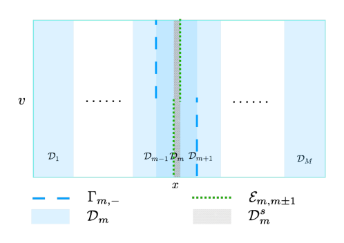
One can see that the restriction on Γm,+ssubscriptsuperscriptΓs𝑚\Gamma^{\text{s}}_{m,+} of the local solution in the domain 𝒟msubscript𝒟𝑚\mathscr{D}_{m}, would partially provide the inflow boundary condition for its neighboring domain 𝒟m±1subscript𝒟plus-or-minus𝑚1\mathscr{D}_{m\pm 1}. This fact will be used later to update local solutions in each iteration of Schwarz method. Figure 3 illustrates our setup.
Refer to caption
Fig. 3: An overlapping domain decomposition of 𝒟𝒟\mathscr{D}. The horizontal direction and vertical direction represent 𝒦𝒦\mathcal{K} and 𝒱𝒱\mathcal{V}, respectively. For simplicity, we consider only the case in which both 𝒦𝒦\mathcal{K} and 𝒱𝒱\mathcal{V} are subsets of the real line. Each subdomain 𝒟msubscript𝒟𝑚\mathscr{D}_{m} overlaps the neighboring two subdomains 𝒟m1subscript𝒟𝑚1\mathscr{D}_{m-1} and 𝒟m+1subscript𝒟𝑚1\mathscr{D}_{m+1} (except that 𝒟1subscript𝒟1\mathscr{D}_{1} and 𝒟Msubscript𝒟𝑀\mathscr{D}_{M} have one neighboring subdomain). The inflow boundary for 𝒟msubscript𝒟𝑚\mathscr{D}_{m}, Γm,subscriptΓ𝑚\Gamma_{m,-}, and the inflow boundary for 𝒟m±1subscript𝒟plus-or-minus𝑚1\mathscr{D}_{m\pm 1} confined in 𝒟msubscript𝒟𝑚\mathscr{D}_{m}, which is denoted by m,m±1subscript𝑚plus-or-minus𝑚1\mathcal{E}_{m,m\pm 1}, is also illustrated.

The Schwarz method is an iterative algorithm that updates solutions confined to different subdomains by exchanging information between iterations. In this setting, we update the values on m,m±1subscript𝑚plus-or-minus𝑚1\mathcal{E}_{m,m\pm 1} using the newly computed solutions in each subdomain, repeating the process until the solution converges. To be more specific, we denote by ϕmksubscriptsuperscriptitalic-ϕ𝑘𝑚\phi^{k}_{m} the restriction of the solution at the k𝑘kth step of the Schwarz process on patch m𝑚m, confined to the partial boundary Γm,subscriptΓ𝑚\Gamma_{m,-}, that is,

ϕmk:=uk|Γm,ϕk:={ϕ1k,,ϕMk}.formulae-sequenceassignsubscriptsuperscriptitalic-ϕ𝑘𝑚evaluated-atsuperscript𝑢𝑘subscriptΓ𝑚assignsuperscriptitalic-ϕ𝑘subscriptsuperscriptitalic-ϕ𝑘1subscriptsuperscriptitalic-ϕ𝑘𝑀\phi^{k}_{m}:=u^{k}|_{\Gamma_{m,-}}\,\quad\phi^{k}:=\{\phi^{k}_{1},\dotsc,\phi^{k}_{M}\}.

The k𝑘kth iteration of the Schwarz method can be expressed as a mapping from the ϕksuperscriptitalic-ϕ𝑘\phi^{k} to ϕk+1superscriptitalic-ϕ𝑘1\phi^{k+1}, obtained by exchanging the boundary conditions between adjacent patches and solving the RTE. We denote this mapping by 𝒫𝒫\mathcal{P}, as follows:

ϕk+1=𝒫(ϕk).superscriptitalic-ϕ𝑘1𝒫superscriptitalic-ϕ𝑘\phi^{k+1}=\mathcal{P}(\phi^{k}).

We terminate at an iteration k𝑘k for which the difference between ϕksuperscriptitalic-ϕ𝑘\phi^{k} and ϕk+1superscriptitalic-ϕ𝑘1\phi^{k+1} falls below a given tolerance.

The evaluation of map 𝒫𝒫\mathcal{P} amounts to evaluation and assembly of the individual maps 𝒫m(ϕm)subscript𝒫𝑚subscriptitalic-ϕ𝑚\mathcal{P}_{m}(\phi_{m}), m=1,2,,M𝑚12𝑀m=1,2,\dotsc,M, and is defined by the following procedure.

  • step 1

    Define the following solution map

    𝒮m:L2(Γm,;|nv|)HA(𝒟m)ϕu.:subscript𝒮𝑚absentsuperscript𝐿2subscriptΓ𝑚𝑛𝑣subscript𝐻𝐴subscript𝒟𝑚missing-subexpressionitalic-ϕmaps-to𝑢\begin{aligned} \mathcal{S}_{m}:\quad&L^{2}(\Gamma_{m,-};|n\cdot v|)&\rightarrow\quad&H_{A}(\mathscr{D}_{m})\\ &\phi&\mapsto\quad&u\end{aligned}\,. (12)

    by solving RTE on domain 𝒟msubscript𝒟𝑚\mathscr{D}_{m}:

    {vxu(x,v)=1εσδ(x)u(x,v)in𝒟mu(x,v)=ϕ(x,v)onΓm,,cases𝑣subscript𝑥𝑢𝑥𝑣1𝜀superscript𝜎𝛿𝑥𝑢𝑥𝑣insubscript𝒟𝑚𝑢𝑥𝑣italic-ϕ𝑥𝑣onsubscriptΓ𝑚\begin{cases}v\cdot\nabla_{x}u(x,v)=\frac{1}{\varepsilon}\sigma^{\delta}(x)\mathcal{L}u(x,v)&\quad\text{in}\quad\mathscr{D}_{m}\\ u(x,v)=\phi(x,v)&\quad\text{on}\quad\Gamma_{m,-}\end{cases}\,, (13)

    Obtain the solution um=𝒮m(ϕm)subscript𝑢𝑚subscript𝒮𝑚subscriptitalic-ϕ𝑚u_{m}=\mathcal{S}_{m}(\phi_{m}) in each subdomain 𝒟msubscript𝒟𝑚\mathscr{D}_{m} with boundary conditions ϕmsubscriptitalic-ϕ𝑚\phi_{m}. Here HA(𝒟m)subscript𝐻𝐴subscript𝒟𝑚H_{A}(\mathscr{D}_{m}) is a functional space where the trace of u𝑢u over the boundary Γm,±subscriptΓ𝑚plus-or-minus\Gamma_{m,\pm} is well defined (see the Appendix for details).

  • step 2

    Confine the solution umsubscript𝑢𝑚u_{m} on the boundaries:

    ϕm1+=umonm,m1andϕm+1+=umonm,m+1,formulae-sequencesuperscriptsubscriptitalic-ϕ𝑚1subscript𝑢𝑚onsubscript𝑚𝑚1andsuperscriptsubscriptitalic-ϕ𝑚1subscript𝑢𝑚onsubscript𝑚𝑚1\displaystyle\phi_{m-1}^{+}=u_{m}\quad\text{on}\;\mathcal{E}_{m,m-1}\quad\text{and}\quad\phi_{m+1}^{+}=u_{m}\quad\text{on}\;\mathcal{E}_{m,m+1}\,, (14)

    where ϕm1+subscriptsuperscriptitalic-ϕ𝑚1\phi^{+}_{m-1} and ϕm+1+subscriptsuperscriptitalic-ϕ𝑚1\phi^{+}_{m+1} are the boundary values transmitted to the next iteration of the Schwarz procedure.

𝒫msubscript𝒫𝑚\mathcal{P}_{m} is the boundary-to-boundary map that maps the boundary condition on Γm,subscriptΓ𝑚\Gamma_{m,-} to the boundary values on the adjacent subdomains (Γm,+s=m,m+1m,m1superscriptsubscriptΓ𝑚𝑠subscript𝑚𝑚1subscript𝑚𝑚1\Gamma_{m,+}^{s}=\mathcal{E}_{m,m+1}\cup\mathcal{E}_{m,m-1}):

𝒫m:L2(Γm,;|nv|)L2(Γm,+s;|nv|)ϕu|Γm,+s.:subscript𝒫𝑚absentsuperscript𝐿2subscriptΓ𝑚𝑛𝑣superscript𝐿2subscriptsuperscriptΓs𝑚𝑛𝑣missing-subexpressionitalic-ϕmaps-toevaluated-at𝑢superscriptsubscriptΓ𝑚𝑠\begin{aligned} \mathcal{P}_{m}:\quad&L^{2}(\Gamma_{m,-};|n\cdot v|)&\rightarrow\quad&L^{2}(\Gamma^{\text{s}}_{m,+};|n\cdot v|)\\ &\phi&\mapsto\quad&u|_{\Gamma_{m,+}^{s}}\end{aligned}\,. (15)

This map 𝒫msubscript𝒫𝑚\mathcal{P}_{m} is a well-defined operator, as we show in Theorem 36. It can be regarded as a composition of 𝒮msubscript𝒮𝑚\mathcal{S}_{m} and a trace operator, as follows:

𝒫m:ϕm𝒮mumum|Γm,+s.:subscript𝒫𝑚subscript𝒮𝑚subscriptitalic-ϕ𝑚subscript𝑢𝑚evaluated-atsubscript𝑢𝑚subscriptsuperscriptΓs𝑚\mathcal{P}_{m}:\;\phi_{m}\xrightarrow{\mathcal{S}_{m}}u_{m}\rightarrow u_{m}|_{\Gamma^{\text{s}}_{m,+}}\,. (16)

Note that um|Γm,+sevaluated-atsubscript𝑢𝑚subscriptsuperscriptΓs𝑚u_{m}|_{\Gamma^{\text{s}}_{m,+}} provides the boundary condition for the adjacent subdomains ϕm±1subscriptitalic-ϕplus-or-minus𝑚1\phi_{m\pm 1} in the next Schwarz iteration, seen as in equation (14). The full map 𝒫𝒫\mathcal{P} is obtained by collecting the action of 𝒫msubscript𝒫𝑚\mathcal{P}_{m} for all subdomains m=1,2,,M𝑚12𝑀m=1,2,\dotsc,M.

As initial conditions for the Schwarz process, we set

ϕm,0=0,m=1,2,,M,formulae-sequencesuperscriptsubscriptitalic-ϕ𝑚00𝑚12𝑀\phi_{m,-}^{0}=0\,,\quad m=1,2,\dotsc,M, (17)

except at the physical boundary, where we impose given boundary conditions:

ϕ1,0=ϕbdryonΓΓ1,,andϕM,0=ϕbdryonΓΓM,.formulae-sequencesuperscriptsubscriptitalic-ϕ10superscriptitalic-ϕbdryonsubscriptΓsubscriptΓ1andsuperscriptsubscriptitalic-ϕ𝑀0superscriptitalic-ϕbdryonsubscriptΓsubscriptΓ𝑀\displaystyle\phi_{1,-}^{0}=\phi^{\text{bdry}}\quad\text{on}\quad\Gamma_{-}\cap\Gamma_{1,-}\,,\quad\text{and}\quad\phi_{M,-}^{0}=\phi^{\text{bdry}}\quad\text{on}\quad\Gamma_{-}\cap\Gamma_{M,-}\,. (18)

When convergence to a given tolerance is achieved, the latest solutions may not perfectly match at the overlapping areas. To assemble the global solution, we define a suitable set of partition-of-unity functions {ηm(x)}subscript𝜂𝑚𝑥\{\eta_{m}(x)\} for the subdomains 𝒦msubscript𝒦𝑚\mathcal{K}_{m}, whose properties are as follows:

0<ηm(x)1,ηm(x)formulae-sequence0subscript𝜂𝑚𝑥1subscript𝜂𝑚𝑥\displaystyle 0<\eta_{m}(x)\leq 1,\;\;\eta_{m}(x) =0for x𝒦m and all m=1,2,,M;absent0for x𝒦m and all m=1,2,,M\displaystyle=0\;\;\mbox{for $x\notin\mathcal{K}_{m}$ and all $m=1,2,\dotsc,M$};
m=1Mηm(x)superscriptsubscript𝑚1𝑀subscript𝜂𝑚𝑥\displaystyle\sum_{m=1}^{M}\eta_{m}(x) 1,for all x𝒦.absent1for all x𝒦.\displaystyle\equiv 1\,,\quad\mbox{for all $x\in\mathcal{K}$.}

We construct the global solution by setting

ufinal(x,v)=m=1Mum(x,v)ηm(x).superscript𝑢final𝑥𝑣superscriptsubscript𝑚1𝑀subscript𝑢𝑚𝑥𝑣subscript𝜂𝑚𝑥u^{\text{final}}(x,v)=\sum_{m=1}^{M}u_{m}(x,v)\eta_{m}(x)\,. (19)

The method is summarized in Algorithm 3.

Algorithm 3 Schwarz Method for RTE
1:Input: global boundary conditions ϕbdrysuperscriptitalic-ϕbdry\phi^{\text{bdry}} and error tolerance τ𝜏\tau;
2:Set t0𝑡0t\leftarrow 0; Initialize ϕm0superscriptsubscriptitalic-ϕ𝑚0\phi_{m}^{0} from boundary conditions (17) and (18);
3:Repeat
4:     tt+1𝑡𝑡1t\leftarrow t+1;
5:     For m=1,,M𝑚1𝑀m=1,\ldots,M      
6:         umt𝒮m(ϕmt1)subscriptsuperscript𝑢𝑡𝑚subscript𝒮𝑚superscriptsubscriptitalic-ϕ𝑚𝑡1u^{t}_{m}\leftarrow\mathcal{S}_{m}(\phi_{m}^{t-1}) via (13);
7:         ϕm±1tumt|m,m±1superscriptsubscriptitalic-ϕplus-or-minus𝑚1𝑡evaluated-atsuperscriptsubscript𝑢𝑚𝑡subscript𝑚plus-or-minus𝑚1\phi_{m\pm 1}^{t}\leftarrow u_{m}^{t}|_{\mathcal{E}_{m,m\pm 1}} via trace restrictions (14);      
8:     EndFor
9:     errormϕmtϕmt1errorsubscript𝑚normsuperscriptsubscriptitalic-ϕ𝑚𝑡superscriptsubscriptitalic-ϕ𝑚𝑡1\text{error}\leftarrow\sum_{m}\|\phi_{m}^{t}-\phi_{m}^{t-1}\|;
10:Until errorτerror𝜏\text{error}\leq\tau;
11:Assemble the final solution using (19);
12:Return: final solution ufinalsuperscript𝑢finalu^{\text{final}}.

The Schwarz approach has several advantages. First, it is easy to implement in parallel, since the main computations (13) and (14) can be solved simultaneously for the subdomains m=1,2,,M𝑚12𝑀m=1,2,\dotsc,M. In fact, one could even use different solvers in different subdomains, when appropriate (for example, when there is prior information about inhomogeneity of the medium). Second, computing solutions in each subdomain is significantly cheaper than for the full domain. It saves storage cost and computation time, especially when stoge and computation scale superlinearly with the size of the domain.

The disadvantage of the Schwarz approach is that it requires multiple iterations for convergence. Since 𝒫msubscript𝒫𝑚\mathcal{P}_{m} needs to be reevaluated at each iteration for each subdomain 𝒟msubscript𝒟𝑚\mathscr{D}_{m}, and it calls for the computation of 𝒮msubscript𝒮𝑚\mathcal{S}_{m}, finding the local solutions with the given boundary condition quickly is the key to the success of the entire algorithm. In the following sections, we identify the operator that can be efficiently compressed, aiming at improving the efficiency of evaluating 𝒫msubscript𝒫𝑚\mathcal{P}_{m}, or 𝒮msubscript𝒮𝑚\mathcal{S}_{m}.

3.2 Identifying the Operator to be Compressed

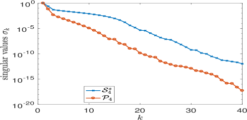
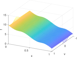
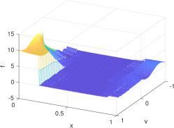
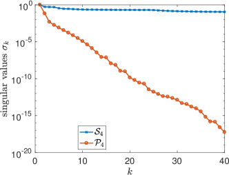
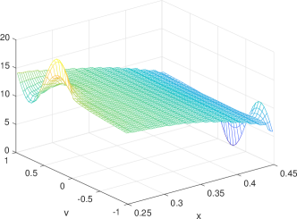
As discussed in Section 2.3, one should be able to reveal and exploit the low-rankness in homogenizable equations. In our setting, the local equation (13) has a homogenization limit when ε𝜀\varepsilon and δ𝛿\delta are small, so we expect the map from boundary conditions to local interior solutions (upon eliminating a boundary layer) to be of low rank. Indeed, we see this phenomenon in Figure 4, where we plot all normalized singular values of the discrete representation of 𝒮4subscript𝒮4\mathcal{S}_{4} and 𝒫4subscript𝒫4\mathcal{P}_{4}. A solution with an inhomogeneous boundary condition can have strong boundary layer effect. These boundary layer effects are included in 𝒮msubscript𝒮𝑚\mathcal{S}_{m}, an operator that maps the boundary condition to the solution in the entire region (including the boundary layer), destroying the desired low-rank structure. However, the operator 𝒫msubscript𝒫𝑚\mathcal{P}_{m} looks only at the solution confined to a small interior set ΓmssubscriptsuperscriptΓs𝑚\Gamma^{\text{s}}_{m}, and has a much faster decay in its singular values. This observation resonates with the argument in Remark 2: the homogenization limit concerns mainly the behavior of the solution in the interior of the (sub)domain, while the behavior of the solution in boundary layers is usually still far from “equilibrium”.
Refer to caption
Refer to caption
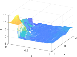
Fig. 4: Left: Singular values of 𝒮4subscript𝒮4\mathcal{S}_{4} and 𝒫4subscript𝒫4\mathcal{P}_{4}. Right: A solution with inhomogeneous boundary condition, exhibiting the boundary layer effect. (ε,δ)=(1/81,1/81)𝜀𝛿181181(\varepsilon,\delta)=(1/81,1/81) in both cases. The domain is chosen to be (x,v)[3/20,7/20]×[1,1]𝑥𝑣32072011(x,v)\in[3/20,7/20]\times[-1,1] with discretization parameters Δx=0.002Δ𝑥0.002\Delta x=0.002 and Δv=0.05Δ𝑣0.05\Delta v=0.05. In x𝑥x direction we apply upwind and in v𝑣v direction we apply the classical Snsubscript𝑆𝑛S_{n} (discrete ordinates) method. The resulting algebra problem is computed using GMRES [34].

Thus 𝒫msubscript𝒫𝑚\mathcal{P}_{m} is a more suitable object for compression, so we seek a fast solver to approximate 𝒫m(ϕm)subscript𝒫𝑚subscriptitalic-ϕ𝑚\mathcal{P}_{m}(\phi_{m}) for any input ϕmsubscriptitalic-ϕ𝑚\phi_{m}, by making use of Randomized SVD (Algorithm 2). This method requires us to apply the operator 𝒫msubscript𝒫𝑚\mathcal{P}_{m} to random inputs, which amounts to finding the local solution in 𝒟msubscript𝒟𝑚\mathscr{D}_{m} with randomly constructed boundary conditions, and then confining it to Γm,+ssubscriptsuperscriptΓs𝑚\Gamma^{\text{s}}_{m,+}. Following (16), the evaluation f=𝒫m(r)𝑓subscript𝒫𝑚𝑟f=\mathcal{P}_{m}(r) is defined as

f=u|Γm,+swhere u solves{vxu(x,v)=1εσδ(x)u(x,v)in𝒟mu(x,v)=r(x,v)onΓm,.𝑓evaluated-at𝑢subscriptsuperscriptΓs𝑚where u solvescases𝑣subscript𝑥𝑢𝑥𝑣1𝜀superscript𝜎𝛿𝑥𝑢𝑥𝑣insubscript𝒟𝑚𝑢𝑥𝑣𝑟𝑥𝑣onsubscriptΓ𝑚f=u|_{\Gamma^{\text{s}}_{m,+}}\quad\text{where $u$ solves}\quad\begin{cases}v\cdot\nabla_{x}u(x,v)=\frac{1}{\varepsilon}\sigma^{\delta}(x)\mathcal{L}u(x,v)&\quad\text{in}\quad\mathscr{D}_{m}\\ u(x,v)=r(x,v)&\quad\text{on}\quad\Gamma_{m,-}\end{cases}\,.

Finding 𝒫msubscriptsuperscript𝒫𝑚\mathcal{P}^{\ast}_{m}, the adjoint of 𝒫msubscript𝒫𝑚\mathcal{P}_{m}, is much more complicated, as we show in the following theorem, whose proof appears in the Appendix.

Theorem 6.

The adjoint operator 𝒫msubscriptsuperscript𝒫𝑚\mathcal{P}^{\ast}_{m} is defined by

𝒫m:L2(Γm,+s;|nv|)L2(Γm,;|nv|)ψh|Γm,,:subscriptsuperscript𝒫𝑚absentsuperscript𝐿2subscriptsuperscriptΓ𝑠𝑚𝑛𝑣superscript𝐿2subscriptΓ𝑚𝑛𝑣missing-subexpression𝜓maps-toevaluated-atsubscriptΓ𝑚\begin{aligned} \mathcal{P}^{\ast}_{m}:\quad&L^{2}(\Gamma^{s}_{m,+};|n\cdot v|)&\rightarrow\quad&L^{2}(\Gamma_{m,-};|n\cdot v|)\\ &\psi&\mapsto\quad&h|_{\Gamma_{m,-}}\end{aligned}, (20)

where hh, supported on 𝒟m\𝒟ms\subscript𝒟𝑚superscriptsubscript𝒟𝑚𝑠\mathscr{D}_{m}\backslash\mathscr{D}_{m}^{s}, satisfies:

{(vxσδε)h=0in𝒟m\𝒟msh=gonΓm,sh=0onΓm,+,cases𝑣subscript𝑥superscript𝜎𝛿𝜀0in\subscript𝒟𝑚superscriptsubscript𝒟𝑚𝑠𝑔onsuperscriptsubscriptΓ𝑚𝑠0onsubscriptΓ𝑚\begin{cases}(-v\cdot\nabla_{x}-\frac{\sigma^{\delta}}{\varepsilon}\mathcal{L})h=0\quad&\text{in}\quad\mathscr{D}_{m}\backslash\mathscr{D}_{m}^{s}\\ h=g\quad&\text{on}\quad\Gamma_{m,-}^{s}\\ h=0\quad&\text{on}\quad\Gamma_{m,+}\\ \end{cases}\,, (21)

in which g𝑔g is the solution to:

{(vxσε)g=0in𝒟msg=ψ+h|Γm,+sonΓm,+s.cases𝑣subscript𝑥𝜎𝜀𝑔0insuperscriptsubscript𝒟𝑚𝑠𝑔𝜓evaluated-atsubscriptsuperscriptΓ𝑠𝑚onsuperscriptsubscriptΓ𝑚𝑠\begin{cases}(-v\cdot\nabla_{x}-\frac{\sigma}{\varepsilon}\mathcal{L})g=0\quad&\text{in}\quad\mathscr{D}_{m}^{s}\\ g=\psi+h|_{\Gamma^{s}_{m,+}}\quad&\text{on}\quad\Gamma_{m,+}^{s}\end{cases}\,. (22)

The operators 𝒫msubscriptsuperscript𝒫𝑚\mathcal{P}^{\ast}_{m} and 𝒫msubscript𝒫𝑚\mathcal{P}_{m} are adjoint in the sense that:

𝒫mϕ,ψΓm,s=ϕ,𝒫mψΓm,+s,subscriptsubscript𝒫𝑚italic-ϕ𝜓superscriptsubscriptΓ𝑚𝑠subscriptitalic-ϕsubscriptsuperscript𝒫𝑚𝜓subscriptsuperscriptΓ𝑠𝑚\langle\mathcal{P}_{m}\phi,\psi\rangle_{\Gamma_{m,-}^{s}}=\langle\phi,\mathcal{P}^{\ast}_{m}\psi\rangle_{\Gamma^{s}_{m,+}}\,, (23)

where ,Γm,+ssubscriptsuperscriptsubscriptΓ𝑚𝑠\langle\cdot,\cdot\rangle_{\Gamma_{m,+}^{s}} and ,Γm,subscriptsubscriptΓ𝑚\langle\cdot,\cdot\rangle_{\Gamma_{m,-}} are weighted-L2superscript𝐿2L^{2} inner products on L2(Γm,+s;|nv|)superscript𝐿2subscriptsuperscriptΓs𝑚𝑛𝑣L^{2}(\Gamma^{\text{s}}_{m,+};|n\cdot v|) and L2(Γm,;|nv|)superscript𝐿2subscriptΓ𝑚𝑛𝑣L^{2}(\Gamma_{m,-};|n\cdot v|), respectively, defined by

f,gΓm,+s=Γm,+sfg|nv|dxdv,andf,gΓm,=Γm,fg|nv|dxdv.formulae-sequencesubscript𝑓𝑔superscriptsubscriptΓ𝑚𝑠subscriptsubscriptsuperscriptΓs𝑚𝑓𝑔𝑛𝑣differential-d𝑥differential-d𝑣andsubscript𝑓𝑔subscriptΓ𝑚subscriptsubscriptΓ𝑚𝑓𝑔𝑛𝑣differential-d𝑥differential-d𝑣\langle f\,,g\rangle_{\Gamma_{m,+}^{s}}=\int_{\Gamma^{\text{s}}_{m,+}}fg|n\cdot v|\,\mathrm{d}{x}\,\mathrm{d}{v}\,,\quad\text{and}\quad\langle f\,,g\rangle_{\Gamma_{m,-}}=\int_{\Gamma_{m,-}}fg|n\cdot v|\,\mathrm{d}{x}\,\mathrm{d}{v}\,.

The computation involved in finding the adjoint operator is complicated. It requires the computation of two adjoint RTEs over 𝒟mssuperscriptsubscript𝒟𝑚s\mathscr{D}_{m}^{\text{s}} and 𝒟m\𝒟ms\subscript𝒟𝑚superscriptsubscript𝒟𝑚s\mathscr{D}_{m}\backslash\mathscr{D}_{m}^{\text{s}}, respectively, that are coupled in a nontrivial fashion through the boundary conditions, as seen in (21) and (22). We further note that the measure is not the standard Lebesgue measure, but rather is weighted by |nv|𝑛𝑣|n\cdot v|.

3.3 Design of the Adjoint Map for 𝒮mssubscriptsuperscript𝒮s𝑚\mathcal{S}^{\text{s}}_{m}

Although the operator 𝒫msubscript𝒫𝑚\mathcal{P}_{m} is of approximate low-rank, its adjoint 𝒫msuperscriptsubscript𝒫𝑚\mathcal{P}_{m}^{\ast}, which is needed to compute the low-rank approximation, is complicated. The operator 𝒮msubscript𝒮𝑚\mathcal{S}_{m}, on the other hand, is not compressible, but its adjoint is relatively easy to find. In this section, we show that we can approximate 𝒫msubscript𝒫𝑚\mathcal{P}_{m} by an approximately low-rank operator based on 𝒮msubscript𝒮𝑚\mathcal{S}_{m} whose adjoint is easy to find.

Since 𝒮msubscript𝒮𝑚\mathcal{S}_{m} has slow singular decay mainly because it contains too much information from the boundary layer, we consider a restriction of this operator from 𝒟msubscript𝒟𝑚\mathscr{D}_{m} to 𝒟mssuperscriptsubscript𝒟𝑚s\mathscr{D}_{m}^{\text{s}}, which we call 𝒮mssubscriptsuperscript𝒮s𝑚\mathcal{S}^{\text{s}}_{m}. The restriction to 𝒟mssuperscriptsubscript𝒟𝑚s\mathscr{D}_{m}^{\text{s}} eliminates most of the effects of the boundary layer. This operator is defined as follows.

𝒮ms:L2(Γm,;|nv|)L2(𝒟ms)ϕus,:subscriptsuperscript𝒮s𝑚absentsuperscript𝐿2subscriptΓ𝑚𝑛𝑣superscript𝐿2subscriptsuperscript𝒟s𝑚missing-subexpressionitalic-ϕmaps-tosuperscript𝑢s\begin{aligned} \mathcal{S}^{\text{s}}_{m}:\quad&L^{2}(\Gamma_{m,-};|n\cdot v|)&\rightarrow\quad&L^{2}(\mathscr{D}^{\text{s}}_{m})\\ &\phi&\mapsto\quad&u^{\text{s}}\end{aligned}\,, (24)

where ums=um|𝒟mssuperscriptsubscript𝑢𝑚sevaluated-atsubscript𝑢𝑚subscriptsuperscript𝒟s𝑚u_{m}^{\text{s}}=u_{m}|_{\mathscr{D}^{\text{s}}_{m}} and um=𝒮mϕsubscript𝑢𝑚subscript𝒮𝑚italic-ϕu_{m}=\mathcal{S}_{m}\phi. The advantages of using this operator are threefold.

  • 1.

    𝒫msubscript𝒫𝑚\mathcal{P}_{m} can be defined easily in terms of 𝒮mssubscriptsuperscript𝒮s𝑚\mathcal{S}^{\text{s}}_{m}. Nothing is lost by comparison with (16); we have

    𝒫m:ϕm𝒮msumsums|Γm,+s,:subscript𝒫𝑚subscriptsuperscript𝒮s𝑚subscriptitalic-ϕ𝑚superscriptsubscript𝑢𝑚sevaluated-atsubscriptsuperscript𝑢s𝑚subscriptsuperscriptΓs𝑚\mathcal{P}_{m}:\;\phi_{m}\xrightarrow{\mathcal{S}^{\text{s}}_{m}}u_{m}^{\text{s}}\rightarrow u^{\text{s}}_{m}|_{\Gamma^{\text{s}}_{m,+}}\,, (25)

    and ums|Γm,+sevaluated-atsubscriptsuperscript𝑢s𝑚subscriptsuperscriptΓs𝑚u^{\text{s}}_{m}|_{\Gamma^{\text{s}}_{m,+}} once again serves as the new boundary condition ϕm±1subscriptitalic-ϕplus-or-minus𝑚1\phi_{m\pm 1}, as in equation (14). Note that the trace in (25) is well defined, as 𝒮msubscript𝒮𝑚\mathcal{S}_{m} maps boundary conditions to HA(𝒟m)subscript𝐻𝐴subscript𝒟𝑚H_{A}(\mathscr{D}_{m}), so the image of its restriction to 𝒟mssuperscriptsubscript𝒟𝑚s\mathscr{D}_{m}^{\text{s}} has a trace on the boundary Γm,+ssuperscriptsubscriptΓ𝑚s\Gamma_{m,+}^{\text{s}} of 𝒟mssuperscriptsubscript𝒟𝑚s\mathscr{D}_{m}^{\text{s}}.

  • 2.

    Because effects from boundary layers are excluded in 𝒮mssuperscriptsubscript𝒮𝑚s\mathcal{S}_{m}^{\text{s}}, it can be expected to have approximate low rank. Figure 5 shows that the decay rate of 𝒮mssubscriptsuperscript𝒮s𝑚\mathcal{S}^{\text{s}}_{m} (upon discretization) is almost the same as for 𝒫msubscript𝒫𝑚\mathcal{P}_{m}.

    Refer to caption
    Fig. 5: Singular values of 𝒮4ssuperscriptsubscript𝒮4𝑠\mathcal{S}_{4}^{s} and 𝒫4subscript𝒫4\mathcal{P}_{4} when (ε,δ)=(1/81,1/81)𝜀𝛿181181(\varepsilon,\delta)=(1/81,1/81).
  • 3.

    The adjoint is easy to compute, as we show next, in Theorem 7.

Theorem 7.

The adjoint of 𝒮mssuperscriptsubscript𝒮𝑚s\mathcal{S}_{m}^{\text{s}} is defined as follows:

(𝒮ms):L2(𝒟ms)L2(Γm,;|nv|)gh|Γm,,:superscriptsuperscriptsubscript𝒮𝑚sabsentsuperscript𝐿2subscriptsuperscript𝒟s𝑚superscript𝐿2subscriptΓ𝑚𝑛𝑣missing-subexpression𝑔maps-toevaluated-atsubscriptΓ𝑚\begin{aligned} \left(\mathcal{S}_{m}^{\text{s}}\right)^{\ast}:\ &L^{2}(\mathscr{D}^{\text{s}}_{m})\ &\rightarrow\ &L^{2}(\Gamma_{m,-};|n\cdot v|)\\ &g\ &\mapsto\ &h|_{\Gamma_{m,-}}\end{aligned}, (26)

where hh solves the adjoint RTE over 𝒟msubscript𝒟𝑚\mathscr{D}_{m}, which is

{(vx1εσδ(x))h=g~in𝒟mh=0onΓm,+,cases𝑣subscript𝑥1𝜀superscript𝜎𝛿𝑥~𝑔insubscript𝒟𝑚0onsubscriptΓ𝑚\begin{cases}(-v\cdot\nabla_{x}-\frac{1}{\varepsilon}\sigma^{\delta}(x)\mathcal{L})h=\tilde{g}\quad&\text{in}\quad\mathscr{D}_{m}\\ h=0\ \quad&\text{on}\quad\Gamma_{m,+}\end{cases}\,, (27)

and the source g~~𝑔\tilde{g} is the trivial extension of g𝑔g over 𝒟msubscript𝒟𝑚\mathscr{D}_{m}, that is,

g~=gfor (x,v)𝒟msandg~=0for (x,v)𝒟m\𝒟ms.formulae-sequence~𝑔𝑔for (x,v)𝒟msand~𝑔0for (x,v)𝒟m\𝒟ms\tilde{g}=g\,\;\;\mbox{for $(x,v)\in\mathscr{D}^{\text{s}}_{m}$}\quad\text{and}\quad\tilde{g}=0\;\;\mbox{for $(x,v)\in\mathscr{D}_{m}\backslash\mathscr{D}_{m}^{\text{s}}$}.
Proof.

We need to show that

g,𝒮msϕ𝒟ms=(𝒮ms)g,ϕΓm,subscript𝑔subscriptsuperscript𝒮s𝑚italic-ϕsuperscriptsubscript𝒟𝑚ssubscriptsuperscriptsuperscriptsubscript𝒮𝑚s𝑔italic-ϕsubscriptΓ𝑚\langle g,\mathcal{S}^{\text{s}}_{m}\phi\rangle_{\mathscr{D}_{m}^{\text{s}}}=\langle\left(\mathcal{S}_{m}^{\text{s}}\right)^{\ast}g\,,\phi\rangle_{\Gamma_{m,-}}

for all g𝑔g and ϕitalic-ϕ\phi. Denoting by u𝑢u the solution to (13) with boundary condition ϕitalic-ϕ\phi, then the definition of 𝒮mssubscriptsuperscript𝒮s𝑚\mathcal{S}^{\text{s}}_{m} implies that the left hand side of this expression is

g,𝒮msϕ𝒟ms=𝒟msgudxdv=𝒟mg~udxdv.subscript𝑔subscriptsuperscript𝒮s𝑚italic-ϕsuperscriptsubscript𝒟𝑚ssubscriptsubscriptsuperscript𝒟s𝑚𝑔𝑢differential-d𝑥differential-d𝑣subscriptsubscript𝒟𝑚~𝑔𝑢differential-d𝑥differential-d𝑣\langle g,\mathcal{S}^{\text{s}}_{m}\phi\rangle_{\mathscr{D}_{m}^{\text{s}}}=\int_{\mathscr{D}^{\text{s}}_{m}}gu\ \,\mathrm{d}x\,\mathrm{d}v=\int_{\mathscr{D}_{m}}\tilde{g}u\,\mathrm{d}x\,\mathrm{d}v\,.

Denoting by hh the solution to (27) with source term g𝑔g, we have

𝒟mg~udxdvsubscriptsubscript𝒟𝑚~𝑔𝑢differential-d𝑥differential-d𝑣\displaystyle\int_{\mathscr{D}_{m}}\tilde{g}u\ \,\mathrm{d}x\,\mathrm{d}v =𝒟mu(vx1εσδ)hdxdvabsentsubscriptsubscript𝒟𝑚𝑢𝑣subscript𝑥1𝜀superscript𝜎𝛿differential-d𝑥differential-d𝑣\displaystyle=\int_{\mathscr{D}_{m}}u(-v\cdot\nabla_{x}-\frac{1}{\varepsilon}\sigma^{\delta}\mathcal{L})h\ \,\mathrm{d}x\,\mathrm{d}v
=Γm,uhvndxdvΓm,+uhvndxdvabsentsubscriptsubscriptΓ𝑚𝑢𝑣𝑛differential-d𝑥differential-d𝑣subscriptsubscriptΓ𝑚𝑢𝑣𝑛differential-d𝑥differential-d𝑣\displaystyle=-\int_{\Gamma_{m,-}}uhv\cdot n\,\mathrm{d}{x}\,\mathrm{d}{v}-\int_{\Gamma_{m,+}}uhv\cdot n\,\mathrm{d}{x}\,\mathrm{d}{v}
+𝒟mh(vx1εσδ)udxdvsubscriptsubscript𝒟𝑚𝑣subscript𝑥1𝜀superscript𝜎𝛿𝑢differential-d𝑥differential-d𝑣\displaystyle\qquad\qquad+\int_{\mathscr{D}_{m}}h(v\cdot\nabla_{x}-\frac{1}{\varepsilon}\sigma^{\delta}\mathcal{L})u\,\mathrm{d}{x}\,\mathrm{d}{v}
=Γm,uh|vn|dxdvabsentsubscriptsubscriptΓ𝑚𝑢𝑣𝑛differential-d𝑥differential-d𝑣\displaystyle=\int_{\Gamma_{m,-}}uh|v\cdot n|\,\mathrm{d}{x}\,\mathrm{d}{v}
=(𝒮ms)g,ϕΓm,,absentsubscriptsuperscriptsuperscriptsubscript𝒮𝑚s𝑔italic-ϕsubscriptΓ𝑚\displaystyle=\langle\left(\mathcal{S}_{m}^{\text{s}}\right)^{\ast}g,\phi\rangle_{\Gamma_{m,-}}\,,

yielding the desired result. ∎

By comparing Theorem 6 with Theorem 7, we see immediately that computing the adjoint operator (𝒮ms)superscriptsuperscriptsubscript𝒮𝑚s\left(\mathcal{S}_{m}^{\text{s}}\right)^{\ast} is significantly easier than computing 𝒫msubscriptsuperscript𝒫𝑚\mathcal{P}^{\ast}_{m}.

3.4 Low-Rank Schwarz Iteration Method

We can use (𝒮ms)superscriptsuperscriptsubscript𝒮𝑚s\left(\mathcal{S}_{m}^{\text{s}}\right)^{\ast} to implement the RSVD method to find the low-rank approximation to the operator 𝒮mssuperscriptsubscript𝒮𝑚s\mathcal{S}_{m}^{\text{s}}. Given target rank r𝑟r, and denoting the reduced operator by 𝒮m,rssuperscriptsubscript𝒮𝑚𝑟s\mathcal{S}_{m,r}^{\text{s}}, we look for functions μisubscript𝜇𝑖\mu_{i} and νisubscript𝜈𝑖\nu_{i}, and nonnegative scalars σisubscript𝜎𝑖\sigma_{i}, such that:

𝒮m,rs=iσiμi(x1,v1)νi(x2,v2),for all (x1,v1)𝒟ms and (x2,v2)Γm,,superscriptsubscript𝒮𝑚𝑟ssubscript𝑖subscript𝜎𝑖subscript𝜇𝑖subscript𝑥1subscript𝑣1subscript𝜈𝑖subscript𝑥2subscript𝑣2for all (x1,v1)𝒟ms and (x2,v2)Γm,,\mathcal{S}_{m,r}^{\text{s}}=\sum_{i}\sigma_{i}\mu_{i}(x_{1},v_{1})\nu_{i}(x_{2},v_{2})\,,\quad\mbox{for all $(x_{1},v_{1})\in\mathscr{D}_{m}^{\text{s}}$ and $(x_{2},v_{2})\in\Gamma_{m,-}$,} (28)

where μi(x1,v1)subscript𝜇𝑖subscript𝑥1subscript𝑣1\mu_{i}(x_{1},v_{1}) and νi(x2,v2)subscript𝜈𝑖subscript𝑥2subscript𝑣2\nu_{i}(x_{2},v_{2}) are obtained in Algorithm 4.

Algorithm 4 Approximation of 𝒮mssuperscriptsubscript𝒮𝑚s\mathcal{S}_{m}^{\text{s}} via RSVD
1:Given desired rank r𝑟r and oversampling parameter p𝑝p, set k:=r+passign𝑘𝑟𝑝k:=r+p;
2:Stage I
3:     Generate k𝑘k independent Gaussian test vectors ω1,,ωksubscript𝜔1subscript𝜔𝑘\omega_{1},\ldots,\omega_{k};
4:     Prepare incoming boundary conditions wi~=𝖤wi,i=1,,kformulae-sequence~subscript𝑤𝑖𝖤subscript𝑤𝑖𝑖1𝑘\widetilde{w_{i}}=\mathsf{E}w_{i}\,,i=1,\ldots,k, where 𝖤=[e1,e2,]𝖤subscript𝑒1subscript𝑒2\mathsf{E}=[e_{1},e_{2},\dotsc] collects discrete orthonormal basis functions in L2(Γm,;|nv|)superscript𝐿2subscriptΓ𝑚𝑛𝑣L^{2}(\Gamma_{m,-};|n\cdot v|);
5:     Evaluate um,i|𝒟ms=𝒮msw~i,i=1,,kformulae-sequenceevaluated-atsubscript𝑢𝑚𝑖superscriptsubscript𝒟𝑚𝑠superscriptsubscript𝒮𝑚ssubscript~𝑤𝑖𝑖1𝑘u_{m,i}|_{\mathscr{D}_{m}^{s}}=\mathcal{S}_{m}^{\text{s}}\widetilde{w}_{i}\,,i=1,\ldots,k by solving (13) with boundary conditions w~isubscript~𝑤𝑖\widetilde{w}_{i}, then taking restrictions over 𝒟mssuperscriptsubscript𝒟𝑚𝑠\mathscr{D}_{m}^{s};
6:     Construct matrix 𝖰=[q1,,qk]𝖰subscript𝑞1subscript𝑞𝑘\mathsf{Q}=[q_{1},\ldots,q_{k}] whose columns form an orthogonal basis for span{um,1|𝒟ms,,um,k|𝒟ms}evaluated-atsubscript𝑢𝑚1superscriptsubscript𝒟𝑚𝑠evaluated-atsubscript𝑢𝑚𝑘superscriptsubscript𝒟𝑚𝑠\{u_{m,1}|_{\mathscr{D}_{m}^{s}},\ldots,u_{m,k}|_{\mathscr{D}_{m}^{s}}\};
7:Stage II
8:     Prepare sources gi=[qi0]subscript𝑔𝑖subscript𝑞𝑖0g_{i}=[q_{i}\quad 0], i=1,2,,k𝑖12𝑘i=1,2,\dotsc,k, so that gi=qisubscript𝑔𝑖subscript𝑞𝑖g_{i}=q_{i} over 𝒟mssuperscriptsubscript𝒟𝑚𝑠\mathscr{D}_{m}^{s} and gi=0subscript𝑔𝑖0g_{i}=0 over 𝒟m\𝒟ms¯\subscript𝒟𝑚¯superscriptsubscript𝒟𝑚𝑠\mathscr{D}_{m}\backslash\overline{\mathscr{D}_{m}^{s}};
9:     Evaluate bi=Ygisubscript𝑏𝑖𝑌subscript𝑔𝑖b_{i}=Yg_{i} by solving (27) with gisubscript𝑔𝑖g_{i} as source, for i=1,2,,k𝑖12𝑘i=1,2,\dotsc,k, then taking restrictions over Γm,subscriptΓ𝑚\Gamma_{m,-};
10:     Form matrix 𝖡=[b1,,bk]𝖡subscript𝑏1subscript𝑏𝑘\mathsf{B}=[b_{1},\ldots,b_{k}];
11:     Compute SVD of 𝖡=𝖬~kΣk𝖭k𝖡subscript~𝖬𝑘subscriptΣ𝑘superscriptsubscript𝖭𝑘\mathsf{B}=\widetilde{\mathsf{M}}_{k}\Sigma_{k}\mathsf{N}_{k}^{\ast}, where
𝖬~k=[μ~1,,μ~k],Σk=diag{σ1,,σk},and𝖭k=[ν1,,νk];formulae-sequencesubscript~𝖬𝑘matrixsubscript~𝜇1subscript~𝜇𝑘formulae-sequencesubscriptΣ𝑘diagsubscript𝜎1subscript𝜎𝑘andsubscript𝖭𝑘matrixsubscript𝜈1subscript𝜈𝑘\widetilde{\mathsf{M}}_{k}=\begin{bmatrix}\widetilde{\mu}_{1},\ldots,\widetilde{\mu}_{k}\end{bmatrix}\,,\quad\Sigma_{k}=\text{diag}\{\sigma_{1},\ldots,\sigma_{k}\}\,,\quad\text{and}\quad\mathsf{N}_{k}=\begin{bmatrix}\nu_{1},\ldots,\nu_{k}\end{bmatrix};
12:     Compute 𝖬k:=𝖰𝖬~kassignsubscript𝖬𝑘𝖰subscript~𝖬𝑘\mathsf{M}_{k}:=\mathsf{Q}\widetilde{\mathsf{M}}_{k} and denote 𝖬k=[μ1,,μk]subscript𝖬𝑘matrixsubscript𝜇1subscript𝜇𝑘\mathsf{M}_{k}=\begin{bmatrix}\mu_{1},\ldots,\mu_{k}\end{bmatrix};
13:Return: 𝒮m,rs=i=1rσiμi(x1,v1)νi(x2,v2)superscriptsubscript𝒮𝑚𝑟ssuperscriptsubscript𝑖1𝑟subscript𝜎𝑖subscript𝜇𝑖subscript𝑥1subscript𝑣1subscript𝜈𝑖subscript𝑥2subscript𝑣2\mathcal{S}_{m,r}^{\text{s}}=\sum_{i=1}^{r}\sigma_{i}\mu_{i}(x_{1},v_{1})\nu_{i}(x_{2},v_{2}) for (x1,v1)𝒟mssubscript𝑥1subscript𝑣1superscriptsubscript𝒟𝑚s(x_{1},v_{1})\in\mathscr{D}_{m}^{\text{s}} and (x2,v2)Γm,subscript𝑥2subscript𝑣2subscriptΓ𝑚(x_{2},v_{2})\in\Gamma_{m,-}.

We note that in this algorithm, k𝑘k and r𝑟r could be hard to choose ahead of time. Numerically we can choose it “on-the-fly”. This means we simply set an accuracy threshold and stop the process once the newly computed um,i|𝒟msevaluated-atsubscript𝑢𝑚𝑖superscriptsubscript𝒟𝑚𝑠u_{m,i}|_{\mathscr{D}_{m}^{s}} falls almost in the previous generated space within the preset error tolerance. In terms of the low-rank operator 𝒮m,rssubscriptsuperscript𝒮s𝑚𝑟\mathcal{S}^{\text{s}}_{m,r}, the procedure (25) is reduced further to

𝒫m,r:ϕm𝒮m,rsumsums|Γm,+s,:subscript𝒫𝑚𝑟subscriptsuperscript𝒮s𝑚𝑟subscriptitalic-ϕ𝑚subscriptsuperscript𝑢s𝑚evaluated-atsubscriptsuperscript𝑢s𝑚subscriptsuperscriptΓs𝑚\mathcal{P}_{m,r}:\;\phi_{m}\xrightarrow{\mathcal{S}^{\text{s}}_{m,r}}u^{\text{s}}_{m}\rightarrow u^{\text{s}}_{m}|_{\Gamma^{\text{s}}_{m,+}}\,, (29)

and we once again use ums|Γm,+sevaluated-atsubscriptsuperscript𝑢s𝑚subscriptsuperscriptΓs𝑚u^{\text{s}}_{m}|_{\Gamma^{\text{s}}_{m,+}} to obtain the solutions ϕm±1subscriptitalic-ϕplus-or-minus𝑚1\phi_{m\pm 1} to be used at the next time step, as in equation (14).

The procedure we have just outlined provides a much cheaper way to evaluate 𝒫𝒫\mathcal{P} in (16) for the following reasons.

  1. 1.

    𝒮mssuperscriptsubscript𝒮𝑚s\mathcal{S}_{m}^{\text{s}} maps the boundary condition to the interior of the subdomain, and it is cheaper to evaluate than 𝒮msubscript𝒮𝑚\mathcal{S}_{m}, whose range has a bigger support.

  2. 2.

    The format in (28) guides the evaluation of 𝒮m,rs(ϕm)superscriptsubscript𝒮𝑚𝑟ssubscriptitalic-ϕ𝑚\mathcal{S}_{m,r}^{\text{s}}(\phi_{m}); we have

    𝒮m,rs(ϕm)=i=1kσiui(x1,v1)Γm,ϕm(x2,v2)v(x2,v2)|nx2v2|dx2dv2.superscriptsubscript𝒮𝑚𝑟ssubscriptitalic-ϕ𝑚superscriptsubscript𝑖1𝑘subscript𝜎𝑖subscript𝑢𝑖subscript𝑥1subscript𝑣1subscriptsubscriptΓ𝑚subscriptitalic-ϕ𝑚subscript𝑥2subscript𝑣2𝑣subscript𝑥2subscript𝑣2subscript𝑛subscript𝑥2subscript𝑣2differential-dsubscript𝑥2differential-dsubscript𝑣2\mathcal{S}_{m,r}^{\text{s}}(\phi_{m})=\sum_{i=1}^{k}\sigma_{i}u_{i}(x_{1},v_{1})\int_{\Gamma_{m,-}}\phi_{m}(x_{2},v_{2})v(x_{2},v_{2})|n_{x_{2}}\cdot v_{2}|\,\,\mathrm{d}{x_{2}}\,\mathrm{d}{v_{2}}\,. (30)

    This evaluation requrires 𝒪(k|Γm,|)𝒪𝑘subscriptΓ𝑚\mathcal{O}(k|\Gamma_{m,-}|) operations, where |Γm,|subscriptΓ𝑚|\Gamma_{m,-}| is the cardinality (the number of grid points) in Γm,subscriptΓ𝑚\Gamma_{m,-}.

Algorithm 5 summarizes the complete approach using the reduced solution map. The method is divided into offline and online stages. The reduced operators 𝒮m,rssubscriptsuperscript𝒮s𝑚𝑟\mathcal{S}^{\text{s}}_{m,r} are found in the offline stage, then called repeatedly in the online stage, during the Schwarz iteration procedure.

Algorithm 5 Low-Rank Schwarz Method
1:Offline Stage:
2:     Call Algorithm 4 for all local reduced solution maps 𝒮m,rssuperscriptsubscript𝒮𝑚𝑟s\mathcal{S}_{m,r}^{\text{s}}, with m=1,,M𝑚1𝑀m=1\,,\dotsc,M;
3:Online Stage:
4:     Input: global boundary conditions ϕitalic-ϕ\phi in (7) and error tolerance τ𝜏\tau;
5:     Set t0𝑡0t\leftarrow 0 and initiate all inflow boundary conditions from (17) and (18);
6:     While error>τerror𝜏\text{error}>\tau      
7:         t=t+1𝑡𝑡1t=t+1;
8:         For m=1,,M𝑚1𝑀m=1,\ldots,M          
9:              ums𝒮m,rs(ϕmt1)subscriptsuperscript𝑢s𝑚superscriptsubscript𝒮𝑚𝑟ssuperscriptsubscriptitalic-ϕ𝑚𝑡1u^{\text{s}}_{m}\leftarrow\mathcal{S}_{m,r}^{\text{s}}(\phi_{m}^{t-1}) according to (30);
10:              ϕm±1t=ums|m,m±1superscriptsubscriptitalic-ϕplus-or-minus𝑚1𝑡evaluated-atsubscriptsuperscript𝑢s𝑚subscript𝑚plus-or-minus𝑚1\phi_{m\pm 1}^{t}=u^{\text{s}}_{m}|_{\mathcal{E}_{m,m\pm 1}};          
11:         EndFor
12:         error=mϕmtϕmt1errorsubscript𝑚normsuperscriptsubscriptitalic-ϕ𝑚𝑡superscriptsubscriptitalic-ϕ𝑚𝑡1\text{error}=\sum_{m}\|\phi_{m}^{t}-\phi_{m}^{t-1}\|;      
13:     EndFor
14:     For m=1,,M𝑚1𝑀m=1,\ldots,M      
15:         um𝒮m(ϕmt)subscript𝑢𝑚subscript𝒮𝑚superscriptsubscriptitalic-ϕ𝑚𝑡u_{m}\leftarrow\mathcal{S}_{m}(\phi_{m}^{t});      
16:     EndFor
17:     Assemble the final solution using (19);
18:     Return: final solution ufinalsuperscript𝑢finalu^{\text{final}}.

4 Numerical examples

In this section, we present numerical examples to validate the accuracy and efficiency of our methods. We consider boundary value problem (7) with domain 𝒟=𝒦×𝒱=(0,1)×(1,1)𝒟𝒦𝒱0111\mathscr{D}=\mathcal{K}\times\mathcal{V}=(0,1)\times(-1,1) and highly oscillatory scattering coefficient σδ(x)superscript𝜎𝛿𝑥\sigma^{\delta}(x) defined by

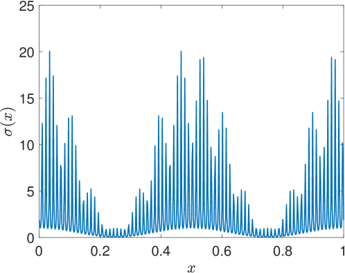
σδ(x)=1.1+cos(4πx)1.1+sin(2πx/δ)[0.047,21],superscript𝜎𝛿𝑥1.14𝜋𝑥1.12𝜋𝑥𝛿0.04721\sigma^{\delta}(x)=\frac{1.1+\cos(4\pi x)}{1.1+\sin(2\pi x/\delta)}\in[0.047,21], (31)

where δ𝛿\delta represents the period of oscillation in the spatial space. See Figure 6 for a graph of σδ(x)superscript𝜎𝛿𝑥\sigma^{\delta}(x) with δ=1/81𝛿181\delta=1/81.

Refer to caption
Fig. 6: Graph of oscillatory media with δ=1/81𝛿181\delta=1/81.

The space domain 𝒦𝒦\mathcal{K} is divided into M=10𝑀10M=10 different local subdomains 𝒦m,m=1,,Mformulae-sequencesubscript𝒦𝑚𝑚1𝑀\mathcal{K}_{m},m=1,\ldots,M, as follows:

𝒦1=(0,32M),𝒦m=(2m32M,2m+12M),m=2,,M1,𝒦M=(132M,1),formulae-sequencesubscript𝒦1032𝑀formulae-sequencesubscript𝒦𝑚2𝑚32𝑀2𝑚12𝑀formulae-sequence𝑚2𝑀1subscript𝒦𝑀132𝑀1\mathcal{K}_{1}=\left(0,\tfrac{3}{2M}\right)\,,\quad\mathcal{K}_{m}=\left(\tfrac{2m-3}{2M},\tfrac{2m+1}{2M}\right)\,,m=2,\ldots,M-1\,,\quad\mathcal{K}_{M}=\left(1-\tfrac{3}{2M},1\right),

so that each subdomain 𝒦msubscript𝒦𝑚\mathcal{K}_{m} overlaps with its neighboring subdomains 𝒦m1subscript𝒦𝑚1\mathcal{K}_{m-1} and 𝒦m+1subscript𝒦𝑚1\mathcal{K}_{m+1} (except for the subdomains 𝒦1subscript𝒦1\mathcal{K}_{1} and 𝒦Msubscript𝒦𝑀\mathcal{K}_{M} at the two ends of the domain, which overlap with just one neighbor each). The subdomains 𝒦mssuperscriptsubscript𝒦𝑚s\mathcal{K}_{m}^{\text{s}} defined in (10) are

𝒦1s=(12M,32M),𝒦ms=(m1M,mM),m=2,,M1,𝒦Ms=(132M,112M).formulae-sequencesuperscriptsubscript𝒦1s12𝑀32𝑀formulae-sequencesuperscriptsubscript𝒦𝑚s𝑚1𝑀𝑚𝑀formulae-sequence𝑚2𝑀1superscriptsubscript𝒦𝑀s132𝑀112𝑀\mathcal{K}_{1}^{\text{s}}=\left(\tfrac{1}{2M},\tfrac{3}{2M}\right)\,,\quad\mathcal{K}_{m}^{\text{s}}=\left(\tfrac{m-1}{M},\tfrac{m}{M}\right)\,,m=2,\ldots,M-1\,,\quad\mathcal{K}_{M}^{\text{s}}=\left(1-\tfrac{3}{2M},1-\tfrac{1}{2M}\right).

We thus have m,m±1={mM}×𝒱,m=1,,M1formulae-sequencesubscript𝑚plus-or-minus𝑚1𝑚𝑀𝒱𝑚1𝑀1\mathcal{E}_{m,m\pm 1}=\{\frac{m}{M}\}\times\mathcal{V}\,,\quad m=1,\ldots,M-1, while 𝒟ms:=𝒦ms×𝒱assignsuperscriptsubscript𝒟𝑚ssuperscriptsubscript𝒦𝑚s𝒱\mathscr{D}_{m}^{\text{s}}:=\mathcal{K}_{m}^{\text{s}}\times\mathcal{V} satisfies

m,m±1𝒟ms𝒟m,m=1,,M1.formulae-sequencesubscript𝑚plus-or-minus𝑚1superscriptsubscript𝒟𝑚ssubscript𝒟𝑚𝑚1𝑀1\mathcal{E}_{m,m\pm 1}\subset\mathscr{D}_{m}^{\text{s}}\subset\mathscr{D}_{m}\,,m=1,\dotsc,M-1\,.

The spatial domain 𝒦𝒦\mathcal{K} is discretized with a extreme fine mesh of size Δx=1/360Δ𝑥1360\Delta x=1/360, while the velocity domain 𝒱𝒱\mathcal{V} is discretized with a mesh of size Δv=2/40=0.05Δ𝑣2400.05\Delta v=2/40=0.05. The fine-mesh discretization is determined by δ𝛿\delta and ε𝜀\varepsilon.

4.1 Local Tests

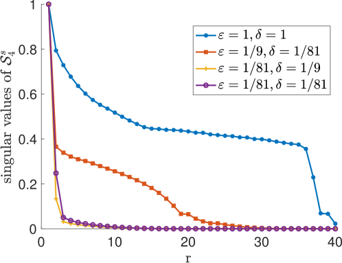
We first show that the singular values of the local solution map 𝒮mssuperscriptsubscript𝒮𝑚s\mathcal{S}_{m}^{\text{s}} indeed decay rapidly for small Knudsen number ε𝜀\varepsilon and small δ𝛿\delta. Figure 7 plots the singular values of 𝒮4ssuperscriptsubscript𝒮4s\mathcal{S}_{4}^{\text{s}} (relative to the largest singular value) for various values of (ε,δ)𝜀𝛿(\varepsilon,\delta). In the case of large values ε=δ=1𝜀𝛿1\varepsilon=\delta=1, the singular values decay slowly and low-rank structure is not present. By contrast, in the small-value regimes (ε,δ)=(1/81,1/81)𝜀𝛿181181(\varepsilon,\delta)=(1/81,1/81) and (ε,δ)=(1/81,1/9)𝜀𝛿18119(\varepsilon,\delta)=(1/81,1/9), low-rank structure is evident. As a consequence, only half or even a quarter of basis functions are needed to achieve high accuracy in approximating the local solution map 𝒮mssuperscriptsubscript𝒮𝑚s\mathcal{S}_{m}^{\text{s}}.

Refer to caption
Fig. 7: Singular value of 𝒮4ssuperscriptsubscript𝒮4s\mathcal{S}_{4}^{\text{s}}, relative to the largest singular value, plotted for various values of the parameter pair (ε,δ)𝜀𝛿(\varepsilon,\delta). The singular values decay slowly for (ε,δ)=(1,1)𝜀𝛿11(\varepsilon,\delta)=(1,1) and relatively faster for (ε,δ)=(1/9,1/81)𝜀𝛿19181(\varepsilon,\delta)=(1/9,1/81). A much faster decay is observed in other limiting regimes of (ε,δ)𝜀𝛿(\varepsilon,\delta) approaching (0,0)00(0,0).

4.2 Global Tests

We consider solving RTE (7) with scattering parameter (31) and the following inflow boundary conditions over ΓsubscriptΓ\Gamma_{-}:

ϕ(x,v)={10+sin(2πv),atx=0,v>01+sin(2πv),atx=1,v<0.italic-ϕ𝑥𝑣cases102𝜋𝑣formulae-sequenceat𝑥0𝑣012𝜋𝑣formulae-sequenceat𝑥1𝑣0\phi(x,v)=\begin{cases}10+\sin(2\pi v)\,,\;\;&\text{at}\;x=0\,,v>0\\ 1+\sin(2\pi v)\,,\;\;&\text{at}\;x=1\,,v<0.\end{cases} (32)

We approximate 𝒮mssuperscriptsubscript𝒮𝑚s\mathcal{S}_{m}^{\text{s}} by low-rank operators 𝒮m,rssuperscriptsubscript𝒮𝑚𝑟s\mathcal{S}_{m,r}^{\text{s}}, according to Algorithm 4, with r=2,3,4,5,6𝑟23456r=2,3,4,5,6. We then use these low-rank approximations in the reduced Schwarz method, Algorithm 5. The various approximating solutions are then compared to the reference solution, also obtained by the Schwarz method, in terms of accuracy and speed, for different values of the parameter pair (ε,δ)𝜀𝛿(\varepsilon,\delta). We also document the global error as a function of the number of iterations.

Accuracy of approximating solution

Figures 8, 9, and 10 show the reference solution over domain 𝒟𝒟\mathscr{D} and compare with approximate solutions for r=2𝑟2r=2 and r=6𝑟6r=6, for parameter pair settings (ε,δ)=(1/81,1/81)𝜀𝛿181181(\varepsilon,\delta)=(1/81,1/81), (1/81,1/9)18119(1/81,1/9), and (1,1)11(1,1), respectively. In Figure 8, for (ε,δ)=(1/81,1/81)𝜀𝛿181181(\varepsilon,\delta)=(1/81,1/81), the approximate solutions are very close to the reference solution. Figure 9, with (ε,δ)=(1/81,1/9)𝜀𝛿18119(\varepsilon,\delta)=(1/81,1/9), shows poor approximation for r=2𝑟2r=2 but good approximation for r=6𝑟6r=6. For the large-value case (ε,δ)=(1,1)𝜀𝛿11(\varepsilon,\delta)=(1,1), shown in Figure 10, both approximations are poor, due to the lack of low-rank structure in 𝒮mssuperscriptsubscript𝒮𝑚s\mathcal{S}_{m}^{\text{s}}.

Figure 11 shows the relative difference between approximate and reference solutions, plotted as a function of r𝑟r, for the three settings of (ε,δ)𝜀𝛿(\varepsilon,\delta) considered here. The difference is defined by the formula

Relative Error=uapproxuref2uref2,Relative Errorsubscriptnormsubscript𝑢approxsubscript𝑢ref2subscriptnormsubscript𝑢ref2\text{Relative Error}=\frac{\|u_{\text{approx}}-u_{\text{ref}}\|_{2}}{\|u_{\text{ref}}\|_{2}}\,,

where uapproxsubscript𝑢approxu_{\text{approx}} is the approximate solution in question and urefsubscript𝑢refu_{\text{ref}} is the numerical reference solution computed with fine mesh. We evaluate the difference using l2subscript𝑙2l_{2} norm of the two vectors. We see that the quality of the approximate solution aligns with the local singular value decay shown in Figure 7. For large value case (ε,δ)=(1,1)𝜀𝛿11(\varepsilon,\delta)=(1,1), there is no decay in relative errors as r𝑟r increases. For (ε,δ)=(1/81,1/81)𝜀𝛿181181(\varepsilon,\delta)=(1/81,1/81), the relative error is below 10%percent1010\% for r=3𝑟3r=3 and decreases as r𝑟r increases. For (ε,δ)=(1/81,1/9)𝜀𝛿18119(\varepsilon,\delta)=(1/81,1/9), the relative error decreases rapidly with r𝑟r.

Refer to caption
Refer to caption
Refer to caption
Fig. 8: For ε=δ=1/81𝜀𝛿181\varepsilon=\delta=1/81. Left: reference solution, Middle: approximating solution with r=2𝑟2r=2, Right: approximating solution with r=6𝑟6r=6.
Refer to caption
Refer to caption
Refer to caption
Fig. 9: For ε=1/81,δ=1/9formulae-sequence𝜀181𝛿19\varepsilon=1/81,\delta=1/9. Left: reference solution, Middle: approximating solution with r=2𝑟2r=2, Right: approximating solution with r=6𝑟6r=6.
Refer to caption
Refer to caption
Refer to caption
Fig. 10: For ε=δ=1𝜀𝛿1\varepsilon=\delta=1. Left: reference solution, Middle: approximating solution with r=2𝑟2r=2, Right: approximating solution with r=6𝑟6r=6.
Refer to caption
Fig. 11: Relative difference between reference solution and approximate solutions for various values of (ε,δ)𝜀𝛿(\varepsilon,\delta). The relative error for (ε,δ)=(1/81,1/9)𝜀𝛿18119(\varepsilon,\delta)=(1/81,1/9) with r=2,3,4,5,6𝑟23456r=2,3,4,5,6 is 0.1637,0.0470,0.0141,0.0142,0.00390.16370.04700.01410.01420.00390.1637,0.0470,0.0141,0.0142,0.0039 respectively, and for (ε,δ)=(1/81,1/81)𝜀𝛿181181(\varepsilon,\delta)=(1/81,1/81) the relative error is 0.3608,0.0325,0.0176,0.0075,0.01250.36080.03250.01760.00750.01250.3608,0.0325,0.0176,0.0075,0.0125 respectively. If the local map 𝒮mssuperscriptsubscript𝒮𝑚s\mathcal{S}_{m}^{\text{s}} admits a low rank structure, then the relative error is small even for a low-rank approximation.

Efficiency of approximating solution

To demonstrate the efficiency of our method, we compare our reduced Schwarz method and the “vanilla” Schwarz method (which does not use low-rank approximations) in terms of accuracy and running time. In particular, we run the reduced Schwarz method for T=50𝑇50T=50 iterations, and compare the number of iterations needed for vanilla Schwarz method to achieve the same accuracy. Figure 12 plots relative error as a function of iteration number t𝑡t of reduced Schwarz method and the vanilla Schwarz, for parameter pairs (ε,δ)=(1/81,1/81)𝜀𝛿181181(\varepsilon,\delta)=(1/81,1/81) and (ε,δ)=(1/81,1/9)𝜀𝛿18119(\varepsilon,\delta)=(1/81,1/9) and rank r=6𝑟6r=6. The convergence speed of the vanilla and reduced versions of the Schwarz methods are quite similar. However, the reduced Schwarz iteration is significantly cheaper due to the use of the low rank structure. We document the run time on a standard PC in Table 1. We note that the vanilla Schwarz iteration does not have the offline step, and the online stage amounts to computing the equation for the given boundary condition on each subdomain, and is very expensive. If we need to solve the RTE for multiple boundary conditions, the computational saving would be quite significant. We also report on results obtained with the Schwarz procedure in which the full basis is prepared offline (denoted in the table as “Schwarz with full basis”).

Running Time (s)
(ε,δ)=(1/81,1/81)𝜀𝛿181181(\varepsilon,\delta)=(1/81,1/81) (ε,δ)=(1/81,1/9)𝜀𝛿18119(\varepsilon,\delta)=(1/81,1/9)
offline online offline online
Low-Rank Schwarz r=2𝑟2r=2 81.01 0.0022 107.22 0.0024
Low-Rank Schwarz r=3𝑟3r=3 111.43 0.0023 148.09 0.0022
Low-Rank Schwarz r=4𝑟4r=4 139.97 0.0057 188.41 0.0024
Low-Rank Schwarz r=5𝑟5r=5 168.64 0.0032 227.99 0.0029
Low-Rank Schwarz r=6𝑟6r=6 197.49 0.0065 268.46 0.0162
Schwarz with full basis 535.26 0.0061 706.99 0.0148
Vanilla Schwarz 803.01 1027.40
Table 1: Run time comparison between reduced Schwarz method with r=2,3,4,5,6𝑟23456r=2,3,4,5,6, an offline/online breakdown of Schwarz method and the vanilla Schwarz method.
Refer to caption
Refer to caption
Fig. 12: Left: time array of relative error for (ε,δ)=(1/81,1/81)𝜀𝛿181181(\varepsilon,\delta)=(1/81,1/81); Right: time array of relative error for (ε,δ)=(1/81,1/9)𝜀𝛿18119(\varepsilon,\delta)=(1/81,1/9)

5 Conclusion

Random sampling is a popular technique in data science to find low-rank structure of a matrix. In particular, the randomized SVD method has proved to be an efficient and accurate technique for finding the dominant singular values and singular vectors of a matrix at reasonable cost.

Partial differential equations with multiscale structures can usuallly be described by an effective equation without fine scale details. In some sense, this phenomenon means the operator and the solution space are of low rank. We exploit this property to design efficient numerical schemes, using the radiative transfer equation as an example. Specifically, we utilize the Schwarz iteration in the domain-decomposition framework, with a boundary-to-boundary map that communicates between subdomains. We use Randomized SVD to approximate this boundary-to-boundary map, exploiting the low-rank structure of the map. This computation is performed offline; the Schwarz iteration that makes use of these approximate maps is performed online. Numerical examples confirm the effectiveness and computational efficiency of our approach.

Several aspects and extensions of our approach remain to be investigated. The biggest obstacle in making our approach fully rigorous is the lack of theoretical guarantees on the decay of singular values of the PDE operator, in either the ϵ0italic-ϵ0\epsilon\to 0 or the δ0𝛿0\delta\to 0 regimes. The lack of such guarantees makes numerical analysis hard to perform. Such results might point the way to better designs of the domain partition (especially the size of the buffer zones) and better choices of the accuracy threshold that defines the target rank r𝑟r.

Extensions to spatial domains of dimension greater than 111, especially in the choice of domain partitioning and computation of the boundary-to-boundary maps, remain a significant computational challenge that could be addressed in future work.

Acknowledgment

The authors thank the two anonymous referees for insightful suggestions, which lead to great improvement of the paper.

Appendix A Well-posedness Theory of RTE

We show the well-posedness theory of RTE with fixed parameters ε,δ>0𝜀𝛿0\varepsilon,\delta>0 in this appendix. Most results are cited from  [2]. For simplicity, we consider the following RTE with inflow boundary condition:

{vxu=u,in𝒟u=ϕ,onΓ.cases𝑣subscript𝑥𝑢𝑢in𝒟otherwise𝑢italic-ϕonsubscriptΓotherwise\begin{cases}v\cdot\nabla_{x}u=\mathcal{L}u\,,\quad\text{in}\quad\mathscr{D}\\ u=\phi\,,\quad\text{on}\quad\Gamma_{-}\,.\end{cases} (33)

First, we introduce a functional space H21(𝒟)subscriptsuperscript𝐻12𝒟H^{1}_{2}(\mathscr{D}) with norm defined as follows:

uH21=[𝒟|vxu|2+|u|2dxdv]1/2subscriptnorm𝑢superscriptsubscript𝐻21superscriptdelimited-[]subscript𝒟superscript𝑣subscript𝑥𝑢2superscript𝑢2d𝑥d𝑣12\|u\|_{H_{2}^{1}}=\left[\int_{\mathscr{D}}|v\cdot\nabla_{x}u|^{2}+|u|^{2}\,\mathrm{d}x\,\mathrm{d}v\right]^{1/2} (34)

To find a suitable functional space for solutions of RTE, we modify H21(𝒟)superscriptsubscript𝐻21𝒟H_{2}^{1}(\mathscr{D}) and define a Hilbert space HA(𝒟)subscript𝐻𝐴𝒟H_{A}(\mathscr{D}) with the following scalar product and norm:

u,wA:=(u,w)H21(𝒟)+𝒟|nv|uwdxdv,uA=u,uA1/2formulae-sequenceassignsubscript𝑢𝑤𝐴subscript𝑢𝑤superscriptsubscript𝐻21𝒟subscript𝒟𝑛𝑣𝑢𝑤differential-d𝑥differential-d𝑣subscriptnorm𝑢𝐴superscriptsubscript𝑢𝑢𝐴12\langle u,w\rangle_{A}:=(u,w)_{H_{2}^{1}(\mathscr{D})}+\int_{\partial\mathscr{D}}|n\cdot v|uw\,\mathrm{d}x\,\mathrm{d}v\,,\quad\|u\|_{A}=\langle u,u\rangle_{A}^{1/2} (35)

HA(𝒟)subscript𝐻𝐴𝒟H_{A}(\mathscr{D}) is obviously a subspace of H21(𝒟)superscriptsubscript𝐻21𝒟H_{2}^{1}(\mathscr{D}). The following theorem shows well-posedness of RTE over HA(𝒟)subscript𝐻𝐴𝒟H_{A}(\mathscr{D}):

Theorem 8 (Theorem 3.7 in [2]).

Given an inflow boundary condition ϕL2(Γ;|nv|)italic-ϕsuperscript𝐿2subscriptΓ𝑛𝑣\phi\in L^{2}(\Gamma_{-};|n\cdot v|), then there exists a unique solution uHA𝑢subscript𝐻𝐴u\in H_{A} to RTE such that

cϕL2(Γ;|nv|)uHA(𝒟)c~ϕL2(Γ;|nv|)𝑐subscriptnormitalic-ϕsuperscript𝐿2subscriptΓ𝑛𝑣subscriptnorm𝑢subscript𝐻𝐴𝒟~𝑐subscriptnormitalic-ϕsuperscript𝐿2subscriptΓ𝑛𝑣c\|\phi\|_{L^{2}(\Gamma_{-};|n\cdot v|)}\leq\|u\|_{H_{A}(\mathscr{D})}\leq\widetilde{c}\|\phi\|_{L^{2}(\Gamma_{-};|n\cdot v|)} (36)

Further, the trace operator γ±:uH21(𝒟)u|Γ±L2(Γ±;|nv|):subscript𝛾plus-or-minus𝑢superscriptsubscript𝐻21𝒟maps-toevaluated-at𝑢subscriptΓplus-or-minussuperscript𝐿2subscriptΓplus-or-minus𝑛𝑣\gamma_{\pm}:u\in H_{2}^{1}(\mathscr{D})\mapsto u|_{\Gamma_{\pm}}\in L^{2}(\Gamma_{\pm};|n\cdot v|) is also well-defined by the following theorem:

Theorem 9 (Theorem 2.8 in [2]).

If uH21(𝒟)𝑢superscriptsubscript𝐻21𝒟u\in H_{2}^{1}(\mathscr{D}), then u𝑢u has a trace over Γ±subscriptΓplus-or-minus\Gamma_{\pm} belonging to L2(Γ±;|nv|)superscript𝐿2subscriptΓplus-or-minus𝑛𝑣L^{2}(\Gamma_{\pm};|n\cdot v|). In addition, we have

u|Γ±L2(Γ±;|nv|)cuH21(𝒟)evaluated-atsubscriptdelimited-‖|𝑢subscriptΓplus-or-minussuperscript𝐿2subscriptΓplus-or-minus𝑛𝑣𝑐subscriptnorm𝑢superscriptsubscript𝐻21𝒟\|u|_{\Gamma_{\pm}}\|_{L^{2}(\Gamma_{\pm};|n\cdot v|)}\leq c\|u\|_{H_{2}^{1}(\mathscr{D})} (37)

Moreover, for RTE with a source term:

{vxu=u+fin𝒟u=ϕonΓcases𝑣subscript𝑥𝑢𝑢𝑓in𝒟𝑢italic-ϕonsubscriptΓ\begin{cases}v\cdot\nabla_{x}u=\mathcal{L}u+f\quad&\text{in}\quad\mathscr{D}\\ u=\phi\quad&\text{on}\quad\Gamma_{-}\end{cases} (38)

the following theorem holds.

Theorem 10 (Theorem 3.13 in [2]).

If f𝑓f belongs to HA1(𝒟)superscriptsubscript𝐻𝐴1𝒟H_{A}^{-1}(\mathscr{D}), the dual space HAsubscript𝐻𝐴H_{A} under L2superscript𝐿2L^{2} pairing over 𝒟𝒟\mathscr{D}, ϕL2(Γ;|nv|)italic-ϕsuperscript𝐿2subscriptΓ𝑛𝑣\phi\in L^{2}(\Gamma_{-};|n\cdot v|) then the above equation admits an unique solution uL2(𝒟)𝑢superscript𝐿2𝒟u\in L^{2}(\mathscr{D}) such that

uL2(𝒟)c[fHA1(𝒟)+ϕL2(Γ;|nv|)].subscriptnorm𝑢superscript𝐿2𝒟𝑐delimited-[]subscriptnorm𝑓superscriptsubscript𝐻𝐴1𝒟subscriptnormitalic-ϕsuperscript𝐿2subscriptΓ𝑛𝑣\|u\|_{L^{2}(\mathscr{D})}\leq c\left[\|f\|_{H_{A}^{-1}(\mathscr{D})}+\|\phi\|_{L^{2}(\Gamma_{-};|n\cdot v|)}\right].

Further, if fL2(𝒟)𝑓superscript𝐿2𝒟f\in L^{2}(\mathscr{D}), then the solution uHA(𝒟)𝑢subscript𝐻𝐴𝒟u\in H_{A}(\mathscr{D}).

Remark 11.

The theorems above also hold for adjoint RTE with or without a source term. Details can be found in [2].

Proof of Theorem 6

Proof.

Considering any ϕL2(Γm,;|nv|)italic-ϕsuperscript𝐿2subscriptΓ𝑚𝑛𝑣\phi\in L^{2}(\Gamma_{m,-};|n\cdot v|) and ψL2(Γm,+s;|nv|)𝜓superscript𝐿2subscriptsuperscriptΓ𝑠𝑚𝑛𝑣\psi\in L^{2}(\Gamma^{s}_{m,+};|n\cdot v|), we have

𝒫mϕ,ψΓm,+s=Γm,+sfψ(nv)=Γm,+sfg(nv)Γm,+sfh(nv),subscriptsubscript𝒫𝑚italic-ϕ𝜓superscriptsubscriptΓ𝑚𝑠subscriptsuperscriptsubscriptΓ𝑚𝑠𝑓𝜓𝑛𝑣subscriptsuperscriptsubscriptΓ𝑚𝑠𝑓𝑔𝑛𝑣subscriptsubscriptsuperscriptΓ𝑠𝑚𝑓𝑛𝑣\langle\mathcal{P}_{m}\phi,\psi\rangle_{\Gamma_{m,+}^{s}}=\int_{\Gamma_{m,+}^{s}}f\psi(n\cdot v)=\int_{\Gamma_{m,+}^{s}}fg(n\cdot v)-\int_{\Gamma^{s}_{m,+}}fh(n\cdot v),

where the first equality comes from definition of 𝒫msubscript𝒫𝑚\mathcal{P}_{m} and the second from the definition of g𝑔g. By multiplying (21) by f𝑓f and integrating over 𝒟mssuperscriptsubscript𝒟𝑚𝑠\mathscr{D}_{m}^{s}, we obtain

0=𝒟msf(vxσε)g=Γm,+sfg(nv)+Γm,sfg(nv),0subscriptsuperscriptsubscript𝒟𝑚𝑠𝑓𝑣subscript𝑥𝜎𝜀𝑔subscriptsubscriptsuperscriptΓ𝑠𝑚𝑓𝑔𝑛𝑣subscriptsubscriptsuperscriptΓ𝑠𝑚𝑓𝑔𝑛𝑣0=\int_{\mathscr{D}_{m}^{s}}f(-v\cdot\nabla_{x}-\frac{\sigma}{\varepsilon}\mathcal{L})g=\int_{\Gamma^{s}_{m,+}}fg(n\cdot v)+\int_{\Gamma^{s}_{m,-}}fg(-n\cdot v),

where the first equality comes from (21) and second from integration by parts. Comparing the equations above, we have

𝒫mϕ,ψΓm,+s=Γm,sfg(nv)Γm,+sfh(nv).subscriptsubscript𝒫𝑚italic-ϕ𝜓superscriptsubscriptΓ𝑚𝑠subscriptsubscriptsuperscriptΓ𝑠𝑚𝑓𝑔𝑛𝑣subscriptsubscriptsuperscriptΓ𝑠𝑚𝑓𝑛𝑣\langle\mathcal{P}_{m}\phi,\psi\rangle_{\Gamma_{m,+}^{s}}=\int_{\Gamma^{s}_{m,-}}fg(n\cdot v)-\int_{\Gamma^{s}_{m,+}}fh(n\cdot v).

It is easy to see that from the definition of hh we also have

𝒫mϕ,ψΓm,+s=Γm,sfh(nv)Γm,+sfh(nv).subscriptsubscript𝒫𝑚italic-ϕ𝜓superscriptsubscriptΓ𝑚𝑠subscriptsubscriptsuperscriptΓ𝑠𝑚𝑓𝑛𝑣subscriptsubscriptsuperscriptΓ𝑠𝑚𝑓𝑛𝑣\langle\mathcal{P}_{m}\phi,\psi\rangle_{\Gamma_{m,+}^{s}}=\int_{\Gamma^{s}_{m,-}}fh(n\cdot v)-\int_{\Gamma^{s}_{m,+}}fh(n\cdot v).

By multiplying (22) by f𝑓f and integrating over 𝒟m\𝒟ms\subscript𝒟𝑚superscriptsubscript𝒟𝑚𝑠\mathscr{D}_{m}\backslash\mathscr{D}_{m}^{s}, we obtain

00\displaystyle 0 =𝒟/𝒟msf(vxσε)habsentsubscript𝒟superscriptsubscript𝒟𝑚𝑠𝑓𝑣subscript𝑥𝜎𝜀\displaystyle=\int_{\mathscr{D}/\mathscr{D}_{m}^{s}}f(-v\cdot\nabla_{x}-\frac{\sigma}{\varepsilon}\mathcal{L})h
=Γm,+sfh(n~v)+Γm,sfh(n~v)+Γm,fh(n~v)+Γm,+fh(n~v),absentsubscriptsubscriptsuperscriptΓ𝑠𝑚𝑓~𝑛𝑣subscriptsubscriptsuperscriptΓ𝑠𝑚𝑓~𝑛𝑣subscriptsubscriptΓ𝑚𝑓~𝑛𝑣subscriptsubscriptΓ𝑚𝑓~𝑛𝑣\displaystyle=\int_{\Gamma^{s}_{m,+}}fh(\tilde{n}\cdot v)+\int_{\Gamma^{s}_{m,-}}fh(-\tilde{n}\cdot v)+\int_{\Gamma_{m,-}}fh(-\tilde{n}\cdot v)+\int_{\Gamma_{m,+}}fh(\tilde{n}\cdot v),

where the first equality comes from (22) and second from integration by parts. We use notation n~~𝑛\tilde{n} as the outer normal direction over Γm,+ssubscriptsuperscriptΓ𝑠𝑚\Gamma^{s}_{m,+} and Γm,ssubscriptsuperscriptΓ𝑠𝑚\Gamma^{s}_{m,-} with respect to the domain 𝒟m\𝒟ms\subscript𝒟𝑚superscriptsubscript𝒟𝑚𝑠\mathscr{D}_{m}\backslash\mathscr{D}_{m}^{s}, to distinguish it from the outer normal with respect to the domain 𝒟mssuperscriptsubscript𝒟𝑚𝑠\mathscr{D}_{m}^{s}. In fact, the two instances of “outer normal” have opposite directions when we interpret Γm,±ssubscriptsuperscriptΓ𝑠𝑚plus-or-minus\Gamma^{s}_{m,\pm} as the boundary of 𝒟mssuperscriptsubscript𝒟𝑚𝑠\mathscr{D}_{m}^{s} and the boundary of 𝒟m\𝒟ms\subscript𝒟𝑚superscriptsubscript𝒟𝑚𝑠\mathscr{D}_{m}\backslash\mathscr{D}_{m}^{s}. By comparing the equations above, we have

𝒫mϕ,ψΓm,+s=Γm,fh(n~v)+Γm,+fh(n~v).subscriptsubscript𝒫𝑚italic-ϕ𝜓superscriptsubscriptΓ𝑚𝑠subscriptsubscriptΓ𝑚𝑓~𝑛𝑣subscriptsubscriptΓ𝑚𝑓~𝑛𝑣\langle\mathcal{P}_{m}\phi,\psi\rangle_{\Gamma_{m,+}^{s}}=\int_{\Gamma_{m,-}}fh(-\tilde{n}\cdot v)+\int_{\Gamma_{m,+}}fh(\tilde{n}\cdot v).

Noticing that h=00h=0 over Γm,+subscriptΓ𝑚\Gamma_{m,+} and n~~𝑛\tilde{n} is also the outer normal direction over Γm,subscriptΓ𝑚\Gamma_{m,-} when interpreted as the boundary of 𝒟msubscript𝒟𝑚\mathscr{D}_{m}, we have

𝒫mϕ,ψΓm,+s=Γm,fh(n~v)=Γm,fh(nv)=ϕ,𝒴mψΓm,+s,subscriptsubscript𝒫𝑚italic-ϕ𝜓superscriptsubscriptΓ𝑚𝑠subscriptsubscriptΓ𝑚𝑓~𝑛𝑣subscriptsubscriptΓ𝑚𝑓𝑛𝑣subscriptitalic-ϕsubscript𝒴𝑚𝜓subscriptsuperscriptΓ𝑠𝑚\langle\mathcal{P}_{m}\phi,\psi\rangle_{\Gamma_{m,+}^{s}}=\int_{\Gamma_{m,-}}fh(-\tilde{n}\cdot v)=\int_{\Gamma_{m,-}}fh(-n\cdot v)=\langle\phi,\mathcal{Y}_{m}\psi\rangle_{\Gamma^{s}_{m,+}},

where the last equality comes from the definition of f𝑓f and ψ𝜓\psi. ∎

References

  • [1] N. B. Abdallah, M. Puel, and M. S. Vogelius, Diffusion and homogenization limits with separate scales, Multiscale Modeling & Simulation, 10 (2012), pp. 1148–1179.
  • [2] V. Agoshkov, Boundary Value Problems for Transport Equations, Modeling and Simulation in Science, Engineering and Technology, Birkhauser Boston, 2012.
  • [3] I. Babuska and R. Lipton, Optimal local approximation spaces for generalized finite element methods with application to multiscale problems, Multiscale Modeling & Simulation, 9 (2011), pp. 373–406.
  • [4] S. Barcza, Greenhouse effect from the point of view of radiative transfer, Acta Geodaetica et Geophysica, 52 (2017), pp. 581–592.
  • [5] C. Bardos, R. Santos, and R. Sentis, Diffusion approximation and computation of the critical size, Transactions of the american mathematical society, 284 (1984), pp. 617–649.
  • [6] M. Bebendorf, Hierarchical Matrices: A Means to Efficiently Solve Elliptic Boundary Value Problems, Lecture Notes in Computational Science and Engineering, Springer Berlin Heidelberg, 2008.
  • [7] A. Buhr and K. Smetana, Randomized local model order reduction, SIAM Journal on Scientific Computing, 40 (2018), pp. A2120–A2151.
  • [8] V. M. Calo, Y. Efendiev, J. Galvis, and G. Li, Randomized oversampling for generalized multiscale finite element methods, Multiscale Modeling & Simulation, 14 (2016), pp. 482–501.
  • [9] E. Candès, J. Romberg, and T. Tao, Stable signal recovery for incomplete and inaccurate measurements, Communications in Pure and Applied Mathematics, 59 (2006), pp. 1207–1223.
  • [10] K. Chen, Q. Li, J. Lu, and S. J. Wright, Random sampling and efficient algorithms for multiscale pdes, arXiv preprint arXiv:1807.08848, (2018).
  • [11] E. Chung, Y. Efendiev, Y. Li, and Q. Li, Generalized multiscale finite element method for the steady state linear boltzmann equation, Multiscale Modeling & Simulation, 18 (2020), pp. 475–501.
  • [12] E. T. Chung, Y. Efendiev, W. T. Leung, and G. Li, Sparse generalized multiscale finite element methods and their applications, International Journal for Multiscale Computational Engineering, 14 (2016).
  • [13] N. Crouseilles and M. Lemou, An asymptotic preserving scheme based on a micro-macro decomposition for collisional Vlasov equations: diffusion and high-field scaling limits., Kinetic and Related Models , 4 (2011), pp. 441–477.
  • [14] R. Dautray and J.-L. Lions, Mathematical Analysis and Numerical Methods for Science and Technology, Volume 6, Springer-Verlag Berlin Heidelberg, 2000.
  • [15] P. Degond, Asymptotic-preserving schemes for fluid models of plasmas, arXiv preprint arXiv:1104.1869, (2011).
  • [16] G. Dimarco and L. Pareschi, Numerical methods for kinetic equations, Acta Numerica, 23 (2014), pp. 369–520.
  • [17] A. Doostan and H. Owhadi, A non-adapted sparse approximation of pdes with stochastic inputs, Journal of Computational Physics, 230 (2011), pp. 3015 – 3034.
  • [18] L. Dumas and F. Golse, Homogenization of transport equations, SIAM Journal on Applied Mathematics, 60 (2000), pp. 1447–1470.
  • [19] T. Goudon and A. Mellet, Diffusion approximation in heterogeneous media, Asymptotic Analysis, 28 (2001), pp. 331–358.
  • [20]  , Homogenization and diffusion asymptotics of the linear boltzmann equation, ESAIM: Control, Optimisation and Calculus of Variations, 9 (2003), pp. 371–398.
  • [21] Y. Guo and L. Wu, Geometric correction in diffusive limit of neutron transport equation in 2d convex domains, Archive for Rational Mechanics and Analysis, 226 (2017), pp. 321–403.
  • [22] W. Hackbusch, Hierarchical Matrices: Algorithms and Analysis, Springer Series in Computational Mathematics, Springer Berlin Heidelberg, 2015.
  • [23] N. Halko, P.-G. Martinsson, and J. A. Tropp, Finding structure with randomness: Probabilistic algorithms for constructing approximate matrix decompositions, SIAM review, 53 (2011), pp. 217–288.
  • [24] T. Y. Hou and X.-H. Wu, A multiscale finite element method for elliptic problems in composite materials and porous media, Journal of Computational Physics, 134 (1997), pp. 169 – 189.
  • [25] J. Hu, S. Jin, and Q. Li, Chapter 5 - asymptotic-preserving schemes for multiscale hyperbolic and kinetic equations, in Handbook of Numerical Methods for Hyperbolic Problems, R. Abgrall and C.-W. Shu, eds., vol. 18 of Handbook of Numerical Analysis, Elsevier, 2017, pp. 103 – 129.
  • [26] S. Jin, Efficient asymptotic-preserving (ap) schemes for some multiscale kinetic equations, SIAM Journal on Scientific Computing, 21 (1999), pp. 441–454.
  • [27]  , Asymptotic preserving (ap) schemes for multiscale kinetic and hyperbolic equations: a review, Lecture notes for summer school on methods and models of kinetic theory (M&MKT), Porto Ercole (Grosseto, Italy), (2010), pp. 177–216.
  • [28] A. D. Klose, U. Netz, J. Beuthan, and A. H. Hielscher, Optical tomography using the time-independent equation of radiative transfer — part 1: forward model, Journal of Quantitative Spectroscopy and Radiative Transfer, 72 (2002), pp. 691 – 713.
  • [29] R. Kornhuber, D. Peterseim, and H. Yserentant, An analysis of a class of variational multiscale methods based on subspace decomposition, Mathematics of Computation, 87 (2018), pp. 2765–2774.
  • [30] E. W. Larsen, J. Morel, and W. F. Miller, Asymptotic solutions of numerical transport problems in optically thick, diffusive regimes, Journal of Computational Physics, 69 (1987), pp. 283 – 324.
  • [31] M. Lemou and L. Mieussens, A new asymptotic preserving scheme based on micro-macro formulation for linear kinetic equations in the diffusion limit, SIAM Journal on Scientific Computing, 31 (2008), pp. 334–368.
  • [32] Q. Li and J. Lu, An asymptotic preserving method for transport equations with oscillatory scattering coefficients, Multiscale Modeling & Simulation, 15 (2017), pp. 1694–1718.
  • [33] Q. Li, J. Lu, and W. Sun, Validity and regularization of classical half-space equations, Journal of Statistical Physics, 166 (2017), pp. 398–433.
  • [34] Q. Li and L. Wang, Implicit asymptotic preserving method for linear transport equations, Communications in Computational Physics, 22 (2017), pp. 157–181.
  • [35] R. Lipton, P. Sinz, and M. Stuebner, Uncertain loading and quantifying maximum energy concentration within composite structures, Journal of Computational Physics, 325 (2016), pp. 38 – 52.
  • [36] P. Martinsson, A fast randomized algorithm for computing a hierarchically semiseparable representation of a matrix, SIAM Journal on Matrix Analysis and Applications, 32 (2011), pp. 1251–1274.
  • [37] P. Ming, P. Zhang, et al., Analysis of the heterogeneous multiscale method for elliptic homogenization problems, Journal of the American Mathematical Society, 18 (2005), pp. 121–156.
  • [38] G. N. Plass and G. W. Kattawar, Radiative transfer in an atmosphere–ocean system, Appl. Opt., 8 (1969), pp. 455–466.
  • [39] J. Xia, Randomized sparse direct solvers, SIAM Journal on Matrix Analysis and Applications, 34 (2013), pp. 197–227.