Break the Ceiling: Stronger Multi-scale Deep Graph Convolutional Networks
Abstract
Recently, neural network based approaches have achieved significant performance improvement for solving large, complex, graph-structured problems. However, the advantages of multi-scale information and deep architectures have not been sufficiently exploited. In this paper, we analyze how existing Graph Convolutional Networks (GCNs) have limited expressive power due to the constraint of the activation functions and their architectures. We generalize spectral graph convolution and deep GCN in block Krylov subspace forms and devise two architectures, both with the potential to be scaled deeper but each making use of the multi-scale information differently. On several node classification tasks, with or without validation set, the two proposed architectures achieve state-of-the-art performance.
1 Introduction and Motivation
Many real-world problems can be modeled as graphs [13, 17, 24, 11, 26, 7]. Among the recent focus of applying machine learning algorithms on these problems, graph convolution in Graph Convolutional Networks (GCNs) stands out as one of the most powerful tools and the key operation, which was inspired by the success of Convolutional Neural Networks (CNNs) [19] in computer vision [21]. In this paper, we focus on spectrum-free Graph Convolutional Networks (GCNs) [2, 28], which have obtained state-of-the-art performance on multiple transductive and inductive learning tasks [7, 17, 24, 3, 4].
One big challenge for the existing GCNs is the limited expressive power of their shallow learning mechanisms [37, 35]. The difficulty of extending GCNs to richer architectures leads to several possible explanations and even some opinions that express the unnecessities of addressing such a problem:
- 1.
-
2.
For many cases, it is not necessary for the label information to totally traverse the entire graph. Moreover, one can operate on the multi-scale coarsening of the input graph and obtain the same flow of information as GCNs with more layers [2].
Nevertheless, shallow learning mechanisms violate the compositionality principle of deep learning [18, 15] and restrict label propagation [30]. In this paper, we first give analyses of the lack of scalability of the existing GCN. Then we show that any graph convolution with a well-defined analytic spectral filter can be written as a product of a block Krylov matrix and a learnable parameter matrix in a special form. Based on the analyses, we propose two GCN architectures that leverage multi-scale information with differently and are scalable to deeper and richer structures, with the expectation of having stronger expressive powers and abilities to extract richer representations of graph-structured data. We also show that the equivalence of the two architectures can be achieved under certain conditions. For validation, we test the proposed architectures on multiple transductive tasks using their different instances. The results show that even the simplest instantiation of the proposed architectures yields state-of-the-art performance and the complex ones achieve surprisingly higher performance, both with or without the validation set.
2 Preliminaries
We use bold font for vectors , block vectors and matrix blocks as in [10]. Suppose we have an undirected graph , where is the node set with , is the edge set with , and is a symmetric adjacency matrix. Let denote the diagonal degree matrix, i.e. . A diffusion process on can be defined by a diffusion operator [6, 5] which is a symmetric positive semi-definite matrix, e.g. graph Laplacian , normalized graph Laplacian and affinity matrix , etc. We use to denote a general diffusion operator in this paper. The eigendecomposition of gives us , where is a diagonal matrix whose diagonal elements are eigenvalues and the columns of are the orthonormal eigenvectors and named graph Fourier basis. We also have a feature matrix (graph signals, can be regarded as a block vector) defined on and each node has a feature vector , which is the row of .
Graph convolution is defined in graph Fourier domain s.t. , where and is the Hadamard product [7]. Following from this definition, a graph signal filtered by can be written as
| (1) |
where can be any function which is analytic inside a closed contour which encircles , e.g. Chebyshev polynomial [7]. GCN generalizes this definition to signals with input channels and output channels and the network structure is
| (2) |
where and . This is called spectrum-free method [2] that requires no explicit computation of eigendecomposition [37] and operations on the frequency domain. We will focus on the analysis of GCN in the following sections.
3 Why GCN is not Scalable?
Suppose we scale GCN to a deeper architecture in the same way as [17, 20], it becomes
| (3) |
For this, we have the following theorems.
- Theorem1.
Proof See Appendix.
-
Theorem2.
Suppose we randomly sample under a continuous distribution and point-wise function , we have
Proof See Appendix.
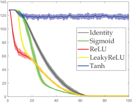
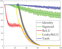
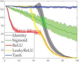
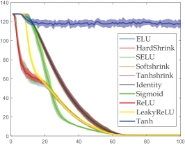
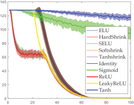
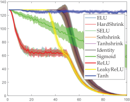
Theorem 1 shows that if we simply increase the depth based on GCN architecture, the extracted features will at most encode stationary information of graph structure and lose all the information in node features. In addition, from the proof we see that the point-wise ReLU transformation is a conspirator. Theorem 2 tells us that Tanh is better in keeping linear independence among column features. We design a numerical experiment on synthetic data (see Appendix) to test, under a 100-layer GCN architecture, how activation functions affect the rank of the output in each hidden layer during the feed-forward process. As Figure 1(a) shows, the rank of hidden features decreases rapidly with ReLU, while having little fluctuation under Tanh, and even the identity function performs better than ReLU (see Appendix for more comparisons). So we propose to replace ReLU by Tanh.
4 Spectral Graph Convolution and Block Krylov Subspace Methods
4.1 Notation and Backgrounds
Let be a block vector subspace of containing the identity matrix that is closed under matrix multiplication and transposition. We define an inner product in the block vector space as follows [10],
Definition 1
A mapping from to is called a block inner product onto if it satisfies the following conditions for all and :
-
1.
-linearity: and
-
2.
symmetry:
-
3.
definiteness: is positive definite if has full rank, and if and only if
There are mainly three ways to define , we use the classical one: and . We define a block vector subspace of , which will be used later.
Definition 2
Given a set of block vectors , the -span of is defined as
Given the above definition, the order- block Krylov subspace with respect to , and can be defined as . The corresponding block Krylov matrix is defined as .
4.2 Spectral Graph Convolution in Block Krylov Subspace Form
In this section, we will show that any graph convolution with well-defined analytic spectral filter defined on can be written as the product of a block Krylov matrix with a learnable parameter matrix in a specific form.
For any real analytic scalar function , its power series expansion around center 0 is
where is the radius of convergence. We can define a filter by . Let denote the spectrum radius of and suppose . The spectral filter can be defined as
According to the definition of spectral graph convolution in (1), graph signal is filtered by in the following way,
where and . It is easy to see that is a block Krylov matrix and Range() Range(). We know that there exists a smallest such that [12, 10]
| (4) |
i.e. for any , . depends on and , so we will write it as later, yet here we still use for simplicity. From (4), the convolution can be written as
| (5) |
where are parameter matrix blocks and under classical definition of inner product. Then
| (6) |
where . The essential number of learnable parameters is .
4.3 Deep GCN in Block Krylov Subspace Form
Since the spectral graph convolution can be simplified as (5)(6), we can build deep GCN in the following way.
Suppose we have a sequence of analytic spectral filters and a sequence of point-wise nonlinear activation functions . Then,
| (7) |
Let us define and . Then . From (6)(7), we have an iterative relation that where . It is easy to see that, when , (7) is fully connected network [20]; when , it is just GCN [17]; when is defined by Chebyshev polynomial [14], and under the global inner product, (7) is ChebNet [7].
4.4 Difficulties in Computation
In the last subsection, we gave a general form of deep GCN in block Krylov form. Following this idea, we can leverage the existing block Arnoldi (Lanczos) algorithm [10, 9] to compute orthogonal basis of and find . But there are some difficulties in practice:
-
1.
During the training phase, changes every time that parameters are updated. This makes become a variable and thus requires adaptive size for parameter matrices.
-
2.
For classical inner product, the factorization that is needed in block Arnoldi algorithm [10] is difficult to be put into backpropagation framework.
Although direct implementation of block Krylov methods in GCN is hard, it inspires us that if we have a good way to stack multi-scale information in each hidden layer, the network will have the ability to be extended to deep architectures. We propose a way to alleviate the difficulties in section 5.
5 Deep GCN Architectures
Upon the analyses in the last section, we propose two architectures: snowball and truncated Krylov. These methods concatenate multi-scale feature information in hidden layers differently while both having the potential to be scaled to deeper architectures.
5.1 Snowball
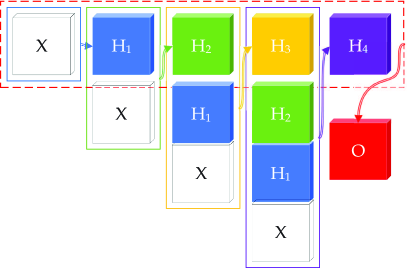
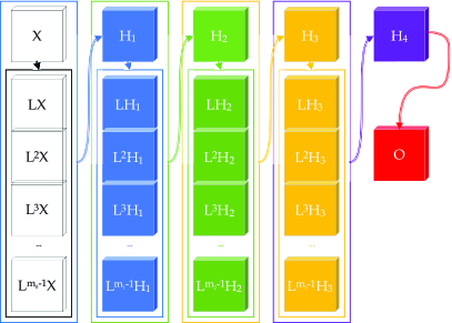
In order to concatenate multi-scale features together and get a richer representation for each node, we design a densely connected graph network (Figure 2(a)) as follows,
| (8) | ||||
where are learnable parameter matrices, is the number of output channels in layer ; are point-wise activation functions; is a classifier of any kind; . are extracted features. can be a fully connected neural network or even an identity layer with . When , and when , , which means that we project back onto graph Fourier basis which is necessary when graph structure encodes much information. Following this construction, we can stack all learned features as the input of the subsequent hidden layer, which is an efficient way to concatenate multi-scale information. The size of input will grow like a snowball and this construction is similar to DenseNet [16], which is designed for regular grids (images). Thus, some advantages of DenseNet are naturally inherited, e.g. alleviate the vanishing-gradient problem, encourage feature reuse, increase the variation of input for each hidden layer, reduce the number of parameters, strengthen feature propagation and improve model compactness.
5.2 Truncated Krylov
As stated in Section 4.4, the fact that is a variable makes GCN difficult to be merged into the block Krylov framework. But we can make a compromise and set as a hyperparameter. Then we can get a truncated block Krylov network (Figure 2(b)) as shown below,
| (9) | |||
where are learnable parameter matrices, and are activation functions, and .
There are many works on the analysis of error bounds of doing truncation in block Krylov methods [10]. But the results need many assumptions either on , e.g. is a standard Gaussian matrix [33], or on , e.g. some conditions on the smallest and largest eigenvalues of have to be satisfied [27]. Instead of doing truncation for a specific function or a fixed , we are dealing with variable during training. So we cannot put any restriction on and its relation to to get a practical error bound.
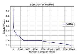
Here we would like to mention [24], which proposes to do low-rank approximation of by the Lanczos algorithm. The problem with this technique is that information in will be lost if is actually not low-rank. If we increase the Lanczos step to keep more information, it will hurt the efficiency of the algorithm. Since most of the graphs we are dealing with have sparse connectivity structures, they are actually not low-rank, e.g. Erdős-Rényi graph with [31] and Appendix \@slowromancapiv@. Thus we did not do low-rank approximation in our computations.
5.3 Equivalence of Linear Snowball GCN and Truncated Block Krylov Network
Under the snowball GCN architecture, the identity function outperforms ReLU as shown in Figure 1 and it is easier to train than Tanh. In this part, we will show that a multi-layer linear snowball GCN with identity function as , identity layer as and is equivalent to a 1-layer block Krylov network with identity layer , and a special parameter matrix.
5.4 Intuition behind Multi-scale Information Concatenation
For each node , denote as the set of its neighbors. Then can be interpreted as a weighted mean of and . If the networks goes deep as (3), becomes the weighted mean of and its hop neighbors (not exactly mean because we have ReLU in each layer). As the scope grows, the nodes in the same connected component tend to have the same (global) features, while losing their individual (local) features, which makes them indistinguishable. Although it is reasonable to assume that the nodes in the same cluster share many similar properties, it will be harmful if we ignore the "personal" differences between each node.
Therefore, to get a richer representation of each node, we propose to concatenate the multi-scale information together and the most naive architecture is the densely connected one. Truncated Krylov network works because in each layer , we start the concatenation from . By this way, the local information will not be diluted in each layer.
6 Experiments
We test linear snowball GCN (=identity, ), snowball GCN (=Tanh, =identity, ) and truncated block Krylov network (=Tanh, ) on public splits [36, 24] of Cora, Citeseer and PubMed111Source code to be found at https://github.com/PwnerHarry/Stronger_GCN, as well as several smaller splits to increase the difficulty of the tasks [24, 20, 30]. We compare against several methods which allow validation, including graph convolutional networks for fingerprint (GCN-FP) [8], gated graph neural networks (GGNN) [22], diffusion convolutional neural networks (DCNN) [1], Chebyshev networks (Cheby) [7], graph convolutional networks (GCN) [17], message passing neural networks (MPNN) [11], graph sample and aggregate (GraphSAGE) [13], graph partition neural networks (GPNN) [23], graph attention networks (GAT) [32], LanczosNet (LNet) [24] and AdaLanczosNet (AdaLNet) [24]. We also compare against some methods that do no use validation, including label propagation using ParWalks (LP) [34], Co-training [20], Self-training [20], Union [20], Intersection [20], GCN without validation [20], Multi-stage training [30], Multi-stage self-supervised (M3S) training [30], GCN with sparse virtual adversarial training (GCN-SVAT) [29] and GCN with dense virtual adversarial training (GCN-DVAT) [29].
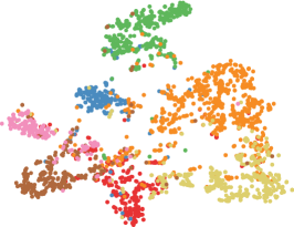
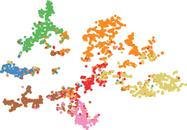
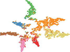
For each test case, we use the best hyperparameters to run independent times to get the average accuracy. The hyperparameters include learning rate and weight decay for the optimizer RMSprop or Adam, taking values in the intervals and , respectively, width of hidden layers taking value in the set , number of hidden layers in the set , dropout in , and the number of Krylov blocks taking value in . The hyperparameter values of the test cases will be presented in the appendix.
To get achieve good training, we use adaptive number of episodes (but no more than ): the early stopping counter is set to be 100.
We see that the proposed architectures achieve overwhelming performance in ALL test cases. It is particularly worth noting that when the training sets are small, the proposed architectures perform astonishingly better than the existing methods. From the t-SNE[25] visualization of the output layers in Figure 3, we see that the architectures extract good features with small training data, especially for truncated Krylov. What also impresses us is that linear Snowball GCN can achieve state-of-the-art performance with much less computational cost.
| Algorithms | Cora | CiteSeer | PubMed | |||||||||||||
| 0.5% | 1% | 2% | 3% | 4% | 5% | 0.5% | 1% | 2% | 3% | 4% | 5% | 0.03% | 0.05% | 0.1% | 0.3% | |
| LP | 56.4 | 62.3 | 65.4 | 67.5 | 69.0 | 70.2 | 34.8 | 40.2 | 43.6 | 45.3 | 46.4 | 47.3 | 61.4 | 66.4 | 65.4 | 66.8 |
| Cheby | 38.0 | 52.0 | 62.4 | 70.8 | 74.1 | 77.6 | 31.7 | 42.8 | 59.9 | 66.2 | 68.3 | 69.3 | 40.4 | 47.3 | 51.2 | 72.8 |
| Co-training | 56.6 | 66.4 | 73.5 | 75.9 | 78.9 | 80.8 | 47.3 | 55.7 | 62.1 | 62.5 | 64.5 | 65.5 | 62.2 | 68.3 | 72.7 | 78.2 |
| Self-training | 53.7 | 66.1 | 73.8 | 77.2 | 79.4 | 80.0 | 43.3 | 58.1 | 68.2 | 69.8 | 70.4 | 71.0 | 51.9 | 58.7 | 66.8 | 77.0 |
| Union | 58.5 | 69.9 | 75.9 | 78.5 | 80.4 | 81.7 | 46.3 | 59.1 | 66.7 | 66.7 | 67.6 | 68.2 | 58.4 | 64.0 | 70.7 | 79.2 |
| Intersection | 49.7 | 65.0 | 72.9 | 77.1 | 79.4 | 80.2 | 42.9 | 59.1 | 68.6 | 70.1 | 70.8 | 71.2 | 52.0 | 59.3 | 69.7 | 77.6 |
| MultiStage | 61.1 | 63.7 | 74.4 | 76.1 | 77.2 | 53.0 | 57.8 | 63.8 | 68.0 | 69.0 | 57.4 | 64.3 | 70.2 | |||
| M3S | 61.5 | 67.2 | 75.6 | 77.8 | 78.0 | 56.1 | 62.1 | 66.4 | 70.3 | 70.5 | 59.2 | 64.4 | 70.6 | |||
| GCN | 42.6 | 56.9 | 67.8 | 74.9 | 77.6 | 79.3 | 33.4 | 46.5 | 62.6 | 66.9 | 68.7 | 69.6 | 46.4 | 49.7 | 56.3 | 76.6 |
| GCN-SVAT | 43.6 | 53.9 | 71.4 | 75.6 | 78.3 | 78.5 | 47.0 | 52.4 | 65.8 | 68.6 | 69.5 | 70.7 | 52.1 | 56.9 | 63.5 | 77.2 |
| GCN-DVAT | 49 | 61.8 | 71.9 | 75.9 | 78.4 | 78.6 | 51.5 | 58.5 | 67.4 | 69.2 | 70.8 | 71.3 | 53.3 | 58.6 | 66.3 | 77.3 |
| linear Snowball | 69.5 | 74.1 | 79.4 | 80.4 | 81.3 | 82.2 | 56.8 | 65.4 | 68.8 | 71.0 | 72.2 | 72.2 | 64.1 | 69.5 | 72.9 | 79.3 |
| Snowball | 67.2 | 73.5 | 78.5 | 80.0 | 81.5 | 81.8 | 56.4 | 65.0 | 69.5 | 71.1 | 72.3 | 72.8 | 62.9 | 68.3 | 73.3 | 79.6 |
| truncated Krylov | 73.0 | 75.5 | 80.3 | 81.5 | 82.5 | 83.4 | 59.6 | 66.0 | 70.2 | 71.8 | 72.4 | 72.2 | 69.1 | 71.8 | 76.1 | 80.0 |
| For each (column), the greener the cell, the better the performance. The redder, the worse. If our methods achieve better performance than all others, the corresponding cell will be in bold. | ||||||||||||||||
| Algorithms | Cora | CiteSeer | PubMed | ||||||||
|---|---|---|---|---|---|---|---|---|---|---|---|
| 0.5% | 1% | 3% | 5.2% | 0.5% | 1% | 3.6% | 0.03% | 0.05% | 0.1% | 0.3% | |
| public | public | public | |||||||||
| Cheby | 33.9 | 44.2 | 62.1 | 78.0 | 45.3 | 59.4 | 70.1 | 45.3 | 48.2 | 55.2 | 69.8 |
| GCN-FP | 50.5 | 59.6 | 71.7 | 74.6 | 43.9 | 54.3 | 61.5 | 56.2 | 63.2 | 70.3 | 76.0 |
| GGNN | 48.2 | 60.5 | 73.1 | 77.6 | 44.3 | 56.0 | 64.6 | 55.8 | 63.3 | 70.4 | 75.8 |
| DCNN | 59.0 | 66.4 | 76.7 | 79.7 | 53.1 | 62.2 | 69.4 | 60.9 | 66.7 | 73.1 | 76.8 |
| MPNN | 46.5 | 56.7 | 72.0 | 78.0 | 41.8 | 54.3 | 64.0 | 53.9 | 59.6 | 67.3 | 75.6 |
| GraphSAGE | 37.5 | 49.0 | 64.2 | 74.5 | 33.8 | 51.0 | 67.2 | 45.4 | 53.0 | 65.4 | 76.8 |
| GAT | 41.4 | 48.6 | 56.8 | 83.0 | 38.2 | 46.5 | 72.5 | 50.9 | 50.4 | 59.6 | 79.0 |
| GCN | 50.9 | 62.3 | 76.5 | 80.5 | 43.6 | 55.3 | 68.7 | 57.9 | 64.6 | 73.0 | 77.8 |
| LNet | 58.1 | 66.1 | 77.3 | 79.5 | 53.2 | 61.3 | 66.2 | 60.4 | 68.8 | 73.4 | 78.3 |
| AdaLNet | 60.8 | 67.5 | 77.7 | 80.4 | 53.8 | 63.3 | 68.7 | 61.0 | 66.0 | 72.8 | 78.1 |
| linear Snowball | 70.0 | 73.1 | 81.0 | 83.2 | 59.4 | 65.9 | 73.5 | 68.1 | 70.0 | 73.8 | 79.2 |
| Snowball | 73.0 | 76.8 | 80.7 | 83.6 | 62.1 | 64.2 | 72.6 | 70.8 | 73.2 | 76.5 | 79.5 |
| truncated Krylov | 73.9 | 77.4 | 82.2 | 83.5 | 63.7 | 68.4 | 73.9 | 71.1 | 72.9 | 75.7 | 79.9 |
References
- [1] J. Atwood and D. Towsley. Diffusion-convolutional neural networks. arXiv, abs/1511.02136, 2015.
- [2] M. M. Bronstein, J. Bruna, Y. LeCun, A. Szlam, and P. Vandergheynst. Geometric deep learning: going beyond euclidean data. arXiv, abs/1611.08097, 2016.
- [3] J. Chen, T. Ma, and C. Xiao. Fastgcn: fast learning with graph convolutional networks via importance sampling. arXiv preprint arXiv:1801.10247, 2018.
- [4] J. Chen, J. Zhu, and L. Song. Stochastic training of graph convolutional networks with variance reduction. arXiv preprint arXiv:1710.10568, 2017.
- [5] R. R. Coifman and S. Lafon. Diffusion maps. Applied and computational harmonic analysis, 21(1):5–30, 2006.
- [6] R. R. Coifman and M. Maggioni. Diffusion wavelets. Applied and Computational Harmonic Analysis, 21(1):53–94, 2006.
- [7] M. Defferrard, X. Bresson, and P. Vandergheynst. Convolutional neural networks on graphs with fast localized spectral filtering. arXiv, abs/1606.09375, 2016.
- [8] D. K. Duvenaud, D. Maclaurin, J. Iparraguirre, R. Bombarell, T. Hirzel, A. Aspuru-Guzik, and R. P. Adams. Convolutional networks on graphs for learning molecular fingerprints. In Advances in neural information processing systems, pages 2224–2232, 2015.
- [9] A. Frommer, K. Lund, M. Schweitzer, and D. B. Szyld. The radau–lanczos method for matrix functions. SIAM Journal on Matrix Analysis and Applications, 38(3):710–732, 2017.
- [10] A. Frommer, K. Lund, and D. B. Szyld. Block Krylov subspace methods for functions of matrices. Electronic Transactions on Numerical Analysis, 47:100–126, 2017.
- [11] J. Gilmer, S. S. Schoenholz, P. F. Riley, O. Vinyals, and G. E. Dahl. Neural message passing for quantum chemistry. In Proceedings of the 34th International Conference on Machine Learning-Volume 70, pages 1263–1272. JMLR. org, 2017.
- [12] M. H. Gutknecht and T. Schmelzer. The block grade of a block krylov space. Linear Algebra and its Applications, 430(1):174–185, 2009.
- [13] W. L. Hamilton, R. Ying, and J. Leskovec. Inductive representation learning on large graphs. arXiv, abs/1706.02216, 2017.
- [14] D. K. Hammond, P. Vandergheynst, and R. Gribonval. Wavelets on graphs via spectral graph theory. Applied and Computational Harmonic Analysis, 30(2):129–150, 2011.
- [15] G. E. Hinton, S. Osindero, and Y.-W. Teh. A fast learning algorithm for deep belief nets. Neural computation, 18(7):1527–1554, 2006.
- [16] G. Huang, Z. Liu, L. Van Der Maaten, and K. Q. Weinberger. Densely connected convolutional networks. In Proceedings of the IEEE conference on computer vision and pattern recognition, pages 4700–4708, 2017.
- [17] T. N. Kipf and M. Welling. Semi-supervised classification with graph convolutional networks. arXiv, abs/1609.02907, 2016.
- [18] Y. LeCun, Y. Bengio, and G. Hinton. Deep learning. nature, 521(7553):436, 2015.
- [19] Y. LeCun, L. Bottou, Y. Bengio, P. Haffner, et al. Gradient-based learning applied to document recognition. Proceedings of the IEEE, 86(11):2278–2324, 1998.
- [20] Q. Li, Z. Han, and X. Wu. Deeper insights into graph convolutional networks for semi-supervised learning. arXiv, abs/1801.07606, 2018.
- [21] R. Li, S. Wang, F. Zhu, and J. Huang. Adaptive graph convolutional neural networks. In Thirty-Second AAAI Conference on Artificial Intelligence, 2018.
- [22] Y. Li, D. Tarlow, M. Brockschmidt, and R. Zemel. Gated graph sequence neural networks. arXiv preprint arXiv:1511.05493, 2015.
- [23] R. Liao, M. Brockschmidt, D. Tarlow, A. L. Gaunt, R. Urtasun, and R. Zemel. Graph partition neural networks for semi-supervised classification. arXiv preprint arXiv:1803.06272, 2018.
- [24] R. Liao, Z. Zhao, R. Urtasun, and R. S. Zemel. Lanczosnet: Multi-scale deep graph convolutional networks. arXiv, abs/1901.01484, 2019.
- [25] L. v. d. Maaten and G. Hinton. Visualizing data using t-sne. Journal of machine learning research, 9(Nov):2579–2605, 2008.
- [26] F. Monti, D. Boscaini, J. Masci, E. Rodola, J. Svoboda, and M. M. Bronstein. Geometric deep learning on graphs and manifolds using mixture model cnns. In Proceedings of the IEEE Conference on Computer Vision and Pattern Recognition, pages 5115–5124, 2017.
- [27] C. Musco, C. Musco, and A. Sidford. Stability of the lanczos method for matrix function approximation. In Proceedings of the Twenty-Ninth Annual ACM-SIAM Symposium on Discrete Algorithms, pages 1605–1624. Society for Industrial and Applied Mathematics, 2018.
- [28] D. I. Shuman, S. K. Narang, P. Frossard, A. Ortega, and P. Vandergheynst. The emerging field of signal processing on graphs: Extending high-dimensional data analysis to networks and other irregular domains. arXiv preprint arXiv:1211.0053, 2012.
- [29] K. Sun, H. Guo, Z. Zhu, and Z. Lin. Virtual adversarial training on graph convolutional networks in node classification. arXiv preprint arXiv:1902.11045, 2019.
- [30] K. Sun, Z. Zhu, and Z. Lin. Multi-stage self-supervised learning for graph convolutional networks. arXiv, abs/1902.11038, 2019.
- [31] L. V. Tran, V. H. Vu, and K. Wang. Sparse random graphs: Eigenvalues and eigenvectors. Random Structures & Algorithms, 42(1):110–134, 2013.
- [32] P. Veličković, G. Cucurull, A. Casanova, A. Romero, P. Lio, and Y. Bengio. Graph attention networks. arXiv, abs/1710.10903, 2017.
- [33] S. Wang, Z. Zhang, and T. Zhang. Improved analyses of the randomized power method and block lanczos method. arXiv preprint arXiv:1508.06429, 2015.
- [34] X.-M. Wu, Z. Li, A. M. So, J. Wright, and S.-F. Chang. Learning with partially absorbing random walks. In Advances in Neural Information Processing Systems, pages 3077–3085, 2012.
- [35] Z. Wu, S. Pan, F. Chen, G. Long, C. Zhang, and P. S. Yu. A comprehensive survey on graph neural networks. arXiv, abs/1901.00596, 2019.
- [36] Z. Yang, W. W. Cohen, and R. Salakhutdinov. Revisiting semi-supervised learning with graph embeddings. arXiv preprint arXiv:1603.08861, 2016.
- [37] S. Zhang, H. Tong, J. Xu, and R. Maciejewski. Graph convolutional networks: Algorithms, applications and open challenges. In International Conference on Computational Social Networks, pages 79–91. Springer, 2018.
Appendices
Appendix \@slowromancapi@: Proof of Theorem 1, 2
We extend Theorem 1 in [20] to a general diffusion operator in the following lemma.
-
Lemma1.
Suppose that a graph has connected components and the diffusion operator is defined as that in (2). has linearly independent eigenvectors corresponding to its largest eigenvalue . If has no bipartite components, then for any
(10) for some .
-
Lemma2.
Suppose we randomly sample under a continuous distribution. Suppose we have point-wise function , we have
Proof We generalize ReLU onto multi-dimensional case by applying it element-wise on every element of the matrix. Any can be represented as , where and are the nonnegative and nonpositive components of , respectively. We can see that . It is trivial when . We only discuss for all nonzero .
Suppose and are linearly independent (with probability ), then that . If that ReLU= ReLU, then and and the existence of this kind of has a nonzero probability (See Lemma 3); other than these cases, the independency will be kept after the ReLU transformation.
Suppose is linearly dependent of (with probability 0), i.e., that . If , we have and . Since ReLU=, ReLU=, then ReLU= ReLU. If , we have and . If that ReLU= ReLU, this means . This exists when and are linearly dependent, which only holds when . This happens with probability 0. Then, ReLU and ReLU will be independent. So whether ReLU keep the dependency between to vectors or not depends on the sign of . Thus, under the assumption, we have probability that ReLU keeps the dependency.
According to the discussion above, we have
Lemma proved.
-
Lemma3.
Suppose we randomly sample under a continuous distribution, then
Proof
where denotes degree of freedom. means that can at most have one dimension to be positive and there are out of hyperoctants that satisfies this condition. The set of that can make hold has an area of , i.e. when is in the same hyperoctant as . If lies in other hyperoctants, . And since , is just a low dimensional surface in with area 0.
- Theorem1.
Proof Upon the conclusions in Lemma 2-3, we have rankrank() with probability 1 and it is obvious rankrank(). Using these two inequality iteratively for (3), we have rank() rank(). Based on Lemma 1, we have probability 1 to get
where . Thus, rank()
-
Theorem2.
Suppose we randomly sample under a continuous distribution and we have the point-wise function , we have
Proof We first prove it for . It is trivial when have 0 elements.
Suppose are linearly dependent and all of their elements are nonzero. If and are still linearly dependent, we must have
This equation only have one solution
which means point-wise Tanh transformation will break the dependency of with probability 1.
If are linearly independent, suppose is a vector in , and the set of vectors in that can be transformed by point-wise Tanh to the same line as covers an area of probability 0. That is for any fixed , the solution of
covers an area of 0. Thus,
which means point-wise Tanh transformation will increase the independency between vectors in .
Similar to , suppose are linearly dependent, if all elements in are nonzero and and are still linearly dependent, we must have
The solution of any pair of equations covers an area of probability 0 in . Actually, this still holds when have some 0 elements, i.e. for any subset of the above equations, the area of the solution is still 0.
If are linearly independent, suppose is a vector in , and the space in that can be transformed by point-wise Tanh to the same line as covers an area of probability 0. Therefore, Lemma 2 still holds in .
Appendix \@slowromancapii@: Numerical Experiments on Synthetic Data
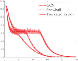
The goal of the experiments is to test which network structure with which kind of activation function has the potential to be extended to deep architecture. We measure this potential by the numerical rank of the output features in each hidden layer of the networks using synthetic data. The reason of choosing this measure can be explained by Theorem 3. We build the certain networks with depth 100 and the data is generated as follows.
We first randomly generate edges of an Erdős-Rényi graph , i.e. the existence of the edge between any pair of nodes is a Bernoulli random variable with . Then, we construct the corresponding adjacency matrix of the graph which is a matrix. We generate a feature matrix and each of its element is drawn from . We normalize and as [17] and abuse the notation to denote the normalized matrices. We keep 3 blocks in each layer of truncated block Krylov network. The number of input channel in each layer depends on the network structures and the number of output channel is set to be 128 for all networks. Each element in every parameter matrix is randomly sampled from and the size is . With the synthetic , we simulate the feedforward process according to the network architecture and collect the numerical rank (at most 128) of the output in each of the 100 hidden layers. For each activation function under each network architecture, we repeat the experiments for 20 times and plot the mean results with standard deviation bars.
Appendix \@slowromancapiii@: Rank Comparison of Activation Functions and Networks
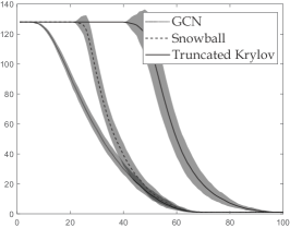
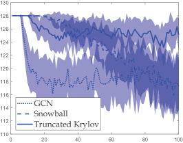
Appendix \@slowromancapiv@: Spectrum of the Datasets
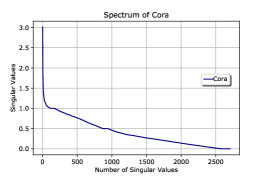
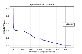
Appendix \@slowromancapv@: Experiment Settings and Hyperparameters
The so-called public splits in [24] and the setting that randomly sample 20 instances for each class as labeled data in [36] is actually the same. Most of the results for the algorithms with validation are cited from [24], where they are reproduced with validation. However, some of them actually do not use validation in original papers and can achieve better results. In the paper, We compare with their best results.
We use NVIDIA apex amp mixed-precision plugin for PyTorch to accelerate our experiments. Most of the results were obtained from NVIDIA V100 clusters on Beluga of Compute-Canada, with minor part of them obtained from NVIDIA K20, K80 clusters on Helios Compute-Canada. The hyperparameters are searched using Bayesian optimization.
A useful tip is the smaller your training set is, the larger dropout probability should be set and the larger early stopping you should have.
Table 4 and Table 3 shows the hyperparameters to achieve the performance in the experiments, for cases without and with validation, respectively. When conducting the hyperparameter search, we encounter memory problems: current GPUs cannot afford deeper and wider structures. But we do observe better performance with the increment of the network size. It is expected to achieve better performance with more advanced deep learning devices.
| Architecture | Dataset | Percentage | Accuracy | Corresponding Hyperparameters | ||||||
|---|---|---|---|---|---|---|---|---|---|---|
| Ours | SOTA | lr | weight_decay | hidden | layers/n_blocks | dropout | optimizer | |||
| linear Snowball | Cora | 0.5% | 69.99 | 60.8 | 1.0689E-03 | 1.4759E-02 | 128 | 6 | 0.66987 | RMSprop |
| 1% | 73.10 | 67.5 | 1.4795E-03 | 2.3764E-02 | 128 | 9 | 0.64394 | RMSprop | ||
| 3% | 80.96 | 77.7 | 2.6847E-03 | 5.1442E-03 | 64 | 9 | 0.23648 | RMSprop | ||
| 5.2% (public) | 83.19 | 83.0 | 1.6577E-04 | 1.8606E-02 | 1024 | 3 | 0.65277 | RMSprop | ||
| CiteSeer | 0.5% | 59.41 | 53.8 | 4.9284E-04 | 6.9420E-03 | 512 | 11 | 0.90071 | RMSprop | |
| 1% | 65.85 | 63.3 | 3.2628E-03 | 1.6374E-02 | 512 | 3 | 0.97331 | RMSprop | ||
| 3.6% (public) | 73.54 | 72.5 | 2.8218E-03 | 1.9812E-02 | 5000 | 1 | 0.98327 | Adam | ||
| Pubmed | 0.03% | 68.12 | 61.0 | 2.1124E-03 | 4.4161E-02 | 128 | 7 | 0.78683 | RMSprop | |
| 0.05% | 70.04 | 68.8 | 4.9982E-03 | 2.6460E-02 | 128 | 4 | 0.86788 | RMSprop | ||
| 0.1% | 73.83 | 73.4 | 1.2462E-03 | 4.9303E-02 | 128 | 6 | 0.3299 | RMSprop | ||
| 0.3% (public) | 79.23 | 79.0 | 2.4044E-03 | 2.3157E-02 | 4000 | 1 | 0.98842 | Adam | ||
| Snowball | Cora | 0.5% | 72.96 | 60.8 | 2.3228E-04 | 2.1310E-02 | 950 | 7 | 0.88945 | RMSprop |
| 1% | 76.76 | 67.5 | 1.5483E-04 | 1.3963E-02 | 250 | 15 | 0.55385 | RMSprop | ||
| 3% | 80.72 | 77.7 | 1.6772E-03 | 1.0725E-02 | 64 | 14 | 0.80611 | RMSprop | ||
| 5.2% (public) | 83.60 | 83.0 | 1.2994E-05 | 9.4469E-03 | 5000 | 3 | 0.025052 | RMSprop | ||
| CiteSeer | 0.5% | 62.05 | 53.8 | 2.0055E-03 | 3.1340E-02 | 512 | 5 | 0.88866 | RMSprop | |
| 1% | 64.23 | 63.3 | 1.8759E-03 | 9.3636E-03 | 128 | 7 | 0.77334 | RMSprop | ||
| 3.6% (public) | 72.61 | 72.5 | 2.5527E-03 | 6.2812E-03 | 256 | 1 | 0.56755 | RMSprop | ||
| Pubmed | 0.03% | 70.78 | 61.0 | 1.1029E-03 | 1.8661E-02 | 100 | 15 | 0.83381 | RMSprop | |
| 0.05% | 73.23 | 68.8 | 3.7159E-03 | 2.2088E-02 | 400 | 9 | 0.9158 | RMSprop | ||
| 0.1% | 76.52 | 73.4 | 4.9106E-03 | 3.0777E-02 | 100 | 15 | 0.79133 | RMSprop | ||
| 0.3% (public) | 79.54 | 79.0 | 4.9867E-03 | 3.5816E-03 | 3550 | 1 | 0.98968 | Adam | ||
| truncated Krylov | Cora | 0.5% | 73.89 | 60.8 | 1.6552E-04 | 4.4330E-02 | 4950 | 27 | 0.97726 | Adam |
| 1% | 77.38 | 67.5 | 2.8845E-04 | 4.8469E-02 | 4950 | 30 | 0.93928 | Adam | ||
| 3% | 82.23 | 77.7 | 8.6406E-04 | 4.0126E-03 | 2950 | 16 | 0.98759 | Adam | ||
| 5.2% (public) | 83.51 | 83.0 | 1.0922E-03 | 3.5966E-02 | 1950 | 10 | 0.98403 | Adam | ||
| CiteSeer | 0.5% | 63.65 | 53.8 | 2.8208E-03 | 4.3395E-02 | 1150 | 30 | 0.92821 | Adam | |
| 1% | 68.36 | 63.3 | 3.9898E-03 | 3.8525E-03 | 100 | 27 | 0.71951 | Adam | ||
| 3.6% (public) | 73.89 | 72.5 | 1.8292E-03 | 4.2295E-02 | 600 | 11 | 0.98865 | Adam | ||
| Pubmed | 0.03% | 71.11 | 61.0 | 3.6759E-03 | 1.2628E-02 | 512 | 8 | 0.95902 | RMSprop | |
| 0.05% | 72.86 | 68.8 | 4.0135E-03 | 4.8831E-02 | 4250 | 5 | 0.95911 | Adam | ||
| 0.1% | 75.68 | 73.4 | 4.7562E-03 | 3.7134E-02 | 950 | 7 | 0.96569 | Adam | ||
| 0.3% (public) | 79.88 | 79.0 | 3.9673E-04 | 2.2931E-02 | 1900 | 4 | 0.000127 | Adam | ||
| Architecture | Dataset | Percentage | Accuracy | Correspondong Hyperparameters | ||||||
|---|---|---|---|---|---|---|---|---|---|---|
| Ours | SOTA | lr | weight_decay | hidden | layers/n_blocks | dropout | Optimizer | |||
| linear Snowball | Cora | 0.5% | 69.53 | 61.5 | 4.4438E-05 | 1.7409E-02 | 550 | 12 | 0.007753 | Adam |
| 1% | 74.12 | 69.9 | 1.0826E-03 | 3.3462E-03 | 1250 | 3 | 0.50426 | Adam | ||
| 2% | 79.43 | 75.9 | 2.4594E-06 | 9.6734E-03 | 1650 | 12 | 0.34073 | Adam | ||
| 3% | 80.41 | 78.5 | 2.8597E-05 | 3.4732E-02 | 900 | 15 | 0.039034 | Adam | ||
| 4% | 81.3 | 80.4 | 3.6830E-05 | 1.5664E-02 | 3750 | 4 | 0.93797 | Adam | ||
| 5% | 82.19 | 81.7 | 5.8323E-06 | 8.5940E-03 | 2850 | 5 | 0.14701 | Adam | ||
| CiteSeer | 0.5% | 56.76 | 56.1 | 4.5629E-03 | 2.0106E-03 | 300 | 3 | 0.038225 | Adam | |
| 1% | 65.44 | 62.1 | 3.5530E-05 | 4.9935E-02 | 600 | 6 | 0.03556 | Adam | ||
| 2% | 68.78 | 68.6 | 6.1176E-06 | 3.0101E-02 | 1950 | 3 | 0.040484 | Adam | ||
| 3% | 71 | 70.3 | 2.1956E-05 | 4.3569E-02 | 3350 | 3 | 0.30207 | Adam | ||
| 4% | 72.23 | 70.8 | 9.1952E-05 | 4.6407E-02 | 3350 | 2 | 0.018231 | Adam | ||
| 5% | 72.21 | 71.3 | 3.7173E-03 | 1.9605E-03 | 2950 | 1 | 0.96958 | Adam | ||
| Pubmed | 0.03% | 64.133 | 62.2 | 1.0724E-03 | 8.1097E-03 | 64 | 4 | 0.8022 | RMSProp | |
| 0.05% | 69.48 | 68.3 | 1.5936E-03 | 3.0236E-03 | 6 | 10 | 0.73067 | RMSProp | ||
| 0.1% | 72.93 | 72.7 | 4.9733E-03 | 1.3744E-03 | 128 | 3 | 0.91214 | RMSProp | ||
| 0.3% | 79.33 | 79.2 | 1.7998E-03 | 9.6753E-04 | 512 | 1 | 0.97483 | RMSProp | ||
| Snowball | Cora | 0.5% | 67.15 | 61.5 | 9.8649E-04 | 1.0305E-02 | 1600 | 3 | 0.92785 | Adam |
| 1% | 73.47 | 69.9 | 1.4228E-04 | 1.3472E-02 | 100 | 13 | 0.68601 | Adam | ||
| 2% | 78.54 | 75.9 | 5.7111E-06 | 1.5544E-02 | 600 | 13 | 0.022622 | Adam | ||
| 3% | 79.97 | 78.5 | 4.0278E-05 | 2.7287E-02 | 4350 | 5 | 0.57173 | Adam | ||
| 4% | 81.49 | 80.4 | 1.4152E-05 | 2.3359E-02 | 2500 | 13 | 0.018578 | Adam | ||
| 5% | 81.82 | 81.7 | 1.2621E-03 | 1.5323E-02 | 3550 | 2 | 0.87352 | Adam | ||
| CiteSeer | 0.5% | 56.39 | 56.1 | 2.6983E-03 | 2.5370E-02 | 300 | 6 | 0.82964 | Adam | |
| 1% | 65.04 | 62.1 | 1.6982E-03 | 1.5473E-02 | 2150 | 2 | 0.98611 | Adam | ||
| 2% | 69.48 | 68.6 | 9.7299E-05 | 4.9675E-02 | 2150 | 3 | 0.71216 | Adam | ||
| 3% | 71.09 | 70.3 | 1.7839E-04 | 3.0874E-02 | 2150 | 2 | 0.16549 | Adam | ||
| 4% | 72.32 | 70.8 | 5.6575E-05 | 3.5949E-02 | 4800 | 2 | 0.012576 | Adam | ||
| 5% | 72.8 | 71.3 | 2.8643E-04 | 1.6399E-02 | 2000 | 2 | 0.37308 | Adam | ||
| Pubmed | 0.03% | 62.94 | 62.2 | 1.2700E-03 | 1.4159E-03 | 128 | 4 | 0.76848 | RMSProp | |
| 0.05% | 68.31 | 68.3 | 1.1224E-03 | 9.9166E-05 | 256 | 3 | 0.85496 | RMSProp | ||
| 0.1% | 73.29 | 72.7 | 6.0506E-04 | 1.0303E-03 | 256 | 2 | 0.97988 | RMSProp | ||
| 0.3% | 79.63 | 79.2 | 1.1416E-03 | 6.1543E-04 | 128 | 1 | 0.989 | RMSProp | ||
| truncated Krylov | Cora | 0.5% | 72.96 | 61.5 | 3.3276E-03 | 1.0496E-04 | 128 | 18 | 0.76012 | RMSProp |
| 1% | 75.52 | 69.9 | 7.4797E-04 | 9.1736E-03 | 2048 | 20 | 0.98941 | RMSProp | ||
| 2% | 80.31 | 75.9 | 1.7894E-04 | 1.1079E-02 | 4096 | 16 | 0.97091 | RMSProp | ||
| 3% | 81.54 | 78.5 | 4.3837E-04 | 2.6958E-03 | 512 | 17 | 0.96643 | RMSProp | ||
| 4% | 82.47 | 80.4 | 3.6117E-03 | 4.1040E-04 | 64 | 25 | 0.021987 | RMSProp | ||
| 5% | 83.36 | 81.7 | 1.0294E-03 | 5.3882E-04 | 256 | 23 | 0.028392 | RMSProp | ||
| CiteSeer | 0.5% | 59.6 | 56.1 | 1.9790E-03 | 4.0283E-04 | 16 | 20 | 0.007761 | RMSProp | |
| 1% | 65.95 | 62.1 | 7.8506E-04 | 8.2432E-03 | 64 | 24 | 0.28159 | RMSProp | ||
| 2% | 70.23 | 68.6 | 5.4517E-04 | 1.0818E-02 | 256 | 12 | 0.27027 | RMSProp | ||
| 3% | 71.81 | 70.3 | 1.4107E-04 | 5.0062E-03 | 1024 | 9 | 0.57823 | RMSProp | ||
| 4% | 72.36 | 70.8 | 4.8864E-06 | 1.8038E-02 | 4096 | 12 | 0.11164 | RMSProp | ||
| 5% | 72.24 | 71.3 | 2.1761E-03 | 1.1753E-02 | 5000 | 8 | 0.71473 | Adam | ||
| Pubmed | 0.03% | 69.07 | 62.2 | 6.8475E-04 | 2.8822E-02 | 4096 | 7 | 0.97245 | RMSProp | |
| 0.05% | 71.77 | 68.3 | 2.3342E+04 | 2.2189E-03 | 1024 | 8 | 0.93694 | RMSProp | ||
| 0.1% | 76.07 | 72.7 | 4.2629E-04 | 4.1339E-03 | 2048 | 8 | 0.98914 | RMSProp | ||
| 0.3% | 80.04 | 79.2 | 2.2602E-04 | 3.3626E-02 | 2000 | 7 | 0.070573 | Adam | ||