Physics Enhanced Data-Driven Models with Variational Gaussian Processes

Abstract

Centuries of development in natural sciences and mathematical modeling provide valuable domain expert knowledge that has yet to be explored for the development of machine learning models. When modeling complex physical systems, both domain knowledge and data provide necessary information about the system. In this paper, we present a data-driven model that takes advantage of partial domain knowledge in order to improve generalization and interpretability. The presented approach, which we call EVGP (Explicit Variational Gaussian Process), has the following advantages: 1) using available domain knowledge to improve the assumptions (inductive bias) of the model, 2) scalability to large datasets, 3) improved interpretability. We show how the EVGP model can be used to learn system dynamics using basic Newtonian mechanics as prior knowledge. We demonstrate how the addition of prior domain-knowledge to data-driven models outperforms purely data-driven models.

=-15pt

I Introduction

For centuries, scientists and engineers have worked on creating mathematical abstractions of real world systems. This principled modeling approach provides a powerful toolbox to derive white-box models that we can use to understand and analyze physical systems. However, as the complexity of physical systems grow, deriving detailed principled models becomes an expensive and tedious task that requires highly experienced scientists and engineers. Moreover, incorrect assumptions leads to inaccurate models that are unable to represent the real system.

Data-driven black-box models provide an appealing alternative modeling approach that requires little to none domain knowledge. These models are fit to data extracted from the real system, minimizing the problems derived from incorrect assumptions. However, using data-driven models while completely ignoring domain knowledge may lead to models that do not generalize well and are hard to understand. Completely black-box approaches ignore the structure of the problem, wasting resources (szegedy2015going, ) and making the model less explainable (adadi2018peeking, ).

Gray-box models combine domain knowledge and data as both provide important and complementary information about the system. Domain knowledge can be used to construct a set of basic assumptions about the system, giving the data-driven model a baseline to build upon. Data can be used to fill the gaps in knowledge and model complex relations that were not considered by the domain expert.

In this paper, we explore an approach for embedding domain knowledge into a data-driven model in order to improve generalization and interpretability. The presented gray-box model, which we called EVGP (Explicit Variational Gaussian Process), is a scalable approximation of a sparse Gaussian Process (GP) that uses domain knowledge to define the prior distribution of the GP. In this paper domain knowledge is extracted from physics-based knowledge, however the EVGP can be applied to any domain.

Figure 1: EVGP: Variational Gaussian-Process with explicit features

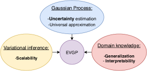
The work on this paper has three cornerstones (Fig. 1): 1) Gaussian processes are used for learning complex non-linear behavior from data and model uncertainty, 2) Partial domain knowledge is used as prior in order to improve inductive bias, 3) Variational Inference provides advantageous scalability to large datasets. Inductive bias refers to the assumptions made by the model when doing predictions over inputs that have not been observed. The presented approach provides uncertainty estimations which are fundamental in order to avoid the risk associated with overconfidence in unexplored areas (frigola2014variational, ) and warns the user of possible incorrect estimations (marino2017data, ).

The work in this paper is highly applicable when: 1) modeling physical systems with uncertainty estimations, 2) partial domain knowledge of the system is available, 3) large quantities of data are available. The aim is to help the engineer and take advantage of available knowledge without requiring the derivation of complex and detailed models. Instead, an engineer only has to provide simple, partially formed, models and the EVGP takes care of filling the gaps in knowledge. We show how the EVGP model can be used to learn system dynamics using basic physics laws as prior knowledge.

The contributions of this paper are:

• We present a stochastic data-driven model enhanced with domain knowledge to improve model accuracy using less amount of data when compared with fully data-driven approaches.

• The presented approach uses very simple priors, demonstrating that accuracy gets improved by incorporating priors derived from heavily simplified physics.

• Scalability to handle large datasets is achieved by using the sparse variational framework.

• Interpretability is exemplified using the posterior distribution of trainable parameters, i.e. the value of the model parameters after training.

Our objective is to evaluate the benefits of including partially defined (imperfect) models as domain-knowledge to data-driven models. As such, our experiments compare the performance of the EVGP approach with respect to fully data-driven (black-box) models to evaluate the benefits of the proposed approach.

The rest of the paper is organized as follows: section II presents the proposed EVGP approach; section III presents a set of priors derived from simplified Newtonian dynamics for the EVGP model; section IV presents the experimental section where we compare the EVGP with fully data-driven models; section V presents the related work; section VI concludes the paper.

II EVGP approach - variational GP using explicit features

Figure 2: Illustration of the EVGP model.

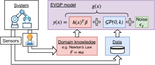
The novel EVGP approach presented in this paper is designed to solve regression problems under uncertainty. Figure 2 offers a visual representation of the approach.

Given a dataset ${\cal D}=({\boldsymbol{x}}^{(i)},{\boldsymbol{y}}^{(i)})$ composed of input/output pairs of samples $\left({\boldsymbol{x}}^{(i)},{\boldsymbol{y}}^{(i)}\right)$, we would like to obtain a predictive distribution $p({\boldsymbol{y}}|{\boldsymbol{x}},{\cal D})$ that estimates the value of the output ${\boldsymbol{y}}$ for a given input ${\boldsymbol{x}}$. The EVGP model approximates $p({\boldsymbol{y}}|{\boldsymbol{x}},{\cal D})$ using variational Inference. The EVGP is defined as a distribution $p({\boldsymbol{y}}|{\boldsymbol{x}},w)$ where $w$ are a set of parameters with prior distribution $p(w)$.

In the following sections we describe in detail: A) the EVGP model approach, B) the variational loss function used to train the model, C) the predictive distribution that approximates $p({\boldsymbol{y}}|{\boldsymbol{x}},{\cal D})$.

II-A EVGP Model Definition

The EVGP model takes the following form:

$$y=g({\boldsymbol{x}})+\epsilon_{y};\;\;\;{g\left({\boldsymbol{x}}\right)}={h\left({\boldsymbol{x}}\right)}^{T}{\boldsymbol{\beta}}+{f\left({\boldsymbol{x}}\right)}$$ (1)

where ${f\left({\boldsymbol{x}}\right)}\sim{\cal GP}\left(0,{k\left({\boldsymbol{x}},{\boldsymbol{x}}^{\prime}\right)}\right)$ is a Gaussian process with kernel $k$, $\epsilon_{y}\sim{\cal N}\left(0,{\boldsymbol{\Sigma}}_{y}\right)$ is the observation noise and $g({\boldsymbol{x}})$ is the denoised prediction for the input ${\boldsymbol{x}}$. Figure 2 offers a visual representation of the model. The following is the description of the main components of the EVGP model:

• Domain knowledge is embedded in the explicit function ${h\left({\boldsymbol{x}}\right)}^{T}{\boldsymbol{\beta}}$, parameterized by ${\boldsymbol{\beta}}$. The function ${h\left({\boldsymbol{x}}\right)}$ describes a set of explicit features (hence the name of our method) provided by the domain expert. ${\boldsymbol{\beta}}$ is modeled using a normal distribution with a prior that is also extracted from domain knowledge. In this paper, $h({\boldsymbol{x}})^{T}{\boldsymbol{\beta}}$ is derived from partially defined Newtonian mechanics.

• The Gaussian Process $f({\boldsymbol{x}})$ adds the ability to learn complex non-linear relations that ${h\left({\boldsymbol{x}}\right)}^{T}{\boldsymbol{\beta}}$ is unable to capture.

Given a dataset ${\cal D}$, the exact predictive distribution $p(y|x,{\cal D})$ for the model in Eq. 1 is described in (rasmussen2004gaussian, ). For the rest of the paper, we refer to the exact distribution as EGP. Computing the EGP predictive distribution has a large computational cost and does not scale well for large datasets. To alleviate this problem, sparse approximation methods (quinonero2005unifying, ) use a small set of $m$ inducing points $({\boldsymbol{f}}_{m},{\boldsymbol{X}}_{m})$ (trainable parameters) instead of the entire dataset to approximate the predictive distribution.

In order to construct a sparse approximation for the model in Eq. 1, we use a set of $m$ inducing points $({\boldsymbol{f}}_{m},{\boldsymbol{X}}_{m})$ as parameters that will be learned from data. Given $({\boldsymbol{f}}_{m},{\boldsymbol{X}}_{m})$ and a set of test points $({\boldsymbol{g}},{\boldsymbol{X}})$, the prior distribution of the model can be expressed as follows:

$$\begin{bmatrix}{\boldsymbol{g}}_{m}\mid{\boldsymbol{\beta}}\\ \;\;{\boldsymbol{g}}\mid{\boldsymbol{\beta}}\end{bmatrix}\sim{\cal N}\left(\begin{bmatrix}{\boldsymbol{H}}_{m}{\boldsymbol{\beta}}\\ {\boldsymbol{H}}_{x},{\boldsymbol{\beta}}\end{bmatrix},\begin{bmatrix}{\boldsymbol{K}}_{mm}&{\boldsymbol{K}}_{m{\boldsymbol{x}}}\\ {\boldsymbol{K}}_{{\boldsymbol{x}}m}&{\boldsymbol{K}}_{{\boldsymbol{x}}{\boldsymbol{x}}}\end{bmatrix}\right);$$

$${\boldsymbol{H}}_{m} ={h\left({\boldsymbol{X}}_{m}\right)};\;\;\;{\boldsymbol{H}}_{x}={h\left({\boldsymbol{X}}\right)}$$

$${\boldsymbol{g}}_{m} =h({\boldsymbol{X}}_{m}){\boldsymbol{\beta}}+{\boldsymbol{f}}_{m}$$

where ${\boldsymbol{X}}$ denotes the data matrix, where each row represents an individual sample. The rows of ${\boldsymbol{H}}_{x}$ represent the value of the function $h()$ applied to the real samples ${\boldsymbol{X}}$. The rows of ${\boldsymbol{H}}_{m}$ represent the value of the function $h()$ applied to the inducing (learned) points ${\boldsymbol{X}}_{m}$. Using the conditional rule for multivariate Gaussian distributions, we obtain the definition of the denoised sparse EVGP model:

$${p\left({\boldsymbol{g}}\mid{\boldsymbol{X}},\omega\right)}\sim {\cal N}\left({\boldsymbol{H}}_{x}{\boldsymbol{\beta}}+{\boldsymbol{\mu}}_{{\boldsymbol{f}}\mid\omega},{\boldsymbol{\Sigma}}_{{\boldsymbol{f}}\mid\omega}\right)$$ (2)

where $\omega={\left\{{\boldsymbol{f}}_{m},{\boldsymbol{\beta}}\right\}}$ are the parameters of our model, ${\boldsymbol{\mu}}_{{\boldsymbol{f}}\mid\omega}={\boldsymbol{K}}_{{\boldsymbol{x}}m}{\boldsymbol{K}}_{mm}^{-1}{\boldsymbol{f}}_{m}$, and ${\boldsymbol{\Sigma}}_{{\boldsymbol{f}}\mid\omega}={\boldsymbol{K}}_{{\boldsymbol{x}}{\boldsymbol{x}}}-{\boldsymbol{K}}_{{\boldsymbol{x}}m}{\boldsymbol{K}}_{mm}^{-1}{\boldsymbol{K}}_{mx}$. Equation 2 defines our scalable EVGP model. In following sections we give prior distributions to the parameters $\omega$ and perform approximate Bayesian inference. Note that Eq. 2 is also conditioned on ${\boldsymbol{X}}_{m}$, however we do not indicate this explicitly in order to improve readability.

II-B Variational Loss

In this section we present the loss function that we use to fit our model. In this paper we follow a variational Bayesian approach (see Appendix A for a brief overview). Given a training dataset ${\cal D}$ and a prior distribution $p(\omega)$, we wish to approximate the posterior distribution $p(\omega|{\cal D})$. The posterior of $\omega$ is approximated using a variational distribution ${p_{\phi}\left(w\right)}\approx p(\omega|{\cal D})$ parameterized by $\phi$. For the EVGP parameters $\omega={\left\{{\boldsymbol{f}}_{m},{\boldsymbol{\beta}}\right\}}$, we use the following variational posterior distributions:

$${p_{\phi}\left({\boldsymbol{f}}_{m}\right)}={\cal N}\left({\boldsymbol{f}}_{m}|{\boldsymbol{a}},{\boldsymbol{A}}\right);\;\;\;{p_{\phi}\left({\boldsymbol{\beta}}\right)}={\cal N}\left({\boldsymbol{\beta}}|{\boldsymbol{b}},{\boldsymbol{B}}\right)$$

The prior-distributions for $\omega$ are also defined as multivariate normal distributions:

$${p\left({\boldsymbol{f}}_{m}\right)}={\cal N}\left({\boldsymbol{f}}_{m}\mid 0,{\boldsymbol{K}}_{mm}\right);\;\;\;{p\left({\boldsymbol{\beta}}\right)}={\cal N}\left({\boldsymbol{\beta}}\mid{\boldsymbol{\mu}}_{\beta},{\boldsymbol{\Sigma}}_{\beta}\right)$$

these prior distributions represent our prior knowledge, i.e. our knowledge before looking at the data.

Given the training dataset ${\cal D}=({\boldsymbol{y}},{\boldsymbol{X}})$, the parameters $\phi$ of ${p_{\phi}\left(\omega\right)}$ are learned by minimizing the negative Evidence Lower Bound (ELBO). For the EVGP, the negative ELBO takes the following form:

$${\mathcal{L}\left(\phi\right)}= -\log{\cal N}\left({\boldsymbol{y}}\mid{\boldsymbol{H}}_{x}{\boldsymbol{b}}+{\boldsymbol{K}}_{xm}{\boldsymbol{K}}_{mm}^{-1}{\boldsymbol{a}},{\boldsymbol{\Sigma}}_{y}\right)$$

$$+\dfrac{1}{2}\left[\text{Tr}\left({\boldsymbol{M}}_{1}{\boldsymbol{A}}\right)+\text{Tr}\left({\boldsymbol{M}}_{2}{\boldsymbol{B}}\right)+\text{Tr}\left({\boldsymbol{\Sigma}}_{y}^{-1}{\boldsymbol{\Sigma}}_{{\boldsymbol{f}}\mid\omega}\right)\right]+\mathcal{L}_{KL}$$ (3)

where ${\boldsymbol{M}}_{1}=\left({\boldsymbol{K}}_{mm}^{-1}{\boldsymbol{K}}_{mx}\right){\boldsymbol{\Sigma}}_{y}^{-1}\left({\boldsymbol{K}}_{xm}{\boldsymbol{K}}_{mm}^{-1}\right)$, and ${\boldsymbol{M}}_{2}={\boldsymbol{H}}_{x}^{T}{\boldsymbol{\Sigma}}_{y}^{-1}{\boldsymbol{H}}_{x}$. The term $\mathcal{L}_{KL}$ is the KL-divergence between the posterior and prior distributions for the parameters:

$$\mathcal{L}_{KL}= D_{KL}\left({\cal N}\left({\boldsymbol{a}},{\boldsymbol{A}}\right)\mid\mid{\cal N}\left(0,{\boldsymbol{K}}_{mm}\right)\right)$$

$$+D_{KL}\left({\cal N}\left({\boldsymbol{b}},{\boldsymbol{B}}\right)\mid\mid{\cal N}\left({\boldsymbol{\mu}}_{\beta},{\boldsymbol{\Sigma}}_{\beta}\right)\right)$$

A detailed derivation of the variational loss in Eq. 3 is presented in Appendix B. The negative ELBO (Eq. 3) serves as our loss function to learn the parameters $\phi$ given the training dataset ${\boldsymbol{y}},{\boldsymbol{X}}$. In order to scale to very large datasets, the ELBO is optimized using mini-batches (see Appendix C). In our case, the parameters of the variational approximation are: $\phi={{\boldsymbol{a}},{\boldsymbol{A}},{\boldsymbol{b}},{\boldsymbol{B}},{\boldsymbol{X}}_{m}}$.

II-C Predictive distribution

After learning the parameters $\phi$, we would like to provide estimations using the approximated variational distribution ${p_{\phi}\left(\omega\right)}$. Given a set of test points $\hat{{\boldsymbol{X}}}$, the estimated denoised predictive distribution is computed as an expectation of Eq. 2 w.r.t. ${p_{\phi}\left(\omega\right)}$:

$${p_{\phi}\left(\hat{{\boldsymbol{g}}}\mid\hat{{\boldsymbol{X}}}\right)}= \mathop{{\mathbb{E}}}_{p_{\phi}(\omega)}\left[{p\left(\hat{{\boldsymbol{g}}}\mid\hat{{\boldsymbol{X}}},\omega\right)}\right]={\cal N}\left(\hat{{\boldsymbol{g}}}\middle|{\boldsymbol{\mu}}_{\hat{{\boldsymbol{g}}}|\hat{{\boldsymbol{x}}}},{\boldsymbol{\Sigma}}_{\hat{{\boldsymbol{g}}}|\hat{{\boldsymbol{x}}}}\right)$$ (4)

$${\boldsymbol{\mu}}_{\hat{{\boldsymbol{g}}}|\hat{{\boldsymbol{x}}}}= {\boldsymbol{H}}_{x}{\boldsymbol{b}}+{\boldsymbol{K}}_{\hat{x}m}{\boldsymbol{K}}_{mm}^{-1}{\boldsymbol{a}}$$

$${\boldsymbol{\Sigma}}_{\hat{{\boldsymbol{g}}}|\hat{{\boldsymbol{x}}}}= {\boldsymbol{\Sigma}}_{{\boldsymbol{f}}\mid\omega}+{\boldsymbol{H}}_{\hat{x}}{\boldsymbol{B}}{\boldsymbol{H}}_{\hat{x}}^{T}+{\boldsymbol{K}}_{\hat{x}m}{\boldsymbol{K}}_{mm}^{-1}{\boldsymbol{A}}{\boldsymbol{K}}_{mm}^{-1}{\boldsymbol{K}}_{m\hat{x}}$$

Note that $\hat{{\boldsymbol{g}}}$ is just a denoised version of $\hat{{\boldsymbol{y}}}$. Eq. 4 approximates $p(\hat{{\boldsymbol{g}}}|\hat{{\boldsymbol{x}}},{\cal D})$, using the learned distribution ${p_{\phi}\left(\omega\right)}$ (see Appendix B). The result is equivalent to (titsias2009variational, ) with the addition of ${\boldsymbol{H}}_{x}{\boldsymbol{b}}$ for the mean and ${\boldsymbol{H}}_{\hat{x}}{\boldsymbol{B}}{\boldsymbol{H}}_{\hat{x}}^{T}$ for the covariance. These additional terms include the information provided by the prior function ${\boldsymbol{H}}_{x}$ with the parameters ${\boldsymbol{b}}$ and ${\boldsymbol{B}}$ that were learned from data.

The approximated predictive distribution with observation noise is the following:

$${p_{\phi}\left(\hat{{\boldsymbol{y}}}\mid\hat{{\boldsymbol{X}}}\right)}={\cal N}\left(\hat{{\boldsymbol{g}}}\middle|{\boldsymbol{\mu}}_{\hat{{\boldsymbol{g}}}|\hat{{\boldsymbol{x}}}},{\boldsymbol{\Sigma}}_{\hat{{\boldsymbol{g}}}|\hat{{\boldsymbol{x}}}}+{\boldsymbol{\Sigma}}_{y}\right)$$

where ${p_{\phi}\left(\hat{{\boldsymbol{y}}}\mid\hat{{\boldsymbol{X}}}\right)}\approx p(\hat{{\boldsymbol{y}}}\mid\hat{{\boldsymbol{x}}},{\cal D})$. In the next section, we show how Eq. 4 can be used to model system dynamics and predict the next state of a physical system given the control input and current state.

III Embedding physics-based knowledge

In this paper, we apply the EVGP model to learn the dynamics of a physical system. The state ${\boldsymbol{z}}_{[t]}$ of the physical system can be modeled as follows:

$${\boldsymbol{z}}_{[t+1]} \sim g({\boldsymbol{z}}_{[t]}\oplus{\boldsymbol{u}}_{[t]})$$ (5)

$${\boldsymbol{y}}_{[t]} \sim{\boldsymbol{z}}_{[t]}+\epsilon_{y}$$

where ${\boldsymbol{u}}_{[t]}$ is the control input and ${\boldsymbol{y}}_{[t]}$ is the measured output of the system. The symbol $\oplus$ denotes concatenation and ${\boldsymbol{x}}_{[t]}={\boldsymbol{z}}_{[t]}\oplus{\boldsymbol{u}}_{[t]}$ is the input to the EVGP model. For example, in the case of a mechatronic system: ${\boldsymbol{u}}_{[t]}$ are the forces applied by the actuators (e.g. electric motors); ${\boldsymbol{z}}_{[t]}$ is the position and velocity of the joints; ${\boldsymbol{y}}_{[t]}$ is the output from the sensors.

We assume independent EVGP models for each output ${\boldsymbol{y}}_{[t]}$ in the equation 5. The function $g()$ in Eq. 5 is modeled using the EVGP model from Eq. 1 and Eq. 4. In the following sections we present how we can use simple Newtonian mechanics to define useful priors $h({\boldsymbol{x}})^{T}{\boldsymbol{\beta}}$ for the EVGP model.

III-A Priors derived from simple Newtonian dynamics

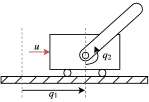
Figure 3a shows a simple example of a single rigid-body link. The simplest model that we can use for this system comes from Newton’s second law $u=J\ddot{q_{1}}$, where $u$ is the torque applied to the system, $J$ is the moment of inertia, and $q_{1}$ is the angle of the pendulum. Using Euler discretization method, we obtain the following state-space representation that serves as the prior $h({\boldsymbol{x}})^{T}{\boldsymbol{\beta}}$ for our EVGP model:

$$\begin{bmatrix}q_{1}[t+1]\\ \dot{q_{1}}[t+1]\end{bmatrix}= \begin{bmatrix}q_{1}[t]\\ \dot{q_{1}}[t]\end{bmatrix}+\Delta{t}\begin{bmatrix}\dot{q_{1}}[t]\\ \dfrac{1}{J}u[t]\end{bmatrix}$$ (6)

$$= \underbrace{\begin{bmatrix}1&\Delta{t}&0\\ 0&1&\Delta{t}/J\end{bmatrix}}_{{\boldsymbol{\beta}}\text{ prior mean }{{\boldsymbol{\mu}}_{\beta}}}\underbrace{\begin{bmatrix}q_{1}[t]\\ \dot{q_{1}}[t]\\ u[t]\end{bmatrix}}_{h({\boldsymbol{x}}_{[t]})}$$ (7)

We refer to this prior as IF (inertia+force). $\Delta{t}$ is the discretization time and $\begin{bmatrix}q_{1}[t]&\dot{q_{1}}[t]\end{bmatrix}^{T}$ is the state ${\boldsymbol{z}}_{[t]}$ of the system. The IF prior in Eq. 7 does not include gravitational effects. Gravity pulls the link to the downward position with a force proportional to $\sin{q_{1}}$. Hence, a prior that considers gravitational forces can be constructed by including $\sin(q_{1}[t])$:

$$\text{IFG}_{[t+1]}=\begin{bmatrix}1&\Delta{t}&0&0\\ 0&1&\Delta{t}/J&-\gamma\end{bmatrix}\begin{bmatrix}q_{1}[t]\\ \dot{q_{1}}[t]\\ u[t]\\ \sin(q_{1}[t])\end{bmatrix}$$ (8)

we call this prior IFG (inertia+force+gravity). We purposely did not define $J$ and $\gamma$. One of the advantages of the presented approach is that the algorithm can learn the parameters from data if they are not available. If the user does not know the value of $J$ and $\gamma$, a prior with large standard deviation can be provided for these parameters (large $\Sigma_{\boldsymbol{\beta}}$). Although parameters like $J$ and $\gamma$ are easy to compute for a simple pendulum, for more complex systems they may be hard and tedious to obtain. Our objective is to take advantage of domain knowledge and allow the model to fill in the gaps in knowledge.

For the rest of the paper, priors derived from Eq. 7 are referred as IF priors, while Eq. 8 priors are referred as IFG. In the experiments (section IV) we compare the performance for both priors in order to illustrate how performance can be progressively improved with more detailed priors.

(a) Pendulum

(b) Cartpole

(c) Acrobot

(d) IIWA (drake, )

Figure 3: Diagrams of physical systems considered

III-B Simplified priors for Acrobot, Cartpole and IIWA

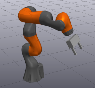
In addition to the pendulum, we consider the Acrobot, Cartpole, and IIWA systems in our analysis. For these systems, we consider much simpler priors than the exact dynamic models derived from multi-body dynamics. We use the same principles shown in the previous section in order to get simple priors for the systems. These rules are summarized as follows:

• The position should increase proportional to the velocity by a factor of $\Delta{t}$.

• The position should stay the same if the velocity is zero.

• The velocity should stay the same if no external forces are applied.

• For the IFG prior, gravity pulls the links to the downward position proportional to the sine of the angle w.r.t. the horizontal plane. Gravity has no effect when the links are completely down/up.

The objective with these priors is to demonstrate how extremely simplified priors extracted with simple physics can be used to improve performance of data-driven models. Figure 3c shows a diagram of the Acrobot system. A simple prior for this system can be constructed using the prior in Eq. 7 for each one of the links of the Acrobot:

IF $$=\begin{bmatrix}1&0&\Delta{t}&0&0\\ 0&1&0&\Delta{t}&0\\ 0&0&1&0&0\\ 0&0&0&1&\gamma_{1}\\ \end{bmatrix}\begin{bmatrix}q_{1}[t]\\ q_{2}[t]\\ \dot{q_{1}}[t]\\ \dot{q_{2}}[t]\\ u[t]\end{bmatrix}$$ (9)

IFG $$=\begin{bmatrix}1&0&\Delta{t}&0&0&0&0\\ 0&1&0&\Delta{t}&0&0&0\\ 0&0&1&0&0&-\gamma_{2}&-\gamma_{3}\\ 0&0&0&1&\gamma_{1}&0&-\gamma_{4}\\ \end{bmatrix}\begin{bmatrix}q_{1}[t]\\ q_{2}[t]\\ \dot{q_{1}}[t]\\ \dot{q_{2}}[t]\\ u[t]\\ \sin_{1}\\ \sin_{12}\end{bmatrix}$$ (10)

where $\sin_{1}=\sin(q_{1}[t])$, and $\sin_{12}=\sin(q_{1}[t]+q_{2}[t])$. In this case, the input $u[t]$ only drives the second link. The IF and IFG priors for the Cartpole (Figure 3b) are the following:

IF $$=\begin{bmatrix}1&0&\Delta{t}&0&0\\ 0&1&0&\Delta{t}&0\\ 0&0&1&0&\gamma_{1}\\ 0&0&0&1&0\\ \end{bmatrix}\begin{bmatrix}q_{1}[t]\\ q_{2}[t]\\ \dot{q_{1}}[t]\\ \dot{q_{2}}[t]\\ u[t]\end{bmatrix}$$

IFG $$=\begin{bmatrix}1&0&\Delta{t}&0&0&0\\ 0&1&0&\Delta{t}&0&0\\ 0&0&1&0&\gamma_{1}&0\\ 0&0&0&1&0&-\gamma_{2}\\ \end{bmatrix}\begin{bmatrix}q_{1}[t]\\ q_{2}[t]\\ \dot{q_{1}}[t]\\ \dot{q_{2}}[t]\\ u[t]\\ \sin(q_{2}[t])\end{bmatrix}$$

Figure 4: IFG prior for a Link in 3D

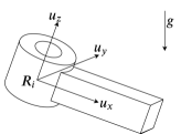
For the IIWA system, we constructed the priors following the same rules as before, with an approach that closely resembles to that used for the Acrobot. The priors were constructed using the prior in Eq. 7 for each one of the IIWA links. This results in a matrix ${\boldsymbol{\beta}}$ with a similar diagonal structure than the matrices in Eq. 10. To compute the IFG factors for $h()$, we derived an equation that can be used for a general 3D link (see Fig. 4). The equation uses forward kinematics to evaluate the contribution of the torque applied by gravity (${\boldsymbol{g}}$):

$$h^{i}_{IFG}\triangleq\left({\boldsymbol{u}}_{x}\times{\boldsymbol{R}}_{i}^{T}{\boldsymbol{g}}\right)\cdot{\boldsymbol{u}}_{z}$$

where $\times$ denotes cross product, $\cdot$ denotes dot product, and ${\boldsymbol{u}}_{x}$ and ${\boldsymbol{u}}_{z}$ are unit vectors. The matrix ${\boldsymbol{R}}_{i}$ is the rotation matrix of the frame attached to link $i$. This matrix is computed using classic forward kinematics, therefore its value depends on the value of ${\boldsymbol{q}}$. This equation basically computes the torque applied by gravity to the axis of rotation ${\boldsymbol{u}}_{z}$. We only use unitary vectors as we assume that information like the position of the center of gravity will be captured by the posterior of ${\boldsymbol{\beta}}$, i.e. the learned parameters.

These priors are extremely simple as they do not consider friction or coriolis/centrifugal forces. However, they provide important information about the mechanics of the system.

IV Experiments

In order to evaluate the performance of the presented model, we performed experiments on a set of simulated systems: Pendulum, Cartpole, Acrobot, and IIWA. We also performed qualitative tests on a toy-dataset to visualize the performance of the EVGP model.

We used Drake (drake, ) to simulate the Pendulum, Cartpole, Acrobot and IIWA systems and obtain the control/sensor data used to train and evaluate the EVGP models. We used the squared exponential function for the covariance kernels. The reason for this choice is that all the experiments involve continuous systems. The EVGP model was implemented using Tensorflow and the minimization of the negative ELBO loss was done using the ADAM optimizer (kingma2014adam, ). The experiments were run in a computer with a single GPU (Nvidia Quadro P5000) with an Intel(R) Xeon(R) CPU (E3-1505M at 3.00GHz).

IV-A Experiments on Toy Dataset

The toy dataset is intended to serve as an illustration of the behavior of the EVGP model and visualize the qualitative differences between several GP models. We use a modified version of the toy dataset used in (snelson2006sparse, ) (titsias2009variational, ). The dataset is modified as follows:

$$(y,x)\leftarrow(6y+3x,x)$$

The modification is intended to provide a global linear trend to the data (See Figure 5). Figure 5 shows the distribution learned using different versions of a Gaussian Process. Figures 5a and Figure 5c show the exact posterior distributions for a GP and EGP (rasmussen2004gaussian, ) model, respectively. Figures 5b and 5d show the variational approximations obtained with a VGP (hensman2013gaussian, ) and EVGP model. The standard deviation (black line) is used to visualize the uncertainty. The figures show how the uncertainty grows as we move away from the training dataset.

The original dataset is composed of 200 samples, Figure 5 shows that the variational approximations are able to successfully approximate their exact counterparts with as few inducing points as m=10. The position of the inducing points are shown with green crosses.

In this case, the prior-knowledge that we provide to the EVGP is a simple linear function $h(x,{\boldsymbol{\beta}})=x\beta_{1}+\beta_{2}$. Figure 5d shows how we can use the prior in order to control the global shape of the function. The figure shows how the EGP and EVGP models use the prior knowledge to fit the global behavior of the data (linear) while using the kernels to model the local non-linear behavior.

(a) GP regression

(b) VGP regression (m=10)

(c) EGP regression

(d) EVGP regression (m=10)

Figure 5: Regression on Toy Dataset. The presented EVGP model provides a tool for the user to control the global shape of the learned function without constraining the complexity. The GP kernels model local non-linear behavior that the global function $h({\boldsymbol{x}})$ is unable to model.

IV-B Learning system dynamics

We evaluated the performance of the EVGP model in learning system dynamics using data obtained from simulations of the Pendulum, Cartpole, Acrobot and IIWA systems. Concretely, we evaluated the accuracy of the EVGP model with IF and IFG priors in predicting the next state of the system given the current control inputs and state.

Data: to evaluate the difference in generalization, we sampled two different datasets for each system: one for training and one for testing. For the Pendulum, Cartpole, and Acrobot, the datasets were sampled by simulating the system using random initial states ${\boldsymbol{z}}_{[0]}\sim\alpha\;{{\cal U}\left(-1,1\right)}$ and random control inputs ${\boldsymbol{u}}_{[t]}\sim\eta\;{\cal N}\left(0,1\right)$ drawn from uniform and normal distributions, respectively. For the IIWA, the datasets were obtained by simulating the robot going from an initial position $\hat{{\boldsymbol{q}}}_{[0]}\sim{{\cal U}\left(-1.5,1.5\right)}$ to a final position $\hat{{\boldsymbol{q}}}_{[T]}\sim\hat{{\boldsymbol{q}}}_{[0]}+{{\cal U}\left(-0.8,0.8\right)}$. The IIWA was controlled by an inverse dynamics controller provided by the Drake library. We added normal noise with a scale of $0.1*[3,15,3,2,2,2,0.05]$ to the output of the controller. We had to use a controller for the IIWA in order to maintain the state of the robot inside a reasonable operating region. Table II shows the values of the scales ($\alpha,\eta$) that were used to sample the trajectories. These values were chosen in order to cover at least the range ($-\pi,\pi$) for the angles on the systems. In Table II, $H$ refers to the number of sampled trajectories, $\left\lvert{\cal D}\right\rvert$ refers to the total number of samples. All trajectories were sampled with $\Delta{t}=0.03s$.

TABLE I: Parameters used to collect training and testing data

System	$\alpha$	$\eta$	$H$	$\left\lvert{\cal D}\right\rvert$
Pendulum	[$\pi$, 0.5]	1.0	48	4800
Cartpole	[1.0, $\pi$, 0.5, 0.5]	100.0	48	4800
Acrobot	[$\pi$, 1.0, 0.5, 0.5]	0.5	93	9300
IIWA			465	23250

TABLE II: Number of inducing points and hidden units

	Pendulum	Cartpole	Acrobot	IIWA
VGP	40	100	250	500
RES-VGP	40	100	250	500
RES-DBNN	[15, 15]	[50, 50]	[60, 60]	[512, 512]
EVGP-IF	10	60	150	350
EVGP-IFG	10	60	150	350

Baseline: we compare the EVGP model with a standard VGP model hensman2013gaussian , a residual VGP (RES-VGP) deisenroth2011pilco hensman2013gaussian , and a residual Deep Bayesian Neural Network (RES-DBNN) kingma2015variational marino2019modeling . The VGP model is based on (hensman2013gaussian, ) and uses a zero mean prior. The residual VGP and DBNN models assume the system can be approximated as ${\boldsymbol{z}}_{[t+1]}={\boldsymbol{z}}_{[t]}+g_{r}({\boldsymbol{z}}_{[t]}\oplus{\boldsymbol{u}}_{[t]})$. Approximating residuals is a common approach used to simplify the work for GP and DBNN models (deisenroth2011pilco, ) (gal2016improving, ) (marino2019modeling, ). The RES-DBNN model is trained using the local reparameterization trick presented in (kingma2015variational, ) with Normal variational distributions for the weights. For these set of experiments, we did not consider the exact GP and EGP models given the large number of samples in the training datasets.

TABLE III: Complexity comparison

	Space	Time
VGP	$O(om)$	$O(om^{3})$
DBNN	$O(Ln^{2})$	$O(Ln^{2})$
EVGP	$O(om)$	$O(om^{3})$

Table II shows the number of inducing points (m) used for the VGP and EVGP models. The table also shows the number of hidden units for the DBNN model, where [15, 15] means a two-layer network with 15 units in each layer. We used the LeakyRelu activation function.

Table III shows the space and time complexity of the models considered in this paper. In this table, $m$ is the number of inducing points, $o$ is the number of outputs, $L$ is the number of hidden layers, and $n$ is the number of hidden units in each layer. To simplify the analysis, we assume all hidden layers of the DBNN have the same number of hidden units. The table shows that the complexity of the VGP and EVGP models are governed by the matrix inversion ${\boldsymbol{K}}_{mm}^{-1}$. Because we assume completely independent VGP and EVGP models for each output of the system, their complexity also depends on the number of outputs $o$. The complexity of the DBNN model is governed by the matrix-vector product between the weight matrices and the hidden activation vectors. All models have constant space complexity w.r.t. the training dataset size $\left\lvert{\cal D}\right\rvert$. Furthermore, all models have linear time complexity w.r.t. $\left\lvert{\cal D}\right\rvert$ if we assume that training requires to visit each sample in ${\cal D}$ at least once.

Metrics: for comparison, we used three metrics: 1) prediction error (Error), 2) predicted standard-deviation ($\|STD\|$), 3) containing ratios (CR). Prediction error is computed as the difference between sampled values ($y$) and the expected estimated output ($\mathop{{\mathbb{E}}}\left[\hat{y}^{(i)}\right]$). $\|\text{STD}\|$ is computed as the magnitude of the predicted standard deviation:

$$\text{Error}=\dfrac{1}{{\left\lvert{\cal D}\right\rvert}}\sum_{i=1}^{\left\lvert{\cal D}\right\rvert}\left\lVert y^{(i)}-\mathop{{\mathbb{E}}}\left[\hat{y}^{(i)}\right]\right\rVert$$ (11)

$$\|\text{STD}\|=\dfrac{1}{{\left\lvert{\cal D}\right\rvert}}\sum_{i=1}^{\left\lvert{\cal D}\right\rvert}\left\lVert{\text{STD}\left(\hat{y}^{(i)}\right)}\right\rVert$$ (12)

where ${\left\lvert{\cal D}\right\rvert}$ is the number of samples in the respective dataset. The expected output ($\mathop{{\mathbb{E}}}\left[\hat{y}^{(i)}\right]$) for the EVGP model is equal to $\mu_{\hat{{\boldsymbol{g}}}|\hat{{\boldsymbol{x}}}}$ in Eq. 4. For the DBNN model, the expectation is estimated using Monte-Carlo.

The containing ratios (CR) are the percentage of values covered by the estimated distribution $\hat{y}$. We consider containing ratios for one, two and three standard deviations (CR-1, CR-2, and CR-3 respectively). We expect the best model to have Error and $\|\text{STD}\|$ close to zero, while best containing ratios will be closer to the (68-95-99.7) rule of standard distributions.

Results: Table IV shows the prediction error and CR scores obtained in the testing dataset. EVGP-IF and EVGP-IFG refers to the use of an IF or IFG prior, respectively. We can observe a considerable improvement on the testing error and CR scores when using EVGP models. EVGP models provided the lowest error and best CR scores. We also see a progressive improvement on the testing error when using more detailed priors. The IFG prior provided lower prediction errors when compared with the IF prior. The EVGP-IFG model provided the estimations with the lowest prediction error, with low $\|STD\|$ and best CR scores. Table IV also shows that the EVGP model achieved the best performance using fewer number of parameters.

TABLE IV: Results on Testing Dataset

	Model	CR-1	CR-2	CR-3	Error	$\|STD\|$	# Param.
Pendulum	VGP	0.582	0.841	0.910	0.343	0.273	407
	RES-VGP	0.833	0.951	0.974	0.155	0.216	407
	RES-DBNN	0.691	0.908	0.959	0.017	0.010	634
	EVGP-IF	0.936	0.986	0.993	0.013	0.024	119
	EVGP-IFG	0.871	0.965	0.985	0.005	0.007	123
Cartpole	VGP	0.505	0.828	0.901	0.188	0.185	2813
	RES-VGP	0.518	0.848	0.924	0.216	0.153	2813
	RES-DBNN	0.336	0.767	0.901	0.044	0.036	6008
	EVGP-IF	0.933	0.980	0.990	0.016	0.184	1733
	EVGP-IFG	0.935	0.976	0.986	0.011	0.041	1741
Acrobot	VGP	0.715	0.861	0.913	1.100	2.137	7013
	RES-VGP	0.705	0.846	0.904	0.820	1.428	7013
	RES-DBNN	0.606	0.837	0.899	0.289	0.378	8408
	EVGP-IF	0.794	0.908	0.950	0.151	0.290	4253
	EVGP-IFG	0.712	0.893	0.952	0.131	0.251	4269
IIWA	VGP	0.000	0.051	0.311	0.048	0.039	161049
	RESVGP	0.002	0.163	0.519	0.055	0.047	161049
	DBNN	0.001	0.096	0.346	0.036	0.025	143028
	EVGP-IF	0.040	0.353	0.684	0.037	0.035	113337
	EVGP-IFG	0.083	0.480	0.773	0.027	0.030	113673

(a) Prediction error for all models

(b) Prediction error using IF and IFG priors

Figure 6: Prediction error on testing dataset for increasing number of training samples. The EVGP model provides the most accurate predictions while requiring less number of samples. Note that the number of training samples is in the order of thousands.

Figure 6 shows a comparison of the prediction error on the test dataset as we increase the number of training samples. For this experiment, we kept the testing dataset fixed while samples were progressively aggregated into the training dataset. The figure shows the mean, max and min values obtained for four independent runs. Figure 6a shows a comparison that includes all models. As expected, the prediction error is reduced as we increase the size of our training dataset. The figure shows that the EVGP provides the most accurate predictions while requiring less number of samples.

Figure 6a also shows how the performance of VGP and RES-VGP plateaus, struggling to take advantage of larger datasets. Although the RES-DBNN performs poorly with small training datasets, the high capacity of the RES-DBNN model allows it to take advantage or large datasets and improve accuracy, reducing the performance gap w.r.t. the EVGP models as more data is available. Thanks to the lower computational time-cost of the RES-DBNN (see Table III), this model can use a larger set of parameters without incurring in excessive training times.

Figure 6b shows a scaled version that only considers the EVGP model with different priors. This figure shows that the IFG prior provides more accurate predictions when compared to the IF prior. In the case of the pendulum, the IFG prior provides a highly accurate model of the system, requiring only a small number of training samples. Figure 6b also shows how as training data is aggregated, the accuracy gap between IF and IFG priors is reduced.

The priors that we use are extremely simple, they are ignoring friction and coriolis/centrifugal effects. Nonetheless, we observe a considerable performance improvement after providing our data-driven model basic information with the IF and IFG priors.

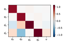
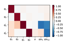
Understanding the learned model: one of the advantages of incorporating domain knowledge is that the learned model is easy to interpret by the domain expert. For example, in the case of the Acrobot, the value of the parameter ${\boldsymbol{\beta}}$ can be visualized to understand and debug what the model has learned. Figure 7 shows the value of ${\boldsymbol{b}}$ learned with the IF (Fig. 7a) and IFG priors (Fig. 7b).

We observe in Figure 7 that the learned parameters follow a similar structure given by the prior (see Eq. 10). In our experiments, we did not enforce the sparse structure from the priors, i.e. zero parameters in the prior are allowed to have non-zero values in the posterior.

Figure 7a shows that when using the IF prior, the EVGP model compensates for the missing gravity information by assigning negative values to $(\dot{q_{1}},q_{1})$ and $(\dot{q_{2}},q_{2})$. The reason for this behavior is that $q_{1}\approx\sin{q_{1}}$ for small $q_{1}$, however this approximation is no longer valid for large $q_{1}$. When using IFG priors (Fig. 7b), we observe that the model no longer assigns negative values to $(\dot{q_{1}},q_{1})$ and $(\dot{q_{2}},q_{2})$. The reason is that IFG provides the values of $sin(q_{1})$ and $sin(q_{1}+q_{2})$ which help to model the effect of gravity more accurately.

V Related work

Incorporating prior scientific knowledge in machine-learning algorithms is an ongoing effort that has recently gained increased attention. Hybrid modeling approaches that combine data and physics based methods are starting to gain attention in modeling cyber-physical systems (rai2019driven, ). Convolutional neural networks (CNNs) have been used in modeling and simulation applications such as forecasting of sea surface temperature (de2017deep, ) and efficient simulation of the Navier-Stokes equations (tompson2017accelerating, ). Hybrid models and physics-based loss functions have been introduced in physics-informed neural networks (raissi2019physics, ) (yang2019adversarial, ) in order to ensure that the trained neural network satisfies physics laws. In (bikmukhametov2020combining, ) first principles models are combined with machine learning to create deterministic models of process engineering systems. The machine learning model (LSTM or MLP) is trained separately to predict the mismatch between a first principles model and the target solution. No training is performed on the first principles model. The solutions of the first principles model and the machine learning model are added to provide the final prediction. Gaussian Processes (GP) have been used as a general purpose non-parametric model for system identification and control under uncertainty (deisenroth2011pilco, ) (bijl2017system, ). Previous work has explored using GPs to include partial model information (hall2012modelling, ). In (gray2018hybrid, ) the EGP model described in (rasmussen2004gaussian, ) is used in combination with a simplified physics model in a thermal building modelling application. Our work is based on the GP model with explicit features (EGP) presented in (rasmussen2004gaussian, ). Variations of this model are commonly used in calibration of computer models (kennedy2001bayesian, ) (li2016integrating, ). To the best of our knowledge, we are the first to apply variational inference to the EGP model in order to embed simplified physics models and improve scalability.

Despite the advantages of GP models for modeling complex non-linear relations with uncertainty, GPs are computationally expensive. A large bulk of research has focused on improving the computational requirements of GPs. Sparse GP approximation methods are some of the most common approaches for reducing GP computation cost (quinonero2005unifying, ). Bayesian approximation techniques such as Variational Inference provide a rich toolset for dealing with large quantities of data and highly complex models (kingma2013auto, ) (titsias2009variational, ). Variational approximations of a sparse GP have been explored in (titsias2009variational, ) (hensman2013gaussian, ). In (frigola2014variational, ) a variational GP model is presented for nonlinear state-space models. In (gal2016improving, ) (marino2019modeling, ), Deep Bayesian Neural Networks (DBNNs) are proposed as an alternative to GPs in order to improve scalability in reinforcement learning problems. Given the popularity of GP models and Variational Inference, there is an increased interest on developing automated variational techniques for these type of models (nguyen2014automated, ) (kucukelbir2017automatic, ).

(a) ${\boldsymbol{b}}$ using IF prior

(b) ${\boldsymbol{b}}$ using IFG prior

Figure 7: Visualization of the learned value of ${\boldsymbol{b}}$ for the Acrobot

VI Conclusion

In this paper, we presented the EVGP model, a stochastic data-driven model that is enhanced with domain knowledge extracted from simplified physics. The EVGP is a variational approximation of a Gaussian Process which uses domain knowledge to define the mean function of the prior. The priors provided a rough but simple approximation of the mechanics, informing the EVGP of important structure of the real system. We compared the performance of the EVGP model against purely data-driven approaches and demonstrated improved accuracy and interpretability after incorporating priors derived from simplified Newtonian mechanics. We showed that as we include more details into priors, the algorithm performance increases. We also showed how the difference between physics enhanced and purely data drive becomes smaller as we increase the availability of training data. We demonstrated that in case of smaller training data sets, the EVGP proved its superiority over the purely data driven approaches. Finally, we illustrate how visualizing the learned parameters can be useful to gain insights into the learned model and hence improve understandability.

Appendix A Variational Inference

In a Bayesian learning approach, we model the parameters $\omega$ of our model $p({\boldsymbol{y}}\mid{\boldsymbol{x}},\omega)$ using probability distributions. The parameters are given a prior distribution ${p\left(\omega\right)}$ that represents our prior knowledge about the model before looking at the data. Given a dataset ${\cal D}$, we would like to obtain the posterior distribution of our parameters following the Bayes rule:

$$p(\omega|{\cal D})=\frac{{p\left({\cal D}|\omega\right)}{p\left(\omega\right)}}{{p\left({\cal D}\right)}}$$

Variational Inference (VI) provides a tool for approximating the posterior $p(\omega|{\cal D})$ using a variational distribution ${p_{\phi}\left(\omega\right)}$ parameterized by $\phi$. In other words, with VI we find the value of $\phi$ such that ${p_{\phi}\left(\omega\right)}\approx p(\omega|{\cal D})$. The parameters $\phi$ of the distribution ${p_{\phi}\left(\omega\right)}$ are found by maximizing the Evidence Lower Bound (ELBO) between the approximate and real distributions:

$$\phi\leftarrow\operatorname*{arg\,max}_{\phi}\mathop{{\mathbb{E}}}_{{p_{\phi}\left(\omega\right)}}\left[\log{p\left({\cal D}\mid\omega\right)}\right]-D_{KL}\left({p_{\phi}\left(\omega\right)}\mid\mid{p\left(\omega\right)}\right)$$

Maximizing the ELBO is equivalent to minimizing the KL divergence between the variational distribution and the real distribution.

Having obtained the variational approximation ${p_{\phi}\left(\omega\right)}$, we can approximate the predictive distribution $p({\boldsymbol{y}}|{\boldsymbol{x}},{\cal D})$ as follows:

$$p({\boldsymbol{y}}|{\boldsymbol{x}},{\cal D})= \mathop{{\mathbb{E}}}_{p(\omega\mid{\cal D})}\left[p({\boldsymbol{y}}|{\boldsymbol{x}},\omega)\right]\approx\mathop{{\mathbb{E}}}_{{p_{\phi}\left(\omega\right)}}\left[p({\boldsymbol{y}}|{\boldsymbol{x}},\omega)\right]$$

which is the approximated variational predictive distribution ${p_{\phi}\left(\hat{{\boldsymbol{y}}}\mid\hat{{\boldsymbol{X}}}\right)}$ (see section II-C):

$${p_{\phi}\left(\hat{{\boldsymbol{y}}}\mid\hat{{\boldsymbol{X}}}\right)}=\mathop{{\mathbb{E}}}_{p_{\phi}(\omega)}\left[{p\left(\hat{{\boldsymbol{y}}}\mid\hat{{\boldsymbol{X}}},\omega\right)}\right]$$

Appendix B ELBO

Given the training dataset ${\cal D}=({\boldsymbol{y}},{\boldsymbol{X}})$, the parameters $\phi$ of ${p_{\phi}\left(\omega\right)}$ are learned by minimizing the negative Evidence Lower Bound (ELBO). For the EVGP, the negative ELBO takes the following form:

$${\mathcal{L}_{1}\left(\phi\right)}=-\mathop{{\mathbb{E}}}_{{p_{\phi}\left(\omega\right)}}\left[\ln\mathop{{\mathbb{E}}}_{g\mid\omega}\left[{p\left({\boldsymbol{y}}\mid{\boldsymbol{g}}\right)}\right]\right]+\mathcal{L}_{KL}$$ (B.1)

where $\mathcal{L}_{KL}$ denotes the KL divergence between the variational posterior and the prior $\mathcal{L}_{KL}=D_{KL}\left({p_{\phi}\left(\omega\right)}\mid\mid{p\left(\omega\right)}\right)$ Note that the inner expectation in Eq. B.1 is taken w.r.t. ${g\mid\omega}$, presented in Eq. 2. Following a similar approach than (hensman2013gaussian, ), we apply Jensen’s inequality in the inner expectation of Eq. B.1:

$$\log\mathop{{\mathbb{E}}}_{g\mid\omega}\left[{p\left({\boldsymbol{y}}\mid{\boldsymbol{g}}\right)}\right]\geq\mathop{{\mathbb{E}}}_{g\mid\omega}\left[\log{p\left({\boldsymbol{y}}\mid{\boldsymbol{g}}\right)}\right]$$

$$\mathop{{\mathbb{E}}}_{g\mid\omega}\left[\log{P\left({\boldsymbol{y}}\mid{\boldsymbol{g}}\right)}\right]=\log{\cal N}\left({\boldsymbol{y}}\mid{\boldsymbol{\mu}}_{{\boldsymbol{g}}\mid\omega},{\boldsymbol{\Sigma}}_{y}\right)-\dfrac{1}{2}\text{Tr}\left({\boldsymbol{\Sigma}}_{y}^{-1}{\boldsymbol{\Sigma}}_{{\boldsymbol{g}}\mid\omega}\right)$$

where ${\boldsymbol{\mu}}_{{\boldsymbol{g}}\mid\omega}={\boldsymbol{H}}_{x}{\boldsymbol{\beta}}+{\boldsymbol{\mu}}_{{\boldsymbol{f}}\mid\omega}$, ${\boldsymbol{\Sigma}}_{{\boldsymbol{g}}\mid\omega}={\boldsymbol{\Sigma}}_{{\boldsymbol{f}}\mid\omega}$. This allows us to express the ELBO in a way that simplifies the computation of the expectations w.r.t. the parameters $\omega$. Now, the variational loss in Eq. 3 can be obtained by simply computing the expectation w.r.t. the model parameters:

$${\mathcal{L}\left(\phi\right)}= \mathop{{\mathbb{E}}}_{{p_{\phi}\left(\omega\right)}}\left[\mathop{{\mathbb{E}}}_{g\mid\omega}\left[-\log{p\left({\boldsymbol{y}}\mid{\boldsymbol{g}}\right)}\right]\right]+\mathcal{L}_{KL}$$

$$= -\mathop{{\mathbb{E}}}_{{p_{\phi}\left(\omega\right)}}\left[\log{\cal N}\left({\boldsymbol{y}}\mid{\boldsymbol{\mu}}_{{\boldsymbol{g}}\mid\omega},{\boldsymbol{\Sigma}}_{y}\right)-\dfrac{1}{2}\text{Tr}\left({\boldsymbol{\Sigma}}_{y}^{-1}{\boldsymbol{\Sigma}}_{{\boldsymbol{g}}\mid\omega}\right)\right]$$

$$+\mathcal{L}_{KL}$$

$$= -\log{\cal N}\left({\boldsymbol{y}}\mid{\boldsymbol{H}}_{x}{\boldsymbol{b}}+{\boldsymbol{K}}_{xm}{\boldsymbol{K}}_{mm}^{-1}{\boldsymbol{a}},{\boldsymbol{\Sigma}}_{y}\right)$$

$$+\dfrac{1}{2}\left[\text{Tr}\left({\boldsymbol{M}}_{1}{\boldsymbol{A}}\right)+\text{Tr}\left({\boldsymbol{M}}_{2}{\boldsymbol{B}}\right)+\text{Tr}\left({\boldsymbol{\Sigma}}_{y}^{-1}{\boldsymbol{\Sigma}}_{{\boldsymbol{f}}\mid\omega}\right)\right]$$

$$+\mathcal{L}_{KL}$$

where ${\boldsymbol{M}}_{1}=\left({\boldsymbol{K}}_{mm}^{-1}{\boldsymbol{K}}_{mx}\right){\boldsymbol{\Sigma}}_{y}^{-1}\left({\boldsymbol{K}}_{xm}{\boldsymbol{K}}_{mm}^{-1}\right)$, and ${\boldsymbol{M}}_{2}={\boldsymbol{H}}_{x}^{T}{\boldsymbol{\Sigma}}_{y}^{-1}{\boldsymbol{H}}_{x}$. The value of the KL-divergence is simply the sum of the divergence for both parameters:

$$\mathcal{L}_{KL}= D_{KL}\left({\cal N}\left({\boldsymbol{a}},{\boldsymbol{A}}\right)\mid\mid{\cal N}\left(0,{\boldsymbol{K}}_{mm}\right)\right)$$

$$+D_{KL}\left({\cal N}\left({\boldsymbol{b}},{\boldsymbol{B}}\right)\mid\mid{\cal N}\left({\boldsymbol{\mu}}_{\beta},{\boldsymbol{\Sigma}}_{\beta}\right)\right)$$

Appendix C Mini-batch optimization

In order to make the model scalable to very large datasets, the ELBO can be optimized using mini-batches. Following (gal2016dropout, ), assuming the samples are i.i.d., the loss for a mini-batch $({\boldsymbol{y}},{\boldsymbol{X}})$ composed of $\left\lvert{\boldsymbol{X}}\right\rvert$ number of samples can be expressed as follows:

$${\mathcal{L}\left(\phi\right)}=-\dfrac{1}{\left\lvert{\boldsymbol{X}}\right\rvert}\mathop{{\mathbb{E}}}_{p_{\phi}(w)}\left[{\ln\left(p({\boldsymbol{Y}}|{\boldsymbol{X}},w)\right)}\right]+\dfrac{1}{\left\lvert{\cal D}\right\rvert}\mathcal{L}_{KL}$$

where $\left\lvert{\cal D}\right\rvert$ is the total number of samples in the training dataset.

Daniel L. Marino (marinodl@vcu.edu) received his B.Eng. in automation engineering from La Salle University, Colombia, in 2015. He is currently a research assistant and a doctoral student at Virginia Commonwealth University. His research interests include stochastic modeling, deep learning and optimal control.

Milos Manic (misko@ieee.org) (SM’06-M’04-StM’96) received the Dipl.Ing. and M.S. degrees in electrical engineering and computer science from the University of Niš, Niš, Serbia in 1991 and 1997 respectively, and the Ph.D. degree in computer science from the University of Idaho in 2003. Dr. Manic is a Professor with Computer Science Department and Director of VCU Cybersecurity Center at Virginia Commonwealth University. He completed over 30 research efforts in the area of data mining and machine learning applied to cybersecurity, critical infrastructure protection, energy security, and resilient intelligent control. Dr. Manic has given over 30 invited talks around the world, authored over 180 refereed articles in international journals, books, and conferences, holds several U.S. patents and has won 2018 R&D 100 Award for Autonomic Intelligent Cyber Sensor (AICS). He is an officer of IEEE Industrial Electronics Society, founding chair of IEEE IES Technical Committee on Resilience and Security in Industry, and general chair of IEEE IECON 2018, IEEE HSI 2019.

References

- (1) C. Szegedy, W. Liu, Y. Jia, P. Sermanet, S. Reed, D. Anguelov, D. Erhan, V. Vanhoucke, and A. Rabinovich, “Going deeper with convolutions,” in Proceedings of the IEEE conference on computer vision and pattern recognition, pp. 1–9, 2015.
- (2) A. Adadi and M. Berrada, “Peeking inside the black-box: A survey on explainable artificial intelligence (xai),” IEEE Access, vol. 6, pp. 52 138–52 160, 2018.
- (3) R. Frigola, Y. Chen, and C. E. Rasmussen, “Variational gaussian process state-space models,” in Advances in Neural Information Processing Systems, pp. 3680–3688, 2014.
- (4) D. Marino, K. Amarasinghe, M. Anderson, N. Yancey, Q. Nguyen, K. Kenney, and M. Manic, “Data driven decision support for reliable biomass feedstock preprocessing,” in Resilience Week (RWS), 2017, pp. 97–102. IEEE, 2017.
- (5) C. E. Rasmussen, “Gaussian processes in machine learning,” in Advanced lectures on machine learning, pp. 27–29. Springer, 2004.
- (6) J. Quiñonero-Candela and C. E. Rasmussen, “A unifying view of sparse approximate gaussian process regression,” Journal of Machine Learning Research, vol. 6, no. Dec, pp. 1939–1959, 2005.
- (7) M. Titsias, “Variational learning of inducing variables in sparse gaussian processes,” in Artificial Intelligence and Statistics, pp. 567–574, 2009.
- (8) R. Tedrake and the Drake Development Team, “Drake: A planning, control, and analysis toolbox for nonlinear dynamical systems,” 2016. [Online]. Available: https://drake.mit.edu
- (9) D. P. Kingma and J. Ba, “Adam: A method for stochastic optimization,” arXiv preprint arXiv:1412.6980, 2014.
- (10) E. Snelson and Z. Ghahramani, “Sparse gaussian processes using pseudo-inputs,” in Advances in neural information processing systems, pp. 1257–1264, 2006.
- (11) J. Hensman, N. Fusi, and N. D. Lawrence, “Gaussian processes for big data,” arXiv preprint arXiv:1309.6835, 2013.
- (12) M. Deisenroth and C. E. Rasmussen, “Pilco: A model-based and data-efficient approach to policy search,” in Proceedings of the 28th International Conference on machine learning (ICML-11), pp. 465–472, 2011.
- (13) D. P. Kingma, T. Salimans, and M. Welling, “Variational dropout and the local reparameterization trick,” in Advances in Neural Information Processing Systems, pp. 2575–2583, 2015.
- (14) D. Marino and M. Manic, “Modeling and planning under uncertainty using deep neural networks,” IEEE Transactions on Industrial Informatics, DOI 10.1109/TII.2019.2917520, pp. 1–1, 2019.
- (15) Y. Gal, R. T. McAllister, and C. E. Rasmussen, “Improving pilco with bayesian neural network dynamics models,” in Data-Efficient Machine Learning workshop, 2016.
- (16) R. Rai and C. K. Sahu, “Driven by data or derived through physics? a review of hybrid physics guided machine learning techniques with cyber-physical system (cps) focus,” IEEE Access, pp. 1–1, 2020.
- (17) E. de Bezenac, A. Pajot, and P. Gallinari, “Deep learning for physical processes: Incorporating prior scientific knowledge,” arXiv preprint arXiv:1711.07970, 2017.
- (18) J. Tompson, K. Schlachter, P. Sprechmann, and K. Perlin, “Accelerating eulerian fluid simulation with convolutional networks,” in Proceedings of the 34th International Conference on Machine Learning-Volume 70, pp. 3424–3433. JMLR. org, 2017.
- (19) M. Raissi, P. Perdikaris, and G. E. Karniadakis, “Physics-informed neural networks: A deep learning framework for solving forward and inverse problems involving nonlinear partial differential equations,” Journal of Computational Physics, vol. 378, pp. 686–707, 2019.
- (20) Y. Yang and P. Perdikaris, “Adversarial uncertainty quantification in physics-informed neural networks,” Journal of Computational Physics, vol. 394, pp. 136–152, 2019.
- (21) T. Bikmukhametov and J. Jäschke, “Combining machine learning and process engineering physics towards enhanced accuracy and explainability of data-driven models,” Computers & Chemical Engineering, p. 106834, 2020.
- (22) H. Bijl, T. B. Schön, J.-W. van Wingerden, and M. Verhaegen, “System identification through online sparse gaussian process regression with input noise,” IFAC Journal of Systems and Control, vol. 2, pp. 1–11, 2017.
- (23) J. Hall, C. Rasmussen, and J. Maciejowski, “Modelling and control of nonlinear systems using gaussian processes with partial model information,” in 2012 IEEE 51st IEEE Conference on Decision and Control (CDC), pp. 5266–5271. IEEE, 2012.
- (24) F. M. Gray and M. Schmidt, “A hybrid approach to thermal building modelling using a combination of gaussian processes and grey-box models,” Energy and Buildings, vol. 165, pp. 56–63, 2018.
- (25) M. C. Kennedy and A. O’Hagan, “Bayesian calibration of computer models,” Journal of the Royal Statistical Society: Series B (Statistical Methodology), vol. 63, no. 3, pp. 425–464, 2001.
- (26) W. Li, S. Chen, Z. Jiang, D. W. Apley, Z. Lu, and W. Chen, “Integrating bayesian calibration, bias correction, and machine learning for the 2014 sandia verification and validation challenge problem,” Journal of Verification, Validation and Uncertainty Quantification, vol. 1, no. 1, p. 011004, 2016.
- (27) D. P. Kingma and M. Welling, “Auto-encoding variational bayes,” arXiv preprint arXiv:1312.6114, 2013.
- (28) T. V. Nguyen and E. V. Bonilla, “Automated variational inference for gaussian process models,” in Advances in Neural Information Processing Systems, pp. 1404–1412, 2014.
- (29) A. Kucukelbir, D. Tran, R. Ranganath, A. Gelman, and D. M. Blei, “Automatic differentiation variational inference,” The Journal of Machine Learning Research, vol. 18, no. 1, pp. 430–474, 2017.
- (30) Y. Gal and Z. Ghahramani, “Dropout as a bayesian approximation: Representing model uncertainty in deep learning,” in international conference on machine learning, pp. 1050–1059, 2016.
![[Uncaptioned image]](/html/1906.02160/assets/x9.png) |