On hilltop and brane inflation after Planck

Abstract

Hilltop inflation models are often described by potentials $V=V_{0}(1-{\phi^{n}\over m^{{n}}}+...)$. The omitted terms indicated by ellipsis do not affect inflation for $m\lesssim 1$, but the most popular models with $n=2$ and $4$ for $m\lesssim 1$ are ruled out observationally. Meanwhile in the large $m$ limit the results of the calculations of the tensor to scalar ratio $r$ in the models with $V=V_{0}(1-{\phi^{n}\over m^{{n}}})$, for all $n$, converge to $r=4/N\lesssim 0.07$, as in chaotic inflation with $V\sim\phi$, suggesting a reasonably good fit to the Planck data. We show, however, that this is an artifact related to the inconsistency of the model $V=V_{0}(1-{\phi^{n}\over m^{{n}}})$ at $\phi>m$. Consistent generalizations of this model in the large $m$ limit typically lead to a much greater value $r=8/N$, which negatively affects the observational status of hilltop inflation. Similar results are valid for D-brane inflation with $V=V_{0}(1-{m^{n}\over\phi^{{n}}})$, but consistent generalizations of D-brane inflation models may successfully complement $\alpha$-attractors in describing most of the area in the ($n_{s}$, $r$) space favored by Planck 2018.

1 Introduction

The Planck 2018 data release Akrami:2018odb provides a detailed review of a large family of inflationary models in comparison with observational data. Some of the most important results are described in Sect. 4.2 of Akrami:2018odb , especially in the Table 5, and also in the Fig. 8, which we reproduce below.

Figure 1: Inflationary models and the Planck 2018 results, according to Akrami:2018odb .

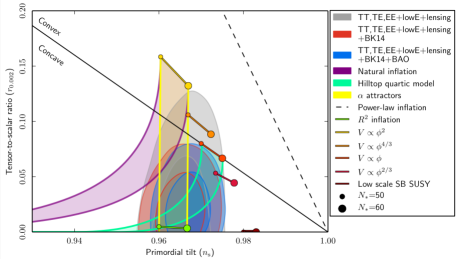
The models providing the best fit to the observational data include various versions of $\alpha$-attractors shown at Fig. 1 by a vertical yellow stripe, as well as the Starobinsky model and the Higgs inflation model shown by the small green disks at the lower end of the yellow $\alpha$-attractor stripe. Another set of models matching the Planck data are the hilltop models with the potentials $V=V_{0}(1-{\phi^{n}\over m^{{n}}}+...)$ and the so-called D-brane inflation models with the potentials $V=V_{0}(1-{m^{n}\over\phi^{{n}}}+...)$ for $n=2$ and $n=4$, see Table 5 in Akrami:2018odb . In the Planck 2013 and 2015 data releases Planck:2013jfk ; Ade:2015lrj it was emphasized that the omitted higher order terms shown by ellipsis are supposed to stabilize the potential from below. Moreover, it was pointed out in Ade:2015lrj that consistent modifications of the hilltop model with $n=2$, such as the simplest Higgs model $V=V_{0}(1-{\phi^{2}\over m^{{2}}})^{2}$, do not fit the data too well. The subsequent numerical analysis was performed for the models $V=V_{0}(1-{\phi^{n}\over m^{{n}}})$, with emphasis on $n=4$. The results for $n=4$ are shown by the green area in Fig. 1. Similarly, the analysis of D-brane inflation was performed for $V=V_{0}(1-{m^{n}\over\phi^{{n}}})$, see Table 5 in Akrami:2018odb .

These results play important role not only in evaluation of the presently available inflationary models, but also in the planning of the new generations of the cosmological observations. In particular, Fig. 10 in the CMB-S4 Science Book Abazajian:2016yjj , Fig. 1 of the CMB-S4 Science Case Abazajian:2019eic , and Fig. 2.2 in the PICO report Hanany:2019lle illustrate the present status of inflationary models related to their plans by the vertical stripe describing $\alpha$-attractors, as well as the green area corresponding to the hilltop models with the potentials $V=V_{0}(1-{\phi^{4}\over m^{{4}}})$. That is why we decided to revisit these three classes of models favored by the Planck data. Since we extensively studied $\alpha$-attractors in many other papers, we will only briefly review them in this paper, and concentrate on the hilltop and D-brane inflation models.

A large family of cosmological attractors, including the $\alpha$-attractors, was discovered shortly after the Planck 2013 data release Kallosh:2013hoa ; Kallosh:2013tua ; Ferrara:2013rsa ; Kallosh:2013yoa ; Kallosh:2014rga ; Kallosh:2014laa ; Galante:2014ifa . It was a result of our attempts to understand the mysterious nearly exact coincidence of the cosmological predictions of the Starobinsky model Starobinsky:1980te and the Higgs inflation model Salopek:1988qh ; Bezrukov:2007ep . We found that the main reason of this coincidence is that at the intermediate steps of the transformation from the original formulation of these models to the Einstein frame one encounters a scalar field with a kinetic term having a quadratic pole at a certain value of the field. This singularity disappears after transition to canonical variables.

A similar pole appears also in the model of conformal attractors Kallosh:2013hoa , which lead to the same predictions $n_{s}=1-2/N$ and $r=12/N$ as the Starobinsky model and the Higgs inflation model. Here $N$ is the number of e-foldings. An advantage of conformal attractors is that these predictions are practically independent on the choice of the original potential, which is why we called these models “attractors”. This property is shared by the generalization of the Higgs inflation proposed in Kallosh:2013tua . Finally, a more general family of cosmological attractors was found, called $\alpha$-attractors Ferrara:2013rsa ; Kallosh:2013yoa ; Kallosh:2014rga ; Kallosh:2014laa ; Galante:2014ifa . In the supergravity generalizations of this model, the pole appears as a result of the underlying hyperbolic geometry of the moduli space Carrasco:2015uma . In these models one has

$$n_{s}=1-{2\over N},\qquad r={12\alpha\over N}\ ,$$ (1)

which coincides with the predictions of the Starobinsky model, Higgs inflation and conformal attractors for $\alpha=1$, and with the predictions of the GL model Goncharov:1985yu ; Linde:2014hfa for $\alpha=1/9$. The $\phi^{2}$ potential corresponds to the limit of infinite $\alpha$ and this parameter decreases with decreasing $r$. With $N$ in the interval from $50$ to $60$, these predictions span the range shown by the yellow area in Fig. 1.

In this paper we will briefly describe $\alpha$-attractors, and then turn our attention to hilltop inflation models with $V=V_{0}(1-{\phi^{n}\over m^{{n}}}+...)$ Linde:1981mu ; Kinney:1995cc ; Boubekeur:2005zm and D-brane inflation with $V=V_{0}(1-{m^{n}\over\phi^{{n}}}+...)$ Dvali:2001fw ; Burgess:2001fx ; GarciaBellido:2001ky ; Kachru:2003sx ; Martin:2013tda ; Kallosh:2018zsi . In the limit $m\ll 1$, the predictions of both models are fairly stable with respect to the unspecified higher order terms shown by ellipsis in these equations. The most interesting versions of both models correspond to $n=4$. The hilltop inflation with $n=4$ in the limit $m\ll 1$ describes an attractor with

$$n_{s}=1-{3\over N},\qquad r={8m^{4}\over N^{3}}\ .$$ (2)

For $N=50$ one has $n_{s}=0.94$, and for $N=60$ one has $n_{s}=0.95$. Both results strongly disagree with observational data.

However, if one considers an opposite limit $m\gg 1$ and ignores the ellipsis, reducing the theory to $V=V_{0}(1-{\phi^{n}\over m^{{n}}})$, then one finds that in the large $m$ limit the predictions of this theory converge to the predictions of inflation with a linear potential $V\sim\phi$,

$$n_{s}=1-{3\over 2N},\qquad r={4\over N}\ .$$ (3)

The green area in Fig. 1 describing this theory interpolates between the two attractor points (2) and (3). Both attractor points are bad: $n_{s}=1-{3\over N}$ in (2) is too small, and $r=4/N$ in (3) is too large, but on its way between these two attractors, the green area significantly overlaps with the area favored by Planck 2018.

The situation becomes even more interesting if one takes into account that in the large $m$ limit the predictions of the model with a linear potential (3) is an attractor point for the hilltop inflation with $V=V_{0}(1-{\phi^{n}\over m^{{n}}})$ not only for $n=4$, but for any $n$, and not only for the hilltop inflation, but also for the D-brane inflation with $V=V_{0}(1-{m^{n}\over\phi^{{n}}})$ Martin:2013tda .

One may wonder why such a large class of different rather complicated models leads to the same prediction as the simplest model with the linear potential? Could it be that by revealing the deep physical reason of this remarkable result one can learn something important, just as we did when we tried to understand the nearly exact coincidence of the results of the Starobinsky and the Higgs inflation model?

Unfortunately, as we will see, this mysterious result is not so mysterious after all. The common feature of hilltop models $V=V_{0}(1-{\phi^{n}\over m^{{n}}})$ and D-brane inflation models $V=V_{0}(1-{m^{n}\over\phi^{{n}}})$ is that in the large $m$ limit the last 60 e-foldings of inflation in these models occur when the field $\phi$ moves from $\phi\sim m-10$ to $m-1/\sqrt{2}$ (from $\phi\sim m+10$ to $m+1/\sqrt{2}$ for the D-brane models). For $m\gg 10$ and $\phi>0$, these potentials look like a straight line $V\propto m-\phi$ ($V\propto\phi-m$ for D-brane models), which explains why all of these potentials have the same prediction (3) in the large $m$ limit.

But this means that the remarkable coincidence discussed above is directly related to the fact that the end of inflation in these models occurs shortly before the inflaton field hits the point $\phi=m$ with $V(\phi)=0$, falls towards $V(\phi)<0$, and the whole universe collapses. Thus such models are not good.

The models with the potentials unbounded from below are bad for any $m$. Therefore in the description of these models in the Planck 2013 data release it was emphasized that the higher order terms should stabilize the vacuum. For $m\lesssim 1$, one can easily add terms higher order in ${\phi\over m}$, forming a minimum of the potential at $V\geq 0$, without altering inflationary predictions of the original model. But the most natural attempts to improve these models at $m\gg 1$ significantly change their predictions. If we want to stick to the original design, considering the potentials $V({\phi\over m})$, then in the large $m$ limit the modified hilltop potentials near their minima in the first approximation are not linear but quadratic, on scale $\Delta\phi\equiv|m-\phi|\gg 1$. This is a rather general result described in Kallosh:2014rga ; Kallosh:2014laa in a different context. Therefore in the large $m$ limit the predictions of these models converge to the predictions of the chaotic inflation potential $V\sim\phi^{2}$, which yields

$$n_{s}=1-{2\over N},\qquad r={8\over N}\ .$$ (4)

In application to consistent versions of the quadratic hilltop models $V=V_{0}(1-{\phi^{2}\over m^{{2}}})$, such as the Higgs potential $V=V_{0}(1-{\phi^{2}\over m^{{2}}})^{2}$, this result was already discussed in the Planck 2015 data release Ade:2015lrj , but we found that it is valid for any $n$, including $n=4$. Thus the improved versions of the hilltop models in the large $m$ limit typically predict $r={8\over N}$, which is twice as large as the naive prediction $r={4\over N}$ of the hilltop models with the potentials $V=V_{0}(1-{\phi^{n}\over m^{{n}}})$.

A similar problem affects the D-brane inflation models $V=V_{0}(1-{m^{n}\over\phi^{{n}}})$, where the improved versions of these models typically lead to a much greater value of $r$ in the large $m$ limit. Now that we are aware of this problem, we will take a second look at all of these models, starting with $\alpha$-attractors, and then discuss hilltop and D-brane models in detail, going one step beyond the simplest versions of these theories.

2 $\alpha$-attractors

The basic principles of the theory of $\alpha$-attractors can be explained using a simple toy model with the Lagrangian Galante:2014ifa ; Kallosh:2015zsa

$${1\over\sqrt{-g}}\mathcal{L}={R\over 2}-{(\partial_{\mu}\phi)^{2}\over 2(1-{\phi^{2}\over 6\alpha})^{2}}-V(\phi)\,.$$ (5)

Here $\phi(x)$ is the scalar field, the inflaton. The origin of the pole in the kinetic term can be explained in the context of hyperbolic geometry in supergravity and string theory. The parameter $\alpha$ can take any positive value. Instead of the variable $\phi$, one can use a canonically normalized field $\varphi$ by solving the equation ${\partial\phi\over 1-{\phi^{2}\over 6\alpha}}=\partial\varphi$, which yields $\phi=\sqrt{6\alpha}\,\tanh{\varphi\over\sqrt{6\alpha}}$. The full theory, in terms of the canonical variables, becomes

$${1\over\sqrt{-g}}\mathcal{L}={R\over 2}-{(\partial_{\mu}\varphi)^{2}\over 2}-V\big{(}\sqrt{6\alpha}\,\tanh{\varphi\over\sqrt{6\alpha}}\big{)}\,.$$ (6)

If the potential and its derivatives are non-singular at $\phi=\sqrt{6\alpha}$, the asymptotic behavior of the potential at large $\varphi>0$ is given by

$$V(\varphi)=V_{0}-2\sqrt{6\alpha}\,V^{\prime}_{0}\ e^{-\sqrt{2\over 3\alpha}\varphi}\ .$$ (7)

Here $V_{0}=V(\phi)|_{\phi=\sqrt{6\alpha}}$ is the height of the plateau potential, and $V^{\prime}_{0}=\partial_{\phi}V|_{\phi=\sqrt{6\alpha}}$. Importantly, the coefficient $2\sqrt{6\alpha}\,V^{\prime}_{0}$ in front of the exponent can be absorbed into a redefinition (shift) of the field $\varphi$. Therefore all inflationary predictions of this theory in the regime with $e^{-\sqrt{2\over 3\alpha}\varphi}\ll 1$ are determined only by two parameters, $V_{0}$ and $\alpha$.

The amplitude of inflationary perturbations $A_{s}$ in these models matches the Planck normalization for ${V_{0}\over\alpha}\sim 10^{{-10}}$. For the simplest model $V={m^{2}\over 2}\phi^{2}$, belonging to a class of T-models with the potential symmetric with respect to $\phi\to-\phi$, one finds

$$V=3m^{2}\alpha\tanh^{2}{\varphi\over\sqrt{6\alpha}}\ .$$ (8)

Then the condition ${V_{0}\over\alpha}\sim 10^{{-10}}$ reads $m\sim 0.6\times 10^{{-5}}$. The cosmological predictions of this model are shown by the yellow vertical stripe in Fig. 1.

We should note that even though the predictions for large $N$ and small $\alpha$ are rather well defined, the value of $N$ itself does depend on the mechanism of reheating and post-inflationary equation of state, which is reflected in the uncertainty of the choice between $N\sim 50$ and $N\sim 60$. Also, predictions of different versions of $\alpha$-attractors converge to their target (1) in a slightly different way. For example, one may start with a model

$${1\over\sqrt{-g}}\mathcal{L}={R\over 2}-{3\alpha\over 4}\left({\partial_{\mu}t\over t}\right)^{2}-V(t)\,.$$ (9)

One can represent this model in terms of canonical variables $\varphi$, where $t=e^{-\sqrt{2\over 3\alpha}\varphi}$. For $V=V_{0}(1-t)^{2}$ this leads to a class of E-models with

$$V(\varphi)=V_{0}\left(1-e^{-\sqrt{2\over 3\alpha}\varphi}\right)^{2},$$ (10)

which coincides with the potential in the Starobinsky model for $\alpha=1$. The difference between this model for $\alpha=1$ and the original Starobinsky model Starobinsky:1980te is that adding extra terms $R^{n}$ to the Starobinsky model Starobinsky:1980te can easily affect the plateau shape of its potential, whereas the asymptotic plateau shape of the $\alpha$-attractor potential (10) at large $\varphi$ is quite stable with respect to considerable modifications of the original potential $V(t)$, and, as a consequence, stable with respect to quantum corrections Kallosh:2016gqp .

Figure 2: Red lines show predictions of the simplest E-models (10) for $N=50$ and $N=60$. These lines go very close to the yellow lines corresponding to the simplest T-model (8). These two basic $\alpha$-attractor models together cover a significant part of the area favored by Planck 2018.

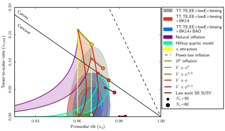
Note that the predictions of the E-models (10) coincide with the predictions of the T-models (8) in the limit $\alpha\to 0$ and $\alpha\to\infty$. In the intermediate range of $\alpha$, the simplest E-models (10) predict slightly larger values of $n_{s}$ than the simplest T-models (8). These two models together cover a significant part of the area in the $n_{s},r$ space favored by Planck 2018, see Fig. 2.

The predictions of these two classes of models nearly coincide with the predictions of the Starobinsky model and Higgs inflation model for $\alpha=1$, but $\alpha$-attractors allow much greater flexibility with respect to the tensor to scalar ratio $r$. In this respect, $\alpha$-attractors are more “future-safe”, allowing to describe and parametrize various outcomes of the B-mode searches.

3 Hilltop inflation after Planck 2018

Hilltop inflation may seem to provide a similarly good fit to the Planck data. The green band representing it is prominently shown in Fig. 8 of the Planck 2018 paper on inflation, which we reproduced in Fig. 1 of our paper. It is also shown in Fig. 10 of the CMB-S4 Science Book Abazajian:2016yjj and in Fig. 2.2 in PICO paper Hanany:2019lle .

The first example of hilltop inflation models was given by the Coleman-Weinberg potential used in the new inflation scenario Linde:1981mu

$$V={V_{0}}\,\left(1+{\phi^{4}\over m^{4}}\bigl{(}2\log{\phi^{2}\over m^{2}}-1\bigr{)}\right)\ .$$ (11)

Later on, it became customary to consider hilltop potentials of a more general type,

$$V=V_{0}\,\left(1-{\phi^{n}\over m^{n}}+...\right)\ ,$$ (12)

where the extra terms indicated by … are supposed to be responsible for creating a minimum of the potential Kinney:1995cc ; Boubekeur:2005zm . The simplest possibility is that such terms are higher order in $\phi^{n}\over m^{n}$. For $n=4$, this potential well represents the behavior of the Coleman-Weinberg potential near the top of the potential. One can show that for the small field models with $m\ll 1$, inflation occurs at $\phi\ll m$, where the higher order terms are negligible, and therefore some uncertainty in the definition of the potential at $\phi\sim m$ does not affect inflationary predictions.

That is why the calculation of $n_{s}$ and $r$ in many papers on this issue, including the Planck 2018 paper on inflation Akrami:2018odb , is performed for the simplest models

$$V=V_{0}\,\left(1-{\phi^{n}\over m^{n}}\right)\ ,$$ (13)

ignoring the terms indicated by $...$. However, for $m\lesssim 1$, the most popular hilltop models with $n=4$ shown in Fig. 1 predict $n_{s}=0.94$ for $N=50$ and $n_{s}=0.95$ for $N=60$. Such models are ruled out by observational data.

These predictions change for $m\gtrsim 1$, but they approach safer values $n_{s}\gtrsim 0.96$ favored by Planck 2018 only for $m\gtrsim 10$. In the large $m$ limit the green lines describing predictions of this model in Fig. 1 converge at the red circles corresponding to the predictions of inflation in the theory with a linear potential $V\sim\phi$. Moreover, a similar result is correct not only for $n=4$, but for all hilltop potentials (13) Martin:2013tda . How can the complicated theories (13) in the large $m$ limit give the same prediction as the theory with a simple potential $V\sim\phi$? What is going on?

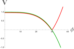
To answer this question, let us look at the the potential (13), which is shown by the green line in Fig. 3. This potential has a maximum (hilltop) at $\phi=0$, and then $V(\phi)$ decreases and becomes zero at $\phi=m$. Because the potential does not have any minimum at $\phi\sim m$, the potential at $\phi\approx m$ can be well approximated by a straight line. This approximation becomes better and better at large $m$, since the increase of $m$ stretches the potential horizontally. For $m\gg 10$, the last 50 e-foldings in this scenario are effectively described by a linear potential proportional to $m-\phi$. In this sense, the name “hilltop inflation” becomes a misnomer. The last 50 e-foldings in this scenario occur when the field moves down from $\phi\approx m-10$. The slow-roll parameter $\epsilon$ in this effective theory is given by ${1\over 2(m-\phi)^{2}}$, it is smaller than 1 and inflation continues until the point $m-\phi_{\rm end}\approx 1/\sqrt{2}$. Investigation of inflation in this scenario could suggest that its predictions provide a good match to Planck data. But this conclusion would be premature because such models suffer from the graceful exit problem.

Figure 3: Three hilltop potentials for $V_{0}=1$ with $m=50$. The hilltop potential (13) unbounded from below is shown by the green line. The Coleman-Weinberg potential (11) is shown by the blue line, and the quartic Higgs-type version of the hilltop potential (14) is shown by the red line.

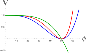
Indeed, after the end of inflation at $m-\phi_{\rm end}\approx 1/\sqrt{2}$ the field experiences free fall, reaches $V(\phi)=0$ and then continues falling all the way down. During this process, the universe starts contracting, and it collapses within the time of the order of the Hubble time $H^{-1}$ at the end of inflation Felder:2002jk , producing no CMB and no observers. Thus there is a direct relation between the remarkable universality of the inflationary predictions of the models of this class and their fundamental inconsistency.

This result is rather general. It applies, in the large $m$ limit, to all potentials $V(\phi/m)$ where inflation occurs along the slope of the potential unbounded from below. Such models do not lead to acceptable inflationary cosmology, so they should be excluded from consideration.

To achieve graceful exit in a consistent theory of the hilltop inflation, one may return to the Coleman-Weinberg potential (11), or consider an improved hilltop potential

$$V=V_{0}\,\left(1-{\phi^{n}\over m^{n}}\right)^{2}\ ,$$ (14)

which is given by $V_{0}(1-2{\phi^{n}\over m^{n}}+...)$ at small $\phi$. All three hilltop potentials (11), (13) and (14) vanish at $\phi=m$, but their behavior in the vicinity of the point $\phi=m$ is dramatically different. The potential (13) is shown in Fig. 3 by a green line, to match the color of predictions of this model in the Planck 2018 figure Fig. 1. The Coleman-Weinberg potential (11) is shown by the blue line, and the regularized hilltop potential (14) is shown by the red line.

As we see, the non-regularized potential (13) goes straight down at $\phi=m$ where $V=0$; it is approximately linear at $\phi\sim m$. Meanwhile any natural minimum of the potential is approximately quadratic, with the curvature proportional to $m^{2}$, see Fig. 3. Therefore one may expect that in the large $m$ limit, the predictions of the stabilized hilltop inflation models with a quadratic minimum should converge to predictions of the chaotic inflation potential with a quadratic potential, shown by the yellow circles in the Planck 2018 figure Fig. 1. But these predictions are 2 times higher than the predictions of the linear potential! This conclusion is quite general; it applies to all single parameter models $V({\phi\over m})$.

Figure 4: Thick blue lines falling down from the two yellow circles correspond to $n_{s}$ and $r$ for the Coleman-Weinberg potential (11) for $N=50$ (left line) and $N=60$ (right line).

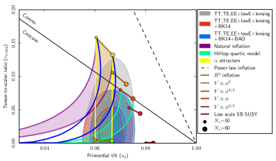
To check these general expectations, we begin with evaluation of $n_{s}$ and $r$ for the Coleman-Weinberg potential (11). The results of our analysis are shown by two thick blue lines in Fig. 4, for $N=50$ (left line) and $N=60$ (right line). As one can see, the area between these lines only minimally overlaps with the 1$\sigma$ region favored by the Planck data. Thus this model is considerably disfavored as compared to the (unphysical) hilltop model shown by the green area in this figure.

Figure 5: Thick red lines falling down from the two yellow circles correspond to $n_{s}$ and $r$ for the regularized hilltop potential (14) for $N=50$ (left line) and $N=60$ (right line).

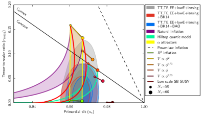
Fig. 5 describes $n_{s}$ and $r$ for the hilltop potential (14) for $n=4$. The thick red lines correspond to $n_{s}$ and $r$ for $N=50$ (the left line) and $N=60$ (the right line). As one can see, the predictions of this model for $n_{s}>0.94$ are quite different from the predictions of the unphysical model (13), but it provides a better fit to the Planck 2018 data than the Coleman-Weinberg model (11). However, whereas one can find some physical motivation for the Coleman-Weinberg model (scale invariance broken by quantum corrections), the model (14) looks rather ad hoc, being specifically designed to mitigate the problems of the hilltop models (13).

One can avoid this conclusion by introducing additional mass parameters, or by considerably modifying the general structure of the potential, but in this paper we are trying to concentrate on relatively simple models which do not require additional parameters, twists and turns for explanation of the observational data.

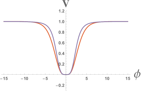
Nothing can explain this point better than an explicit example of a theory which can preserve the predictions of the naive hilltop model (13) while providing vacuum stabilization at $V=0$. To do it, one should keep the potential $1-{\phi^{4}\over m^{4}}$ intact all the way down to a small vicinity of $\phi=m$, and then force the potential to turn up very sharply. Here is the simplest potential satisfying this property that we were able to invent:

$$V_{\rm mod}=V_{0}\,\Bigl{(}\sqrt{{c^{2}}+\Bigl{(}1-{\phi^{4}\over m^{4}}\Bigr{)}^{2}}-{c}\Bigr{)}.$$ (15)

Here $c$ is a small positive constant, which is introduced to make the potential smooth at its minimum at $\phi=m$. The potential $V_{\rm mod}$ is everywhere positive. In the limit $c\ll m^{{-1}}$, this potential (15) is equal to the absolute value of the potential (13), see Fig. 6.

Figure 6: The hilltop potential $V_{0}(1-{\phi^{4}\over m^{4}})$ (13) unbounded from below is shown by the green line for $V_{0}=1$. The strongly modified hilltop potential (15) is shown by the red line for $m=30$, $c=m^{{-1}}$.

Predictions of this theory for $c\lesssim m^{{-1}}$ are well described by the green area in Fig. 1. This potential contains the potential (14) under the square root. But if, as we admitted, the potential (14) is not well motivated, then it is hard to say anything positive about the potential (15). It is constructed by a set of additional manipulations with the potential (14), with the sole purpose to save the predictions of the physically inconsistent models (13). But why would anybody want to do it?

One can summarize these considerations as follows. The reason why the original hilltop models (12) with $n=4$ and $m\lesssim 1$ were popular and deserved to be a target for future searches was that they were ultimately simple. One could modify the shape of the potential at $\phi\sim m$ without modifying its inflationary predictions, and the value of $r=8{m^{4}\over N^{3}}$ could be easily changed by varying $m$ without affecting the attractor value $n_{s}=1-3/N$. This value of $n_{s}$ was consistent with WMAP.

However, the spectral index $n_{s}=1-3/N$ was only marginally consistent with Planck 2013, and it was finally ruled out by Planck 2015 and Planck 2018. In this sense, the original beauty of hilltop models is long gone. The simplest attempts to cure the problems of the hilltop models (13) with $n=4$ lead to a family of models with the predictions interpolating between two bad attractor points. In the limit $m\ll 1$ these models predict unacceptably small $n_{s}$, whereas in the large $m$ limit they predict unacceptably large $r=8/N$, two times greater than the predictions of the simplest (but inconsistent) hilltop model (13).

One can design the models providing a good fit to the data, such as (14), but the predictions of such models are mostly determined not by the structure of the potential at the hilltop, but by the previously unspecified model-dependent terms shown by … in (12). And their predictions are very different from the predictions of the original hilltop inflation models (13) shown by the green area in Fig. 1. One can further modify these models, by requiring that their predictions should be consistent with the predictions of the models (13) with a potential unbounded from below, but this additional requirement is unmotivated. Therefore we would argue the green area in Fig. 1 does not properly represent predictions of the simplest consistent hilltop models discussed in Akrami:2018odb .

And this is not the only problem of the hilltop models. Inflationary predictions described here where evaluated under the assumption that inflation begins at the hilltop. Whereas it is possible for inflation to begin at a local maximum of a potential even if its height is 10 orders of magnitude below the Planck density Linde:2004nz ; Linde:2014nna ; East:2015ggf ; Linde:2017pwt , it is arguably much simpler for inflation to begin at the nearly Planckian density, as in the simplest versions of chaotic inflation Linde:1983gd ; Linde:2005ht . This may happen in the models (11) and (14) if inflation begins at $\phi\gg m$. But in that case inflation ends at $\phi>m$, and the field never rolls up to the hilltop at $\phi=0$ to start a new stage of inflation there. Therefore inflationary predictions become similar to the predictions of the chaotic inflation models $\phi^{n}$ with $n>2$. Such models are already ruled out.

Thus to make the hilltop models attractive one should modify them even further, in order to prevent inflation starting at $\phi\gg m$. There are many ways to do it, for example by making the potentials exponentially steep at $\phi\gg m$, but this would make consistent models of hilltop inflation even more contrived.

4 D-brane inflation

The string theory origin of D-brane inflation model is often attributed to the KKLMMT model Kachru:2003sx , where D3-brane - $\overline{\rm D3}$-brane interaction was studied in the context of the volume modulus stabilization. Earlier proposals for D-brane inflation relevant to our current discussion were made in Dvali:2001fw ; Burgess:2001fx ; GarciaBellido:2001ky . Whereas string theory interpretation of D-brane inflation is somewhat unsettled, the positive evaluation of the cosmological consequences of these models in Akrami:2018odb prompted us to revisit them and implement these models in supergravity Kallosh:2018zsi .

We will discuss two classes of these models, using terminology established in Martin:2013tda . The first class of models called BI (for brane inflation) has the Coulomb-type potential

$$V_{{\rm BI}}=V_{0}\left(1-{m^{n}\over\phi^{{n}}}\right)\ .$$ (16)

BI models has a potential unbounded from below. In the large $m$ limit predictions of these models coincide with the predictions of the theory with a linear potential, but BI models suffer from the same problem as the hilltop inflation (13), and therefore they require a consistent generalization.

This generalization was proposed in the KKLMMT paper Kachru:2003sx where the potential takes a form of the inverse harmonic function; in Martin:2013tda it was called KKLTI (for KKLT inflation):

$$V_{KKLTI}=V_{0}\left(1+{m^{n}\over\phi^{{n}}}\right)^{{-1}}=V_{0}\,{\phi^{n}\over\phi^{n}+m^{n}}\ .$$ (17)

Similar potentials may appear in a different context as well, see e.g. Dong:2010in and Appendix A in Kallosh:2018zsi .

Figure 7: The red line shows the quartic $\alpha$-attractor potential $V=\tanh^{4}{\phi\over\sqrt{6\alpha}}$ with $\alpha=1$. The dark blue line shows the KKLTI potential $V={\phi^{4}\over\phi^{4}+m^{4}}$ for $m=2.5$.

It is instructive to compare KKLTI models with $\alpha$-attractors, see Fig. 7. It shows that $\alpha$-attractors and D-brane inflation models have plateau potentials which look very similar, but the KKLTI models have potentials approaching the plateau polynomially rather than exponentially.

In the small $m$ limit, D-brane models behave as cosmological attractors with the attractor point at $n_{s}\approx 1-{2(n+1)\over N(n+2)}$. For odd values of $n$, both BI and KKLTI models have potentials unbounded from below at $\phi<0$ and therefore require further modifications; we will not discuss them here. The most interesting of the KKLTI models is the one with $n=4$, though the model with $n=2$ also deserves attention. For $n=4$ one has at attractor point

$$n_{s}=1-{5\over 3N},\qquad r={4m^{4/3}\over(3N)^{4/3}}\ .$$ (18)

For $n=2$, the attractor is at

$$n_{s}=1-{3\over 2N},\qquad r={\sqrt{2}m\over N^{3/2}}\ .$$ (19)

In the large $m$ limit, the predictions of BI and KKLTI models are very different. Indeed, predictions of the BI models in the large $m$ limit converge to the predictions of the models with $V\sim\phi$. This is as misleading as the similar predictions of the hilltop inflation models (13), which yield $r=4/N$. In the KKLTI models in the large $m$ limit the last 50-60 e-folds of inflation occur at $\phi=O(10)$. Therefore for $m\gg 10$ the last 50-60 e-foldings occur for $1\ll\phi\ll m$, where the KKLTI potential is proportional to $\phi^{n}$. Therefore for $n=2$ in the large $m$ limit of the KKLTI models one has $r=8/N$, and for $n=4$ one has $r=8/N$, which is 4 times greater than the value of $r$ in the large $m$ limit for the unphysical BI models (16).

Figure 8: Red lines correspond to predictions of the BI theory for $n=4$, $N=50$ and $N=60$. This theory is inconsistent and requires modification provided by the KKLTI model. Predictions of the KKLTI model are shown by the thick purple lines converging with the red lines at the attractor points $r=0$, $n_{s}=1-{5\over 3N}$.

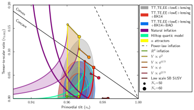
To illustrate this difference, we show the predictions of the BI model and the KKLTI model for $n=4$ in Fig. 8. As one can see, observational predictions of the BI model do not have much in common with the predictions of consistent D-brane models of the type of KKLTI for $r>10^{{-2}}$. The predictions of these models converge at $r\lesssim 10^{{-3}}$ Kallosh:2018zsi . Since this difference of the predictions of KKLTI and BI models is rooted in the physical inconsistency of the BI models, we will no longer investigate BI models in this paper.

It is very instructive to study KKLTI models in parallel with $\alpha$-attractors by plotting their predictions not for $r$ but for $\log_{10}r$, all the way down to $r\sim 10^{{-5}}$, see Fig. 9 taken from our paper with Yusuke Yamada Kallosh:2018zsi .

Figure 9: Comparison of predictions of $\alpha$-attractors and of the D-brane inflationary models within the $2\sigma$ area of the Planck 2018 results for $n_{s}$ and $r$. On the left panel, the dark (light) blue area is the Planck 2018 $1\sigma$ ($2\sigma$) region, with an account taken of the CMB-related data and baryon acoustic oscillations (BAO). The right panel represents the Planck 2018 results based on the CMB related data only, without BAO. These data, without BAO, were used by Planck 2018 in Akrami:2018odb to evaluate inflationary models. Two yellow lines on both panels are for the quadratic T-model of $\alpha$-attractors for $N=50$ and $N=60$. Two purple lines are for the $n=4$ KKLTI model. Two orange lines show the predictions of the $n=2$ KKLTI model.

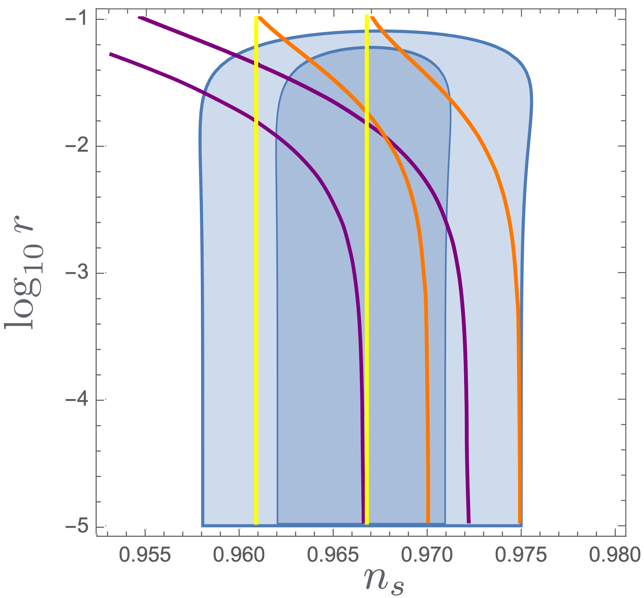
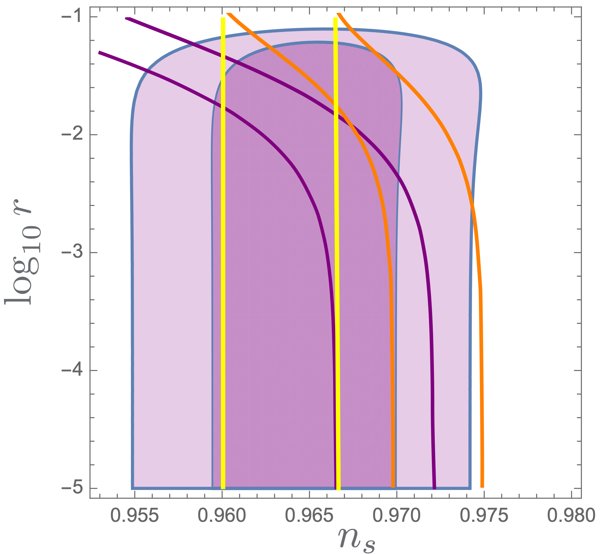
As one can see from Fig. 9, $\alpha$-attractors and KKLTI models can describe arbitrarily small values of $r$. Evaluation of $n_{s}$ for these models in the range of $N$ from 50 to 60 gives us an unexpected numerological bonus: The $\alpha$-attractor prediction $n_{s}=1-{2\over N}$ for $N=60$ exactly coincides with the prediction $n_{s}=1-{5\over 3N}$ of the $n=4$ KKLTI model for $N=50$. Therefore $\alpha$-attractors and KKLTI with $n=4$ stay “shoulder to shoulder”, covering most of the $(n_{s},r)$ space favored by Planck. They miss only a small upper right part of the range of the data favored by Planck 2018, but the KKLTI model with $n=2$ completes this job. As a result, $\alpha$-attractors, in combination with the KKLTI models, almost completely cover the dark blue (red) $1\sigma$ region favored by Planck 2018.

5 Discussion

In this paper we made an attempt to examine the models favored by the latest Planck 2018 data release, including $\alpha$-attractors, hilltop models and D-brane inflation models. Since $\alpha$-attractors were studied in many of our previous papers, we limited ourselves to a brief review of the simplest T-models and E-models in their relation to the Planck 2018 data. We found that a combination of these two basic $\alpha$-attractor models covers a significant part of the area in the ($n_{s},r$) space favored by Planck 2018, see Fig. 2.

The results of our analysis of hilltop models and D-brain models are somewhat unexpected. We were puzzled by the fact that the predictions of the hilltop models $V=V_{0}(1-{\phi^{n}\over m^{{n}}})$, prominently represented by the green area in Fig. 1 (for $n=4$), as well as the predictions of the D-brane inflation models with $V=V_{0}(1-{m^{n}\over\phi^{{n}}})$, in the large $m$ limit converge to the predictions of the simplest inflationary model with a linear potential $V\sim\phi$, as is shown by the thick green lines for the hilltop models in the Fig. 1 and by the thick red lines in 8 for the D-brane models. However, we found that this result is a direct consequence of the unboundedness of these potentials from below.

One can avoid this inconsistency by bending these potentials and creating a minimum at $V=0$. For $m\ll 1$, inflation occurs at $\phi\ll m\ll 1$, so one can modify these models at $\phi\sim m$ without modifying their inflationary predictions. However, the typical hilltop models with $m\lesssim 1$ are ruled out by observations. Meanwhile we found that the improved hilltop models with a minimum at $V=0$ in the large $m$ limit typically predict $r=8/N$, which is way too large. Since the predictions of the simplest consistent versions of the hilltop inflation are considerably different from the predictions of the simplest (but inconsistent) hilltop inflation model $V=V_{0}(1-{\phi^{4}\over m^{{4}}})$ shown by the green area in Fig. 1, we would argue that one should no longer associate hilltop inflation with the green area shown in Fig. 1 in Planck 2018 Akrami:2018odb , as well as in the related figures shown by CMB-S4 and PICO Abazajian:2016yjj ; Abazajian:2019eic ; Hanany:2019lle .

Similarly, the simplest versions of the D-brain inflation with the potential $V=V_{0}(1-{m^{n}\over\phi^{{n}}})$ are physically inconsistent. Consistent generalizations of this model with the positively definite potential Kachru:2003sx in the large $m$ predict unacceptably large $r=4n/N$; see a recent discussion of these models, called KKLTI models, in Kallosh:2018zsi . However, at $m\lesssim 1$ the predictions of the KKLTI models converge to $n_{s}\approx 1-{2(n+1)\over N(n+2)}$, which provides a very good fit to the Planck data for $n=4$, and an acceptably good fit for $n=2$. As one can see from Fig. 9, the simplest $\alpha$-attractors models, in combination with the KKLTI models, almost completely cover the $1\sigma$ region favored by Planck 2018 Kallosh:2018zsi .

The recent Astro2020 Science White Paper “Probing the origin of our Universe through cosmic microwave background constraints on gravitational waves” Shandera:2019ufi suggested that most of the textbook inflation models cannot describe inflation with $r\lesssim 10^{{-3}}$. As one can see from Fig. 9, this problem does not appear in the broad class of $\alpha$-attractor models, as well as in the KKLTI models discussed above. Therefore these two classes of models can be very useful for parametrizing and describing the results of the future search of the gravitational waves produced by inflation, independently of their outcome. We will return to the discussion of this issue in a forthcoming publication.

Acknowledgments: We are grateful to Z. Ahmed, D. Green, F. Finelli, R. Flauger, M. Hazumi, L. Knox, Chao-Lin Kuo, J. Martin, L. Page, L. Senatore, E. Silverstein, V. Vennin, and R. Wechsler for stimulating discussions, and to J. J. Carrasco, S. Ferrara, D. Roest, T. Wrase and Y. Yamada for collaboration on related work. This work is supported by SITP, by the US National Science Foundation grant PHY-1720397 and by the Simons Foundation Origins of the Universe program (Modern Inflationary Cosmology collaboration).

References

- (1) Planck collaboration, Y. Akrami et al., Planck 2018 results. X. Constraints on inflation, 1807.06211.
- (2) Planck collaboration, P. A. R. Ade et al., Planck 2013 results. XXII. Constraints on inflation, Astron. Astrophys. 571 (2014) A22, [1303.5082].
- (3) Planck collaboration, P. A. R. Ade et al., Planck 2015 results. XX. Constraints on inflation, Astron. Astrophys. 594 (2016) A20, [1502.02114].
- (4) CMB-S4 collaboration, K. N. Abazajian et al., CMB-S4 Science Book, First Edition, 1610.02743.
- (5) K. Abazajian et al., CMB-S4 Science Case, Reference Design, and Project Plan, 1907.04473.
- (6) NASA PICO collaboration, S. Hanany et al., PICO: Probe of Inflation and Cosmic Origins, 1902.10541.
- (7) R. Kallosh and A. Linde, Universality Class in Conformal Inflation, JCAP 1307 (2013) 002, [1306.5220].
- (8) R. Kallosh, A. Linde and D. Roest, Universal Attractor for Inflation at Strong Coupling, Phys. Rev. Lett. 112 (2014) 011303, [1310.3950].
- (9) S. Ferrara, R. Kallosh, A. Linde and M. Porrati, Minimal Supergravity Models of Inflation, Phys. Rev. D88 (2013) 085038, [1307.7696].
- (10) R. Kallosh, A. Linde and D. Roest, Superconformal Inflationary -Attractors, JHEP 11 (2013) 198, [1311.0472].
- (11) R. Kallosh, A. Linde and D. Roest, Large field inflation and double -attractors, JHEP 08 (2014) 052, [1405.3646].
- (12) R. Kallosh, A. Linde and D. Roest, The double attractor behavior of induced inflation, JHEP 09 (2014) 062, [1407.4471].
- (13) M. Galante, R. Kallosh, A. Linde and D. Roest, Unity of Cosmological Inflation Attractors, Phys. Rev. Lett. 114 (2015) 141302, [1412.3797].
- (14) A. A. Starobinsky, A New Type of Isotropic Cosmological Models Without Singularity, Phys. Lett. 91B (1980) 99–102.
- (15) D. S. Salopek, J. R. Bond and J. M. Bardeen, Designing Density Fluctuation Spectra in Inflation, Phys. Rev. D40 (1989) 1753.
- (16) F. L. Bezrukov and M. Shaposhnikov, The Standard Model Higgs boson as the inflaton, Phys. Lett. B659 (2008) 703–706, [0710.3755].
- (17) J. J. M. Carrasco, R. Kallosh, A. Linde and D. Roest, Hyperbolic geometry of cosmological attractors, Phys. Rev. D92 (2015) 041301, [1504.05557].
- (18) A. S. Goncharov and A. D. Linde, Chaotic Inflation of the Universe in Supergravity, Sov. Phys. JETP 59 (1984) 930–933.
- (19) A. Linde, Does the first chaotic inflation model in supergravity provide the best fit to the Planck data?, JCAP 1502 (2015) 030, [1412.7111].
- (20) A. D. Linde, A New Inflationary Universe Scenario: A Possible Solution of the Horizon, Flatness, Homogeneity, Isotropy and Primordial Monopole Problems, Phys. Lett. B108 (1982) 389–393.
- (21) W. H. Kinney and K. T. Mahanthappa, Inflation at low scales: General analysis and a detailed model, Phys. Rev. D53 (1996) 5455–5467, [hep-ph/9512241].
- (22) L. Boubekeur and D. H. Lyth, Hilltop inflation, JCAP 0507 (2005) 010, [hep-ph/0502047].
- (23) G. R. Dvali, Q. Shafi and S. Solganik, D-brane inflation, in 4th European Meeting From the Planck Scale to the Electroweak Scale (Planck 2001) La Londe les Maures, Toulon, France, May 11-16, 2001, 2001, hep-th/0105203.
- (24) C. P. Burgess, M. Majumdar, D. Nolte, F. Quevedo, G. Rajesh and R.-J. Zhang, The Inflationary brane anti-brane universe, JHEP 07 (2001) 047, [hep-th/0105204].
- (25) J. Garcia-Bellido, R. Rabadan and F. Zamora, Inflationary scenarios from branes at angles, JHEP 01 (2002) 036, [hep-th/0112147].
- (26) S. Kachru, R. Kallosh, A. D. Linde, J. M. Maldacena, L. P. McAllister and S. P. Trivedi, Towards inflation in string theory, JCAP 0310 (2003) 013, [hep-th/0308055].
- (27) J. Martin, C. Ringeval and V. Vennin, Encyclopædia Inflationaris, Phys. Dark Univ. 5-6 (2014) 75–235, [1303.3787].
- (28) R. Kallosh, A. Linde and Y. Yamada, Planck 2018 and Brane Inflation Revisited, JHEP 01 (2019) 008, [1811.01023].
- (29) R. Kallosh and A. Linde, Escher in the Sky, Comptes Rendus Physique 16 (2015) 914–927, [1503.06785].
- (30) R. Kallosh and A. Linde, Cosmological Attractors and Asymptotic Freedom of the Inflaton Field, JCAP 1606 (2016) 047, [1604.00444].
- (31) G. N. Felder, A. V. Frolov, L. Kofman and A. D. Linde, Cosmology with negative potentials, Phys. Rev. D66 (2002) 023507, [hep-th/0202017].
- (32) A. D. Linde, Creation of a compact topologically nontrivial inflationary universe, JCAP 0410 (2004) 004, [hep-th/0408164].
- (33) A. Linde, Inflationary Cosmology after Planck 2013, in Proceedings, 100th Les Houches Summer School: Post-Planck Cosmology: Les Houches, France, July 8 - August 2, 2013, pp. 231–316, 2015, 1402.0526, DOI.
- (34) W. E. East, M. Kleban, A. Linde and L. Senatore, Beginning inflation in an inhomogeneous universe, JCAP 1609 (2016) 010, [1511.05143].
- (35) A. Linde, On the problem of initial conditions for inflation, in Black Holes, Gravitational Waves and Spacetime Singularities Rome, Italy, May 9-12, 2017, 2017, 1710.04278, http://inspirehep.net/record/1630432/files/arXiv:1710.04278.pdf.
- (36) A. D. Linde, Chaotic Inflation, Phys. Lett. B129 (1983) 177–181.
- (37) A. D. Linde, Particle physics and inflationary cosmology, Contemp. Concepts Phys. 5 (1990) 1–362, [hep-th/0503203].
- (38) X. Dong, B. Horn, E. Silverstein and A. Westphal, Simple exercises to flatten your potential, Phys. Rev. D84 (2011) 026011, [1011.4521].
- (39) S. Shandera et al., Probing the origin of our Universe through cosmic microwave background constraints on gravitational waves, 1903.04700.