Strong and Simple Baselines for Multimodal Utterance Embeddings

Abstract

Human language is a rich multimodal signal consisting of spoken words, facial expressions, body gestures, and vocal intonations. Learning representations for these spoken utterances is a complex research problem due to the presence of multiple heterogeneous sources of information. Recent advances in multimodal learning have followed the general trend of building more complex models that utilize various attention, memory and recurrent components. In this paper, we propose two simple but strong baselines to learn embeddings of multimodal utterances. The first baseline assumes a conditional factorization of the utterance into unimodal factors. Each unimodal factor is modeled using the simple form of a likelihood function obtained via a linear transformation of the embedding. We show that the optimal embedding can be derived in closed form by taking a weighted average of the unimodal features. In order to capture richer representations, our second baseline extends the first by factorizing into unimodal, bimodal, and trimodal factors, while retaining simplicity and efficiency during learning and inference. From a set of experiments across two tasks, we show strong performance on both supervised and semi-supervised multimodal prediction, as well as significant (10 times) speedups over neural models during inference. Overall, we believe that our strong baseline models offer new benchmarking options for future research in multimodal learning.

1 Introduction

Human language is a rich multimodal signal consisting of spoken words, facial expressions, body gestures, and vocal intonations (Streeck and Knapp, 1992). At the heart of many multimodal modeling tasks lies the challenge of learning rich representations of spoken utterances from multiple modalities (Papo et al., 2014). However, learning representations for these spoken utterances is a complex research problem due to the presence of multiple heterogeneous sources of information (Baltrušaitis et al., 2017). This challenging yet crucial research area has real-world applications in robotics (Montalvo et al., 2017; Noda et al., 2014), dialogue systems (Johnston et al., 2002; Rudnicky, 2005), intelligent tutoring systems (Mao and Li, 2012; Banda and Robinson, 2011; Pham and Wang, 2018), and healthcare diagnosis (Wentzel and van der Geest, 2016; Lisetti et al., 2003; Sonntag, 2017). Recent progress on multimodal representation learning has investigated various neural models that utilize one or more of attention, memory and recurrent components (Yang et al., 2017; Liang et al., 2018). There has also been a general trend of building more complicated models for improved performance.

In this paper, we propose two simple but strong baselines to learn embeddings of multimodal utterances. The first baseline assumes a factorization of the utterance into unimodal factors conditioned on the joint embedding. Each unimodal factor is modeled using the simple form of a likelihood function obtained via a linear transformation of the utterance embedding. We derive a coordinate-ascent style algorithm (Wright, 2015) to learn the optimal multimodal embeddings under our model. We show that, under some assumptions, maximum likelihood estimation for the utterance embedding can be derived in closed form and is equivalent to computing a weighted average of the language, visual and acoustic features. Only a few linear transformation parameters need to be learned. In order to capture bimodal and trimodal representations, our second baseline extends the first one by assuming a factorization into unimodal, bimodal, and trimodal factors Zadeh et al. (2017). To summarize, our simple baselines 1) consist primarily of linear functions, 2) have few parameters, and 3) can be approximately solved in a closed form solution. As a result, they demonstrate simplicity and efficiency during learning and inference.

We perform a set of experiments across two tasks and datasets spanning multimodal personality traits recognition Park et al. (2014) and multimodal sentiment analysis (Zadeh et al., 2016). Our proposed baseline models 1) achieve competitive performance on supervised multimodal learning, 2) improve upon classical deep autoencoders for semi-supervised multimodal learning, and 3) are up to 10 times faster during inference. Overall, we believe that our baseline models offer new benchmarks for future multimodal research.

2 Related Work

We provide a review of sentence embeddings, multimodal utterance embeddings, and strong baselines.

2.1 Language-Based Sentence Embeddings

Sentence embeddings are crucial for down-stream tasks such as document classification, opinion analysis, and machine translation. With the advent of deep neural networks, multiple network designs such as Recurrent Neural Networks (RNNs) Rumelhart et al. (1986), Long-Short Term Memory networks (LSTMs) Hochreiter and Schmidhuber (1997), Temporal Convolutional Networks Bai et al. (2018), and the Transformer Vaswani et al. (2017) have been proposed and achieve superior performance. However, more training data is required for larger models Peters et al. (2018). In light of this challenge, researchers have started to leverage unsupervised training objectives to learn sentence embedding which showed state-of-the-art performance across multiple tasks Devlin et al. (2018). In our paper, we go beyond unimodal language-based sentence embeddings and consider multimodal spoken utterances where additional information from the nonverbal behaviors is crucial to infer speaker intent.

2.2 Multimodal Utterance Embeddings

Learning multimodal utterance embeddings brings a new level of complexity as it requires modeling both intra-modal and inter-modal interactions Liang et al. (2018). Previous approaches have explored variants of graphical models and neural networks for multimodal data. RNNs (Elman, 1990; Jain and Medsker, 1999), LSTMs Hochreiter and Schmidhuber (1997), and convolutional neural networks Krizhevsky et al. (2012) have been extended for multimodal settings Rajagopalan et al. (2016); Lee et al. (2018). Experiments on more advanced networks suggested that encouraging correlation between modalities Yang et al. (2017), enforcing disentanglement on multimodal representations Tsai et al. (2018), and using attention to weight modalities Gulrajani et al. (2017) led to better performing multimodal representations. In our paper, we present a new perspective on learning multimodal utterance embeddings by assuming a conditional factorization over the language, visual and acoustic features. Our simple but strong baseline models offer an alternative approach that is extremely fast and competitive on both supervised and semi-supervised prediction tasks.

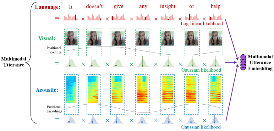
Figure 1: Our baseline model assumes a factorization of the multimodal utterance into unimodal factors conditioned on the joint utterance embedding. Each unimodal factor is modeled using the simple form of a likelihood function obtained via a linear transformation of the utterance embedding. We show that, under some assumptions, maximum likelihood estimation for the utterance embedding can be derived in closed form and is equivalent to taking a weighted average of the language, visual and acoustic features.

2.3 Strong Baseline Models

A recent trend in NLP research has been geared towards building simple but strong baselines Arora et al. (2017); Shen et al. (2018); Wieting and Kiela (2019); Denkowski and Neubig (2017). The effectiveness of these baselines indicate that complicated network components are not always required. For example, Arora et al. (2017) constructed sentence embeddings from weighted combinations of word embeddings which requires no trainable parameters yet generalizes well to down-stream tasks. Shen et al. (2018) proposed parameter-free pooling operations on word embeddings for document classification, text sequence matching, and text tagging. Wieting and Kiela (2019) discovered that random sentence encoders achieve competitive performance as compared to larger models that involve expensive training and tuning. Denkowski and Neubig (2017) emphasized the importance of choosing a basic neural machine translation model and carefully reporting the relative gains achieved by the proposed techniques. Authors in other domains have also highlighted the importance of developing strong baselines Lakshminarayanan et al. (2017); Sharif Razavian et al. (2014). To the best of our knowledge, our paper is the first to propose and evaluate strong, non-neural baselines for multimodal utterance embeddings.

3 Baselines for Multimodal Learning

3.1 Notation

Suppose we are given video data where each utterance segment is denoted as $\mathbf{s}$. Each segment contains individual words $w$ in a sequence $\mathbf{w}$, visual features $v$ in a sequence $\mathbf{v}$, and acoustic features $a$ in a sequence $\mathbf{a}$. We aim to learn a representation $m_{\mathbf{s}}$ for each segment that summarizes information present in the multimodal utterance.

3.2 Background

Our model is related to the work done by Arora et al. (2016) and Arora et al. (2017). In the following, we first provide a brief review of their method. Given a sentence, Arora et al. (2016) aims to learn a sentence embedding $c_{s}$. They do so by assuming that the probability of observing a word $w_{t}$ at time $t$ is given by a log-linear word production model (Mnih and Hinton, 2007) with respect to $c_{s}$:

$$\mathbb{P}[\textrm{$w_{t}$}|c_{s}]=\frac{\exp\left(\langle v_{w_{t}},c_{s}\rangle\right)}{Z_{c_{s}}},$$ (1)

where $c_{s}$ is the sentence embedding (context), $v_{w_{t}}$ represents the word vector associated with word $w_{t}$ and $Z_{c_{s}}=\sum_{w\in V}\exp\left(\langle v_{w},c_{s}\rangle\right)$ is a normalizing constant over all words in the vocabulary. Given this posterior probability, the desired sentence embedding $c_{s}$ can be obtained by maximizing Equation (1) with respect to $c_{s}$. Under some assumptions on $c_{s}$, this maximization yields a closed-form solution which provides an efficient learning algorithm for sentence embeddings.

Arora et al. (2017) further extends this model by introducing a “smoothing term” $\alpha$ to account for the production of frequent stop words or out of context words independent of the discourse vector. Given estimated unigram probabilities $p(w)$, the probability of a word at time $t$ is given by

$$\mathbb{P}[\textrm{$w_{t}$}|c_{s}]=\alpha p(w_{t})+(1-\alpha)\frac{\exp\left(\langle v_{w_{t}},c_{s}\rangle\right)}{Z_{c_{s}}}.$$ (2)

Under this model with the additional hyperparameter $\alpha$, we can still obtain a closed-form solution for the optimal $c_{s}$.

3.3 Baseline 1: Factorized Unimodal Model

In this subsection, we outline our method for learning representations of multimodal utterances. An overview of our proposed baseline model is shown in Figure 1. Our method begins by assuming a factorization of the multimodal utterance into unimodal factors conditioned on the joint utterance embedding. Next, each unimodal factor is modeled using the simple form of a likelihood function obtained via a linear transformation of the utterance embedding. Finally, we incorporate positional encodings to represent temporal information in the features. We first present the details of our proposed baseline before deriving a coordinate ascent style optimization algorithm to learn utterance embeddings in our model.

Unimodal Factorization: We use $m_{\mathbf{s}}$ to represent the multimodal utterance embedding. To begin, we simplify the composition of $m_{\mathbf{s}}$ by assuming that the segment $\mathbf{s}$ can be conditionally factorized into words ($\mathbf{w}$), visual features ($\mathbf{v}$), and acoustic features ($\mathbf{a}$). Each factor is also associated with a temperature hyperparameter ($\alpha_{\mathbf{w}}$, $\alpha_{\mathbf{v}}$, $\alpha_{\mathbf{a}}$) that represents the contribution of each factor towards the multimodal utterance. The likelihood of a segment $\mathbf{s}$ given the embedding $m_{\mathbf{s}}$ is therefore

$$\mathbb{P}[\mathbf{s}|m_{\mathbf{s}}]=\mathbb{P}[\mathbf{w}|m_{\mathbf{s}}]^{\alpha_{\mathbf{w}}}\left(\mathbb{P}[\mathbf{v}|m_{\mathbf{s}}]\right)^{\alpha_{\mathbf{v}}}\mathbb{P}[\mathbf{a}|m_{\mathbf{s}}]^{\alpha_{\mathbf{a}}}$$

$$=\prod_{w\in\mathbf{w}}\mathbb{P}[w|m_{\mathbf{s}}]^{\alpha_{\mathbf{w}}}\prod_{v\in\mathbf{v}}\mathbb{P}[v|m_{\mathbf{s}}]^{\alpha_{\mathbf{v}}}\prod_{a\in\mathbf{a}}\mathbb{P}[a|m_{\mathbf{s}}]^{\alpha_{\mathbf{a}}}.$$ (3)

Choice of Likelihood Functions: As suggested by Arora et al. (2017), given $m_{\mathbf{s}}$, we model the probability of a word $w$ using Equation (2). In order to analytically solve for ${m_{\mathbf{s}}}$, a lemma is introduced by Arora et al. (2016, 2017) which states that the partition function $Z_{{m_{\mathbf{s}}}}$ is concentrated around some constant $Z$ (for all $m_{\mathbf{s}}$). This lemma is also known as the “self-normalizing” phenomenon of log-linear models (Andreas and Klein, 2015; Andreas et al., 2015). We use the same assumption and treat $Z_{{m_{\mathbf{s}}}_{t}}\approx Z$ for all $m_{\mathbf{s}}$.

Unlike discrete text tokens, the visual features are continuous. We assume that the visual features are generated from an isotropic Gaussian distribution. In section 5.1, we visually analyze the distribution of the features for real world datasets and show that these likelihood modeling assumptions are indeed justified. The Gaussian distribution is parametrized by simple linear transformations $W_{v}^{\mu},W_{v}^{\sigma}\in\mathbb{R}^{|v|\times|m_{\mathbf{s}}|}$ and $b_{v}^{\mu},b_{v}^{\sigma}\in\mathbb{R}^{|v|}$:

$$v|m_{\mathbf{s}} \sim\mathcal{N}(\mu_{v},\sigma_{v}^{2}),$$ (4)

$$\mu_{v} =W_{v}^{\mu}m_{\mathbf{s}}+b_{v}^{\mu},$$ (5)

$$\sigma_{v} =\textrm{diag}\left(\exp\left(W_{v}^{\sigma}m_{\mathbf{s}}+b_{v}^{\sigma}\right)\right).$$ (6)

Similarly, we also assume that the continuous acoustic features are generated from a different isotropic Gaussian distribution parametrized as:

$$a|m_{\mathbf{s}} \sim\mathcal{N}(\mu_{a},\sigma_{a}^{2}),$$ (7)

$$\mu_{a} =W_{a}^{\mu}m_{\mathbf{s}}+b_{a}^{\mu},$$ (8)

$$\sigma_{a} =\textrm{diag}\left(\exp\left(W_{a}^{\sigma}m_{\mathbf{s}}+b_{a}^{\sigma}\right)\right).$$ (9)

Positional Encodings: Finally, we incorporate positional encodings Vaswani et al. (2017) into the features to represent temporal information. We use $d$-dimensional positional encodings with entries:

$$PE_{pos,2i} =\sin\left(pos/10000^{2i/d}\right),$$ (10)

$$PE_{pos,2i+1} =\cos\left(pos/10000^{2i/d}\right).$$ (11)

where $pos$ is the position (time step) and $i\in[1,d]$ indexes the dimension of the positional encodings. We call this resulting model Multimodal Baseline 1 (MMB1).

3.4 Optimization for Baseline 1

We define our objective function by the log-likelihood of the observed multimodal utterance $\mathbf{s}$. The maximum likelihood estimator of the utterance embedding $m_{\mathbf{s}}$ and the linear transformation parameters $W$ and $b$ can then be obtained by maximizing this objective

$$\mathcal{L}(m_{\mathbf{s}},W,b;\mathbf{s}) =\log\mathbb{P}[\mathbf{s}|m_{\mathbf{s}};W,b],$$ (12)

where we use $W$ and $b$ to denote all linear transformation parameters.

Coordinate Ascent Style Algorithm: Since the objective (12) is not jointly convex in $m_{\mathbf{s}}$, $W$ and $b$, we optimize by alternating between: 1) solving for $m_{\mathbf{s}}$ given the parameters $W$ and $b$ at the current iterate, and 2) given $m_{\mathbf{s}}$, updating $W$ and $b$ using a gradient-based algorithm. This resembles the coordinate ascent optimization algorithm which maximizes the objective according to each coordinate separately (Tseng, 2001; Wright, 2015). Algorithm 1 presents our method for learning utterance embeddings. In the following sections, we describe how to solve for $m_{\mathbf{s}}$ and update $W$ and $b$.

Algorithm 1 Baseline 1

1:procedure Baseline 1

2:     Initialize $m_{\mathbf{s}},W,b$.

3:     for each iteration do

4:         Fix $W^{(k)},b^{(k)}$, compute $m_{\mathbf{s}}^{(k)}$ by (1).

5:         Fix $m_{\mathbf{s}}^{(k)}$, compute $\nabla_{W}\mathcal{L}$ by (21-1).

6:         Fix $m_{\mathbf{s}}^{(k)}$, compute $\nabla_{b}\mathcal{L}$ by (23-1).

7:         Update $W^{(k+1)}$ from $W^{(k)}$ and $\nabla_{W}\mathcal{L}$.

8:         Update $b^{(k+1)}$ from $b^{(k)}$ and $\nabla_{b}\mathcal{L}$.      

Solving for $m_{\mathbf{s}}$: We first derive an algorithm to solve for the optimal $m_{\mathbf{s}}$ given the log likelihood objective in (12), and parameters $W$ and $b$.

Theorem 1.

[Solving for $m_{\mathbf{s}}$] Assume the optimal $m_{\mathbf{s}}$ lies on the unit sphere (i.e. $\|m_{\mathbf{s}}\|_{2}^{2}=1$), then closed form of $m_{\mathbf{s}}$ in line 4 in Algorithm 1 is

$$m_{\mathbf{s}}^{*} =\sum_{w\in s}\psi_{w}w$$

$$+\sum_{v\in s}\left(W_{v}^{\mu\top}\tilde{v}^{(1)}\psi_{v}^{(1)}+W_{v}^{\sigma\top}\tilde{v}^{(2)}\psi_{v}^{(2)}\right)$$

$$+\sum_{a\in s}\left(W_{a}^{\mu\top}\tilde{a}^{(1)}\psi_{a}^{(1)}+W_{a}^{\sigma\top}\tilde{a}^{(2)}\psi_{a}^{(2)}\right).$$ (13)

where the shifted visual and acoustic features are:

$$\tilde{v}^{(1)}=v-b_{v}^{\mu},\ \tilde{v}^{(2)}=(v-b_{v}^{\mu})\otimes(v-b_{v}^{\mu}),$$ (14)

$$\tilde{a}^{(1)}=a-b_{a}^{\mu},\ \tilde{a}^{(2)}=(a-b_{a}^{\mu})\otimes(a-b_{a}^{\mu}),\vspace{-0mm}$$ (15)

where $\otimes$ denotes Hadamard (element-wise) product and the weights $\psi$’s are given as follows:

$$\psi_{w} =\frac{{\alpha_{\mathbf{w}}}(1-\alpha)/(\alpha Z)}{p(w)+(1-\alpha)/(\alpha Z)},$$ (16)

$$\psi_{v}^{(1)} =\textup{diag}\left(\frac{\alpha_{\mathbf{v}}}{\exp\left(2b_{v}^{\sigma}\right)}\right),$$ (17)

$$\psi_{v}^{(2)} =\textup{diag}\left(\frac{\alpha_{\mathbf{v}}}{\exp\left(2b^{\sigma}_{v}\right)}-\alpha_{\mathbf{v}}\right),$$ (18)

$$\psi_{a}^{(1)} =\textup{diag}\left(\frac{\alpha_{\mathbf{a}}}{\exp\left(2b_{a}^{\sigma}\right)}\right),$$ (19)

$$\psi_{a}^{(2)} =\textup{diag}\left(\frac{\alpha_{\mathbf{a}}}{\exp\left(2b^{\sigma}_{a}\right)}-\alpha_{\mathbf{a}}\right).$$ (20)

Proof.

The proof is adapted from Arora et al. (2017) and involves computing the gradients $\nabla_{m_{\mathbf{s}}}\log\mathbb{P}[\cdot|m_{\mathbf{s}}]^{\alpha_{\mathbf{\cdot}}}$. We express $\log\mathbb{P}[\cdot|m_{\mathbf{s}}]$ via a Taylor expansion approximation and we observe that $\log\mathbb{P}[\cdot|m_{\mathbf{s}}]\approx c+\langle m_{\mathbf{s}},g\rangle$ for a constant $c$ and a vector $g$. Then, we can obtain $m_{\mathbf{s}}^{*}$ by computing $\operatorname*{arg\,max}_{m_{\mathbf{s}}^{*}}\mathcal{L}(m_{\mathbf{s}},W,b;\mathbf{s})$ which yields a closed-form solution. Please refer to the supplementary material for proof details. ∎

Observe that the optimal embedding $m_{\mathbf{s}}^{*}$ is a weighted average of the word features $w$ and the (shifted and transformed) visual and acoustic features, $\tilde{v}$ and $\tilde{a}$. Our choice of a Gaussian likelihood for the visual and acoustic features introduces a squared term $(v-b_{v}^{\mu})\otimes(v-b_{v}^{\mu})$ to account for the $\ell_{2}$ distance present in the pdf. The transformation matrix $W^{\top}$ transforms the visual and acoustic features into the multimodal embedding space. Regarding the weights $\psi$, note that: 1) the weights are proportional to the global temperatures $\alpha$ assigned to that modality, 2) the weights $\psi_{w}$ are inversely proportional to $p(w)$ (rare words carry more weight), and 3) the weights $\psi_{v}$ and $\psi_{a}$ scale each feature dimension inversely by their magnitude.

Updating $W$ and $b$: To find the optimal linear transformation parameters $W$ and $b$ to maximize the objective in (12), we perform gradient-based optimization on $W$ and $b$ (in Algorithm 1 line 5-8).

Proposition 1.

[Updating $W$ and $b$] The gradients $\nabla_{W}\mathcal{L}(m_{\mathbf{s}},W,b)$ and $\nabla_{b}\mathcal{L}(m_{\mathbf{s}},W,b)$, in each dimension, are:

$$\nabla_{{W^{\mu}_{v}}_{ij}}\mathcal{L}(m_{\mathbf{s}},W,b) =\alpha_{\mathbf{v}}\textup{tr}\left[\left(\sigma_{v}^{-2}(v-\mu_{v})\right)^{\top}{m_{\mathbf{s}}}_{j}\right],$$ (21)

$$\nabla_{{W^{\sigma}_{v}}_{ij}}\mathcal{L}(m_{\mathbf{s}},W,b)=$$

$$-\frac{\alpha_{\mathbf{v}}}{2}\textup{tr}\left[\left(\sigma_{v}^{-2}-\sigma_{v}^{-2}(v-\mu_{v})(v-\mu_{v})^{\top}\sigma_{v}^{-2}\right)^{\top}{\sigma_{v}}_{ii}{m_{\mathbf{s}}}_{j}\right],$$ (22)

$$\nabla_{{b^{\mu}_{v}}_{i}}\mathcal{L}(m_{\mathbf{s}},W,b) =\alpha_{\mathbf{v}}\textup{tr}\left[\left(\sigma_{v}^{-2}(v-\mu_{v})\right)^{\top}\right],$$ (23)

$$\nabla_{{b^{\sigma}_{v}}_{i}}\mathcal{L}(m_{\mathbf{s}},W,b)$$

$$=-\frac{\alpha_{\mathbf{v}}}{2}\textup{tr}\left[\left(\sigma_{v}^{-2}-\sigma_{v}^{-2}(v-\mu_{v})(v-\mu_{v})^{\top}\sigma_{v}^{-2}\right)^{\top}{\sigma_{v}}_{ii}\right].$$ (24)

Proof.

The proof involves differentiating the log likelihood of a multivariate Gaussian with respect to $\mu$ and $\sigma$ before applying the chain rule to $\mu=W^{\mu}m_{\mathbf{s}}+b^{\mu}$ and $\sigma=\textrm{diag}\left(\exp\left(W^{\sigma}m_{\mathbf{s}}+b^{\sigma}\right)\right)$. ∎

3.5 Baseline 2: Incorporating Bimodal and Trimodal Interactions

So far, we have assumed the utterance segment $s$ can be independently factorized into unimodal features. In this subsection, we extend the setting to take account for bimodal and trimodal interactions. We adopt the idea of early-fusion (Srivastava and Salakhutdinov, 2012), which means the bimodal and trimodal interactions are captured by the concatenated features from different modalities. Specifically, we define our factorized model as:

$$\mathbb{P}[\mathbf{s}|m_{\mathbf{s}}]=\mathbb{P}[\mathbf{w}|m_{\mathbf{s}}]^{\alpha_{\mathbf{w}}}\mathbb{P}[\mathbf{v}|m_{\mathbf{s}}]^{\alpha_{\mathbf{v}}}\mathbb{P}[\mathbf{a}|m_{\mathbf{s}}]^{\alpha_{\mathbf{a}}}$$

$$\mathbb{P}[\left(\mathbf{w}\oplus\mathbf{v}\right)|m_{\mathbf{s}}]^{\alpha_{\mathbf{wv}}}\mathbb{P}[\left(\mathbf{w}\oplus\mathbf{a}\right)|m_{\mathbf{s}}]^{\alpha_{\mathbf{wa}}}$$

$$\mathbb{P}[\left(\mathbf{v}\oplus\mathbf{a}\right)|m_{\mathbf{s}}]^{\alpha_{\mathbf{va}}}\mathbb{P}[\left(\mathbf{w}\oplus\mathbf{v}\oplus\mathbf{a}\right)|m_{\mathbf{s}}]^{\alpha_{\mathbf{wva}}},$$ (25)

where $\oplus$ denotes vector concatenation for bimodal and trimodal features. Each of the individual probabilities factorize in the same way as Equation (3.3) (i.e. $\mathbb{P}[\mathbf{a}|m_{\mathbf{s}}]^{\alpha_{\mathbf{a}}}=\prod_{a\in\mathbf{a}}\mathbb{P}[a|m_{\mathbf{s}}]^{\alpha_{\mathbf{a}}}$). Similar to baseline 1, we assume a log-linear likelihood (2) for $\mathbb{P}[{w}|m_{\mathbf{s}}]$ and a Gaussian likelihood (4) for all remaining terms. We call this Multimodal Baseline 2 (MMB2).

3.6 Optimization for Baseline 2

The optimization algorithm derived in section 3.4 can be easily extended to learn $m_{\mathbf{s}}$, $W$ and $b$ in Baseline 2. We again alternate between the 2 steps of 1) solving for $m_{\mathbf{s}}$ given the parameters $W$ and $b$ at the current iterate, and 2) given $m_{\mathbf{s}}$, updating $W$ and $b$ using a gradient-based algorithm.

Solving for $m_{\mathbf{s}}$: We state a result that derives the closed-form of $m_{\mathbf{s}}$ given $W$ and $b$:

Corollary 1.

[Solving for $m_{\mathbf{s}}$] Assume that the optimal $m_{\mathbf{s}}$ lies on the unit sphere (i.e. $\|m_{\mathbf{s}}\|_{2}^{2}=1$). The closed-form (in Algorithm 1 line 4) for $m_{\mathbf{s}}$ is:

$$m_{\mathbf{s}}^{*}=\sum_{w\in\mathbf{w}}\psi_{w}w$$

$$+\sum_{v\in\mathbf{v}}\left(W_{v}^{\mu\top}\tilde{v}^{(1)}\psi_{v}^{(1)}+W_{v}^{\sigma\top}\tilde{v}^{(2)}\psi_{v}^{(2)}\right)$$

$$+\sum_{a\in\mathbf{a}}\left(W_{a}^{\mu\top}\tilde{a}^{(1)}\psi_{a}^{(1)}+W_{a}^{\sigma\top}\tilde{a}^{(2)}\psi_{a}^{(2)}\right)$$

$$+\sum_{\begin{subarray}{c}\mathbf{f}\in\{\mathbf{w}\oplus\mathbf{v},\mathbf{w}\oplus\mathbf{a},\\ \mathbf{v}\oplus\mathbf{a},\mathbf{w}\oplus\mathbf{v}\oplus\mathbf{a}\}\end{subarray}}\sum_{f\in\mathbf{f}}\left(W_{f}^{\mu\top}\tilde{f}^{(1)}\psi_{f}^{(1)}+W_{f}^{\sigma\top}\tilde{f}^{(2)}\psi_{f}^{(2)}\right)$$ (26)

where the shifted (and squared) visual features are:

$$\tilde{v}^{(1)}=v-b_{v}^{\mu},\ \tilde{v}^{(2)}=(v-b_{v}^{\mu})\otimes(v-b_{v}^{\mu}),$$ (27)

(and analogously for $\tilde{f}^{(1)},\tilde{f}^{(2)},f\in\{a,w\oplus v,w\oplus a,v\oplus a,w\oplus v\oplus a\}$). The weights $\psi$’s are:

$$\psi_{w} =\frac{{\alpha_{\mathbf{w}}}(1-\alpha)/(\alpha Z)}{p(w)+(1-\alpha)/(\alpha Z)},$$ (28)

$$\psi_{v}^{(1)} =\textup{diag}\left(\frac{\alpha_{\mathbf{v}}}{\exp\left(2b_{v}^{\sigma}\right)}\right),$$ (29)

$$\psi_{v}^{(2)} =\textup{diag}\left(\frac{\alpha_{\mathbf{v}}}{\exp\left(2b^{\sigma}_{v}\right)}-\alpha_{\mathbf{v}}\right).$$ (30)

(and analogously for $\psi_{f}^{(1)},\psi_{f}^{(2)},f\in\{a,w\oplus v,w\oplus a,v\oplus a,w\oplus v\oplus a\}$).

Proof.

The proof is a symmetric extension of Theorem 1 to take into account the Gaussian likelihoods for bimodal and trimodal features. ∎

Updating $W$ and $b$: The gradient equations for updating $W$ and $b$ are identical to those derived in Proposition 1, Equations (21-1).

3.7 Multimodal Prediction

Given the optimal embeddings $m_{\mathbf{s}}$, we can now train a classifier from $m_{\mathbf{s}}$ to labels $y$ for multimodal prediction. $m_{\mathbf{s}}$ can also be fine-tuned on labeled data (i.e. taking gradient descent steps to update $m_{\mathbf{s}}$ with respect to the task-specific loss functions) to learn task-specific multimodal utterance representations. In our experiments, we use a fully connected neural network for our classifier.

4 Experimental Setup

To evaluate the generalization of our models, we perform experiments on multimodal speaker traits recognition and multimodal sentiment analysis. The code for our experiments is released at https://github.com/yaochie/multimodal-baselines, and all datasets for our experiments can be downloaded at https://github.com/A2Zadeh/CMU-MultimodalSDK.

4.1 Datasets

All datasets consist of monologue videos where the speaker’s intentions are conveyed through the language, visual and acoustic modalities. The multimodal features are described in the next subsection.

Multimodal Speaker Traits Recognition involves recognizing speaker traits based on multimodal utterances. POM Park et al. (2014) contains 903 videos each annotated for speaker traits: confident (con), voice pleasant (voi), dominance (dom), vivid (viv), reserved (res), trusting (tru), relaxed (rel), outgoing (out), thorough (tho), nervous (ner), and humorous (hum). The abbreviations (inside parentheses) are used in the tables.

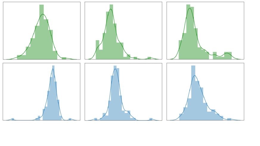
Figure 2: Histogram visualizations of the visual (top) and acoustic (bottom) features in some CMU-MOSI multimodal utterances. Many of the features converge to a Gaussian distribution across the time steps in the utterance, justifying our parametrization for the visual and acoustic likelihood functions.

Dataset	POM Personality Trait Recognition, measured in MAE
Task	Con	Voi	Dom	Viv	Res	Tru	Rel	Out	Tho	Ner	Hum
Majority	1.483	1.089	1.167	1.158	1.166	0.743	0.753	0.872	0.939	1.181	1.774
SVM	1.071	0.938	0.865	1.043	0.877	0.536	0.594	0.702	0.728	0.714	0.801
DF	1.033	0.899	0.870	0.997	0.884	0.534	0.591	0.698	0.732	0.695	0.768
EF-LSTM(⋆)	1.035	0.911	0.880	0.981	0.872	0.556	0.594	0.700	0.712	0.706	0.762
MV-LSTM	1.029	0.971	0.944	0.976	0.877	0.523	0.625	0.703	0.792	0.687	0.770
BC-LSTM	1.016	0.914	0.859	0.905	0.888	0.564	0.630	0.708	0.680	0.705	0.767
TFN	1.049	0.927	0.864	1.000	0.900	0.572	0.621	0.706	0.743	0.727	0.770
MFN	0.952	0.882	0.835	0.908	0.821	0.521	0.566	0.679	0.665	0.654	0.727
MMB2	1.015	0.878	0.885	0.967	0.857	0.522	0.578	0.685	0.705	0.692	0.726

Dataset	POM Personality Trait Recognition, measured in $r$
Task	Con	Voi	Dom	Viv	Res	Tru	Rel	Out	Tho	Ner	Hum
Majority	-0.041	-0.104	-0.031	-0.044	0.006	-0.077	-0.024	-0.085	-0.130	0.097	-0.069
SVM	0.063	-0.004	0.141	0.076	0.134	0.168	0.104	0.066	0.134	0.068	0.147
DF	0.240	0.017	0.139	0.173	0.118	0.143	0.019	0.093	0.041	0.136	0.259
EF-LSTM(⋆)	0.221	0.042	0.151	0.239	0.268	0.069	0.092	0.215	0.252	0.159	0.272
MV-LSTM	0.358	0.131	0.146	0.347	0.323	0.237	0.119	0.238	0.284	0.258	0.317
BC-LSTM	0.359	0.081	0.234	0.417	0.450	0.109	0.075	0.078	0.363	0.184	0.319
TFN	0.089	0.030	0.020	0.204	-0.051	-0.064	0.114	0.060	0.048	-0.002	0.213
MFN	0.395	0.193	0.313	0.431	0.333	0.296	0.255	0.259	0.381	0.318	0.386
MMB2	0.350	0.220	0.333	0.434	0.332	0.176	0.224	0.318	0.394	0.296	0.366

Dataset	CMU-MOSI
Task	Sentiment
Metric	A$({2})$	F1
Majority	50.2	50.1
RF	56.4	56.3
THMM	50.7	45.4
EF-HCRF(⋆)	65.3	65.4
MV-HCRF(⋆)	65.6	65.7
SVM-MD	71.6	72.3
C-MKL	72.3	72.0
DF	72.3	72.1
SAL-CNN	73.0	72.6
EF-LSTM(⋆)	74.3	74.3
MV-LSTM	73.9	74.0
BC-LSTM	73.9	73.9
TFN	74.6	74.5
MFN	77.4	77.3
MMB1	73.6	73.4
MMB2	75.2	75.1

Table 1: Results for multimodal personality trait recognition on POM (left) and multimodal sentiment analysis on CMU-MOSI (right). EF-LSTM^(⋆)and HCRF^(⋆) denote the best result obtained from the LSTM and HCRF variants respectively. The top two results are highlighted in bold. Our proposed baseline model (MMB2), despite its simplicity, often ranks in the top two models and outperforms many large neural models such as C-MKL, DF, SAL-CNN, EF-LSTM, MV-LSTM, BC-LSTM, TFN, and MFN.

Multimodal Sentiment Analysis involves analyzing speaker sentiment based on video content. Multimodal sentiment analysis extends conventional language-based sentiment analysis to a multimodal setup where both verbal and non-verbal signals contribute to the expression of sentiment. We use CMU-MOSI Zadeh et al. (2016) which consists of 2199 opinion segments from online videos each annotated with sentiment from strongly negative $(-3)$ to strongly positive $(+3)$.

4.2 Multimodal Features and Alignment

GloVe word embeddings Pennington et al. (2014), Facet iMotions (2017) and COVAREP Degottex et al. (2014) are extracted for the language, visual and acoustic modalities respectively. Forced alignment is performed using P2FA Yuan and Liberman (2008) to obtain the exact utterance times of each word. The video and audio features are aligned by computing the expectation of their features over each word interval Liang et al. (2018).

4.3 Evaluation Metrics

For classification, we report multiclass classification accuracy A$({c})$ where $c$ denotes the number of classes and F1 score. For regression, we report Mean Absolute Error (MAE) and Pearson’s correlation ($r$). For MAE lower values indicate better performance. For all remaining metrics, higher values indicate better performance.

5 Results and Discussion

5.1 Gaussian Likelihood Assumption

Before proceeding to the experimental results, we perform some sanity checks on our modeling assumptions. We plotted histograms of the visual and acoustic features in CMU-MOSI utterances to visually determine if they resemble a Gaussian distribution. From the plots in Figure 2, we observe that many of the features indeed converge approximately to a Gaussian distribution across the time steps in the utterance, justifying the parametrization for the visual and acoustic likelihood functions in our model.

5.2 Supervised Learning

Our first set of experiments evaluates the performance of our baselines on two multimodal prediction tasks: multimodal sentiment analysis on CMU-MOSI and multimodal speaker traits recognition on POM. On CMU-MOSI (right side of Table 1), our model MMB2 performs competitively against many neural models including early fusion deep neural networks Nojavanasghari et al. (2016), several variants of LSTMs (stacked, bidirectional etc.) (Hochreiter and Schmidhuber, 1997; Schuster and Paliwal, 1997), Multi-view LSTMs Rajagopalan et al. (2016), and tensor product recurrent models (TFN) Zadeh et al. (2017). For multimodal personality traits recognition on POM (left side of Table 1), our baseline is able to additionally outperform more complicated memory-based recurrent models such as MFN (Zadeh et al., 2018) on several metrics. We view this as an impressive achievement considering the simplicity of our model and the significantly fewer parameters that our model contains. As we will later show, our model’s strong performance comes with the additional benefit of being significantly faster than the existing models.

5.3 Semi-supervised Learning

% Labels	Dataset	CMU-MOSI
	Task	Sentiment
	Metric	A$({2})$	F1
40%	AE	55.4	54.7
	seq2seq	56.4	49.3
	MMB2	72.9	72.8
60%	AE	55.2	54.2
	seq2seq	56.3	51.5
	MMB2	73.6	73.5
80%	AE	55.2	54.8
	seq2seq	55.7	54.7
	MMB2	74.1	74.1
100%	AE	55.2	53.2
	seq2seq	57.0	54.1
	MMB2	75.1	75.1

Table 2: Semi-supervised sentiment prediction results on CMU-MOSI. Our model outperforms deep autoencoders (AE) and their recurrent variant (seq2seq), remaining strong despite limited labeled data.

Our next set of experiments evaluates the performance of our proposed baseline models when there is limited labeled data. Intuitively, we expect our model to have a lower sample complexity since training our model involves learning fewer parameters. As a result, we hypothesize that our model will generalize better when there is limited amounts of labeled data as compared to larger neural models with a greater number of parameters.

We test this hypothesis by evaluating the performance of our model on the CMU-MOSI dataset with only 40%, 60%, 80%, and 100% of the training labels. The remainder of the train set now consists of unlabeled data which is also used during training but in a semi-supervised fashion. We use the entire train set (both labeled and unlabeled data) for unsupervised learning of our multimodal embeddings before the embeddings are fine-tuned to predict the label using limited labeled data. A comparison is performed with two models that also learn embeddings from unlabeled multimodal utterances: 1) deep averaging autoencoder (AE) (Iyyer et al., 2015; Hinton and Salakhutdinov, 2006) which averages the temporal dimension before using a fully connected autoencoder to learn a latent embedding, and 2) sequence to sequence autoencoder (seq2seq) (Sutskever et al., 2014) which captures temporal information using a recurrent neural network encoder and decoder. For each of these models, an autoencoding model is used to learn embeddings on the entire training set (both labeled and unlabeled data) before the embeddings are fine-tuned to predict the label using limited labeled data. The validation and test sets remains unchanged for fair comparison.

Under this semi-supervised setting, we show prediction results on the CMU-MOSI test set in Table 2. Empirically, we find that our model is able to outperform deep autoencoders and their recurrent variant. Our model remains strong and only suffers a drop in performance of about 3% (75.1% $\rightarrow$ 72.9% binary accuracy) despite having access to only 40% of the labeled training data.

5.4 Inference Timing Comparisons

To demonstrate another strength of our model, we compare the inference times of our model with existing baselines in Table 3. Our model achieves an inference per second (IPS) of more than 10 times the closest neural model (EF-LSTM). We attribute this speedup to our (approximate) closed form solution for $m_{\mathbf{s}}$ as derived in Theorem 1 and Corollary 1, the small size of our model, as well as the fewer number of parameters (linear transformation parameters and classifier parameters) involved.

Method	Average Time (s)	Inferences Per Second (IPS)
DF	0.305	1850
EF-LSTM	0.022	31200
MV-LSTM	0.490	1400
BC-LSTM	0.210	3270
TFN	2.058	333
MFN	0.144	4760
MMB1	0.00163	421000
MMB2	0.00219	313000

Table 3: Average time taken for inference on the CMU-MOSI test set and Inferences Per Second (IPS) on a single Nvidia GeForce GTX 1080 Ti GPU, averaged over 5 trials. Our proposed baselines are more than 10 times faster than the closest neural model (EF-LSTM).

5.5 Ablation Study

Dataset			CMU-MOSI
Task			Sentiment
Model	PE	FT	A$({2})$	F1
MMB2, language only	✓	✓	72.3	73.7
MMB2	✗	✗	74.1	73.9
MMB2	✗	✓	74.6	74.6
MMB2	✓	✗	74.6	74.6
MMB2	✓	✓	75.2	75.1

Table 4: Ablation studies on CMU-MOSI test set. Incorporating nonverbal (visual and acoustic) features, positional encodings (PE), and task-specific fine tuning (FT) are important for good prediction performance.

To further motivate our design decisions, we test some ablations of our model: 1) we remove the modeling capabilities of the visual and acoustic modalities, instead modeling only the language modality, 2) we remove the positional encodings, and 3) we remove the fine tuning step. We provide these results in Table 4 and observe that each component is indeed important for our model. Although the text only model performs decently, incorporating visual and acoustic features under our modeling assumption improves performance. Our results also demonstrate the effectiveness of positional encodings and fine tuning without having to incorporate any additional learnable parameters.

6 Conclusion

This paper proposed two simple but strong baselines to learn embeddings of multimodal utterances. The first baseline assumes a factorization of the utterance into unimodal factors conditioned on the joint embedding while the second baseline extends the first by assuming a factorization into unimodal, bimodal, and trimodal factors. Both proposed models retain simplicity and efficiency during both learning and inference. From experiments across multimodal tasks and datasets, we show that our proposed baseline models: 1) display competitive performance on supervised multimodal prediction, 2) outperform classical deep autoencoders for semi-supervised multimodal prediction and 3) attain significant (10 times) speedup during inference. Overall, we believe that our strong baseline models provide new benchmarks for future research in multimodal learning.

Appendix A Appendix

A.1 Proof of Theorem 1

We begin by restating the likelihood of a multimodal segment $\mathbf{s}$ under our model:

$$\ \ \ \ \mathbb{P}[\mathbf{s}|m_{\mathbf{s}}]$$ (31)

$$=\mathbb{P}[\mathbf{w}|m_{\mathbf{s}}]^{\alpha_{\mathbf{w}}}\mathbb{P}[\mathbf{v}|m_{\mathbf{s}}]^{\alpha_{\mathbf{v}}}\mathbb{P}[\mathbf{a}|m_{\mathbf{s}}]^{\alpha_{\mathbf{a}}}$$ (32)

$$=\prod_{w\in\mathbf{w}}\mathbb{P}[w|m_{\mathbf{s}}]^{\alpha_{\mathbf{w}}}\prod_{v\in\mathbf{v}}\mathbb{P}[v|m_{\mathbf{s}}]^{\alpha_{\mathbf{v}}}\prod_{a\in\mathbf{a}}\mathbb{P}[a|m_{\mathbf{s}}]^{\alpha_{\mathbf{a}}}$$ (33)

We define the objective function by the maximum likelihood estimator of the multimodal utterance embedding and the parameters. The estimator is obtained by solving the unknown variables that maximizes the log-likelihood of the observed multimodal utterance (i.e., $\mathbf{s}$):

$$\mathcal{L}(m_{\mathbf{s}},W,b;\mathbf{s})=\log\mathbb{P}[\mathbf{s}|m_{\mathbf{s}};W,b]$$ (34)

$$=\sum_{w\in\mathbf{w}}\log\mathbb{P}[w|m_{\mathbf{s}}]^{\alpha_{\mathbf{w}}}+\sum_{v\in\mathbf{v}}\log\mathbb{P}[v|m_{\mathbf{s}}]^{\alpha_{\mathbf{v}}}$$

$$+\sum_{a\in\mathbf{a}}\log\mathbb{P}[a|m_{\mathbf{s}}]^{\alpha_{\mathbf{a}}}$$ (35)

with $W$ and $b$ denoting all linear transformation parameters. Our goal is to solve for the optimal embedding $m_{\mathbf{s}}^{*}=\operatorname*{arg\,max}_{m_{\mathbf{s}}^{*}}\mathcal{L}(m_{\mathbf{s}},W,b;\mathbf{s})$. We will begin by simplifying each of the terms: $\log\left(\mathbb{P}[w|m_{\mathbf{s}}]\right)^{\alpha_{\mathbf{w}}},\log\left(\mathbb{P}[v|m_{\mathbf{s}}]\right)^{\alpha_{\mathbf{v}}}$, and $\log\left(\mathbb{P}[a|m_{\mathbf{s}}]\right)^{\alpha_{\mathbf{a}}}$.

For the language features, we follow the approach in Arora et al. (2017). We define:

$$\ \ \ \ f_{w}(m_{\mathbf{s}})$$ (36)

$$=\log\mathbb{P}[w|m_{\mathbf{s}}]^{\alpha_{\mathbf{w}}}$$ (37)

$$={\alpha_{\mathbf{w}}}\log\mathbb{P}[w|m_{\mathbf{s}}]$$ (38)

$$={\alpha_{\mathbf{w}}}\log\left[\alpha p(w)+(1-\alpha)\frac{\exp\left(\langle w,m_{\mathbf{s}}\rangle\right)}{Z_{m_{\mathbf{s}}}}\right]$$ (39)

By taking the gradient $\nabla_{m_{\mathbf{s}}}f_{w}(m_{\mathbf{s}})$ and making a Taylor approximation,

$$\ \ \ \ f_{w}(m_{\mathbf{s}})\approx f_{w}(0)+\nabla_{m_{\mathbf{s}}}f_{w}(0)^{\top}m_{\mathbf{s}}$$ (40)

$$=c+\frac{{\alpha_{\mathbf{w}}}(1-\alpha)/(\alpha Z)}{p(w)+(1-\alpha)/(\alpha Z)}\langle w,m_{\mathbf{s}}\rangle$$ (41)

For the visual features, we can decompose the likelihood $\mathbb{P}[v|m_{\mathbf{s}}]$ as a product of the likelihoods in each coordinate $\prod_{i=1}^{|v|}\mathbb{P}[v(i)|m_{\mathbf{s}}]$ since we assume a diagonal covariance matrix. Let $v(i)\in\mathbb{R}$ denote the $i$th visual feature and $W_{v}^{\mu}(i)\in\mathbb{R}^{|m_{\mathbf{s}}|}$ be the $i$-th column of $W_{v}^{\mu}$.

$$\mu_{v}(i) =W_{v}^{\mu}(i)m_{\mathbf{s}}+b_{v}^{\mu}(i)$$ (42)

$$\sigma_{v}(i) =\exp\left(W_{v}^{\sigma}(i)m_{\mathbf{s}}+b_{v}^{\sigma}(i)\right)$$ (43)

$$v(i)|m_{\mathbf{s}} \sim N(\mu_{v}(i),\sigma_{v}^{2}(i))$$ (44)

$$\mathbb{P}[v(i)|m_{\mathbf{s}}] =\frac{1}{\sqrt{2\pi}\sigma_{v}(i)}\exp\left(-\frac{(v(i)-\mu_{v}(i))^{2}}{2\sigma_{v}^{2}(i)}\right)$$ (45)

Define $f_{v(i)}(m_{\mathbf{s}})$ as follows:

$$\ \ \ \ f_{v(i)}(m_{\mathbf{s}})$$ (46)

$$=\log\mathbb{P}[v(i)|m_{\mathbf{s}}]^{\alpha_{\mathbf{v}}}$$ (47)

$$={\alpha_{\mathbf{v}}}\log\mathbb{P}[v(i)|m_{\mathbf{s}}]$$ (48)

$$=-{\alpha_{\mathbf{v}}}\log\left(\sqrt{2\pi}\sigma_{v}(i)\right)-{\alpha_{\mathbf{v}}}\frac{(v(i)-\mu_{v}(i))^{2}}{2\sigma_{v}^{2}(i)}$$ (49)

$$=-{\alpha_{\mathbf{v}}}\log\left(\sqrt{2\pi}\exp\left(W_{v}^{\sigma}(i)m+b_{v}^{\sigma}(i)\right)\right)$$

$$\ \ \ -{\alpha_{\mathbf{v}}}\frac{(v(i)-W_{v}^{\mu}(i)m-b_{v}^{\mu}(i))^{2}}{2\exp\left(W_{v}^{\sigma}(i)m_{\mathbf{s}}+b_{v}^{\sigma}(i)\right)^{2}}$$ (50)

$$=-{\alpha_{\mathbf{v}}}\log\sqrt{2\pi}-\left(W_{v}^{\sigma}(i)m_{\mathbf{s}}+b_{v}^{\sigma}(i)\right)$$

$$\ \ \ -{\alpha_{\mathbf{v}}}\frac{(v(i)-W_{v}^{\mu}(i)m-b_{v}^{\mu}(i))^{2}}{2\exp\left(2W_{v}^{\sigma}(i)m_{\mathbf{s}}+2b_{v}^{\sigma}(i)\right)}$$ (51)

The gradient $\nabla_{m_{\mathbf{s}}}f_{v(i)}(m_{\mathbf{s}})$ is as follows

$$\ \ \ \ \nabla_{m_{\mathbf{s}}}f_{v(i)}(m_{\mathbf{s}})$$ (52)

$$=-{\alpha_{\mathbf{v}}}W_{v}^{\sigma}(i)-{\alpha_{\mathbf{v}}}\frac{1}{4\sigma_{v}(i)^{4}}\left[2(v(i)-\mu_{v}(i))\right]$$ (53)

$$={\alpha_{\mathbf{v}}}\frac{\left[(v(i)-\mu_{v}(i))W_{v}^{\mu}(i)+(v(i)-\mu_{v}(i))^{2}W_{v}^{\sigma}(i)\right]}{\sigma_{v}(i)^{2}}$$

$$\ \ \ -{\alpha_{\mathbf{v}}}W_{v}^{\sigma}(i)$$ (54)

$$={\alpha_{\mathbf{v}}}\frac{v(i)-\mu_{v}(i)}{\sigma_{v}(i)^{2}}W_{v}^{\mu}(i)$$

$$\ \ \ +{\alpha_{\mathbf{v}}}\left(\frac{(v(i)-\mu_{v}(i))^{2}}{\sigma_{v}(i)^{2}}-1\right)W_{v}^{\sigma}(i)$$ (55)

By Taylor expansion, we have that

$$\ \ \ \ f_{v(i)}(m_{\mathbf{s}})$$ (56)

$$\approx f_{v(i)}(0)+\nabla_{m_{\mathbf{s}}}f_{v(i)}(0)^{\top}m_{\mathbf{s}}$$ (57)

$$=\underbrace{-{\alpha_{\mathbf{v}}}\log\left(\sqrt{2\pi}\exp\left(b_{v}^{\sigma}(i)\right)\right)-{\alpha_{\mathbf{v}}}\frac{(v(i)-b_{v}^{\mu}(i))^{2}}{2\exp\left(2b_{v}^{\sigma}(i)\right)}}_{\text{constant with respect to $m_{\mathbf{s}}$}}$$

$$\ \ \ +{\alpha_{\mathbf{v}}}\frac{v(i)-b_{v}^{\mu}(i)}{\exp\left(2b_{v}^{\sigma}(i)\right)}\langle W_{v}^{\mu}(i),m_{\mathbf{s}}\rangle$$

$$\ \ \ +{\alpha_{\mathbf{v}}}\left(\frac{(v(i)-b_{v}^{\mu}(i))^{2}}{\exp\left(2b^{\sigma}_{v}(i)\right)}-1\right)\langle W_{v}^{\sigma}(i),m_{\mathbf{s}}\rangle$$ (58)

$$=c+{\alpha_{\mathbf{v}}}\frac{v(i)-b_{v}^{\mu}(i)}{\exp\left(2b_{v}^{\sigma}(i)\right)}\langle W_{v}^{\mu}(i),m_{\mathbf{s}}\rangle$$

$$\ \ \ +{\alpha_{\mathbf{v}}}\left(\frac{(v(i)-b_{v}^{\mu}(i))^{2}}{\exp\left(2b^{\sigma}_{v}(i)\right)}-1\right)\langle W_{v}^{\sigma}(i),m_{\mathbf{s}}\rangle$$ (59)

By our symmetric paramterization of the acoustic features, we have that:

$$\ \ \ \ f_{a(i)}(m_{\mathbf{s}})$$ (60)

$$\approx c+{\alpha_{\mathbf{a}}}\frac{a(i)-b_{a}^{\mu}(i)}{\exp\left(2b_{a}^{\sigma}(i)\right)}\langle W_{a}^{\mu}(i),m_{\mathbf{s}}\rangle$$

$$\ \ \ +{\alpha_{\mathbf{a}}}\left(\frac{(a(i)-b_{a}^{\mu}(i))^{2}}{\exp\left(2b^{\sigma}_{a}(i)\right)}-1\right)\langle W_{a}^{\sigma}(i),m_{\mathbf{s}}\rangle$$ (61)

Rewriting this in matrix form, we obtain that

$$f_{w}(m_{\mathbf{s}})=c+\psi_{w}\langle w,m_{\mathbf{s}}\rangle$$ (62)

$$f_{v}(m_{\mathbf{s}}) =\sum_{i\in|v|}f_{v(i)}(m_{\mathbf{s}})$$ (63)

$$=c+\left\langle W_{v}^{\mu\top}(v-b_{v}^{\mu})\psi_{v}^{(1)},m_{\mathbf{s}}\right\rangle$$

$$\ \ \ \ +\left\langle W_{v}^{\sigma\top}(v-b_{v}^{\mu})\otimes(v-b_{v}^{\mu})\psi_{v}^{(2)},m_{\mathbf{s}}\right\rangle$$ (64)

$$f_{a}(m_{\mathbf{s}}) =\sum_{i\in|a|}f_{a(i)}(m_{\mathbf{s}})$$ (65)

$$=c+\left\langle W_{a}^{\mu\top}(a-b_{a}^{\mu})\psi_{a}^{(1)},m_{\mathbf{s}}\right\rangle$$

$$\ \ \ \ +\left\langle W_{a}^{\sigma\top}(a-b_{a}^{\mu})\otimes(a-b_{a}^{\mu})\psi_{a}^{(2)},m_{\mathbf{s}}\right\rangle$$ (66)

where $\otimes$ denotes Hadamard (element-wise) product and the weights $\psi$’s are given as follows:

$$\psi_{w} =\frac{{\alpha_{\mathbf{w}}}(1-\alpha)/(\alpha Z)}{p(w)+(1-\alpha)/(\alpha Z)}$$ (67)

$$\psi_{v}^{(1)} =\textrm{diag}\left(\frac{\alpha_{\mathbf{v}}}{\exp\left(2b_{v}^{\sigma}\right)}\right)$$ (68)

$$\psi_{v}^{(2)} =\textrm{diag}\left(\frac{\alpha_{\mathbf{v}}}{\exp\left(2b^{\sigma}_{v}\right)}-\alpha_{\mathbf{v}}\right)$$ (69)

$$\psi_{a}^{(1)} =\textrm{diag}\left(\frac{\alpha_{\mathbf{a}}}{\exp\left(2b_{a}^{\sigma}\right)}\right)$$ (70)

$$\psi_{a}^{(2)} =\textrm{diag}\left(\frac{\alpha_{\mathbf{a}}}{\exp\left(2b^{\sigma}_{a}\right)}-\alpha_{\mathbf{a}}\right)$$ (71)

Observe that $W_{v}^{\sigma\top}(v-b_{v}^{\mu})$ is a composition of a shift $-b_{v}^{\mu}$ and a linear transformation $W_{v}^{\sigma\top}$ of the visual features into the multimodal embedding space. Note that $\mathbb{E}[v|m_{\mathbf{s}}]=b_{v}^{\mu}$. In other words, this shifts the visual features towards 0 in expectation before transforming them into the multimodal embedding space. Our choice of a Gaussian likelihood for the visual and acoustic features introduces a squared term $W_{v}^{\sigma\top}(v-b_{v}^{\mu})\otimes(v-b_{v}^{\mu})$ to account for the $\ell_{2}$ distance present in the Gaussian pdf. Secondly, regarding the weights $\psi$’s, note that: 1) the weights for a modality are proportional to the global hyper-parameters $\alpha$ assigned to that modality, and 2) the weights $\psi_{w}$ are inversely proportional to $p(w)$ (rare words carry more weight). The weights $\psi_{v}$’s and $\psi_{a}$’s scales each feature dimension inversely by their magnitude.

Finally, we know that our objective function (34) decomposes as

$$\ \ \ \ \mathcal{L}(m_{\mathbf{s}},W,b;\mathbf{s})$$

$$=\sum_{w\in\mathbf{w}}f_{w}(m_{\mathbf{s}})+\sum_{v\in\mathbf{v}}f_{v}(m_{\mathbf{s}})+\sum_{a\in\mathbf{a}}f_{a}(m_{\mathbf{s}})$$ (72)

We now use the fact that $\max_{x:\|x\|_{2}^{2}=1}\textrm{constant }+\langle x,g\rangle=g/\|g\|$. If we assume that $m_{\mathbf{s}}^{*}$ lies on the unit sphere, the maximum likelihood estimate for $m_{\mathbf{s}}$ is approximately:

$$\ \ \ \ m_{\mathbf{s}}^{*}$$

$$=\sum_{w\in\mathbf{w}}\psi_{w}w+\sum_{v\in\mathbf{v}}\left(W_{v}^{\mu\top}\tilde{v}^{(1)}\psi_{v}^{(1)}+W_{v}^{\sigma\top}\tilde{v}^{(2)}\psi_{v}^{(2)}\right)$$

$$+\sum_{a\in\mathbf{a}}\left(W_{a}^{\mu\top}\tilde{a}^{(1)}\psi_{a}^{(1)}+W_{a}^{\sigma\top}\tilde{a}^{(2)}\psi_{a}^{(2)}\right).$$ (73)

where we have rewritten the shifted (and squared) visual and acoustic terms as

$$\tilde{v}^{(1)} =v-b_{v}^{\mu}$$ (74)

$$\tilde{v}^{(2)} =(v-b_{v}^{\mu})\otimes(v-b_{v}^{\mu})$$ (75)

$$\tilde{a}^{(1)} =a-b_{a}^{\mu}$$ (76)

$$\tilde{a}^{(2)} =(a-b_{a}^{\mu})\otimes(a-b_{a}^{\mu})$$ (77)

which concludes the proof.

A.2 Multimodal Features

Here we present extra details on feature extraction for the language, visual and acoustic modalities.

Language: We used 300 dimensional GloVe word embeddings trained on 840 billion tokens from the Common Crawl dataset Pennington et al. (2014). These word embeddings were used to embed a sequence of individual words from video segment transcripts into a sequence of word vectors that represent spoken text.

Visual: The library Facet iMotions (2017) is used to extract a set of visual features including facial action units, facial landmarks, head pose, gaze tracking and HOG features zhu2006fast. These visual features are extracted from the full video segment at 30Hz to form a sequence of facial gesture measures throughout time.

Acoustic: The software COVAREP Degottex et al. (2014) is used to extract acoustic features including 12 Mel-frequency cepstral coefficients, pitch tracking and voiced/unvoiced segmenting features drugman2011joint, glottal source parameters childers1991vocal; drugman2012detection; alku1992glottal; alku1997parabolic; alku2002normalized, peak slope parameters and maxima dispersion quotients kane2013wavelet. These visual features are extracted from the full audio clip of each segment at 100Hz to form a sequence that represent variations in tone of voice over an audio segment.

A.3 Multimodal Alignment

We perform forced alignment using P2FA Yuan and Liberman (2008) to obtain the exact utterance time-stamp of each word. This allows us to align the three modalities together. Since words are considered the basic units of language we use the interval duration of each word utterance as one time-step. We acquire the aligned video and audio features by computing the expectation of their modality feature values over the word utterance time interval Zadeh et al. (2018).

References

- Andreas and Klein (2015) Jacob Andreas and Dan Klein. 2015. When and why are log-linear models self-normalizing? In Proceedings of the 2015 Conference of the North American Chapter of the Association for Computational Linguistics: Human Language Technologies, pages 244–249. Association for Computational Linguistics.
- Andreas et al. (2015) Jacob Andreas, Maxim Rabinovich, Michael I. Jordan, and Dan Klein. 2015. On the accuracy of self-normalized log-linear models. In Proceedings of the 28th International Conference on Neural Information Processing Systems - Volume 1, NIPS’15, pages 1783–1791, Cambridge, MA, USA. MIT Press.
- Arora et al. (2016) Sanjeev Arora, Yuanzhi Li, Yingyu Liang, Tengyu Ma, and Andrej Risteski. 2016. A latent variable model approach to pmi-based word embeddings. Transactions of the Association for Computational Linguistics, 4:385–399.
- Arora et al. (2017) Sanjeev Arora, Yingyu Liang, and Tengyu Ma. 2017. A simple but tough-to-beat baseline for sentence embeddings. In International Conference on Learning Representations, ICLR.
- Bai et al. (2018) Shaojie Bai, J Zico Kolter, and Vladlen Koltun. 2018. An empirical evaluation of generic convolutional and recurrent networks for sequence modeling. arXiv preprint arXiv:1803.01271.
- Baltrušaitis et al. (2017) Tadas Baltrušaitis, Chaitanya Ahuja, and Louis-Philippe Morency. 2017. Multimodal machine learning: A survey and taxonomy. arXiv preprint arXiv:1705.09406.
- Banda and Robinson (2011) Ntombikayise Banda and Peter Robinson. 2011. Multimodal affect recognition in intelligent tutoring systems. In Affective Computing and Intelligent Interaction, pages 200–207, Berlin, Heidelberg. Springer Berlin Heidelberg.
- Degottex et al. (2014) Gilles Degottex, John Kane, Thomas Drugman, Tuomo Raitio, and Stefan Scherer. 2014. Covarepâa collaborative voice analysis repository for speech technologies. In Acoustics, Speech and Signal Processing (ICASSP), 2014 IEEE International Conference on, pages 960–964. IEEE.
- Denkowski and Neubig (2017) Michael Denkowski and Graham Neubig. 2017. Stronger baselines for trustable results in neural machine translation. In Proceedings of the First Workshop on Neural Machine Translation, pages 18–27. Association for Computational Linguistics.
- Devlin et al. (2018) Jacob Devlin, Ming-Wei Chang, Kenton Lee, and Kristina Toutanova. 2018. Bert: Pre-training of deep bidirectional transformers for language understanding. arXiv preprint arXiv:1810.04805.
- Elman (1990) Jeffrey L Elman. 1990. Finding structure in time. Cognitive science, 14(2):179–211.
- Gulrajani et al. (2017) Ishaan Gulrajani, Faruk Ahmed, Martin Arjovsky, Vincent Dumoulin, and Aaron Courville. 2017. Improved training of wasserstein gans. arXiv preprint arXiv:1704.00028.
- Hinton and Salakhutdinov (2006) G. E. Hinton and R. R. Salakhutdinov. 2006. Reducing the dimensionality of data with neural networks. Science, 313(5786):504–507.
- Hochreiter and Schmidhuber (1997) Sepp Hochreiter and Jürgen Schmidhuber. 1997. Long short-term memory. Neural Comput., 9(8):1735–1780.
- iMotions (2017) iMotions. 2017. Facial expression analysis.
- Iyyer et al. (2015) Mohit Iyyer, Varun Manjunatha, Jordan Boyd-Graber, and Hal Daumé III. 2015. Deep unordered composition rivals syntactic methods for text classification. In Proceedings of the 53rd Annual Meeting of the Association for Computational Linguistics and the 7th International Joint Conference on Natural Language Processing (Volume 1: Long Papers), pages 1681–1691. Association for Computational Linguistics.
- Jain and Medsker (1999) L. C. Jain and L. R. Medsker. 1999. Recurrent Neural Networks: Design and Applications, 1st edition. CRC Press, Inc., Boca Raton, FL, USA.
- Johnston et al. (2002) Michael Johnston, Srinivas Bangalore, Gunaranjan Vasireddy, Amanda Stent, Patrick Ehlen, Marilyn Walker, Steve Whittaker, and Preetam Maloor. 2002. Match: An architecture for multimodal dialogue systems. In Proceedings of the 40th Annual Meeting on Association for Computational Linguistics, ACL ’02, pages 376–383, Stroudsburg, PA, USA. Association for Computational Linguistics.
- Krizhevsky et al. (2012) Alex Krizhevsky, Ilya Sutskever, and Geoffrey E Hinton. 2012. Imagenet classification with deep convolutional neural networks. In F. Pereira, C. J. C. Burges, L. Bottou, and K. Q. Weinberger, editors, Advances in Neural Information Processing Systems 25, pages 1097–1105. Curran Associates, Inc.
- Lakshminarayanan et al. (2017) Balaji Lakshminarayanan, Alexander Pritzel, and Charles Blundell. 2017. Simple and scalable predictive uncertainty estimation using deep ensembles. In Advances in Neural Information Processing Systems, pages 6402–6413.
- Lee et al. (2018) Chan Woo Lee, Kyu Ye Song, Jihoon Jeong, and Woo Yong Choi. 2018. Convolutional attention networks for multimodal emotion recognition from speech and text data. arXiv preprint arXiv:1805.06606.
- Liang et al. (2018) Paul Pu Liang, Ziyin Liu, Amir Zadeh, and Louis-Philippe Morency. 2018. Multimodal language analysis with recurrent multistage fusion. In Proceedings of the Conference on Empirical Methods in Natural Language Processing, EMNLP.
- Lisetti et al. (2003) C. Lisetti, F. Nasoz, C. LeRouge, O. Ozyer, and K. Alvarez. 2003. Developing multimodal intelligent affective interfaces for tele-home health care. Int. J. Hum.-Comput. Stud., 59(1-2):245–255.
- Mao and Li (2012) Xia Mao and Zheng Li. 2012. Multimodal intelligent tutoring systems. In Elvis Pontes, Anderson Silva, Adilson Guelfi, and Sergio Takeo Kofuji, editors, E-Learning, chapter 6. IntechOpen, Rijeka.
- Mnih and Hinton (2007) Andriy Mnih and Geoffrey Hinton. 2007. Three new graphical models for statistical language modelling. In Proceedings of the 24th International Conference on Machine Learning, ICML ’07, pages 641–648, New York, NY, USA. ACM.
- Montalvo et al. (2017) Melissa Montalvo, Eduardo Calle-Ortiz, and Juan Chica. 2017. A multimodal robot based model for the preservation of intangible cultural heritage. In Proceedings of the Companion of the 2017 ACM/IEEE International Conference on Human-Robot Interaction, HRI ’17, pages 213–214, New York, NY, USA. ACM.
- Noda et al. (2014) Kuniaki Noda, Hiroaki Arie, Yuki Suga, and Tetsuya Ogata. 2014. Multimodal integration learning of robot behavior using deep neural networks. Robotics and Autonomous Systems, 62(6):721 – 736.
- Nojavanasghari et al. (2016) Behnaz Nojavanasghari, Deepak Gopinath, Jayanth Koushik, Tadas Baltrušaitis, and Louis-Philippe Morency. 2016. Deep multimodal fusion for persuasiveness prediction. In Proceedings of the 18th ACM International Conference on Multimodal Interaction, pages 284–288. ACM.
- Papo et al. (2014) D. Papo, G. Vigliocco, P. Perniss, R.L. Thompson, D. Vinson, and Royal Society (Great Britain). 2014. Language as a Multimodal Phenomenon: Implications for Language Learning, Processing and Evolution ; Papers of a Theme Issue. Philosophical Transactions of the Royal Society: Biological Sciences. Royal Society Publishing.
- Park et al. (2014) Sunghyun Park, Han Suk Shim, Moitreya Chatterjee, Kenji Sagae, and Louis-Philippe Morency. 2014. Computational analysis of persuasiveness in social multimedia: A novel dataset and multimodal prediction approach. In Proceedings of the 16th International Conference on Multimodal Interaction, ICMI ’14, pages 50–57, New York, NY, USA. ACM.
- Pennington et al. (2014) Jeffrey Pennington, Richard Socher, and Christopher D Manning. 2014. Glove: Global vectors for word representation. In EMNLP, volume 14, pages 1532–1543.
- Peters et al. (2018) Matthew E Peters, Mark Neumann, Mohit Iyyer, Matt Gardner, Christopher Clark, Kenton Lee, and Luke Zettlemoyer. 2018. Deep contextualized word representations. arXiv preprint arXiv:1802.05365.
- Pham and Wang (2018) Phuong Pham and Jingtao Wang. 2018. Predicting learners’ emotions in mobile mooc learning via a multimodal intelligent tutor. In Intelligent Tutoring Systems, pages 150–159, Cham. Springer International Publishing.
- Rajagopalan et al. (2016) Shyam Sundar Rajagopalan, Louis-Philippe Morency, Tadas Baltrušaitis, and Goecke Roland. 2016. Extending long short-term memory for multi-view structured learning. In European Conference on Computer Vision.
- Rudnicky (2005) Alexander I. Rudnicky. 2005. Multimodal Dialogue Systems, pages 3–11. Springer Netherlands, Dordrecht.
- Rumelhart et al. (1986) David E Rumelhart, Geoffrey E Hinton, and Ronald J Williams. 1986. Learning representations by back-propagating errors. nature, 323(6088):533.
- Schuster and Paliwal (1997) M. Schuster and K.K. Paliwal. 1997. Bidirectional recurrent neural networks. Trans. Sig. Proc., 45(11):2673–2681.
- Sharif Razavian et al. (2014) Ali Sharif Razavian, Hossein Azizpour, Josephine Sullivan, and Stefan Carlsson. 2014. Cnn features off-the-shelf: an astounding baseline for recognition. In Proceedings of the IEEE conference on computer vision and pattern recognition workshops, pages 806–813.
- Shen et al. (2018) Dinghan Shen, Guoyin Wang, Wenlin Wang, Martin Renqiang Min, Qinliang Su, Yizhe Zhang, Chunyuan Li, Ricardo Henao, and Lawrence Carin. 2018. Baseline needs more love: On simple word-embedding-based models and associated pooling mechanisms. In Proceedings of the 56th Annual Meeting of the Association for Computational Linguistics (Volume 1: Long Papers), pages 440–450. Association for Computational Linguistics.
- Sonntag (2017) Daniel Sonntag. 2017. Interakt - A multimodal multisensory interactive cognitive assessment tool. CoRR, abs/1709.01796.
- Srivastava and Salakhutdinov (2012) Nitish Srivastava and Ruslan R Salakhutdinov. 2012. Multimodal learning with deep boltzmann machines. In Advances in neural information processing systems, pages 2222–2230.
- Streeck and Knapp (1992) Jurgen Streeck and Mark L. Knapp. 1992. The interaction of visual and verbal features in human communication. Advances in Non-Verbal Communication: Sociocultural, clinical, esthetic and literary perspectives.
- Sutskever et al. (2014) Ilya Sutskever, Oriol Vinyals, and Quoc V Le. 2014. Sequence to sequence learning with neural networks. In Advances in neural information processing systems, pages 3104–3112.
- Tsai et al. (2018) Yao-Hung Hubert Tsai, Paul Pu Liang, Amir Zadeh, Louis-Philippe Morency, and Ruslan Salakhutdinov. 2018. Learning factorized multimodal representations. arXiv preprint arXiv:1806.06176.
- Tseng (2001) P. Tseng. 2001. Convergence of a block coordinate descent method for nondifferentiable minimization. J. Optim. Theory Appl., 109(3):475–494.
- Vaswani et al. (2017) Ashish Vaswani, Noam Shazeer, Niki Parmar, Jakob Uszkoreit, Llion Jones, Aidan N Gomez, Ł ukasz Kaiser, and Illia Polosukhin. 2017. Attention is all you need. In I. Guyon, U. V. Luxburg, S. Bengio, H. Wallach, R. Fergus, S. Vishwanathan, and R. Garnett, editors, Advances in Neural Information Processing Systems 30, pages 5998–6008. Curran Associates, Inc.
- Wentzel and van der Geest (2016) Jobke Wentzel and Thea van der Geest. 2016. Focus on accessibility: Multimodal healthcare technology for all. In Proceedings of the 2016 ACM Workshop on Multimedia for Personal Health and Health Care, MMHealth ’16, pages 45–48, New York, NY, USA. ACM.
- Wieting and Kiela (2019) John Wieting and Douwe Kiela. 2019. No training required: Exploring random encoders for sentence classification. In International Conference on Learning Representations.
- Wright (2015) Stephen J. Wright. 2015. Coordinate descent algorithms. Math. Program., 151(1):3–34.
- Yang et al. (2017) Xiao Yang, Ersin Yumer, Paul Asente, Mike Kraley, Daniel Kifer, and C. Lee Giles. 2017. Learning to extract semantic structure from documents using multimodal fully convolutional neural networks. In The IEEE Conference on Computer Vision and Pattern Recognition (CVPR).
- Yuan and Liberman (2008) Jiahong Yuan and Mark Liberman. 2008. Speaker identification on the scotus corpus. Journal of the Acoustical Society of America, 123(5):3878.
- Zadeh et al. (2017) Amir Zadeh, Minghai Chen, Soujanya Poria, Erik Cambria, and Louis-Philippe Morency. 2017. Tensor fusion network for multimodal sentiment analysis. In Empirical Methods in Natural Language Processing, EMNLP.
- Zadeh et al. (2018) Amir Zadeh, Paul Pu Liang, Navonil Mazumder, Soujanya Poria, Erik Cambria, and Louis-Philippe Morency. 2018. Memory fusion network for multi-view sequential learning. Proceedings of the Thirty-Second AAAI Conference on Artificial Intelligence.
- Zadeh et al. (2016) Amir Zadeh, Rowan Zellers, Eli Pincus, and Louis-Philippe Morency. 2016. Multimodal sentiment intensity analysis in videos: Facial gestures and verbal messages. IEEE Intelligent Systems, 31(6):82–88.