Off-shell quark bilinear operator Green’s functions at two loops

Abstract. We construct the two loop Green’s functions for a quark bilinear operator inserted at non-zero momentum in a quark $2$-point function for the most general off-shell configuration. In particular we consider the quark mass operator, vector and tensor currents as well as the second moment of the flavour non-singlet Wilson operator.

LTH 1206

1 Introduction.

Recently an interesting study has appeared, [1], which concerns the mass composition of the proton using lattice gauge theory. It is now accepted that quarks and gluons are the fundamental constituent particles which form the hadrons. However the relative percentage contribution of each parton to the overall mass is not precisely known. In [1] this breakdown was provided using lattice gauge theory methods and it was shown that around $9\%$ is attributable to the quark condensates from the weak sector of the Standard Model. Of the remainder quark and gluon energies contribute $32\%$ and $37\%$ respectively and the anomalous gluonic part makes up the remaining $23\%$. To achieve such results the underlying quantum field theory, Quantum Chromodynamics (QCD), was used to study the energy-momentum tensor as well as other physically important operators. This is not a straightforward exercise since one has to operate in a strictly non-perturbative region of QCD, [1]. Moreover aside from estimating errors one has to ensure that the measurements and results are not inconsistent with known high energy behaviour. By this we mean that the lattice computed Green’s functions have to be consistent over all energy ranges. Therefore ensuring that measurements correctly extrapolate to the high energy limit is important. This was incorporated in the matching analysis of [1] to high loop order computations in the chiral limit. However the early perturbative results of [2, 3, 4, 5] used in [1] were for a specific external momentum configuration set up. For instance, the Green’s functions used for the matching correspond to a quark bilinear operator inserted in a quark $2$-point function. In effect overall this becomes a $3$-point function since an external momentum can flow into the operator insertion in addition to those of the quark external legs. For the lattice matching used in [1] the perturbative set up was the one where the operator momentum is zero, [2], and hence is an exceptional configuration. However, there is also interest for lattice computations in more general configurations. For instance, in [6, 7, 8] operators have been considered with a non-zero momentum insertion in the symmetric point configuration. This is known as the symmetric momentum (SMOM) case since the squares of each of the three external momenta are all equal. A similar configuration was used in [9, 10] for studying the $3$-point QCD vertex functions in the continuum. The set up of [6, 7, 8] has proved to have had a wide use in a variety of lattice problems involving quark bilinear operators. For instance, a non-exhaustive representation set of recent studies can be found in [11, 12, 13, 14, 15, 16, 17, 18].

Subsequently variations on this external momentum configuration scheme have been considered, [8, 9] where the operator momentum squared differs from those of the external quarks which are equal to each other. One example of the usefulness of such set ups can be seen in [14] where the renormalization constants of quark bilinear operators were computed in two different renormalization schemes on the lattice. One was the RI^′ scheme of [2, 3] and the behaviour of those renormalization constants was compared to the corresponding ones in the SMOM set up. Interestingly for several operators the results for the latter scheme were reliable over a much larger energy range than the RI^′ case. This was in the sense that in the chiral limit the mass operator and pseudoscalar operator renormalization constants should have the same value with a similar statement for the vector and axial vector currents in the flavour non-singlet case. That these agree for virtually the whole energy range for the operator with non-zero momentum insertion in the Green’s function provides credence to moving to the SMOM schemes for more reliable analyses. This may be due in part to them being kinematic based schemes using non-exceptional momentum configurations where infrared issues do not arise. With the advances in lattice technology to allow us to study internal hadron dynamics in more depth and precision there is a clear need for the continuum matching programme to progress too for quark bilinear operators as well as for other operators. One interesting recent development on the experimental side is the measurement of the pressure exerted by the constituent partons inside a hadron. For instance in [19] the pressure distribution inside a proton was measured experimentally. Subsequently there has been a lattice investigation into estimating the pressure distribution as well as shear forces inside the proton, [20]. With the progress in the precise constituent mass breakdown of a proton in [1] through operator measurements on the lattice, then to progress with theoretical parton pressure studies will require lattice analysis too. This will also necessitate high loop results in the continuum field theory but for a more general momentum configuration than those such as SMOM used for the matching so far. Therefore to keep apace of such developments it is the purpose of this article to extend the SMOM computations of the quark $2$-point functions with quark bilinear operator insertions to the most general off-shell momentum configuration. This will provide results for a large range of momentum transfer cases including the one where all external momenta squared are different. In particular we will focus on the Green’s function with flavour non-singlet scalar, vector and tensor operators inserted as well as the first moment of the Wilson operator used in deep inelastic scattering. These will all be in the chiral limit. So we will not need to consider the axial vector of pseudoscalar operators. The various Green’s functions will be computed to two loops in the $\overline{\mbox{MS}}$ scheme and we will provide the complete decomposition into the full basis of Lorentz tensors. This is important since it will allow in principle lattice measurements in a variety of different component directions. While the quark mass and vector current operators are standard quantities to consider, there has been interest in the tensor current in recent years, [13, 16, 18]. For example, such operators can arise as part of dimension six operators in effective field theory extensions of the Standard Model. In one recent study, [16], nucleon form factors of the tensor current have been examined with input from lattice QCD results. Another article recording a lattice study of tensor currents is [13]. Therefore our off-shell computations will be useful for perturbative matching in future extensions of such lattice analyses.

The paper is organized as follows. We detail the quantum field theoretic aspects of the machinery we will use in Section $2$ before recording our results in Section $3$. Concluding remarks are given in Section $4$. Two appendices are provided. The first records the tensor basis for the Green’s function of each operator considered together with the projection matrix. The other summarizes the various analytic functions which appear in the one and two loop amplitudes.

2 Formalism.

We outline the formal details of the various Green’s functions we will evaluate off-shell in this section and use parallel notation to previous articles, [21, 22]. To assist with labelling of various quantities we will use the same shorthand notation for the following gauge invariant quark bilinear operators which is

$$S~{}\equiv~{}\bar{\psi}\psi~{}~{},~{}~{}V~{}\equiv~{}\bar{\psi}\gamma^{\mu}\psi~{}~{},~{}~{}T~{}\equiv~{}\bar{\psi}\sigma^{\mu\nu}\psi~{}~{},~{}~{}W_{2}~{}\equiv~{}{\cal S}\bar{\psi}\gamma^{\mu}D^{\nu}\psi~{}~{},~{}~{}\partial W_{2}~{}\equiv~{}{\cal S}\partial^{\mu}\left(\bar{\psi}\gamma^{\nu}\psi\right)$$ (2.1)

where $\psi$ is the quark field and the gluon, $A^{a}_{\mu}$, is embedded in the covariant derivative with coupling constant $g$. We note that all operators are flavour non-singlet and $\sigma^{\mu\nu}$ $=$ $\mbox{\small{$\frac{1}{2}$}}[\gamma^{\mu},\gamma^{\nu}]$. Since we are concerned with the chiral limit then results for the pseudoscalar and axial vector operator will be the same as their respective scalar and vector counterparts and we will make no further reference to them. The two operators $W_{2}$ and $\partial W_{2}$ are symmetric and traceless with respect to their Lorentz indices in $d$-dimensions. We illustrate this by an example for the latter operator. Defining

$${\cal O}^{\partial W_{2}}_{\mu\nu}~{}=~{}\partial_{\mu}\left(\bar{\psi}\gamma_{\nu}\psi\right)$$ (2.2)

then

$${\cal S}{\cal O}^{\partial W_{2}}_{\mu\nu}~{}=~{}{\cal O}^{\partial W_{2}}_{\mu\nu}~{}+~{}{\cal O}^{\partial W_{2}}_{\nu\mu}~{}-~{}\frac{2}{d}\eta_{\mu\nu}{\cal O}^{\partial W_{2}\,\sigma}_{\sigma}$$ (2.3)

is the symmetric and traceless operator. Given the structure of the operator $W_{2}$ one might expect that the operator where the covariant derivative acts solely on the anti-quark is not included. However it is not an independent operator since it can be written as a linear combination of $W_{2}$ and $\partial W_{2}$. We could have chosen to ignore the latter in place of a more symmetric choice of independent operators. However one of the reasons we have included $\partial W_{2}$ instead is that while it mixes under renormalization with $W_{2}$, as would be the case for the other operator which we regard as not independent, the mixing matrix of the $\{W_{2},\partial W_{2}\}$ set is triangular. This produces a natural partition within the larger profile since the renormalization constant of $\partial W_{2}$ is the same as that of $V$. For the other operators $S$, $V$ and $T$ there is no mixing and their renormalization is purely multiplicative. For notational reasons if we label the sector containing both twist-$2$ Wilson operators by $W_{2}$ which should not lead to any ambiguity then the $W_{2}$ sector operators renormalize according to

$${\cal O}_{\mbox{\footnotesize{o}}\,i}~{}=~{}Z^{W_{2}}_{ij}{\cal O}_{j}$$ (2.4)

where ${}_{\mbox{\footnotesize{o}}}$ indicates a bare entity. With our choice of operator basis for the twist-$2$ operators the mixing matrix of renormalization constants will have the form

$$Z^{W_{2}}_{ij}~{}=~{}\left(\begin{array}[]{cc}Z^{W_{2}}_{11}&Z^{W_{2}}_{12}\\ 0&Z^{W_{2}}_{22}\\ \end{array}\right)~{}.$$ (2.5)

Another reason we have included the operator $\partial W_{2}$ is that it cannot be neglected when one studies operator Green’s functions where there is an external momentum flowing into the operator. In the early work of [23, 24, 25] the main interest was the renormalization of the Wilson operators themselves alone. The mixing with the total derivative operators was not needed. Therefore the operators were renormalized by inserting into a quark $2$-point function where there was no external momentum flow into the operator itself. In this set up there is no need to consider any mixing issues as the off-diagonal matrix element of (2.5) could not be accessed and was not needed for the deep inelastic scattering formalism. As our motivation is to contribute to a different problem which involves knowing the structure of a full Green’s quark $2$-point function with an operator at non-zero momentum insertion the operator $\partial W_{2}$ must be included. By doing so we have a closed set of operators under renormalization. This has been tested in [26] where $2$-point operator correlation functions were computed to three loops in the chiral limit for the set given in (2.1). In particular without the mixing matrix (2.5) the correlation function of the operator $W_{2}$ with itself would not have been finite. Nor would the contact renormalization constants have been closed under renormalization as extra divergences would have appeared at two loops which could not be consistently renormalized. Therefore we have to treat the operator $\partial W_{2}$ on the same footing as $W_{2}$.

To be more concrete we will consider the set of Green’s functions

$$\Sigma^{L}_{\mu_{1}\ldots\mu_{n_{L}}}(p,q,r)~{}=~{}\left\langle\psi(p)\,{\cal O}^{L}_{\mu_{1}\ldots\mu_{n_{L}}}(r)\,\bar{\psi}(q)\right\rangle$$ (2.6)

where the label $L$ denotes $S$, $V$, $T$, $W_{2}$ or $\partial W_{2}$ and the number of Lorentz indices is $n_{L}$ which takes the respective values $0$, $1$, $2$, $2$ and $2$. The three external momenta $p$, $q$ and $r$ satisfy the energy-momentum conservation

$$p~{}+~{}q~{}+~{}r~{}=~{}0$$ (2.7)

and we have chosen the momentum into the operator, $r$, to be the dependent one. With this $\Sigma^{L}_{\mu_{1}\ldots\mu_{n_{L}}}(p,q,r)$ will be a function of three variables which we have chosen to be $x$, $y$ and $\mu^{2}$ defined by

$$x~{}=~{}\frac{p^{2}}{r^{2}}~{}~{}~{},~{}~{}~{}y~{}=~{}\frac{q^{2}}{r^{2}}~{}~{}~{},~{}~{}~{}r^{2}~{}=~{}-~{}\mu^{2}~{}.$$ (2.8)

where the first two are dimensionless. A related quantity which will appear in the final expressions for the various of the Green’s function is the Gram determinant derived from the three monenta which is given by

$$\Delta_{G}(x,y)~{}=~{}1~{}-~{}2x~{}-~{}2y~{}+~{}x^{2}~{}-~{}2xy~{}+~{}y^{2}~{}.$$ (2.9)

It is worth noting the connection these variables have for the earlier momentum configurations considered in [6, 7, 8, 21, 22]. The completely symmetric point, SMOM, is defined by $x$ $=$ $y$ $=$ $1$. However for what is now termed the interpolating momentum (IMOM) configuration introduced in [6] there is a subtle aspect for the mapping of the variables of (2.8) to those used in [22]. The main difference is that in the IMOM set up a parameter $\omega$ was introduced with the scale of the momentum $r$ flowing in through the operator. Therefore to make connection with the variables used here and those of [22] we note that the mapping is $x$ $\mapsto$ $\frac{1}{\omega}$ and $\mu^{2}$ $\mapsto$ $\omega\mu^{2}$.

In order to determine (2.6) for each operator $L$ we have constructed an automatic computation which evaluates the one and two loop Feynman graphs contributing to $\Sigma^{L}_{\mu_{1}\ldots\mu_{n_{L}}}(p,q,r)$. The algorithm we have followed is similar to [21, 22] and is to decompose $\Sigma^{L}_{\mu_{1}\ldots\mu_{n_{L}}}(p,q,r)$ via

$$\Sigma^{L}_{\mu_{1}\ldots\mu_{n_{L}}}(p,q,r)~{}=~{}\sum_{k=1}^{N_{L}}\Sigma^{L}_{(k)}(p,q)\,{\cal P}^{L}_{(k)\,\mu_{1}\ldots\mu_{n_{L}}}(p,q)$$ (2.10)

into a basis of Lorentz tensors, ${\cal P}^{L}_{(k)\,\mu_{1}\ldots\mu_{n_{L}}}(p,q)$, which carry the spinor indices of the external quark fields, with an associated set of scalar amplitudes, $\Sigma^{L}_{(k)}(p,q)$. Here $N_{L}$ denotes the number of elements in the Lorentz tensor basis which are $2$, $6$, $8$ and $10$ of the respective sectors of (2.1). The explicit forms of the tensors in each basis are provided in Appendix A. Each of the amplitudes in (2.10) is a sum of scalar Feynman integrals to which we can apply the Laporta algorithm, [27]. This allows us to relate all the integrals comprising each Green’s function through integration by parts to a set of core Feynman integrals which are termed masters. Their values have been determined by direct methods, [28, 29, 30, 31], and we have summarized the key functions which arise in the final expressions for $\Sigma^{L}_{\mu_{1}\ldots\mu_{n_{L}}}(p,q,r)$ in Appendix B. To extract the integrals comprising each amplitude we use the same projection method of [21, 22] where $\Sigma^{L}_{\mu_{1}\ldots\mu_{n_{L}}}(p,q,r)$ is multiplied by a linear combination of ${\cal P}^{L}_{(k)\,\mu_{1}\ldots\mu_{n_{L}}}(p,q)$ for each value of $k$. To construct the projection we have to accommodate the spinor index aspect of each of the tensors in each basis. A systematic way to achieve this is to use a specific basis for all possible combinations of $\gamma$-matrices that can arise. These have been discussed at length in [32, 33, 34, 35, 36] and are defined as

$$\Gamma_{(n)}^{\mu_{1}\ldots\mu_{n}}~{}=~{}\gamma^{[\mu_{1}}\ldots\gamma^{\mu_{n}]}$$ (2.11)

where $\Gamma_{(n)}^{\mu_{1}\ldots\mu_{n}}$, with $n$ $\geq$ $0$, are totally antisymmetric in the Lorentz indices. There are a countably infinite number of these matrices and they form a complete set which span spinor space in $d$-dimensional spacetime. This is important since we will use dimensional regularization to evaluate all the Feynman integrals. Clearly for an integer dimension the basis will truncate to a finite set but they allow one to systematically construct the projection matrix from the basis tensors ${\cal P}^{L}_{(k)\,\mu_{1}\ldots\mu_{n_{L}}}(p,q)$ since the $\Gamma_{(n)}^{\mu_{1}\ldots\mu_{n}}$ naturally partitions spinor space due to the property, [32, 33, 34, 35, 36],

$$\mbox{tr}\left(\Gamma_{(m)}^{\mu_{1}\ldots\mu_{m}}\Gamma_{(n)}^{\nu_{1}\ldots\nu_{n}}\right)~{}\propto~{}\delta_{mn}I^{\mu_{1}\ldots\mu_{m}\nu_{1}\ldots\nu_{n}}~{}.$$ (2.12)

Here $I^{\mu_{1}\ldots\mu_{m}\nu_{1}\ldots\nu_{n}}$ is the generalized unit matrix on the infinite dimensional space and the trace is over the spinor indices. One advantage of using the $\Gamma_{(n)}$-matrices is that they can only be contracted by external momenta which are different due to the antisymmetry property. For higher $n$-point functions this would allow one to construct tensor bases involving $\gamma$-matrices in a systematic way. In light of this each scalar amplitude is deduced from

$$\Sigma^{L}_{(k)}(p,q)~{}=~{}{\cal M}^{L}_{kl}\mbox{tr}\left({\cal P}^{L~{}\,\mu_{1}\ldots\mu_{n_{L}}}_{(l)}(p,q)\Sigma^{L}_{\mu_{1}\ldots\mu_{n_{L}}}(p,q,r)\right)$$ (2.13)

where there is a sum over $l$. The projection matrix ${\cal M}^{L}_{kl}$ is symmetric and its entries are polynomials in $d$, $x$ and $y$. The only kinematic scale dependence comes through a possible overall power of $\mu^{2}$. The matrix ${\cal M}^{L}_{kl}$ is the inverse of the $N_{L}$ $\times$ $N_{L}$ matrix ${\cal N}^{L}_{kl}$ which is computed from

$${\cal N}^{L}_{kl}~{}=~{}\mbox{tr}\left({\cal P}^{L}_{(k)\,\mu_{1}\ldots\mu_{n_{L}}}(p,q){\cal P}^{L~{}\,\mu_{1}\ldots\mu_{n_{L}}}_{(l)}(p,q)\right)$$ (2.14)

for each sector $L$.

To effect the two loop computation automatically we have generated the Feynman graphs using Qgraf, [37], and translated the electronic output into the input format for the integration routine. This is written in the symbolic manipulation language Form, [38, 39]. The next step is to perform the projection on each graph to produce a sum of scalar integrals. At this stage each of these carries numerators which involve scalar products of the internal and external momenta. These need to be simplified before the Laporta algorithm can be implemented. So as far as possible the scalar products are written as linear combinations of the propagators which in most cases reduces the number of propagators in the integral. In some cases the power of a propagator can become negative and this is regarded as what is termed an irreducible line. It can be accommodated within the integration by parts formalism. Therefore for each Qgraf generated Feynman graph one has a set of scalar integrals involving positive, negative or zero powers of a set of propagators which describe the original topology or the original one plus irreducible ones. At two loops the latter could have irreducible propagators which correspond to a completely different topology. Again this can be accommodated within the Laporta formalism since the reduction to master integrals is a purely algebraic procedure acting on integer index representations of a function constrained by the rules derived from the integration by parts. To achieve the reduction we have used the Reduze package, [40, 41], and constructed a database which covers all the integrals we require. From this database we have extracted the required relations in Form notation and included that module within the automatic evaluation. In terms of numbers of graphs to be computed there are $1$ one loop and $13$ two loop ones for $S$, $V$ and $T$. The respective numbers for both $W_{2}$ and $\partial W_{2}$ are $3$ and $32$. The final step after each graph has been determined to the finite part in dimensional regularization is to carry out the renormalization in the $\overline{\mbox{MS}}$ scheme. This is achieved using the rescaling method of [42]. All graphs are computed as a function of the bare coupling constant and gauge parameter. Then their renormalized counterparts are introduced via the canonical renormalization constant. However the operator renormalization has also to be included. For $S$, $V$ and $T$ this is multiplicative similar to the coupling constant while that for the $W_{2}$ sector uses the mixing matrix (2.5). In each case this is also implemented automatically via the method of [42]. For completeness we include the various operator $\overline{\mbox{MS}}$ renormalization group functions to two loops which are, [23, 24, 43, 44, 45, 46, 47],

$$\gamma_{S}(a) = -~{}3C_{F}a~{}+~{}[20T_{F}N_{\!f}~{}-~{}97C_{A}~{}-~{}6C_{F}]\frac{C_{F}a^{2}}{6}~{}+~{}O(a^{3})$$

$$\gamma_{V}(a) = O(a^{3})$$

$$\gamma_{T}(a) = C_{F}a~{}+~{}[257C_{A}~{}-~{}171C_{F}~{}-~{}52T_{F}N_{\!f}]\frac{C_{F}a^{2}}{18}~{}+~{}O(a^{3})$$

$$\gamma^{W_{2}}_{11}(a) = \frac{8}{3}C_{F}a~{}+~{}\frac{1}{27}\left[376C_{A}C_{F}-112C_{F}^{2}-128C_{F}T_{F}N_{\!f}\right]a^{2}~{}+~{}O(a^{3})~{},$$

$$\gamma^{W_{2}}_{12}(a) = -~{}\frac{4}{3}C_{F}a~{}+~{}\frac{1}{27}\left[56C_{F}^{2}-188C_{A}C_{F}+64C_{F}T_{F}N_{\!f}\right]a^{2}~{}+~{}O(a^{3})~{},$$

$$\gamma^{W_{2}}_{22}(a) = O(a^{3})$$ (2.15)

where $a$ $=$ $g^{2}/(16\pi^{2})$ and $C_{F}$, $C_{A}$ and $T_{F}$ are the usual colour group Casimirs and invariants. The anomalous dimensions $\gamma^{V}(a)$ and $\gamma^{W_{2}}_{22}(a)$ actually vanish to all orders. The former because of the fact that it is a physical operator and the latter as it the total derivative of the same operator. Another reason for including the operator anomalous dimensions rests in a check we have on our results. Given that the finite part of each Green’s function, as will be evident, is a complicated function of the parameters $x$ and $y$ then the correct $\overline{\mbox{MS}}$ operator renormalization constants must emerge naturally in our computation. Not only that but they should not be $x$ or $y$ dependent which turns out to be the case. With all the discussed ingredients we have completed the two loop evaluation of $\Sigma^{L}_{\mu_{1}\ldots\mu_{n_{L}}}(p,q,r)$ automatically for arbitrary linear covariant gauge in the $\overline{\mbox{MS}}$ scheme for each of the operators in (2.1).

3 Results.

In this section we discuss various aspects of the results and give a sense of the properties of the various amplitudes of $\Sigma^{L}_{\mu_{1}\ldots\mu_{n_{L}}}(p,q,r)$ for each operator $L$ of (2.1). We have reviewed some of the common functions of $x$ and $y$ which arise at one and two loops in Appendix B. They involve polylogarithms up to the fourth order. The expressions for the amplitudes of each of the operator Green’s functions are needless to say quite large in each case. Therefore it is more appropriate for practical use by others to record that data in a useable form. To achieve this we have included all the results in an attached data file. However for completeness and to be able to give a connection to that notation we provide an example of one of the amplitudes. As the scalar operator represents the most compact result the expression for the channel $1$ amplitude for this operator in the Landau gauge for the $SU(3)$ colour group for $N_{\!f}$ $=$ $3$ is

$$\left.\Sigma^{S}_{(1)}(p,q)\right|^{SU(3)}_{\alpha=0} = -~{}1~{}+~{}\left[-~{}\frac{16}{3}+2\ln(xy)+2\Phi_{1}(x,y)\right]a$$ (3.1)

$$+~{}\left[60\zeta_{3}-\frac{4385}{18}+\frac{445}{6}\ln(xy)-\frac{23}{3}\ln^{2}(xy)-\frac{88}{9}\ln(xy)\Phi_{1}(x,y)\right.$$

$$\left.~{}~{}~{}~{}+\frac{2}{9}\ln(xy)\Phi_{1}(x,y)y-\frac{2}{9}\ln(xy)\Phi_{1}(x,y)x+\frac{14}{3}\ln(x)\ln(y)\right.$$

$$\left.~{}~{}~{}~{}-\frac{4}{9}\ln(y)\Phi_{1}(x,y)y+\frac{4}{9}\ln(y)\Phi_{1}(x,y)x+\frac{1}{9}\Omega_{2}\left(\frac{1}{x},\frac{y}{x}\right)\right.$$

$$\left.~{}~{}~{}~{}-\frac{1}{3}\Omega_{2}\left(\frac{y}{x},\frac{1}{x}\right)+\frac{1}{9}\Omega_{2}\left(\frac{1}{y},\frac{x}{y}\right)-\frac{1}{3}\Omega_{2}\left(\frac{x}{y},\frac{1}{y}\right)+\frac{2}{9}\Omega_{2}(x,y)\right.$$

$$\left.~{}~{}~{}~{}+\frac{1195}{18}\Phi_{1}(x,y)+\frac{2}{9}\Phi_{1}(x,y)^{2}-\frac{2}{9}\Phi_{1}(x,y)^{2}y-\frac{2}{9}\Phi_{1}(x,y)^{2}x\right.$$

$$\left.~{}~{}~{}~{}+2\Phi_{2}\left(\frac{y}{x},\frac{1}{x}\right)\frac{1}{x}\Delta_{G}^{-3}-12\Phi_{2}\left(\frac{y}{x},\frac{1}{x}\right)\frac{y}{x}\Delta_{G}^{-3}+30\Phi_{2}\left(\frac{y}{x},\frac{1}{x}\right)\frac{y^{2}}{x}\Delta_{G}^{-3}\right.$$

$$\left.~{}~{}~{}~{}-40\Phi_{2}\left(\frac{y}{x},\frac{1}{x}\right)\frac{y^{3}}{x}\Delta_{G}^{-3}+30\Phi_{2}\left(\frac{y}{x},\frac{1}{x}\right)\frac{y^{4}}{x}\Delta_{G}^{-3}-12\Phi_{2}\left(\frac{y}{x},\frac{1}{x}\right)\frac{y^{5}}{x}\Delta_{G}^{-3}\right.$$

$$\left.~{}~{}~{}~{}+2\Phi_{2}\left(\frac{y}{x},\frac{1}{x}\right)\frac{y^{6}}{x}\Delta_{G}^{-3}-4\Phi_{2}\left(\frac{y}{x},\frac{1}{x}\right)\Delta_{G}^{-3}-4\Phi_{2}\left(\frac{y}{x},\frac{1}{x}\right)\Delta_{G}^{-2}\right.$$

$$\left.~{}~{}~{}~{}-4\Phi_{2}\left(\frac{y}{x},\frac{1}{x}\right)\Delta_{G}^{-1}+12\Phi_{2}\left(\frac{y}{x},\frac{1}{x}\right)y\Delta_{G}^{-3}+4\Phi_{2}\left(\frac{y}{x},\frac{1}{x}\right)y\Delta_{G}^{-2}\right.$$

$$\left.~{}~{}~{}~{}-4\Phi_{2}\left(\frac{y}{x},\frac{1}{x}\right)y\Delta_{G}^{-1}-8\Phi_{2}\left(\frac{y}{x},\frac{1}{x}\right)y^{2}\Delta_{G}^{-3}+4\Phi_{2}\left(\frac{y}{x},\frac{1}{x}\right)y^{2}\Delta_{G}^{-2}\right.$$

$$\left.~{}~{}~{}~{}-8\Phi_{2}\left(\frac{y}{x},\frac{1}{x}\right)y^{3}\Delta_{G}^{-3}-4\Phi_{2}\left(\frac{y}{x},\frac{1}{x}\right)y^{3}\Delta_{G}^{-2}+12\Phi_{2}\left(\frac{y}{x},\frac{1}{x}\right)y^{4}\Delta_{G}^{-3}\right.$$

$$\left.~{}~{}~{}~{}-4\Phi_{2}\left(\frac{y}{x},\frac{1}{x}\right)y^{5}\Delta_{G}^{-3}+2\Phi_{2}\left(\frac{y}{x},\frac{1}{x}\right)x\Delta_{G}^{-3}+2\Phi_{2}\left(\frac{y}{x},\frac{1}{x}\right)x\Delta_{G}^{-2}\right.$$

$$\left.~{}~{}~{}~{}+2\Phi_{2}\left(\frac{y}{x},\frac{1}{x}\right)x\Delta_{G}^{-1}-8\Phi_{2}\left(\frac{y}{x},\frac{1}{x}\right)xy\Delta_{G}^{-3}-4\Phi_{2}\left(\frac{y}{x},\frac{1}{x}\right)xy\Delta_{G}^{-2}\right.$$

$$\left.~{}~{}~{}~{}+12\Phi_{2}\left(\frac{y}{x},\frac{1}{x}\right)xy^{2}\Delta_{G}^{-3}+2\Phi_{2}\left(\frac{y}{x},\frac{1}{x}\right)xy^{2}\Delta_{G}^{-2}-8\Phi_{2}\left(\frac{y}{x},\frac{1}{x}\right)xy^{3}\Delta_{G}^{-3}\right.$$

$$\left.~{}~{}~{}~{}+2\Phi_{2}\left(\frac{y}{x},\frac{1}{x}\right)xy^{4}\Delta_{G}^{-3}+2\Phi_{2}\left(\frac{1}{y},\frac{x}{y}\right)\frac{1}{y}-\frac{52}{9}\Phi_{2}(x,y)\right]a^{2}$$

$$+~{}O(a^{3})$$

where $\alpha$ is the gauge parameter, $N_{\!f}$ is the number of massless quarks and $\zeta_{z}$ is the Riemann zeta function. To gauge the structure of this amplitude as a function of $x$ and $y$ we have provided a contour plot of it over the domain $-$ $\frac{1}{2}$ $\leq$ $x$ $\leq$ $2$ and $-$ $\frac{1}{2}$ $\leq$ $y$ $\leq$ $2$ in Figure 1 for $N_{\!f}$ $=$ $3$ in the Landau gauge for the $SU(3)$ colour group. Also included in this Figure is the channel $2$ amplitude for comparison. Both are the one loop functions for the particular value of $\alpha_{s}$ $=$ $0.125$ with $\alpha_{s}$ $=$ $g^{2}/(4\pi)$. Plotting the two loop amplitudes for the same value of the coupling does not significantly change the qualitative behaviour of the amplitudes by more than a few percent.

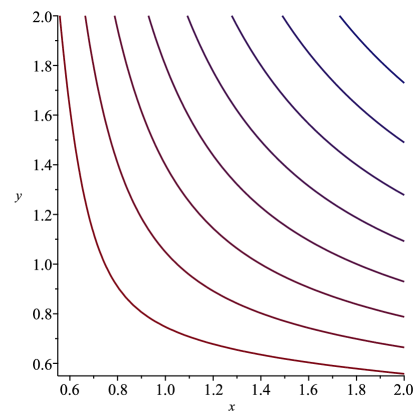
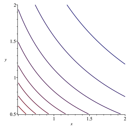
Figure 1: One loop amplitudes $1$ (left) and $2$ (right) for $S$.

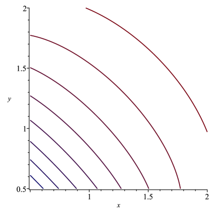
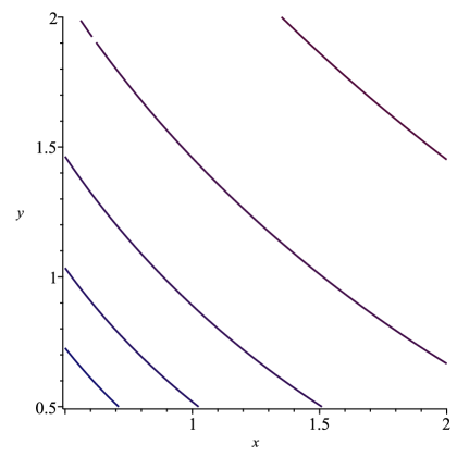
Figure 2: One loop amplitudes $1$ (left) and $2$ (right) for $V$.

For each of the other operators the expressions for the amplitudes are formally similar to (3.1) but larger. To assist with appreciating the structure of amplitudes for these other cases we have made similar contour plots for the same gauge, colour and flavour parameters as Figure 1 for the first two Lorentz channels. These are given in Figures 2, 3, 4 and 5. The behaviour of the results for $V$ and $T$ are similar in form. Recalling that channel $1$ for $S$, $V$ and $T$ contains an $O(1)$ term, but for the operator $W_{2}$ it is channel $2$, we see a larger variation over the domain we have chosen for these channels compared with the others. Though there is an exception for $T$ which is a reflection that in this case channel $2$ corresponds to a different partition of the $\Gamma_{(n)}$-matrices. For $\partial W_{2}$ we have plotted channel $3$ rather than $2$ since the latter is equivalent to the graph of channel $1$. This is because the operator $\partial W_{2}$ is a total derivative and this derivative introduces this symmetry. Moreover the plots for channel $1$ of $V$ and $\partial W_{2}$ are equivalent for similar reasons.

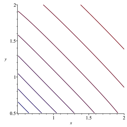
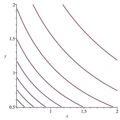
Figure 3: One loop amplitudes $1$ (left) and $2$ (right) for $T$.

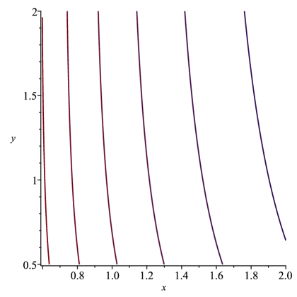
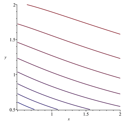
Figure 4: One loop amplitudes $1$ (left) and $2$ (right) for $W_{2}$.

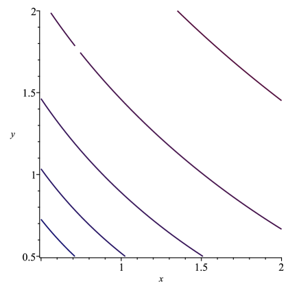
Figure 5: One loop amplitudes $1$ (left) and $3$ (right) for $\partial W_{2}$.

One aspect of our calculation which we have checked is the generalization of the relations between amplitudes given in [21, 22] are satisfied. By this we mean that in the original Green’s function one can interchange the external quark and antiquark legs which implies that several of the amplitudes in the Lorentz decomposition are related. For the general off-shell cases this means that the momenta $p$ and $q$ have to be swapped in the explicit expressions. For completeness we note that the relations are

$$\Sigma^{V}_{(2)}(p,q)~{}=~{}\Sigma^{V}_{(5)}(q,p)~{}~{}~{},~{}~{}~{}\Sigma^{V}_{(3)}(p,q)~{}=~{}\Sigma^{V}_{(4)}(q,p)$$ (3.2)

for the vector operator while

$$\Sigma^{T}_{(3)}(p,q)~{}=~{}\Sigma^{T}_{(6)}(q,p)~{}~{}~{},~{}~{}~{}\Sigma^{T}_{(4)}(p,q)~{}=~{}\Sigma^{T}_{(5)}(q,p)$$ (3.3)

are the corresponding ones for the tensor case. In the $W_{2}$ sector due to the asymmetry in the definition of the operator $W_{2}$ itself there are only symmetry relations for the $\partial W_{2}$ operator. These are

$$\Sigma^{\partial W_{2}}_{(1)}(p,q) = \Sigma^{\partial W_{2}}_{(2)}(q,p)~{}~{}~{},~{}~{}~{}\Sigma^{\partial W_{2}}_{(3)}(p,q)~{}=~{}\Sigma^{\partial W_{2}}_{(8)}(q,p)~{}~{},~{}~{}\Sigma^{\partial W_{2}}_{(4)}(p,q)~{}=~{}\Sigma^{\partial W_{2}}_{(7)}(q,p)$$

$$\Sigma^{\partial W_{2}}_{(5)}(p,q) = \Sigma^{\partial W_{2}}_{(6)}(q,p)~{}~{},~{}~{}\Sigma^{\partial W_{2}}_{(9)}(p,q)~{}=~{}\Sigma^{\partial W_{2}}_{(10)}(q,p)~{}.$$ (3.4)

In the case of each operator the order of the momenta arguments in the amplitude of the right hand side have been swapped. We have verified that each of the above relations for the respective operators hold to two loops for all $x$ and $y$. As a final check on our results we have taken the limits back to various results which are already known, [21, 22].

4 Discussion.

The computation of the Green’s function (2.6) which we have carried out here for the operators of (2.1) in the most general off-shell momentum configuration completes our programme to provide their full structure to two loops. With the provision of different momentum values for the external quark fields of (2.6) it should be possible to examine new aspects of the dynamics of the partons of the proton for problems of current interest. We note again that that the lattice evaluation of the pressure inside the proton, [20], would be one physical quantity of distinct interest given the potential to refine the comparison with the original experimental results of [19] further. That aside there are other uses for our results. For instance, the parton distribution functions have been considered on the lattice in, for example, [48, 49, 50, 51, 52]. Again the greater freedom to measure the Wilson operator Green’s function in a larger set of momenta choices should assist with improving our knowledge of the deeper structure of the proton. The subsequent stage to our programme will be to extend to the next loop order. This is not a trivial task for the general momentum configuration. It would require the expressions of the master integrals analogous to the two loop ones of [28, 29, 30, 31]. While progress to achieve this has been made in recent years, [53], with the provision of the algorithm to determine the master integrals the explicit functions are not yet known. That is the next stage in the programme.

Acknowledgements. This work was supported by a DFG Mercator Fellowship. The author thanks R. Horsley and P.E.L. Rakow for encouragement and valuable discussions as well as the Mathematical Physics Group at Humboldt University, Berlin for its hospitality where this work was initiated.

Appendix A Tensor bases and operator projection matrices.

In this appendix we record the basis tensors for the decomposition of each Green’s functions together with the elements of each projection matrix. While each is similar to their counterparts in previous momentum configurations, [21, 22], there are several differences in the general case where $x$ and $y$ are not restricted. For the scalar quark operator there are two tensors when there are two independent external momenta which are

$${\cal P}^{S}_{(1)}(p,q)~{}=~{}\Gamma_{(0)}~{}~{}~{},~{}~{}~{}{\cal P}^{S}_{(2)}(p,q)~{}=~{}\frac{1}{\mu^{2}}\Gamma_{(2)}^{pq}~{}.$$ (A.1)

In this and the other bases the scale $\mu$ will appear in several elements to ensure each has the same dimension. It also means that the elements of each projection matrix have the same dimension. As the scalar operator basis involves different elements of the generalized $\gamma$-matrices then the projection matrix is diagonal due to (2.12) giving

$${\cal M}^{S}~{}=~{}\frac{1}{4\Delta_{G}}\left(\begin{array}[]{cc}\Delta_{G}&0\\ 0&4\\ \end{array}\right)~{}.$$ (A.2)

There is a similar partition for the remaining projection matrices which are larger.

For the vector case there are six basis elements defined as

$${\cal P}^{V}_{(1)\mu}(p,q) = \gamma_{\mu}~{}~{}~{},~{}~{}~{}{\cal P}^{V}_{(2)\mu}(p,q)~{}=~{}\frac{{p}^{\mu}p\!\!\!/}{\mu^{2}}~{}~{}~{},~{}~{}~{}{\cal P}^{V}_{(3)\mu}(p,q)~{}=~{}\frac{{p}_{\mu}q\!\!\!/}{\mu^{2}}~{},$$

$${\cal P}^{V}_{(4)\mu}(p,q) = \frac{{q}_{\mu}p\!\!\!/}{\mu^{2}}~{}~{}~{},~{}~{}~{}{\cal P}^{V}_{(5)\mu}(p,q)~{}=~{}\frac{{q}_{\mu}q\!\!\!/}{\mu^{2}}~{}~{}~{},~{}~{}~{}{\cal P}^{V}_{(6)\mu}(p,q)~{}=~{}\frac{1}{\mu^{2}}\Gamma_{(3)\,\mu pq}$$ (A.3)

where the final one will form a unit partition. However as the projection matrix is now $6$ $\times$ $6$ but symmetric we will only list those non-zero elements of the upper triangle. Defining

$${\cal M}^{V}~{}=~{}\frac{1}{4[d-2]\Delta_{G}^{2}}\tilde{\cal M}^{V}$$ (A.4)

in order to extract the overall common factor we then have

$$\tilde{\cal M}^{V}_{11} = [x^{2}-2xy-2x+y^{2}-2y+1]^{2}~{}~{},~{}~{}\tilde{\cal M}^{V}_{12}~{}=~{}-~{}4[(y-1)^{2}+x^{2}-2(y+1)x]y$$

$$\tilde{\cal M}^{V}_{13} = -~{}2[x^{2}-2xy-2x+y^{2}-2y+1][x+y-1]$$

$$\tilde{\cal M}^{V}_{14} = -~{}2[x^{2}-2xy-2x+y^{2}-2y+1][x+y-1]$$

$$\tilde{\cal M}^{V}_{15} = -~{}4[(y-1)^{2}+x^{2}-2(y+1)x]x~{}~{},~{}~{}\tilde{\cal M}^{V}_{22}~{}=~{}16[d-1]y^{2}$$

$$\tilde{\cal M}^{V}_{23} = 8[d-1][x+y-1]y~{}~{},~{}~{}\tilde{\cal M}^{V}_{24}~{}=~{}8[d-1][x+y-1]y$$

$$\tilde{\cal M}^{V}_{25} = 4[dx^{2}+2dxy-2dx+dy^{2}-2dy+d-2x^{2}+4x-2y^{2}+4y-2]$$

$$\tilde{\cal M}^{V}_{33} = 4[4dxy+x^{2}-6xy-2x+y^{2}-2y+1]~{}~{},~{}~{}\tilde{\cal M}^{V}_{34}~{}=~{}4[d-1][x+y-1]^{2}$$

$$\tilde{\cal M}^{V}_{35} = 8[y-1+x][d-1]x~{}~{},~{}~{}\tilde{\cal M}^{V}_{44}~{}=~{}4[4dxy+x^{2}-6xy-2x+y^{2}-2y+1]$$

$$\tilde{\cal M}^{V}_{45} = 8[y-1+x][d-1]x~{}~{},~{}~{}\tilde{\cal M}^{V}_{55}~{}=~{}16[d-1]x^{2}$$

$$\tilde{\cal M}^{V}_{66} = 4[(y-1)^{2}+x^{2}-2(y+1)x]$$ (A.5)

where we have not listed the zero elements outside the $\Gamma_{(1)}$ and $\Gamma_{(3)}$ partitions.

Following [21, 22] our basis for the tensor operator is

$${\cal P}^{T}_{(1)\mu\nu}(p,q) = \Gamma_{(2)\,\mu\nu}~{}~{}~{},~{}~{}~{}{\cal P}^{T}_{(2)\mu\nu}(p,q)~{}=~{}\frac{1}{\mu^{2}}\left[p_{\mu}q_{\nu}-p_{\nu}q_{\mu}\right]\Gamma_{(0)}~{},$$

$${\cal P}^{T}_{(3)\mu\nu}(p,q) = \frac{1}{\mu^{2}}\left[\Gamma_{(2)\,\mu p}p_{\nu}-\Gamma_{(2)\,\nu p}p_{\mu}\right]~{}~{}~{},~{}~{}~{}{\cal P}^{T}_{(4)\mu\nu}(p,q)~{}=~{}\frac{1}{\mu^{2}}\left[\Gamma_{(2)\,\mu p}q_{\nu}-\Gamma_{(2)\,\nu p}q_{\mu}\right]~{},$$

$${\cal P}^{T}_{(5)\mu\nu}(p,q) = \frac{1}{\mu^{2}}\left[\Gamma_{(2)\,\mu q}p_{\nu}-\Gamma_{(2)\,\nu q}p_{\mu}\right]~{}~{}~{},~{}~{}~{}{\cal P}^{T}_{(6)\mu\nu}(p,q)~{}=~{}\frac{1}{\mu^{2}}\left[\Gamma_{(2)\,\mu q}q_{\nu}-\Gamma_{(2)\,\nu q}q_{\mu}\right]~{},$$

$${\cal P}^{T}_{(7)\mu\nu}(p,q) = \frac{1}{\mu^{4}}\left[\Gamma_{(2)\,pq}p_{\mu}q_{\nu}-\Gamma_{(2)\,pq}p_{\nu}q_{\mu}\right]~{}~{}~{},~{}~{}~{}{\cal P}^{T}_{(8)\mu\nu}(p,q)~{}=~{}\frac{1}{\mu^{2}}\Gamma_{(4)\,\mu\nu pq}~{}.$$ (A.6)

To record the elements of the projection matrix we define the factorized matrix ${\cal M}^{T}$ and set

$${\cal M}^{T}~{}=~{}\frac{1}{4[d-2][d-3]\Delta_{G}^{2}}\tilde{\cal M}^{T}~{}.$$ (A.7)

Then

$$\tilde{\cal M}^{T}_{11} = -~{}[x^{2}-2xy-2x+y^{2}-2y+1]^{2}~{}~{},~{}~{}\tilde{\cal M}^{T}_{12}~{}=~{}0$$

$$\tilde{\cal M}^{T}_{13} = 4[(y-1)^{2}+x^{2}-2(y+1)x]y~{}~{},~{}~{}\tilde{\cal M}^{T}_{14}~{}=~{}2[x^{2}-2xy-2x+y^{2}-2y+1][x+y-1]$$

$$\tilde{\cal M}^{T}_{15} = 2[x^{2}-2xy-2x+y^{2}-2y+1][x+y-1]~{}~{},~{}~{}\tilde{\cal M}^{T}_{16}~{}=~{}4[(y-1)^{2}+x^{2}-2(y+1)x]x$$

$$\tilde{\cal M}^{T}_{17} = 4[(y-1)^{2}+x^{2}-2(y+1)x]$$

$$\tilde{\cal M}^{T}_{22} = -~{}2[(y-1)^{2}+x^{2}-2(y+1)x][d-2][d-3]$$

$$\tilde{\cal M}^{T}_{23} = \tilde{\cal M}^{T}_{24}~{}=~{}\tilde{\cal M}^{T}_{25}~{}=~{}\tilde{\cal M}^{T}_{26}~{}=~{}\tilde{\cal M}^{T}_{27}~{}=~{}0~{}~{},~{}~{}\tilde{\cal M}^{T}_{33}~{}=~{}-~{}8[d-1]y^{2}$$

$$\tilde{\cal M}^{T}_{34} = -~{}4[d-1][x+y-1]y~{}~{},~{}~{}\tilde{\cal M}^{T}_{35}~{}=~{}-~{}4[d-1][x+y-1]y$$

$$\tilde{\cal M}^{T}_{36} = -~{}2[dx^{2}+2dxy-2dx+dy^{2}-2dy+d-3x^{2}+2xy+6x-3y^{2}+6y-3]$$

$$\tilde{\cal M}^{T}_{37} = -~{}8[d-1]y~{}~{},~{}~{}\tilde{\cal M}^{T}_{44}~{}=~{}-~{}4[2dxy+x^{2}-4xy-2x+y^{2}-2y+1]$$

$$\tilde{\cal M}^{T}_{45} = -~{}2[d-1][x+y-1]^{2}~{}~{},~{}~{}\tilde{\cal M}^{T}_{46}~{}=~{}-~{}4[y-1+x][d-1]x$$

$$\tilde{\cal M}^{T}_{47} = -~{}4[y-1+x][d-1]~{}~{},~{}~{}\tilde{\cal M}^{T}_{55}~{}=~{}-~{}4[2dxy+x^{2}-4xy-2x+y^{2}-2y+1]$$

$$\tilde{\cal M}^{T}_{56} = -~{}4[y-1+x][d-1]x~{}~{},~{}~{}\tilde{\cal M}^{T}_{57}~{}=~{}-~{}4[y-1+x][d-1]~{}~{},~{}~{}\tilde{\cal M}^{T}_{66}~{}=~{}-~{}8[d-1]x^{2}$$

$$\tilde{\cal M}^{T}_{67} = -~{}8[d-1]x~{}~{},~{}~{}\tilde{\cal M}^{T}_{77}~{}=~{}-~{}8[d-1][d-2]$$

$$\tilde{\cal M}^{T}_{88} = -~{}4[(y-1)^{2}+x^{2}-2(y+1)x]$$ (A.8)

are the upper triangle entries in the symmetric matrix.

The situation for the final operator $W_{2}$ is slightly different from the previous ones. In this we have chosen to define the basis in such a way that each Lorentz tensor is symmetric and traceless. While there is no a priori reason for doing so it results in some of our basis elements having $x$ and $y$ dependence unlike the derivative free operators. So the basis tensors formally differ from those of [21, 22]. However they equate to the latter in the respective limits. Our choice here is

$${\cal P}^{W_{2}}_{(1)\mu\nu}(p,q) = \gamma_{\mu}p_{\nu}+\gamma_{\nu}p_{\mu}-\frac{2}{d}p\!\!\!/\eta_{\mu\nu}~{}~{},~{}~{}{\cal P}^{W_{2}}_{(2)\mu\nu}(p,q)~{}=~{}\gamma_{\mu}q_{\nu}+\gamma_{\nu}q_{\mu}-\frac{2}{d}q\!\!\!/\eta_{\mu\nu}$$

$${\cal P}^{W_{2}}_{(3)\mu\nu}(p,q) = p\!\!\!/\left[\frac{1}{\mu^{2}}p_{\mu}p_{\nu}+\frac{x}{d}\eta_{\mu\nu}\right]~{},~{}{\cal P}^{W_{2}}_{(4)\mu\nu}(p,q)~{}=~{}p\!\!\!/\left[\frac{1}{\mu^{2}}p_{\mu}q_{\nu}+\frac{1}{\mu^{2}}q_{\mu}p_{\nu}+\frac{[1-x-y]}{d}\eta_{\mu\nu}\right]$$

$${\cal P}^{W_{2}}_{(5)\mu\nu}(p,q) = p\!\!\!/\left[\frac{1}{\mu^{2}}q_{\mu}q_{\nu}+\frac{y}{d}\eta_{\mu\nu}\right]~{},~{}{\cal P}^{W_{2}}_{(6)\mu\nu}(p,q)~{}=~{}q\!\!\!/\left[\frac{1}{\mu^{2}}p_{\mu}p_{\nu}+\frac{x}{d}\eta_{\mu\nu}\right]$$

$${\cal P}^{W_{2}}_{(7)\mu\nu}(p,q) = q\!\!\!/\left[\frac{1}{\mu^{2}}p_{\mu}q_{\nu}+\frac{1}{\mu^{2}}q_{\mu}p_{\nu}+\frac{[1-x-y]}{d}\eta_{\mu\nu}\right]~{},~{}{\cal P}^{W_{2}}_{(8)\mu\nu}(p,q)~{}=~{}q\!\!\!/\left[\frac{1}{\mu^{2}}q_{\mu}q_{\nu}+\frac{y}{d}\eta_{\mu\nu}\right]$$

$${\cal P}^{W_{2}}_{(9)\mu\nu}(p,q) = \frac{1}{\mu^{2}}\left[\Gamma_{(3)\,\mu pq}p_{\nu}+\Gamma_{(3)\,\nu pq}p_{\mu}\right]~{},~{}{\cal P}^{W_{2}}_{(10)\mu\nu}(p,q)~{}=~{}\frac{1}{\mu^{2}}\left[\Gamma_{(3)\,\mu pq}q_{\nu}+\Gamma_{(3)\,\nu pq}q_{\mu}\right]~{}.$$ (A.9)

This partitions the projection matrix into an $8$ $\times$ $8$ sub-matrix for the $\Gamma_{(1)}$-matrices and $2$ $\times$ $2$ for the $\Gamma_{(3)}$ sector. Defining

$${\cal M}^{W_{2}}~{}=~{}\frac{1}{4[d-2]^{2}\Delta_{G}^{3}\mu^{2}}\tilde{\cal M}^{W_{2}}$$ (A.10)

where the factor includes $\mu^{2}$ since the elements of the tensor basis each have an odd number of external momenta. The non-zero elements of the upper triangle of each sub-matrix of the two symmetric partitions of $\tilde{\cal M}^{W_{2}}$ are

$$\tilde{\cal M}^{W_{2}}_{11} = 2[d-2][x^{2}-2xy-2x+y^{2}-2y+1]^{2}y$$

$$\tilde{\cal M}^{W_{2}}_{12} = [d-2][x^{2}-2xy-2x+y^{2}-2y+1]^{2}[x+y-1]$$

$$\tilde{\cal M}^{W_{2}}_{13} = -~{}16[[y-1]^{2}+x^{2}-2[y+1]x][d-2]y^{2}$$

$$\tilde{\cal M}^{W_{2}}_{14} = -~{}8[d-2][x^{2}-2xy-2x+y^{2}-2y+1][x+y-1]y$$

$$\tilde{\cal M}^{W_{2}}_{15} = -~{}4[d-2][x^{2}-2xy-2x+y^{2}-2y+1][x+y-1]^{2}$$

$$\tilde{\cal M}^{W_{2}}_{16} = -~{}8[d-2][x^{2}-2xy-2x+y^{2}-2y+1][x+y-1]y$$

$$\tilde{\cal M}^{W_{2}}_{17} = -~{}2[d-2][x^{2}+6xy-2x+y^{2}-2y+1][x^{2}-2xy-2x+y^{2}-2y+1]$$

$$\tilde{\cal M}^{W_{2}}_{18} = -~{}8[d-2][x^{2}-2xy-2x+y^{2}-2y+1][x+y-1]x$$

$$\tilde{\cal M}^{W_{2}}_{22} = 2[d-2][x^{2}-2xy-2x+y^{2}-2y+1]^{2}x$$

$$\tilde{\cal M}^{W_{2}}_{23} = -~{}8[d-2][x^{2}-2xy-2x+y^{2}-2y+1][x+y-1]y$$

$$\tilde{\cal M}^{W_{2}}_{24} = -~{}2[d-2][x^{2}+6xy-2x+y^{2}-2y+1][x^{2}-2xy-2x+y^{2}-2y+1]$$

$$\tilde{\cal M}^{W_{2}}_{25} = -~{}8[d-2][x^{2}-2xy-2x+y^{2}-2y+1][x+y-1]x$$

$$\tilde{\cal M}^{W_{2}}_{26} = -~{}4[d-2][x^{2}-2xy-2x+y^{2}-2y+1][x+y-1]^{2}$$

$$\tilde{\cal M}^{W_{2}}_{27} = -~{}8[d-2][x^{2}-2xy-2x+y^{2}-2y+1][x+y-1]x$$

$$\tilde{\cal M}^{W_{2}}_{28} = -~{}16[[y-1]^{2}+x^{2}-2[y+1]x][d-2]x^{2}~{}~{},~{}~{}\tilde{\cal M}^{W_{2}}_{33}~{}=~{}64[d+1][d-2]y^{3}$$

$$\tilde{\cal M}^{W_{2}}_{34} = 32[d+1][d-2][x+y-1]y^{2}$$

$$\tilde{\cal M}^{W_{2}}_{35} = 16[dx^{2}+2dxy-2dx+dy^{2}-2dy+d+4xy][d-2]y$$

$$\tilde{\cal M}^{W_{2}}_{36} = 32[d+1][d-2][x+y-1]y^{2}$$

$$\tilde{\cal M}^{W_{2}}_{37} = 16[dx^{2}+2dxy-2dx+dy^{2}-2dy+d+4xy][d-2]y$$

$$\tilde{\cal M}^{W_{2}}_{38} = 8[d(x+y-1)^{2}+8xy+4x-2y^{2}+4y-2][d-2][x+y-1]$$

$$\tilde{\cal M}^{W_{2}}_{44} = 8[dx^{2}+6dxy-2dx+dy^{2}-2dy+d+3x^{2}+2xy-6x+3y^{2}-6y+3][d-2]y$$

$$\tilde{\cal M}^{W_{2}}_{45} = 8[4dxy+x^{2}+2xy-2x+y^{2}-2y+1][d-2][x+y-1]$$

$$\tilde{\cal M}^{W_{2}}_{46} = 16[d+1][d-2][x+y-1]^{2}y$$

$$\tilde{\cal M}^{W_{2}}_{47} = 4[d+1][d-2][x^{2}+6xy-2x+y^{2}-2y+1][x+y-1]$$

$$\tilde{\cal M}^{W_{2}}_{48} = 16[dx^{2}+2dxy-2dx+dy^{2}-2dy+d+4xy][d-2]x$$

$$\tilde{\cal M}^{W_{2}}_{55} = 32[2dxy+x^{2}-2x+y^{2}-2y+1][d-2]x$$

$$\tilde{\cal M}^{W_{2}}_{56} = 8[dx^{2}+2dxy-2dx+dy^{2}-2dy+d+4xy][d-2][x+y-1]$$

$$\tilde{\cal M}^{W_{2}}_{57} = 16[d+1][d-2][x+y-1]^{2}x~{}~{},~{}~{}\tilde{\cal M}^{W_{2}}_{58}~{}=~{}32[d+1][d-2][x+y-1]x^{2}$$

$$\tilde{\cal M}^{W_{2}}_{66} = 32[2dxy+x^{2}-2x+y^{2}-2y+1][d-2]y$$

$$\tilde{\cal M}^{W_{2}}_{67} = 8[4dxy+x^{2}+2xy-2x+y^{2}-2y+1][d-2][x+y-1]$$

$$\tilde{\cal M}^{W_{2}}_{68} = 16[dx^{2}+2dxy-2dx+dy^{2}-2dy+d+4xy][d-2]x$$

$$\tilde{\cal M}^{W_{2}}_{77} = 8[dx^{2}+6dxy-2dx+dy^{2}-2dy+d+3x^{2}+2xy-6x+3y^{2}-6y+3][d-2]x$$

$$\tilde{\cal M}^{W_{2}}_{78} = 32[d+1][d-2][x+y-1]x^{2}~{}~{},~{}~{}\tilde{\cal M}^{W_{2}}_{88}~{}=~{}64[d+1][d-2]x^{3}$$

$$\tilde{\cal M}^{W_{2}}_{99} = 8\Delta_{G}^{2}[d-2]y~{}~{},~{}~{}\tilde{\cal M}^{W_{2}}_{910}~{}=~{}4[d-2]\Delta_{G}[x+y-1]$$

$$\tilde{\cal M}^{W_{2}}_{1010} = 8\Delta_{G}[d-2]x~{}.$$ (A.11)

Appendix B Basic integrals.

In the final expressions for the operator Green’s functions several core functions arise which are combinations of the polylogarithm function $\mbox{Li}_{n}(z)$. We record them here for completeness. The main function at one loop is

$$\Phi_{1}(x,y)~{}=~{}\frac{1}{\lambda}\left[2\mbox{Li}_{2}(-\rho x)+2\mbox{Li}_{2}(-\rho y)+\ln\left(\frac{y}{x}\right)\ln\left(\frac{(1+\rho y)}{(1+\rho x)}\right)+\ln(\rho x)\ln(\rho y)+\frac{\pi^{2}}{3}\right]$$ (B.1)

where $\lambda(x,y)$ and $\rho(x,y)$ are given by, [29, 30],

$$\lambda(x,y)~{}=~{}\sqrt{\Delta_{G}}~{}~{}~{},~{}~{}~{}\rho(x,y)~{}=~{}\frac{2}{[1-x-y+\lambda(x,y)]}$$ (B.2)

and throughout this section $x$ and $y$ are variables in general not to be confused with the kinematic ones of (2.8). However the triangle graph where $\Phi_{1}(x,y)$ arises has an $O(\epsilon)$ correction which cannot be neglected a priori for the two loop evaluation. It is given by, [29, 30],

$$\Psi_{1}(x,y) = -~{}\frac{1}{\lambda}\left[4\mbox{Li}_{3}\left(-\frac{\rho x(1+\rho y)}{(1-\rho^{2}xy)}\right)+4\mbox{Li}_{3}\left(-\frac{\rho y(1+\rho x)}{(1-\rho^{2}xy)}\right)-4\mbox{Li}_{3}\left(-\frac{xy\rho^{2}}{(1-\rho^{2}xy)}\right)\right.$$ (B.3)

$$\left.~{}~{}~{}~{}~{}~{}~{}+2\mbox{Li}_{3}\left(\frac{x\rho(1+\rho y)}{(1+\rho x)}\right)+2\mbox{Li}_{3}\left(\frac{y\rho(1+\rho x)}{(1+\rho y)}\right)-2\mbox{Li}_{3}(\rho^{2}xy)-2\zeta_{3}\right.$$

$$\left.~{}~{}~{}~{}~{}~{}~{}-2\ln(y)\mbox{Li}_{2}\left(\frac{x\rho(1+\rho y)}{(1+\rho x)}\right)-2\ln(x)\mbox{Li}_{2}\left(\frac{y\rho(1+\rho x)}{(1+\rho y)}\right)-\frac{2}{3}\ln^{3}\left(1-\rho^{2}xy\right)\right.$$

$$\left.~{}~{}~{}~{}~{}~{}~{}+\frac{2}{3}\ln^{3}\left(1+\rho x\right)+\frac{2}{3}\ln^{3}\left(1+\rho y\right)+2\ln(\rho)\ln^{2}\left(1-\rho^{2}xy\right)\right.$$

$$\left.~{}~{}~{}~{}~{}~{}~{}-2\ln(1-\rho^{2}xy)\left[\ln(\rho x)\ln(\rho y)+\ln\left(\frac{y}{x}\right)\ln\left(\frac{(1+\rho y)}{(1+\rho x)}\right)\right.\right.$$

$$\left.\left.~{}~{}~{}~{}~{}~{}~{}~{}~{}~{}~{}~{}~{}~{}~{}~{}~{}~{}~{}~{}~{}~{}~{}~{}~{}~{}~{}~{}~{}~{}+2\ln(1+\rho x)\ln(1+\rho y)+\frac{\pi^{2}}{3}\right]\right.$$

$$\left.~{}~{}~{}~{}~{}~{}~{}+\frac{1}{2}\ln\left(xy\rho^{2}\right)\left[\ln(\rho x)\ln(\rho y)+\ln\left(\frac{y}{x}\right)\ln\left(\frac{(1+\rho y)}{(1+\rho x)}\right)-\ln^{2}\left(\frac{(1+\rho x)}{(1+\rho y)}\right)\right.\right.$$

$$\left.\left.~{}~{}~{}~{}~{}~{}~{}~{}~{}~{}~{}~{}~{}~{}~{}~{}~{}~{}~{}~{}~{}~{}~{}~{}~{}~{}~{}+\frac{2\pi^{2}}{3}\right]\right]~{}.$$

At the next loop order there are two key functions in the two loop master integrals. These are, [28, 29],

$$\Phi_{2}(x,y) = \frac{1}{\lambda}\left[6\mbox{Li}_{4}(-\rho x)+6\mbox{Li}_{4}(-\rho y)+3\ln\left(\frac{y}{x}\right)\left[\mbox{Li}_{3}(-\rho x)-\mbox{Li}_{3}(-\rho y)\right]\right.$$ (B.4)

$$\left.~{}~{}~{}+\frac{1}{2}\ln^{2}\left(\frac{y}{x}\right)\left[\mbox{Li}_{2}(-\rho x)+\mbox{Li}_{2}(-\rho y)\right]+\frac{1}{4}\ln^{2}(\rho x)\ln^{2}(\rho y)\right.$$

$$\left.~{}~{}~{}+\frac{\pi^{2}}{2}\ln(\rho x)\ln(\rho y)+\frac{\pi^{2}}{12}\ln^{2}\left(\frac{y}{x}\right)+\frac{7\pi^{4}}{60}\right]$$

and

$$\Omega_{2}(x,y) = 6\mbox{Li}_{3}(-\rho x)+6\mbox{Li}_{3}(-\rho y)+3\ln\left(\frac{y}{x}\right)\left[\mbox{Li}_{2}(-\rho x)-\mbox{Li}_{2}(-\rho y)\right]$$ (B.5)

$$-~{}\frac{1}{2}\ln^{2}\left(\frac{y}{x}\right)\left[\ln(1+\rho x)+\ln(1+\rho y)\right]$$

$$+~{}\frac{1}{2}\left[\pi^{2}+\ln(\rho x)\ln(\rho y)\right]\left[\ln(\rho x)+\ln(\rho y)\right]~{}.$$

These functions are related to cyclotomic polylogarithms, [54].