Approximate Inference Turns Deep Networks into Gaussian Processes

Mohammad Emtiyaz Khan
RIKEN Center for AI Project
Tokyo, Japan
emtiyaz.khan@riken.jp
&Alexander Immer*
EPFL
Lausanne, Switzerland
alexander.immer@epfl.ch
Ehsan Abedi*11footnotemark: 1
EPFL
Lausanne, Switzerland
ehsan.abedi@epfl.ch
&Maciej Korzepa*11footnotemark: 1
Technical University of Denmark
Kgs. Lyngby, Denmark
mjko@dtu.dk
Equal contribution. *This work is performed during an internship at the RIKEN Center for AI project.
Abstract

Deep neural networks (DNN) and Gaussian processes (GP) are two powerful models with several theoretical connections relating them, but the relationship between their training methods is not well understood. In this paper, we show that certain Gaussian posterior approximations for Bayesian DNNs are equivalent to GP posteriors. This enables us to relate solutions and iterations of a deep-learning algorithm to GP inference. As a result, we can obtain a GP kernel and a nonlinear feature map while training a DNN. Surprisingly, the resulting kernel is the neural tangent kernel. We show kernels obtained on real datasets and demonstrate the use of the GP marginal likelihood to tune hyperparameters of DNNs. Our work aims to facilitate further research on combining DNNs and GPs in practical settings.

1 Introduction

Deep neural networks (DNN) and Gaussian processes (GP) models are both powerful models with complementary strengths and weaknesses. DNNs achieve state-of-the-art results on many real-world problems providing scalable end-to-end learning, but they can overfit on small datasets and be overconfident. In contrast, GPs are suitable for small datasets and compute confidence estimates, but they are not scalable and choosing a good kernel in practice is challenging [3]. Combining their strengths to solve real-world problems is an important problem.

Theoretically, the two models are closely related to each other. Previous work has shown that as the width of a DNN increases to infinity, the DNN converges to a GP [4, 5, 13, 16, 22]. This relationship is surprising and gives us hope that a practical combination could be possible. Unfortunately, it is not clear how one can use such connections in practice, e.g., to perform fast inference in GPs by using training methods of DNNs, or to reduce overfitting in DNNs by using GP inference. We argue that, to solve such practical problems, we need the relationship not only between the models but also between their training procedures. The purpose of this paper is to provide such a theoretical relationship.

We present theoretical results aimed at connecting the training methods of deep learning and GP models. We show that the Gaussian posterior approximations for Bayesian DNNs, such as those obtained by Laplace approximation and variational inference (VI), are equivalent to posterior distributions of GP regression models. This result enables us to relate the solutions and iterations of a deep-learning algorithm to GP inference. See Fig. 1 for our approach called DNN2GP. In addition, we can obtain GP kernels and nonlinear feature maps while training a DNN (see Fig. 2). Surprisingly, a GP kernel we derive is equivalent to the recently proposed neural tangent kernel (NTK) [8].We present empirical results where we visualize the feature-map obtained on benchmark datasets such as MNIST and CIFAR, and demonstrate their use for DNN hyperparameter tuning. The code to reproduce our results is available at https://github.com/team-approx-bayes/dnn2gp. The work presented in this paper aims to facilitate further research on combining the strengths of DNNs and GPs in practical settings.

Refer to caption
Figure 1: A summary of our approach called DNN2GP in three steps.
Refer to caption
(a) 2D classification problem
Refer to caption
(b) GP kernel feature ϕ(𝐱)bold-italic-ϕ𝐱\mbox{$\mbox{$\boldsymbol{\phi}$}$}(\mbox{$\mbox{$\mathbf{x}$}$})
Refer to caption
(c) GP kernel
Refer to caption
(d) GP posterior mean
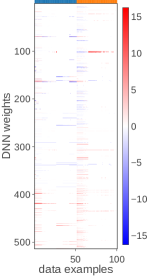
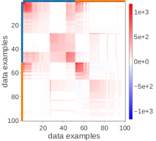
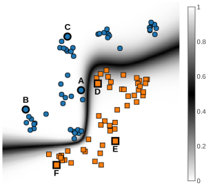
Figure 2: Fig. (a) shows a 2D binary-classification problem along with the predictive distribution of a DNN using 513 parameters. The corresponding feature and kernel matrices obtained using our approach are shown in (b) and (c), respectively (the two classes are grouped, and marked with blue and orange color along the axes). Fig. (d) shows the GP posterior mean where we see a clear separation between the two classes. Surprisingly, the border points A and D in (a) are also at the boundary in (d).

1.1 Related Work

The equivalence between infinitely-wide neural networks and GPs was originally discussed by Neal [16]. Subsequently, many works derived explicit expressions for the GP kernel corresponding to neural networks [4, 7, 16] and their deep variants [5, 6, 13, 18]. These works use a prior distribution on weights and derive kernels by averaging over the prior. Our work differs from these works in the fact that we use the posterior approximations to relate DNNs to GPs. Unlike these previous results, our results hold for DNNs of finite width.

A GP kernel we derive is equivalent to the recently proposed Neural Tangent Kernel (NTK) [8], which is obtained by using the Jacobian of the DNN outputs. For randomly initialized trajectories, as the DNN width goes to infinity, the NTK converges in probability to a deterministic kernel and remains asymptotically constant when training with gradient descent. Jacot et al. [8] motivate the NTK by using kernel gradient descent. Surprisingly, the NTK appears in our work with an entirely different approach where we consider approximations of the posterior distribution over weights. Due to connections to the NTK, we expect similar properties for our kernel. Our approach additionally shows that we can obtain other types of kernels by using different approximate inference methods.

In a recent work, Lee et al. [14] derive the mean and covariance function corresponding to the GP induced by the NTK. Unfortunately, the model does not correspond to inference in a GP model (see Section 2.3.1 in their paper). Our approach does not have this issue and we can express Gaussian posterior approximations on a Bayesian DNN as inference in a GP regression model.

2 Deep Neural Networks (DNNs) and Gaussian Processes (GPs)

The goal of this paper is to present a theoretical relationship between training methods of DNNs and GPs. DNNs are typically trained by minimizing an empirical loss between the data and the predictions. For example, in supervised learning with a dataset 𝒟:={(𝐱i,𝐲i)}i=1Nassign𝒟superscriptsubscriptsubscript𝐱𝑖subscript𝐲𝑖𝑖1𝑁\mbox{${\cal D}$}:=\{(\mbox{$\mbox{$\mathbf{x}$}$}_{i},\mbox{$\mbox{$\mathbf{y}$}$}_{i})\}_{i=1}^{N} of N𝑁N examples of input 𝐱iD\mbox{$\mbox{$\mathbf{x}$}$}_{i}\in{}^{D} and output 𝐲iK\mbox{$\mbox{$\mathbf{y}$}$}_{i}\in{}^{K}, we can minimize a loss of the following form:

¯(𝒟,𝐰):=i=1Ni(𝐰)+12δ𝐰𝐰, where i(𝐰):=(𝐲i,𝐟w(𝐱i)),formulae-sequenceassign¯𝒟𝐰superscriptsubscript𝑖1𝑁subscript𝑖𝐰12𝛿superscript𝐰top𝐰assign where subscript𝑖𝐰subscript𝐲𝑖subscript𝐟𝑤subscript𝐱𝑖\displaystyle\bar{\ell}(\mbox{${\cal D}$},\mbox{$\mbox{$\mathbf{w}$}$}):=\sum_{i=1}^{N}\ell_{i}(\mbox{$\mbox{$\mathbf{w}$}$})+\mbox{$\frac{1}{2}$}\delta\mbox{$\mbox{$\mathbf{w}$}$}^{\top}\mbox{$\mbox{$\mathbf{w}$}$},\quad\textrm{ where }\ell_{i}(\mbox{$\mbox{$\mathbf{w}$}$}):=\ell(\mbox{$\mbox{$\mathbf{y}$}$}_{i},\mbox{$\mbox{$\mathbf{f}$}$}_{w}(\mbox{$\mbox{$\mathbf{x}$}$}_{i})), (1)

where 𝐟w(𝐱)K\mbox{$\mbox{$\mathbf{f}$}$}_{w}(\mbox{$\mbox{$\mathbf{x}$}$})\in{}^{K} denotes the DNN outputs with weights 𝐰P\mbox{$\mbox{$\mathbf{w}$}$}\in{}^{P}, (𝐲,𝐟(𝐱))𝐲𝐟𝐱\ell(\mbox{$\mbox{$\mathbf{y}$}$},\mbox{$\mbox{$\mathbf{f}$}$}(\mbox{$\mbox{$\mathbf{x}$}$})) denotes a loss function between an output 𝐲𝐲\mathbf{y} and the function 𝐟(𝐱)𝐟𝐱\mbox{$\mbox{$\mathbf{f}$}$}(\mbox{$\mbox{$\mathbf{x}$}$}), and δ𝛿\delta is a small L2subscript𝐿2L_{2} regularizer.111We can assume that δ𝛿\delta is small enough that it does not affect the DNN’s generalization.. We assume the loss function to be twice differentiable and strictly convex in 𝐟𝐟\mathbf{f} (e.g., squared loss and cross-entropy loss). An attractive feature of DNNs is that they can be trained using stochastic-gradient (SG) methods [11]. Such methods scale well to large data settings.

GP models use an entirely different modeling approach which is based on directly modeling the functions rather than the parameters. For example, for regression problems with scalar outputs yisubscript𝑦𝑖absenty_{i}\in\real, consider the following linear basis-function model with a nonlinear feature-map ϕ(𝐱):DP\mbox{$\mbox{$\boldsymbol{\phi}$}$}(\mbox{$\mbox{$\mathbf{x}$}$}):{}^{D}\mapsto{}^{P}:

y𝑦\displaystyle y =ϕ(𝐱)𝐰+ϵ, with ϵ𝒩(0,σ2), and 𝐰𝒩(0,δ1𝐈P),formulae-sequenceabsentbold-italic-ϕsuperscript𝐱top𝐰italic-ϵformulae-sequencesimilar-to with italic-ϵ𝒩0superscript𝜎2similar-to and 𝐰𝒩0superscript𝛿1subscript𝐈𝑃\displaystyle=\mbox{$\mbox{$\boldsymbol{\phi}$}$}(\mbox{$\mbox{$\mathbf{x}$}$})^{\top}\mbox{$\mbox{$\mathbf{w}$}$}+\epsilon,\,\,\textrm{ with }\epsilon\sim\mbox{${\cal N}$}(0,\sigma^{2}),\,\,\textrm{ and }\mbox{$\mbox{$\mathbf{w}$}$}\sim\mbox{${\cal N}$}(0,\delta^{-1}\mbox{$\mbox{$\mathbf{I}$}$}_{P}), (2)

where 𝐈Psubscript𝐈𝑃\mbox{$\mbox{$\mathbf{I}$}$}_{P} is a P×P𝑃𝑃P\times P identity matrix and σ2superscript𝜎2\sigma^{2} is the output noise variance. Defining the function to be f(𝐱):=ϕ(𝐱)𝐰assign𝑓𝐱bold-italic-ϕsuperscript𝐱top𝐰f(\mbox{$\mbox{$\mathbf{x}$}$}):=\mbox{$\mbox{$\boldsymbol{\phi}$}$}(\mbox{$\mbox{$\mathbf{x}$}$})^{\top}\mbox{$\mbox{$\mathbf{w}$}$}, the predictive distribution p(f(𝐱)|𝐱,𝒟)𝑝conditional𝑓subscript𝐱subscript𝐱𝒟p(f(\mbox{$\mbox{$\mathbf{x}$}$}_{*})|\mbox{$\mbox{$\mathbf{x}$}$}_{*},\mbox{${\cal D}$}) at a new test input 𝐱subscript𝐱\mbox{$\mbox{$\mathbf{x}$}$}_{*} is equal to that of the following model directly defined with a GP prior over f(𝐱)𝑓𝐱f(\mbox{$\mbox{$\mathbf{x}$}$}) [23]:

y=f(𝐱)+ϵ, with f(𝐱)𝒢𝒫(0,κ(𝐱,𝐱)),formulae-sequence𝑦𝑓𝐱italic-ϵsimilar-to with 𝑓𝐱𝒢𝒫0𝜅𝐱superscript𝐱\displaystyle y=f(\mbox{$\mbox{$\mathbf{x}$}$})+\epsilon,\,\,\textrm{ with }f(\mbox{$\mbox{$\mathbf{x}$}$})\sim\mathcal{GP}\left(0,\kappa(\mbox{$\mbox{$\mathbf{x}$}$},\mbox{$\mbox{$\mathbf{x}$}$}^{\prime})\right), (3)

where κ(𝐱,𝐱):=𝔼[f(𝐱)f(𝐱)]=δ1ϕ(𝐱)ϕ(𝐱)assign𝜅𝐱superscript𝐱𝔼delimited-[]𝑓𝐱𝑓superscript𝐱superscript𝛿1bold-italic-ϕsuperscript𝐱topbold-italic-ϕsuperscript𝐱\kappa(\mbox{$\mbox{$\mathbf{x}$}$},\mbox{$\mbox{$\mathbf{x}$}$}^{\prime}):=\mathbb{E}[f(\mbox{$\mbox{$\mathbf{x}$}$})f(\mbox{$\mbox{$\mathbf{x}$}$}^{\prime})]=\delta^{-1}\mbox{$\mbox{$\boldsymbol{\phi}$}$}(\mbox{$\mbox{$\mathbf{x}$}$})^{\top}\mbox{$\mbox{$\boldsymbol{\phi}$}$}(\mbox{$\mbox{$\mathbf{x}$}$}^{\prime}) is the covariance function or kernel of the GP. The function-space model is more general in the sense that it can also deal with infinite-dimensional vector feature maps ϕ(𝐱)bold-italic-ϕ𝐱\mbox{$\mbox{$\boldsymbol{\phi}$}$}(\mbox{$\mbox{$\mathbf{x}$}$}), giving us a nonparametric model. This view has been used to show that as a DNN becomes infinitely wide it tends to a GP, by essentially showing that averaging over p(𝐰)𝑝𝐰p(\mbox{$\mbox{$\mathbf{w}$}$}) with the feature map induced by a DNN leads to a GP covariance function [16].

An attractive property of the function-space formulation as opposed to the weight-space formulation, such as (1), is that the posterior distribution has a closed-form expression. Another attractive property is that the posterior is usually unimodal, unlike the loss l¯(𝒟,𝐰)¯𝑙𝒟𝐰\bar{l}(\mbox{${\cal D}$},\mbox{$\mbox{$\mathbf{w}$}$}) which is typically nonconvex. Unfortunately, the computation of the posterior takes O(N3)𝑂superscript𝑁3O(N^{3}) which is infeasible for large datasets. GPs also require choosing a good kernel [23]. Unlike DNNs, inference in GPs remains much more difficult.

To summarize, despite the similarities between the two models, their training methods are fundamentally different. While DNNs employ stochastic optimization, GPs use closed-form updates. How can we relate these seemingly different training procedures in practical settings, e.g., without assuming infinite-width DNNs? In this paper, we provide an answer to this question. We derive theoretical results that relate the solutions and iterations of deep-learning algorithms to GP inference. We do so by first finding a Gaussian posterior approximation (Step A in Fig. 1), then use it to find a linear basis-function model (Step B in Fig. 1) and its corresponding GP (Step C in Fig. 1). We start in the next section with our first theoretical result.

3 Relating Minima of the Loss to GP Inference via Laplace Approximation

In this section, we present theoretical results relating minima of a deep-learning loss (1) to inference in GP models. A local minimizer 𝐰subscript𝐰\mbox{$\mbox{$\mathbf{w}$}$}_{*} of the loss (1) satisfies the following first-order and second-order conditions [17]: w¯(𝒟,𝐰)=0subscript𝑤¯𝒟subscript𝐰0\nabla_{w}\bar{\ell}(\mbox{${\cal D}$},\mbox{$\mbox{$\mathbf{w}$}$}_{*})=0 and ww2¯(𝒟,𝐰)0succeedssuperscriptsubscript𝑤𝑤2¯𝒟subscript𝐰0\nabla_{ww}^{2}\bar{\ell}(\mbox{${\cal D}$},\mbox{$\mbox{$\mathbf{w}$}$}_{*})\succ 0. Deep-learning optimizers, such as RMSprop and Adam, aim to find such minimizers, and our goal is to relate them to GP inference.

Step A (Laplace Approximation): To do so, we will use an approximate inference method called the Laplace approximation [1]. The minima of the loss (1) corresponds to a mode of the Bayesian model: p(𝒟,𝐰):=i=1Nei(𝐰)p(𝐰)assign𝑝𝒟𝐰superscriptsubscriptproduct𝑖1𝑁superscript𝑒subscript𝑖𝐰𝑝𝐰p(\mbox{${\cal D}$},\mbox{$\mbox{$\mathbf{w}$}$}):=\prod_{i=1}^{N}e^{-\ell_{i}(\mathbf{w})}p(\mbox{$\mbox{$\mathbf{w}$}$}) with prior distribution p(𝐰):=𝒩(𝐰|0,δ1𝐈P)assign𝑝𝐰𝒩conditional𝐰0superscript𝛿1subscript𝐈𝑃p(\mbox{$\mbox{$\mathbf{w}$}$}):=\mbox{${\cal N}$}(\mbox{$\mbox{$\mathbf{w}$}$}|0,\delta^{-1}\mbox{$\mbox{$\mathbf{I}$}$}_{P}), assuming that the posterior is well-defined. The posterior distribution p(𝐰|𝒟)=p(𝒟,𝐰)/p(𝒟)𝑝conditional𝐰𝒟𝑝𝒟𝐰𝑝𝒟p(\mbox{$\mbox{$\mathbf{w}$}$}|\mbox{${\cal D}$})=p(\mbox{${\cal D}$},\mbox{$\mbox{$\mathbf{w}$}$})/p(\mbox{${\cal D}$}) is usually computationally intractable and requires computationally-feasible approximation methods. The Laplace approximation uses the following Gaussian approximation for the posterior:

p(𝐰|𝒟)𝒩(𝐰|𝝁,𝚺), where 𝝁=𝐰 and 𝚺1=i=1Nww2i(𝐰)+δ𝐈P.formulae-sequence𝑝conditional𝐰𝒟𝒩conditional𝐰𝝁𝚺 where 𝝁subscript𝐰superscript and 𝚺1superscriptsubscript𝑖1𝑁superscriptsubscript𝑤𝑤2subscript𝑖subscript𝐰𝛿subscript𝐈𝑃\displaystyle p(\mbox{$\mbox{$\mathbf{w}$}$}|\mbox{${\cal D}$})\approx\mbox{${\cal N}$}(\mbox{$\mbox{$\mathbf{w}$}$}|\mbox{$\mbox{$\boldsymbol{\mu}$}$},\mbox{$\mbox{$\boldsymbol{\Sigma}$}$}),\textrm{ where }\mbox{$\mbox{$\boldsymbol{\mu}$}$}=\mbox{$\mbox{$\mathbf{w}$}$}_{*}\textrm{ and }\mbox{$\mbox{$\boldsymbol{\Sigma}$}$}^{-1}=\sum_{i=1}^{N}\nabla_{ww}^{2}\ell_{i}(\mbox{$\mbox{$\mathbf{w}$}$}_{*})+\delta\mbox{$\mbox{$\mathbf{I}$}$}_{P}. (4)

This approximation can be directly built using the solutions found by deep-learning optimizers.

Step B (Linear Model): The next step is to find a linear basis-function model whose posterior distribution is equal to the Gaussian approximation (4). We will now show that this is always possible whenever the gradient and Hessian of the loss222For notational convenience, we sometime use (𝐰)𝐰\ell(\mbox{$\mbox{$\mathbf{w}$}$}) to denote (𝐲,𝐟w(𝐱))𝐲subscript𝐟𝑤𝐱\ell(\mbox{$\mbox{$\mathbf{y}$}$},\mbox{$\mbox{$\mathbf{f}$}$}_{w}(\mbox{$\mbox{$\mathbf{x}$}$})). can be approximated as follows:

w(𝐰)ϕw(𝐱)𝐯w(𝐱,𝐲),ww2(𝐰)ϕw(𝐱)𝐃w(𝐱,𝐲)ϕw(𝐱),formulae-sequencesubscript𝑤𝐰subscriptbold-italic-ϕ𝑤𝐱subscript𝐯𝑤𝐱𝐲superscriptsubscript𝑤𝑤2𝐰subscriptbold-italic-ϕ𝑤𝐱subscript𝐃𝑤𝐱𝐲subscriptbold-italic-ϕ𝑤superscript𝐱top\displaystyle\nabla_{w}\ell(\mbox{$\mbox{$\mathbf{w}$}$})\approx\mbox{$\mbox{$\boldsymbol{\phi}$}$}_{w}(\mbox{$\mbox{$\mathbf{x}$}$})\mbox{$\mbox{$\mathbf{v}$}$}_{w}(\mbox{$\mbox{$\mathbf{x}$}$},\mbox{$\mbox{$\mathbf{y}$}$}),\quad\quad\nabla_{ww}^{2}\ell(\mbox{$\mbox{$\mathbf{w}$}$})\approx\mbox{$\mbox{$\boldsymbol{\phi}$}$}_{w}(\mbox{$\mbox{$\mathbf{x}$}$})\mbox{$\mbox{$\mathbf{D}$}$}_{w}(\mbox{$\mbox{$\mathbf{x}$}$},\mbox{$\mbox{$\mathbf{y}$}$})\mbox{$\mbox{$\boldsymbol{\phi}$}$}_{w}(\mbox{$\mbox{$\mathbf{x}$}$})^{\top}, (5)

where ϕw(𝐱)subscriptbold-italic-ϕ𝑤𝐱\mbox{$\mbox{$\boldsymbol{\phi}$}$}_{w}(\mbox{$\mbox{$\mathbf{x}$}$}) is a P×Q𝑃𝑄P\times Q feature matrix with Q𝑄Q as a positive integer, 𝐯w(𝐱,𝐲)subscript𝐯𝑤𝐱𝐲\mbox{$\mbox{$\mathbf{v}$}$}_{w}(\mbox{$\mbox{$\mathbf{x}$}$},\mbox{$\mbox{$\mathbf{y}$}$}) is a Q𝑄Q length vector, and 𝐃w(𝐱,𝐲)subscript𝐃𝑤𝐱𝐲\mbox{$\mbox{$\mathbf{D}$}$}_{w}(\mbox{$\mbox{$\mathbf{x}$}$},\mbox{$\mbox{$\mathbf{y}$}$}) is a Q×Q𝑄𝑄Q\times Q symmetric positive-definite matrix. We will now present results for a specific choice ϕw,𝐯wsubscriptbold-italic-ϕ𝑤subscript𝐯𝑤\mbox{$\mbox{$\boldsymbol{\phi}$}$}_{w},\mbox{$\mbox{$\mathbf{v}$}$}_{w}, and 𝐃wsubscript𝐃𝑤\mbox{$\mbox{$\mathbf{D}$}$}_{w}. Our proof trivially generalizes to arbitrary choices of these quantities.

For the loss of form (1), the gradient and Hessian take the following form [15, 17]:

w(𝐰)subscript𝑤𝐰\displaystyle\nabla_{w}\ell(\mbox{$\mbox{$\mathbf{w}$}$}) =𝐉w(𝐱)𝐫w(𝐱,𝐲),ww2(𝐰)=𝐉w(𝐱)𝚲w(𝐱,𝐲)𝐉w(𝐱)+𝐇f𝐫w(𝐱,𝐲),formulae-sequenceabsentsubscript𝐉𝑤superscript𝐱topsubscript𝐫𝑤𝐱𝐲superscriptsubscript𝑤𝑤2𝐰subscript𝐉𝑤superscript𝐱topsubscript𝚲𝑤𝐱𝐲subscript𝐉𝑤𝐱subscript𝐇𝑓subscript𝐫𝑤𝐱𝐲\displaystyle=\mbox{$\mbox{$\mathbf{J}$}$}_{w}(\mbox{$\mbox{$\mathbf{x}$}$})^{\top}\mbox{$\mbox{$\mathbf{r}$}$}_{w}(\mbox{$\mbox{$\mathbf{x}$}$},\mbox{$\mbox{$\mathbf{y}$}$}),\quad\nabla_{ww}^{2}\ell(\mbox{$\mbox{$\mathbf{w}$}$})=\mbox{$\mbox{$\mathbf{J}$}$}_{w}(\mbox{$\mbox{$\mathbf{x}$}$})^{\top}\mbox{$\mbox{$\boldsymbol{\Lambda}$}$}_{w}(\mbox{$\mbox{$\mathbf{x}$}$},\mbox{$\mbox{$\mathbf{y}$}$})\mbox{$\mbox{$\mathbf{J}$}$}_{w}(\mbox{$\mbox{$\mathbf{x}$}$})+\mbox{$\mbox{$\mathbf{H}$}$}_{f}\mbox{$\mbox{$\mathbf{r}$}$}_{w}(\mbox{$\mbox{$\mathbf{x}$}$},\mbox{$\mbox{$\mathbf{y}$}$}), (6)

where 𝐉w(𝐱):=w𝐟w(𝐱)assignsubscript𝐉𝑤𝐱subscript𝑤subscript𝐟𝑤superscript𝐱top\mbox{$\mbox{$\mathbf{J}$}$}_{w}(\mbox{$\mbox{$\mathbf{x}$}$}):=\nabla_{w}\mbox{$\mbox{$\mathbf{f}$}$}_{w}(\mbox{$\mbox{$\mathbf{x}$}$})^{\top} is a K×P𝐾𝑃K\times P Jacobian matrix, 𝐫w(𝐱,𝐲):=f(𝐲,𝐟)assignsubscript𝐫𝑤𝐱𝐲subscript𝑓𝐲𝐟\mbox{$\mbox{$\mathbf{r}$}$}_{w}(\mbox{$\mbox{$\mathbf{x}$}$},\mbox{$\mbox{$\mathbf{y}$}$}):=\nabla_{f}\ell(\mbox{$\mbox{$\mathbf{y}$}$},\mbox{$\mbox{$\mathbf{f}$}$}) is the residual vector evaluated at 𝐟:=𝐟w(𝐱)assign𝐟subscript𝐟𝑤𝐱\mbox{$\mbox{$\mathbf{f}$}$}:=\mbox{$\mbox{$\mathbf{f}$}$}_{w}(\mbox{$\mbox{$\mathbf{x}$}$}), 𝚲w(𝐱,𝐲):=ff2(𝐲,𝐟)assignsubscript𝚲𝑤𝐱𝐲superscriptsubscript𝑓𝑓2𝐲𝐟\mbox{$\mbox{$\boldsymbol{\Lambda}$}$}_{w}(\mbox{$\mbox{$\mathbf{x}$}$},\mbox{$\mbox{$\mathbf{y}$}$}):=\nabla_{ff}^{2}\ell(\mbox{$\mbox{$\mathbf{y}$}$},\mbox{$\mbox{$\mathbf{f}$}$}), referred to as the noise precision, is the K×K𝐾𝐾K\times K Hessian matrix of the loss evaluated at 𝐟:=𝐟w(𝐱)assign𝐟subscript𝐟𝑤𝐱\mbox{$\mbox{$\mathbf{f}$}$}:=\mbox{$\mbox{$\mathbf{f}$}$}_{w}(\mbox{$\mbox{$\mathbf{x}$}$}), and 𝐇f:=ww2𝐟w(𝐱)assignsubscript𝐇𝑓superscriptsubscript𝑤𝑤2subscript𝐟𝑤𝐱\mbox{$\mbox{$\mathbf{H}$}$}_{f}:=\nabla_{ww}^{2}\mbox{$\mbox{$\mathbf{f}$}$}_{w}(\mbox{$\mbox{$\mathbf{x}$}$}). The similarity between (5) and (6) is striking. In fact, if we ignore the second term for the Hessian ww2(𝐰)superscriptsubscript𝑤𝑤2𝐰\nabla_{ww}^{2}\ell(\mbox{$\mbox{$\mathbf{w}$}$}) in (6), we get the well-known Generalized Gauss-Newton (GGN) approximation [15, 17]:

ww2(𝐰)𝐉w(𝐱)𝚲w(𝐱,𝐲)𝐉w(𝐱).superscriptsubscript𝑤𝑤2𝐰subscript𝐉𝑤superscript𝐱topsubscript𝚲𝑤𝐱𝐲subscript𝐉𝑤𝐱\displaystyle\nabla_{ww}^{2}\ell(\mbox{$\mbox{$\mathbf{w}$}$})\approx\mbox{$\mbox{$\mathbf{J}$}$}_{w}(\mbox{$\mbox{$\mathbf{x}$}$})^{\top}\mbox{$\mbox{$\boldsymbol{\Lambda}$}$}_{w}(\mbox{$\mbox{$\mathbf{x}$}$},\mbox{$\mbox{$\mathbf{y}$}$})\mbox{$\mbox{$\mathbf{J}$}$}_{w}(\mbox{$\mbox{$\mathbf{x}$}$}). (7)

This gives us one choice for the approximation (5) where we can set ϕw(𝐱):=𝐉w(𝐱),𝐯w(𝐱,𝐲):=𝐫w(𝐱,𝐲)formulae-sequenceassignsubscriptbold-italic-ϕ𝑤𝐱subscript𝐉𝑤superscript𝐱topassignsubscript𝐯𝑤𝐱𝐲subscript𝐫𝑤𝐱𝐲\mbox{$\mbox{$\boldsymbol{\phi}$}$}_{w}(\mbox{$\mbox{$\mathbf{x}$}$}):=\mbox{$\mbox{$\mathbf{J}$}$}_{w}(\mbox{$\mbox{$\mathbf{x}$}$})^{\top},\mbox{$\mbox{$\mathbf{v}$}$}_{w}(\mbox{$\mbox{$\mathbf{x}$}$},\mbox{$\mbox{$\mathbf{y}$}$}):=\mbox{$\mbox{$\mathbf{r}$}$}_{w}(\mbox{$\mbox{$\mathbf{x}$}$},\mbox{$\mbox{$\mathbf{y}$}$}), and 𝐃w(𝐱,𝐲):=𝚲w(𝐱,𝐲)assignsubscript𝐃𝑤𝐱𝐲subscript𝚲𝑤𝐱𝐲\mbox{$\mbox{$\mathbf{D}$}$}_{w}(\mbox{$\mbox{$\mathbf{x}$}$},\mbox{$\mbox{$\mathbf{y}$}$}):=\mbox{$\mbox{$\boldsymbol{\Lambda}$}$}_{w}(\mbox{$\mbox{$\mathbf{x}$}$},\mbox{$\mbox{$\mathbf{y}$}$}).

We are now ready to present our first theoretical result. Consider a Laplace approximation (4) but with the GGN approximation (7) for the Hessian. We refer to this as Laplace-GGN, and denote it by 𝒩(𝐰|𝝁,𝚺~)𝒩conditional𝐰𝝁~𝚺\mbox{${\cal N}$}(\mbox{$\mbox{$\mathbf{w}$}$}|\mbox{$\mbox{$\boldsymbol{\mu}$}$},\widetilde{\mbox{$\mbox{$\boldsymbol{\Sigma}$}$}}) where 𝚺~~𝚺\widetilde{\mbox{$\mbox{$\boldsymbol{\Sigma}$}$}} is the covariance obtained by using the GGN approximation. We denote the Jacobian, noise-precision, and residual at 𝐰=𝐰𝐰subscript𝐰\mbox{$\mbox{$\mathbf{w}$}$}=\mbox{$\mbox{$\mathbf{w}$}$}_{*} by 𝐉(𝐱),𝚲(𝐱,𝐲)subscript𝐉𝐱subscript𝚲𝐱𝐲\mbox{$\mbox{$\mathbf{J}$}$}_{*}(\mbox{$\mbox{$\mathbf{x}$}$}),\mbox{$\mbox{$\boldsymbol{\Lambda}$}$}_{*}(\mbox{$\mbox{$\mathbf{x}$}$},\mbox{$\mbox{$\mathbf{y}$}$}), and 𝐫(𝐱,𝐲)subscript𝐫𝐱𝐲\mbox{$\mbox{$\mathbf{r}$}$}_{*}(\mbox{$\mbox{$\mathbf{x}$}$},\mbox{$\mbox{$\mathbf{y}$}$}). We construct a transformed dataset 𝒟~={(𝐱i,𝐲~i)}i=1N~𝒟superscriptsubscriptsubscript𝐱𝑖subscript~𝐲𝑖𝑖1𝑁\widetilde{\mbox{${\cal D}$}}=\{(\mbox{$\mbox{$\mathbf{x}$}$}_{i},\tilde{\mbox{$\mbox{$\mathbf{y}$}$}}_{i})\}_{i=1}^{N} where the outputs 𝐲~iK\tilde{\mbox{$\mbox{$\mathbf{y}$}$}}_{i}\in{}^{K} are equal to 𝐲~i:=𝐉(𝐱i)𝐰𝚲(𝐱i,𝐲i)1𝐫(𝐱i,𝐲i)assignsubscript~𝐲𝑖subscript𝐉subscript𝐱𝑖subscript𝐰subscript𝚲superscriptsubscript𝐱𝑖subscript𝐲𝑖1subscript𝐫subscript𝐱𝑖subscript𝐲𝑖\tilde{\mbox{$\mbox{$\mathbf{y}$}$}}_{i}:=\mbox{$\mbox{$\mathbf{J}$}$}_{*}(\mbox{$\mbox{$\mathbf{x}$}$}_{i})\mbox{$\mbox{$\mathbf{w}$}$}_{*}-\mbox{$\mbox{$\boldsymbol{\Lambda}$}$}_{*}(\mbox{$\mbox{$\mathbf{x}$}$}_{i},\mbox{$\mbox{$\mathbf{y}$}$}_{i})^{-1}\mbox{$\mbox{$\mathbf{r}$}$}_{*}(\mbox{$\mbox{$\mathbf{x}$}$}_{i},\mbox{$\mbox{$\mathbf{y}$}$}_{i}). We consider the following linear model for 𝒟~~𝒟\widetilde{\mbox{${\cal D}$}}:

𝐲~~𝐲\displaystyle\tilde{\mbox{$\mbox{$\mathbf{y}$}$}} =𝐉(𝐱)𝐰+ϵ, with ϵ𝒩(0,(𝚲(𝐱,𝐲))1) and 𝐰𝒩(0,δ1𝐈P).formulae-sequenceabsentsubscript𝐉𝐱𝐰bold-italic-ϵsimilar-to with ϵ𝒩0superscriptsubscript𝚲𝐱𝐲1 and 𝐰similar-to𝒩0superscript𝛿1subscript𝐈𝑃\displaystyle=\mbox{$\mbox{$\mathbf{J}$}$}_{*}(\mbox{$\mbox{$\mathbf{x}$}$})\mbox{$\mbox{$\mathbf{w}$}$}+\mbox{$\mbox{$\boldsymbol{\epsilon}$}$},\,\,\textrm{ with }\mbox{$\mbox{$\boldsymbol{\epsilon}$}$}\sim\mbox{${\cal N}$}(0,(\mbox{$\mbox{$\boldsymbol{\Lambda}$}$}_{*}(\mbox{$\mbox{$\mathbf{x}$}$},\mbox{$\mbox{$\mathbf{y}$}$}))^{-1})\,\,\textrm{ and }\mbox{$\mbox{$\mathbf{w}$}$}\sim\mbox{${\cal N}$}(0,\delta^{-1}\mbox{$\mbox{$\mathbf{I}$}$}_{P}). (8)

The following theorem states our result.

Theorem 1.

The Laplace approximation 𝒩(𝐰|𝛍,𝚺~)𝒩conditional𝐰𝛍~𝚺\mbox{${\cal N}$}(\mbox{$\mbox{$\mathbf{w}$}$}|\mbox{$\mbox{$\boldsymbol{\mu}$}$},\widetilde{\mbox{$\mbox{$\boldsymbol{\Sigma}$}$}}) is equal to the posterior distribution p(𝐰|𝒟~)𝑝conditional𝐰~𝒟p(\mbox{$\mbox{$\mathbf{w}$}$}|\widetilde{\mbox{${\cal D}$}}) of the linear model (8).

A proof is given in Appendix A.1. The linear model uses 𝐉(𝐱)subscript𝐉𝐱\mbox{$\mbox{$\mathbf{J}$}$}_{*}(\mbox{$\mbox{$\mathbf{x}$}$}) as the nonlinear feature map, and the noise precision 𝚲(𝐱,𝐲)subscript𝚲𝐱𝐲\mbox{$\mbox{$\boldsymbol{\Lambda}$}$}_{*}(\mbox{$\mbox{$\mathbf{x}$}$},\mbox{$\mbox{$\mathbf{y}$}$}) is obtained using the Hessian of the loss evaluated at 𝐟w(𝐱)subscript𝐟subscript𝑤𝐱\mbox{$\mbox{$\mathbf{f}$}$}_{w_{*}}(\mbox{$\mbox{$\mathbf{x}$}$}). The model is constructed such that its posterior is equal to the Laplace approximation and it exploits the quadratic approximation at 𝐰subscript𝐰\mbox{$\mbox{$\mathbf{w}$}$}_{*}. We now describe the final step relating the linear model to GPs.

Step C (GP Model): To get a GP model, we use the equivalence between the weight-space view shown in (2) and the function-space view shown in (3). With this, we get the following GP regression model whose predictive distribution p(f(𝐱)|𝐱,𝒟~)𝑝conditional𝑓subscript𝐱subscript𝐱~𝒟p(f(\mbox{$\mbox{$\mathbf{x}$}$}_{*})|\mbox{$\mbox{$\mathbf{x}$}$}_{*},\widetilde{\mbox{${\cal D}$}}) is equal to that of the linear model (8):

𝐲~=𝐟(𝐱)+ϵ, with 𝐟(𝐱)𝒢𝒫(0,δ1𝐉(𝐱)𝐉(𝐱)).formulae-sequence~𝐲𝐟𝐱bold-italic-ϵsimilar-to with 𝐟𝐱𝒢𝒫0superscript𝛿1subscript𝐉𝐱subscript𝐉superscriptsuperscript𝐱top\displaystyle\tilde{\mbox{$\mbox{$\mathbf{y}$}$}}=\mbox{$\mbox{$\mathbf{f}$}$}(\mbox{$\mbox{$\mathbf{x}$}$})+\mbox{$\mbox{$\boldsymbol{\epsilon}$}$},\quad\textrm{ with }\mbox{$\mbox{$\mathbf{f}$}$}(\mbox{$\mbox{$\mathbf{x}$}$})\sim\mathcal{GP}\left(0,\delta^{-1}\mbox{$\mbox{$\mathbf{J}$}$}_{*}(\mbox{$\mbox{$\mathbf{x}$}$})\mbox{$\mbox{$\mathbf{J}$}$}_{*}(\mbox{$\mbox{$\mathbf{x}$}$}^{\prime})^{\top}\right). (9)

Note that the kernel here is a multi-dimensional K×K𝐾𝐾K\times K kernel. The steps A, B, and C together convert a DNN defined in the weight-space to a GP defined in the function-space. We refer to this approach as “DNN2GP”.

The resulting GP predicts in the space of outputs 𝐲~~𝐲\tilde{\mbox{$\mbox{$\mathbf{y}$}$}} and therefore results in different predictions than the DNN, but it is connected to it through the Laplace approximation as shown in Theorem 1. In Appendix B, we describe prediction of the outputs 𝐲𝐲\mathbf{y} (instead of 𝐲~~𝐲\tilde{\mbox{$\mbox{$\mathbf{y}$}$}}) using this GP. Note that our approach leads to a heteroscedastic GP which could be beneficial. Even though our derivation assumes a Gaussian prior and DNN model, the approach holds for other types of priors and models.

Relationship to NTK: The GP kernel in (9) is the Neural Tangent Kernel 333The NTK corrsponds to δ=1𝛿1\delta=1 which implies a standard normal prior on weights. (NTK) [8] which has desirable theoretical properties. As the width of the DNN is increasing to infinity, the kernel converges in probability to a deterministic kernel and also remains asymptotically constant during training. Our kernel is the NTK defined at 𝐰subscript𝐰\mbox{$\mbox{$\mathbf{w}$}$}_{*} and is expected to have similar properties. It is also likely that, as the DNN width is increased, the Laplace-GGN approximation has similar properties as a GP posterior, and can be potentially used to improve the performance of DNNs. For example, we can use GPs to tune hyperparameters of DNNs. The function-space view is also useful to understand relationships between data examples. Another advantage of our approach is that we can derive kernels other than the NTK. Any approximation of the form (5) will always result in a linear model similar to (8).

Accuracy of the GGN approximation: This approximation is accurate when the model 𝐟w(𝐱)subscript𝐟𝑤𝐱\mbox{$\mbox{$\mathbf{f}$}$}_{w}(\mbox{$\mbox{$\mathbf{x}$}$}) can fit the data well, in which case the residuals 𝐫w(𝐱,𝐲)subscript𝐫𝑤𝐱𝐲\mbox{$\mbox{$\mathbf{r}$}$}_{w}(\mbox{$\mbox{$\mathbf{x}$}$},\mbox{$\mbox{$\mathbf{y}$}$}) are close to zero for all training examples and the second term in (6) goes to zero [2, 15, 17]. The GGN approximation is a convenient option to derive DNN2GP, but, as it is clear from (5), other types of approximations can also be used.

4 Relating Iterations of a Deep-Learning Algorithm to GP Inference via VI

In this section, we present theoretical results relating iterations of an RMSprop-like algorithm to GP inference. The RMSprop algorithm [21] uses the following updates (all operations are element-wise):

𝐰t+1𝐰tαt(𝐬t+1+Δ)1𝐠^(𝐰t),𝐬t+1(1βt)𝐬t+βt(𝐠^(𝐰t))2,formulae-sequencesubscript𝐰𝑡1subscript𝐰𝑡subscript𝛼𝑡superscriptsubscript𝐬𝑡1Δ1^𝐠subscript𝐰𝑡subscript𝐬𝑡11subscript𝛽𝑡subscript𝐬𝑡subscript𝛽𝑡superscript^𝐠subscript𝐰𝑡2\displaystyle\mbox{$\mbox{$\mathbf{w}$}$}_{t+1}\leftarrow\mbox{$\mbox{$\mathbf{w}$}$}_{t}-\alpha_{t}\left(\sqrt{\mbox{$\mbox{$\mathbf{s}$}$}_{t+1}}+\Delta\right)^{-1}\hat{\mbox{$\mbox{$\mathbf{g}$}$}}(\mbox{$\mbox{$\mathbf{w}$}$}_{t}),\quad\quad\mbox{$\mbox{$\mathbf{s}$}$}_{t+1}\leftarrow(1-\beta_{t})\mbox{$\mbox{$\mathbf{s}$}$}_{t}+\beta_{t}\left(\hat{\mbox{$\mbox{$\mathbf{g}$}$}}(\mbox{$\mbox{$\mathbf{w}$}$}_{t})\right)^{2}, (10)

where t𝑡t is the iteration, αt>0subscript𝛼𝑡0\alpha_{t}>0 and 0<βt<10subscript𝛽𝑡10<\beta_{t}<1 are learning rates, Δ>0Δ0\Delta>0 is a small scalar, and 𝐠^(𝐰)^𝐠𝐰\hat{\mbox{$\mbox{$\mathbf{g}$}$}}(\mbox{$\mbox{$\mathbf{w}$}$}) is a stochastic-gradient estimate for ¯(𝒟,𝐰)¯𝒟𝐰\bar{\ell}(\mbox{${\cal D}$},\mbox{$\mbox{$\mathbf{w}$}$}) obtained using minibatches. Our goal is to relate the iterates 𝐰tsubscript𝐰𝑡\mbox{$\mbox{$\mathbf{w}$}$}_{t} to GP inference using our DNN2GP approach, but this requires a posterior approximation defined at each 𝐰tsubscript𝐰𝑡\mbox{$\mbox{$\mathbf{w}$}$}_{t}. We cannot use the Laplace approximation because it is only valid at 𝐰subscript𝐰\mbox{$\mbox{$\mathbf{w}$}$}_{*}. We will instead use a version of RMSprop proposed in [10] for variational inference (VI), which enables us to construct a GP inference problem at each 𝐰tsubscript𝐰𝑡\mbox{$\mbox{$\mathbf{w}$}$}_{t}.

Step A (Variational Inference): The variational online-Newton (VON) algorithm proposed in [10] optimizes the variational objective, but takes an algorithmic form similar to RMSprop (see a detailed discussion in [10]). Below, we show a batch version of VON, derived using Eq. (54) in [10]:

𝝁t+1subscript𝝁𝑡1\displaystyle\mbox{$\mbox{$\boldsymbol{\mu}$}$}_{t+1} 𝝁tβt(𝐒t+1+δ𝐈P)1𝔼qt(w)[w¯(𝒟,𝐰)],absentsubscript𝝁𝑡subscript𝛽𝑡superscriptsubscript𝐒𝑡1𝛿subscript𝐈𝑃1subscript𝔼subscript𝑞𝑡𝑤delimited-[]subscript𝑤¯𝒟𝐰\displaystyle\leftarrow\mbox{$\mbox{$\boldsymbol{\mu}$}$}_{t}-\beta_{t}(\mbox{$\mbox{$\mathbf{S}$}$}_{t+1}+\delta\mbox{$\mbox{$\mathbf{I}$}$}_{P})^{-1}\mathbb{E}_{q_{t}(w)}\left[\nabla_{w}\bar{\ell}(\mbox{${\cal D}$},\mbox{$\mbox{$\mathbf{w}$}$})\right], (11)
𝐒t+1subscript𝐒𝑡1\displaystyle\mbox{$\mbox{$\mathbf{S}$}$}_{t+1} (1βt)𝐒t+βti=1N𝔼qt(w)[ww2i(𝐰)],absent1subscript𝛽𝑡subscript𝐒𝑡subscript𝛽𝑡superscriptsubscript𝑖1𝑁subscript𝔼subscript𝑞𝑡𝑤delimited-[]superscriptsubscript𝑤𝑤2subscript𝑖𝐰\displaystyle\leftarrow(1-\beta_{t})\mbox{$\mbox{$\mathbf{S}$}$}_{t}+\beta_{t}\sum_{i=1}^{N}\mathbb{E}_{q_{t}(w)}\left[\nabla_{ww}^{2}\ell_{i}(\mbox{$\mbox{$\mathbf{w}$}$})\right], (12)

where 𝐒tsubscript𝐒𝑡\mbox{$\mbox{$\mathbf{S}$}$}_{t} is a scaling matrix similar to the scaling vector 𝐬tsubscript𝐬𝑡\mbox{$\mbox{$\mathbf{s}$}$}_{t} in RMSprop, and the Gaussian approximation at iteration t𝑡t is defined as qt(𝐰):=𝒩(𝐰|𝝁t,𝚺t)assignsubscript𝑞𝑡𝐰𝒩conditional𝐰subscript𝝁𝑡subscript𝚺𝑡q_{t}(\mbox{$\mbox{$\mathbf{w}$}$}):=\mbox{${\cal N}$}(\mbox{$\mbox{$\mathbf{w}$}$}|\mbox{$\mbox{$\boldsymbol{\mu}$}$}_{t},\mbox{$\mbox{$\boldsymbol{\Sigma}$}$}_{t}) where 𝚺t:=(𝐒t+δ𝐈P)1assignsubscript𝚺𝑡superscriptsubscript𝐒𝑡𝛿subscript𝐈𝑃1\mbox{$\mbox{$\boldsymbol{\Sigma}$}$}_{t}:=(\mbox{$\mbox{$\mathbf{S}$}$}_{t}+\delta\mbox{$\mbox{$\mathbf{I}$}$}_{P})^{-1}. Since there are no closed-form expressions for the expectations, the Monte Carlo (MC) approximation is used.

Step B (Linear Model): As before, we assume the choices for (5) obtained by using the GGN approximation (7). We consider the variant for VON where the GGN approximation is used for the Hessian and MC approximation is used for the expectations with respect to qt(𝐰)subscript𝑞𝑡𝐰q_{t}(\mbox{$\mbox{$\mathbf{w}$}$}). We call this the Variational Online GGN or VOGGN algorithm. A similar algorithm has recently been used in [19] where it shows competitive performance to Adam and SGD.

We now present a theorem relating iterations of VOGGN to linear models. We denote the Gaussian approximation obtained at iteration t𝑡t by q~t(𝐰):=𝒩(𝐰|𝝁t,𝚺~t)assignsubscript~𝑞𝑡𝐰𝒩conditional𝐰subscript𝝁𝑡subscript~𝚺𝑡\tilde{q}_{t}(\mbox{$\mbox{$\mathbf{w}$}$}):=\mbox{${\cal N}$}(\mbox{$\mbox{$\mathbf{w}$}$}|\mbox{$\mbox{$\boldsymbol{\mu}$}$}_{t},\widetilde{\mbox{$\mbox{$\boldsymbol{\Sigma}$}$}}_{t}) where 𝚺~tsubscript~𝚺𝑡\widetilde{\mbox{$\mbox{$\boldsymbol{\Sigma}$}$}}_{t} is used to emphasize the GGN approximation. We present theoretical results for VOGGN with 1 MC sample which is denoted by 𝐰tq~t(𝐰)similar-tosubscript𝐰𝑡subscript~𝑞𝑡𝐰\mbox{$\mbox{$\mathbf{w}$}$}_{t}\sim\tilde{q}_{t}(\mbox{$\mbox{$\mathbf{w}$}$}). Our proof in Appendix A.2 discusses a more general setting with multiple MC samples. Similarly to the previous section, we first define a transformed dataset: 𝒟~t:={(𝐱i,𝐲~i,t)}i=1Nassignsubscript~𝒟𝑡superscriptsubscriptsubscript𝐱𝑖subscript~𝐲𝑖𝑡𝑖1𝑁\widetilde{\mbox{${\cal D}$}}_{t}:=\{(\mbox{$\mbox{$\mathbf{x}$}$}_{i},\tilde{\mbox{$\mbox{$\mathbf{y}$}$}}_{i,t})\}_{i=1}^{N} where 𝐲~i,t:=𝐉wt(𝐱i)𝐰t𝚲wt(𝐱i,𝐲i)1𝐫wt(𝐱i,𝐲i)assignsubscript~𝐲𝑖𝑡subscript𝐉subscript𝑤𝑡subscript𝐱𝑖subscript𝐰𝑡subscript𝚲subscript𝑤𝑡superscriptsubscript𝐱𝑖subscript𝐲𝑖1subscript𝐫subscript𝑤𝑡subscript𝐱𝑖subscript𝐲𝑖\tilde{\mbox{$\mbox{$\mathbf{y}$}$}}_{i,t}:=\mbox{$\mbox{$\mathbf{J}$}$}_{w_{t}}(\mbox{$\mbox{$\mathbf{x}$}$}_{i})\mbox{$\mbox{$\mathbf{w}$}$}_{t}-\mbox{$\mbox{$\boldsymbol{\Lambda}$}$}_{w_{t}}(\mbox{$\mbox{$\mathbf{x}$}$}_{i},\mbox{$\mbox{$\mathbf{y}$}$}_{i})^{-1}\mbox{$\mbox{$\mathbf{r}$}$}_{w_{t}}(\mbox{$\mbox{$\mathbf{x}$}$}_{i},\mbox{$\mbox{$\mathbf{y}$}$}_{i}), and then a linear basis-function model:

𝐲~tsubscript~𝐲𝑡\displaystyle\tilde{\mbox{$\mbox{$\mathbf{y}$}$}}_{t} =𝐉wt(𝐱)𝐰+ϵ, with ϵ𝒩(0,(βt𝚲wt(𝐱,𝐲))1) and 𝐰𝒩(𝐦t,𝐕t)formulae-sequenceabsentsubscript𝐉subscript𝑤𝑡𝐱𝐰bold-italic-ϵsimilar-to with ϵ𝒩0superscriptsubscript𝛽𝑡subscript𝚲subscript𝑤𝑡𝐱𝐲1 and 𝐰similar-to𝒩subscript𝐦𝑡subscript𝐕𝑡\displaystyle=\mbox{$\mbox{$\mathbf{J}$}$}_{w_{t}}(\mbox{$\mbox{$\mathbf{x}$}$})\mbox{$\mbox{$\mathbf{w}$}$}+\mbox{$\mbox{$\boldsymbol{\epsilon}$}$},\textrm{ with }\mbox{$\mbox{$\boldsymbol{\epsilon}$}$}\sim\mbox{${\cal N}$}(0,(\beta_{t}\mbox{$\mbox{$\boldsymbol{\Lambda}$}$}_{w_{t}}(\mbox{$\mbox{$\mathbf{x}$}$},\mbox{$\mbox{$\mathbf{y}$}$}))^{-1})\textrm{ and }\mbox{$\mbox{$\mathbf{w}$}$}\sim\mbox{${\cal N}$}(\mbox{$\mbox{$\mathbf{m}$}$}_{t},\mbox{$\mbox{$\mathbf{V}$}$}_{t}) (13)

with 𝐕t1:=(1βt)𝚺~t1+βtδ𝐈Passignsuperscriptsubscript𝐕𝑡11subscript𝛽𝑡superscriptsubscript~𝚺𝑡1subscript𝛽𝑡𝛿subscript𝐈𝑃\mbox{$\mbox{$\mathbf{V}$}$}_{t}^{-1}:=(1-\beta_{t})\widetilde{\mbox{$\mbox{$\boldsymbol{\Sigma}$}$}}_{t}^{-1}+\beta_{t}\delta\mbox{$\mbox{$\mathbf{I}$}$}_{P} and 𝐦t:=(1βt)𝐕t𝚺~t1𝐰tassignsubscript𝐦𝑡1subscript𝛽𝑡subscript𝐕𝑡superscriptsubscript~𝚺𝑡1subscript𝐰𝑡\mbox{$\mbox{$\mathbf{m}$}$}_{t}:=(1-\beta_{t})\mbox{$\mbox{$\mathbf{V}$}$}_{t}\widetilde{\mbox{$\mbox{$\boldsymbol{\Sigma}$}$}}_{t}^{-1}\mbox{$\mbox{$\mathbf{w}$}$}_{t}. The model is very similar to the one obtained for Laplace approximation, but is now defined using the iterates 𝐰tsubscript𝐰𝑡\mbox{$\mbox{$\mathbf{w}$}$}_{t} instead of the minimum 𝐰subscript𝐰\mbox{$\mbox{$\mathbf{w}$}$}_{*}. The prior over 𝐰𝐰\mathbf{w} is not the standard Gaussian anymore, rather a correlated Gaussian derived from qt(𝐰)subscript𝑞𝑡𝐰q_{t}(\mbox{$\mbox{$\mathbf{w}$}$}). The theorem below states the result (a proof is given in Appendix A.2).

Theorem 2.

The Gaussian approximation 𝒩(𝐰|𝐰t+1,𝚺~t+1)𝒩conditional𝐰subscript𝐰𝑡1subscript~𝚺𝑡1\mbox{${\cal N}$}(\mbox{$\mbox{$\mathbf{w}$}$}|\mbox{$\mbox{$\mathbf{w}$}$}_{t+1},\widetilde{\mbox{$\mbox{$\boldsymbol{\Sigma}$}$}}_{t+1}) at iteration t+1𝑡1t+1 of the VOGGN update is equal to the posterior distribution p(𝐰|𝒟~t)𝑝conditional𝐰subscript~𝒟𝑡p(\mbox{$\mbox{$\mathbf{w}$}$}|\widetilde{\mbox{${\cal D}$}}_{t}) of the linear model (13).

Step C (GP Model): The linear model (13) has the same predictive distribution as the GP below:

𝐲~t=𝐟t(𝐱)+ϵ, with 𝐟t(𝐱)𝒢𝒫(𝐉wt(𝐱)𝐦t,𝐉wt(𝐱)𝐕t𝐉wt(𝐱)).formulae-sequencesubscript~𝐲𝑡subscript𝐟𝑡𝐱bold-italic-ϵsimilar-tosubscript with 𝐟𝑡𝐱𝒢𝒫subscript𝐉subscript𝑤𝑡𝐱subscript𝐦𝑡subscript𝐉subscript𝑤𝑡𝐱subscript𝐕𝑡subscript𝐉subscript𝑤𝑡superscriptsuperscript𝐱top\displaystyle\tilde{\mbox{$\mbox{$\mathbf{y}$}$}}_{t}=\mbox{$\mbox{$\mathbf{f}$}$}_{t}(\mbox{$\mbox{$\mathbf{x}$}$})+\mbox{$\mbox{$\boldsymbol{\epsilon}$}$},\quad\textrm{ with }\mbox{$\mbox{$\mathbf{f}$}$}_{t}(\mbox{$\mbox{$\mathbf{x}$}$})\sim\mathcal{GP}\left(\mbox{$\mbox{$\mathbf{J}$}$}_{w_{t}}(\mbox{$\mbox{$\mathbf{x}$}$})\mbox{$\mbox{$\mathbf{m}$}$}_{t},\mbox{$\mbox{$\mathbf{J}$}$}_{w_{t}}(\mbox{$\mbox{$\mathbf{x}$}$})\mbox{$\mbox{$\mathbf{V}$}$}_{t}\mbox{$\mbox{$\mathbf{J}$}$}_{w_{t}}(\mbox{$\mbox{$\mathbf{x}$}$}^{\prime})^{\top}\right). (14)

The kernel here is similar to the NTK but now there is a covariance term 𝐕tsubscript𝐕𝑡\mbox{$\mbox{$\mathbf{V}$}$}_{t} which incorporates the effect of the previous qt(𝐰)subscript𝑞𝑡𝐰q_{t}(\mbox{$\mbox{$\mathbf{w}$}$}) as a prior. Our DNN2GP approach shows that one iteration of VOGGN in the weight-space is equivalent to inference in a GP regression model defined in a transformed function-space with respect to a kernel similar to the NTK. This can be compared with the results in [8], where learning by plain gradient descent is shown to be equivalent to kernel gradient descent in function-space. Similarly to the Laplace case, the resulting GP predicts in the space of outputs 𝐲~tsubscript~𝐲𝑡\tilde{\mbox{$\mbox{$\mathbf{y}$}$}}_{t}, but predictions for 𝐲tsubscript𝐲𝑡\mbox{$\mbox{$\mathbf{y}$}$}_{t} can be obtained using a method described in Appendix B.

A Deep-Learning Optimizer Derived from VOGGN: The VON algorithm, even though similar to RMSprop, does not converge to the minimum of the loss. This is because it optimizes the variational objective. Fortunately, a slight modification of this algorithm gives us a deep-learning optimizer which is similar to RMSprop but is guaranteed to converge to the minimum of the loss. For this, we approximate the expectations in the updates (11)-(12) at the mean 𝝁tsubscript𝝁𝑡\mbox{$\mbox{$\boldsymbol{\mu}$}$}_{t}. This is called the zeroth-order delta approximation; see Appendix A.6 in [9] for details of this method. Using this approximation and denoting the mean 𝝁tsubscript𝝁𝑡\mbox{$\mbox{$\boldsymbol{\mu}$}$}_{t} by 𝐰tsubscript𝐰𝑡\mbox{$\mbox{$\mathbf{w}$}$}_{t}, we get the following update:

𝐰t+1subscript𝐰𝑡1\displaystyle\mbox{$\mbox{$\mathbf{w}$}$}_{t+1} 𝐰tβt(𝐒^t+1+δ𝐈P)1w¯(𝒟,𝐰t),𝐒^t+1(1βt)𝐒^t+βti=1N[ww2i(𝐰t)].formulae-sequenceabsentsubscript𝐰𝑡subscript𝛽𝑡superscriptsubscript^𝐒𝑡1𝛿subscript𝐈𝑃1subscript𝑤¯𝒟subscript𝐰𝑡subscript^𝐒𝑡11subscript𝛽𝑡subscript^𝐒𝑡subscript𝛽𝑡superscriptsubscript𝑖1𝑁delimited-[]superscriptsubscript𝑤𝑤2subscript𝑖subscript𝐰𝑡\displaystyle\leftarrow\mbox{$\mbox{$\mathbf{w}$}$}_{t}-\beta_{t}(\hat{\mbox{$\mbox{$\mathbf{S}$}$}}_{t+1}+\delta\mbox{$\mbox{$\mathbf{I}$}$}_{P})^{-1}\nabla_{w}\bar{\ell}(\mbox{${\cal D}$},\mbox{$\mbox{$\mathbf{w}$}$}_{t}),\quad\,\,\,\hat{\mbox{$\mbox{$\mathbf{S}$}$}}_{t+1}\leftarrow(1-\beta_{t})\hat{\mbox{$\mbox{$\mathbf{S}$}$}}_{t}+\beta_{t}\sum_{i=1}^{N}\left[\nabla_{ww}^{2}\ell_{i}(\mbox{$\mbox{$\mathbf{w}$}$}_{t})\right].

We refer to this as Online GGN or OGGN method. A fixed point 𝐰subscript𝐰\mbox{$\mbox{$\mathbf{w}$}$}_{*} of this iteration is also a minimizer of the loss since we have w¯(𝒟,𝐰)=0subscript𝑤¯𝒟subscript𝐰0\nabla_{w}\bar{\ell}(\mbox{${\cal D}$},\mbox{$\mbox{$\mathbf{w}$}$}_{*})=0. Unlike RMSprop, at each iteration, we still get a Gaussian approximation q^t(𝐰):=𝒩(𝐰|𝐰t,𝚺^t)assignsubscript^𝑞𝑡𝐰𝒩conditional𝐰subscript𝐰𝑡subscript^𝚺𝑡\hat{q}_{t}(\mbox{$\mbox{$\mathbf{w}$}$}):=\mbox{${\cal N}$}(\mbox{$\mbox{$\mathbf{w}$}$}|\mbox{$\mbox{$\mathbf{w}$}$}_{t},\hat{\mbox{$\mbox{$\boldsymbol{\Sigma}$}$}}_{t}) with 𝚺^t:=(𝐒^t+δ𝐈P)1assignsubscript^𝚺𝑡superscriptsubscript^𝐒𝑡𝛿subscript𝐈𝑃1\hat{\mbox{$\mbox{$\boldsymbol{\Sigma}$}$}}_{t}:=(\hat{\mbox{$\mbox{$\mathbf{S}$}$}}_{t}+\delta\mbox{$\mbox{$\mathbf{I}$}$}_{P})^{-1}. Therefore, the posterior of the linear model from Theorem (2) is equivalent to q^tsubscript^𝑞𝑡\hat{q}_{t} when 𝚺~tsubscript~𝚺𝑡\widetilde{\mbox{$\mbox{$\boldsymbol{\Sigma}$}$}}_{t} is replaced by 𝚺^tsubscript^𝚺𝑡\hat{\mbox{$\mbox{$\boldsymbol{\Sigma}$}$}}_{t} (see Appendix A.3). In conclusion, by using VI in our DNN2GP approach, we are able to relate the iterations of a deep-learning optimizer to GP inference.

Implementation of DNN2GP: In practice, both VOGGN and OGGN are computationally more expensive than RMSprop because they involve computation of full covariance matrices. To address this issue, we simply use the diagonal versions of these algorithms discussed in [10, 19]. Specifically, we use the VOGN and OGN algorithms discussed in [19]. This implies that 𝐕tsubscript𝐕𝑡\mbox{$\mbox{$\mathbf{V}$}$}_{t} is a diagonal matrix and the GP kernel can be obtained without requiring any computation of large matrices. Only Jacobian computations are required. In our experiments, we also resort to computing the kernel over a subset of data instead of the whole data, which further reduces the cost.

5 Experimental Results
Refer to caption
Refer to caption
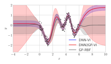
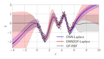
Figure 3: This figure shows a visualization of the predictive distributions on a modified version of the Snelson dataset [20]. The left figure shows Laplace and the right one shows VI. DNN2GP is our proposed method, elaborated upon in Appendix B, while DNN refers to a diagonal Gaussian approximation. We also compare to a GP with RBF kernel (GP-RBF). An MLP is used for DNN2GP and DNN. We see that, wherever the data is missing, the uncertainties are larger for our method than the others. For classification, we give an example in Fig. 9 in the appendix.

5.1 Comparison of DNN2GP Uncertainty

In this section, we visualize the quality of the uncertainty of the GP obtained with our DNN2GP approach on a simple regression task. To approximate predicitive uncertainty for our approach, we use the method described in Appendix B. We use both Laplace and VI approximations, referred to as ‘DNN2GP-Laplace’ and ‘DNN2GP-VI’, respectively. We compare it to the uncertainty obtained using an MC approximation in the DNN (referred to as ‘DNN-Laplace’ and ‘DNN-VI’). We also compare to a standard GP regression model with an RBF kernel (refer to as ‘GP-RBF’), whose kernel hyperparameters are chosen by optimizing the GP marginal likelihood.

We consider a version of the Snelson dataset [20] where, to assess the ‘in-between’ uncertainty, we remove the data points between x=1.5𝑥1.5x=1.5 and x=3𝑥3x=3. We use a single hidden-layer MLP with 32 units and sigmoidal transfer function. Fig. 3 shows the results for Laplace (left) and VI (right) approximation. For Laplace, we use Adam [11], and, for VI, we use VOGN [10]. The uncertainty provided by DNN2GP is bigger than the other methods wherever the data is not observed.

5.2 GP Kernel and Predictive Distribution for Classification Datasets

In this section, we visualize the GP kernel and predictive distribution for DNNs trained on CIFAR-10 and MNIST. Our goal is to show that our GP kernel and its predictions enhance our understanding of a DNN’s performance on classification tasks. We consider LeNet-5 [12] and compute both the Laplace and VI approximations. We show the visualization at the posterior mean.

The K×K𝐾𝐾K\times K GP kernel 𝜿(𝐱,𝐱):=𝐉(𝐱)𝐉(𝐱)assignsubscript𝜿𝐱superscript𝐱subscript𝐉𝐱subscript𝐉superscriptsuperscript𝐱top\mbox{$\mbox{$\boldsymbol{\kappa}$}$}_{*}(\mbox{$\mbox{$\mathbf{x}$}$},\mbox{$\mbox{$\mathbf{x}$}$}^{\prime}):=\mbox{$\mbox{$\mathbf{J}$}$}_{*}(\mbox{$\mbox{$\mathbf{x}$}$})\mbox{$\mbox{$\mathbf{J}$}$}_{*}(\mbox{$\mbox{$\mathbf{x}$}$}^{\prime})^{\top} results in a kernel matrix of dimensionality NK×NK𝑁𝐾𝑁𝐾NK\times NK which makes it difficult to visualize for our datasets. To simplify, we compute the sum of the diagonal entries of 𝜿(𝐱,𝐱)subscript𝜿𝐱superscript𝐱\mbox{$\mbox{$\boldsymbol{\kappa}$}$}_{*}(\mbox{$\mbox{$\mathbf{x}$}$},\mbox{$\mbox{$\mathbf{x}$}$}^{\prime}) to get an N×N𝑁𝑁N\times N matrix. This corresponds to modelling the output for each class with an individual GP and then summing the kernels of these GPs. We also visualize the GP posterior mean: 𝔼[𝐟(𝐱)|𝒟]=𝔼[𝐉(𝐱)𝐰|𝒟]=𝐉(𝐱)𝐰K\mathbb{E}[\mbox{$\mbox{$\mathbf{f}$}$}(\mbox{$\mbox{$\mathbf{x}$}$})|\mbox{${\cal D}$}]=\mathbb{E}[\mbox{$\mbox{$\mathbf{J}$}$}_{*}(\mbox{$\mbox{$\mathbf{x}$}$})\mbox{$\mbox{$\mathbf{w}$}$}|\mbox{${\cal D}$}]=\mbox{$\mbox{$\mathbf{J}$}$}_{*}(\mbox{$\mbox{$\mathbf{x}$}$})\mbox{$\mbox{$\mathbf{w}$}$}_{*}\in{}^{K}. and use the reparameterization that allows to predict in the data space 𝐲𝐲\mathbf{y} instead of 𝐲~~𝐲\tilde{\mbox{$\mbox{$\mathbf{y}$}$}} which is explained in Appendix B.
Refer to caption
Refer to caption
(a) MNIST: GP posterior mean (left) and GP kernel matrix (right)
Refer to caption
(b) CIFAR: GP posterior mean
Refer to caption
Refer to caption
(c) Binary-MNIST on digits 0 and 1
Refer to caption
Refer to caption
(d) Epistemic (left) and aleatoric (right) uncertainties
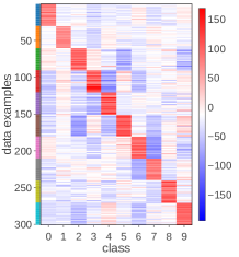
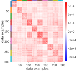
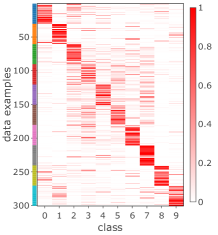
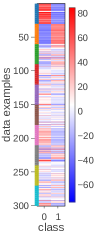
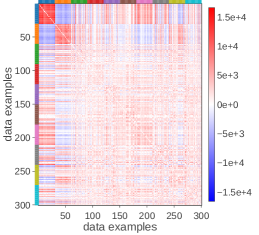
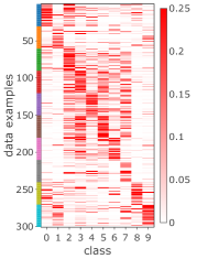
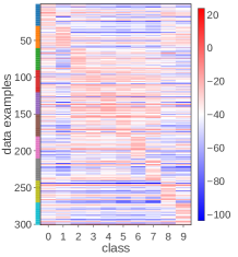
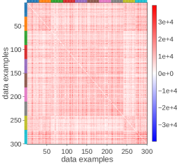
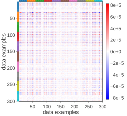
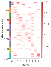
Figure 4: DNN2GP kernels, posterior means and uncertainties with LeNet5 of 300 samples on binary MNIST in Fig. (c), MNIST in Fig. (a), and CIFAR-10 in Fig. (b,d). The colored regions on the y-axis mark the classes. Fig. (a) shows the kernel and the predictive mean for the Laplace approximation, which gives 99% test accuracy. We see in the kernel that examples with same class labels are correlated. Fig. (c) shows the same for binary MNIST trained only on digits 0 and 1 by using VI. The kernel clearly shows the out-of-class predictive behavior where predictions are not certain. Fig. (b) and (d) show the Laplace-GP on the more complex CIFAR-10 data set where we obtain 68% accuracy. Fig. (d) shows the two components of the predictive variance for CIFAR-10 that can be interpreted as epistemic (left) and aleatoric (right) uncertainties. The estimated epistemic uncertainty is much lower than the aleatoric uncertainty, implying that the model is not flexible enough. This is plausible since the accuracy of the model is not too high (merely 68%).

Fig. 4 shows the GP kernel matrix and the posterior mean for the Laplace approximation on MNIST. The rows and columns containing 300 data examples are grouped according to the classes. The kernel matrix clearly shows the correlations learned by the DNN. As expected, each row in the posterior mean also reflects that the classes are correctly classified (DNN test accuracy is 99%). Fig. 4 shows the GP posterior mean after reparameterization for CIFAR-10 where we see a more noisy pattern due to a lower accuracy of around 68% on this task.

Fig. 4 shows the two components of the predictive variances that can be interpreted as “aleatoric” and “epistemic” uncertainty. As shown in Eq. (63) in Appendix B.2, for a multiclass classification loss, the variance of the prediction of a label at an input 𝐱subscript𝐱\mbox{$\mbox{$\mathbf{x}$}$}_{*} is equal to 𝚲(𝐱)+𝚲(𝐱)𝐉(𝐱)𝚺~𝐉(𝐱)𝚲(𝐱)subscript𝚲subscript𝐱subscript𝚲subscript𝐱subscript𝐉subscript𝐱~𝚺subscript𝐉superscriptsubscript𝐱topsubscript𝚲subscript𝐱\mbox{$\mbox{$\boldsymbol{\Lambda}$}$}_{*}(\mbox{$\mbox{$\mathbf{x}$}$}_{*})+\mbox{$\mbox{$\boldsymbol{\Lambda}$}$}_{*}(\mbox{$\mbox{$\mathbf{x}$}$}_{*})\mbox{$\mbox{$\mathbf{J}$}$}_{*}(\mbox{$\mbox{$\mathbf{x}$}$}_{*})\widetilde{\mbox{$\mbox{$\boldsymbol{\Sigma}$}$}}\mbox{$\mbox{$\mathbf{J}$}$}_{*}(\mbox{$\mbox{$\mathbf{x}$}$}_{*})^{\top}\mbox{$\mbox{$\boldsymbol{\Lambda}$}$}_{*}(\mbox{$\mbox{$\mathbf{x}$}$}_{*}). Similar to the linear basis function model, the two terms here have an interpretation (e.g., see Eq. 3.59 in [1]). The first term can be interpreted as the aleatoric uncertainty (label noise), while the second term takes a form that resembles the epistemic uncertainty (model noise). Fig. 4 shows these for CIFAR-10 where we see that the uncertainty of the model is low (left) and the label noise rather high (right). This interpretation implies that the model is unable to flexibly model the data and instead explains it with high label noise.

In Fig. 4, we study the kernel for classes outside of the training dataset using VI. We train LeNet-5 on digits 0 and 1 with VOGN and visualize the predictive mean and kernel on all 10 classes denoted by differently colored regions on the y-axis. We can see that there are slight correlations to the out-of-class samples but no overconfident predictions. In contrast, the pattern between 0 and 1 is quite strong. The kernel obtained with DNN2GP helps to interpret and visualize such correlations.

5.3 Tuning the Hyperparameters of a DNN Using the GP Marginal Likelihood

In this section, we demonstrate the tuning of DNN hyperparameters by using the GP marginal likelihood on a real and synthetic regression dataset. In the deep-learning literature, this is usually done using cross-validation. Our goal is to demonstrate that with DNN2GP we can do this by simply computing the marginal likelihood on the training set.
Refer to caption
(a) Model fits
Refer to caption
(b) Laplace Approximation
Refer to caption
(c) Variational Inference
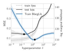
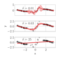
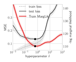
Figure 5: This figure demonstrates the use of the GP marginal likelihood to tune hyperparameters of a DNN. We tune the regularization parameter δ𝛿\delta on a synthetic dataset shown in (a). Fig. (b) and (c) show train and test MSE along with log of the marginal likelihoods on training data obtained with Laplace and VI respectively. We show the standard error over 10 runs. The optimal hyperparameters according to test loss and marginal-likelihood (shown with black stars) match well.
Refer to caption
Refer to caption
Refer to caption
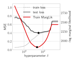
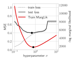
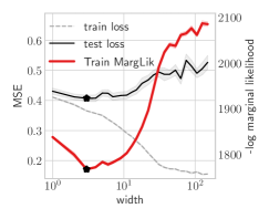
Figure 6: This is same as Fig. 5 but on a real dataset: UCI Red Wine Quality. All the plots use Laplace approximation, and the standard errors are estimated over 20 splits. We tune the following hyperparameters: the regularization parameter δ𝛿\delta (left), the noise-variance σ𝜎\sigma (middle), and the DNN width (right). The train log marginal-likelihood chooses hyperparameters that give a low test error.

We generate a synthetic regression dataset (N=100𝑁100N=100; see Fig. 5) where there are a few data points around x=0𝑥0x=0 but plenty away from it. We fit the data by using a neural network with single hidden layer of 20 units and tanh\tanh nonlinearity. Our goal is to tune the regularization parameter δ𝛿\delta to trade-off underfitting vs overfitting. Fig. 5 and 5 show the train log marginal-likelihood obtained with the GP obtained by DNN2GP, along with the test and train mean-square error (MSE) obtained using a point estimate. Black stars indicate the hyperparameters chosen by using the test loss and log marginal likelihood, respectively. We clearly see that the train marginal-likelihood chooses hyperparameters that give low test error. The train MSE on the other hand overfits as δ𝛿\delta is reduced.

Next, we discuss results for a real dataset: UCI Red Wine Quality (N=1599𝑁1599N=1599) with an input-dimensionality of 12 and a scalar output. We use an MLP with 2 hidden layers 20 units each and tanh\tanh transfer function. We consider tuning the regularizer δ𝛿\delta, the noise-variance σ𝜎\sigma, and the DNN width. We use the Laplace approximation and tune one parameter at a time while keeping the others fixed (we use respectively σ=0.64𝜎0.64\sigma=0.64, δ=30𝛿30\delta=30 and σ=0.64𝜎0.64\sigma=0.64, δ=3𝛿3\delta=3, 111 hidden layer). Similarly to the synthetic data case, the train marginal-likelihood selects hyperparameters that give low test error. These experiments show that the DNN2GP framework can be useful to tune DNN hyperparameters, although this needs to be confirmed for larger networks than we used here.

6 Discussion and Future Work

In this paper, we present theoretical results connecting approximate inference on DNNs to GP posteriors. Our work enables the extraction of feature maps and GP kernels by simply training DNNs. It provides a natural way to combine the two different models.

Our hope is that our theoretical results will facilitate further research on combining strengths of DNNs and GPs. A computational bottleneck is the Jacobian computation which prohibits application to large problems. There are several ways to reduce this computation, e.g., by choosing a different type of GGN approximation that uses gradients instead of the Jacobians. Exploration of such methods is a future direction that needs to be pursued.

Exact inference on the GP model we derive is still computationally infeasible for large problems. However, further approximations could enable inference on bigger datasets. Finally, our work opens many other interesting avenues where a combination of GPs and DNNs can be useful such as model selection, deep reinforcement learning, Bayesian optimization, active learning, interpretation, etc. We hope that our work enables the community to conduct further research on such problems.
Acknowledgements

We would like to thank Kazuki Osawa (Tokyo Institute of Technology), Anirudh Jain (RIKEN), and Runa Eschenhagen (RIKEN) for their help with the experiments. We would also like to thank Matthias Bauer (DeepMind) for discussions and useful feedback. Many thanks to Roman Bachmann (RIKEN) for helping with the visualization in Fig. 1. We also thank Stephan Mandt (UCI) for suggesting the marginal likelihood experiment. We thank the reviewers and the area chair for their feedback as well. We are also thankful for the RAIDEN computing system and its support team at the RIKEN Center for Advanced Intelligence Project which we used extensively for our experiments.

References

  • Bishop [2006] Christopher M Bishop. Pattern recognition and machine learning. springer, 2006.
  • Bottou et al. [2018] L. Bottou, F. Curtis, and J. Nocedal. Optimization methods for large-scale machine learning. SIAM Review, 60(2):223–311, 2018. doi: 10.1137/16M1080173.
  • Bradshaw et al. [2017] John Bradshaw, Alexander G de G Matthews, and Zoubin Ghahramani. Adversarial examples, uncertainty, and transfer testing robustness in Gaussian process hybrid deep networks. arXiv preprint arXiv:1707.02476, 2017.
  • Cho and Saul [2009] Youngmin Cho and Lawrence K. Saul. Kernel methods for deep learning. In Y. Bengio, D. Schuurmans, J. D. Lafferty, C. K. I. Williams, and A. Culotta, editors, Advances in Neural Information Processing Systems 22, pages 342–350. Curran Associates, Inc., 2009.
  • de G. Matthews et al. [2018] Alexander G. de G. Matthews, Jiri Hron, Mark Rowland, Richard E. Turner, and Zoubin Ghahramani. Gaussian process behaviour in wide deep neural networks. In International Conference on Learning Representations, 2018.
  • Garriga-Alonso et al. [2019] Adrià Garriga-Alonso, Carl Edward Rasmussen, and Laurence Aitchison. Deep convolutional networks as shallow Gaussian processes. In International Conference on Learning Representations, 2019.
  • Hazan and Jaakkola [2015] Tamir Hazan and Tommi S. Jaakkola. Steps toward deep kernel methods from infinite neural networks. CoRR, abs/1508.05133, 2015.
  • Jacot et al. [2018] Arthur Jacot, Franck Gabriel, and Clement Hongler. Neural tangent kernel: Convergence and generalization in neural networks. In S. Bengio, H. Wallach, H. Larochelle, K. Grauman, N. Cesa-Bianchi, and R. Garnett, editors, Advances in Neural Information Processing Systems 31, pages 8571–8580. Curran Associates, Inc., 2018.
  • Khan [2012] Mohammad Khan. Variational learning for latent Gaussian model of discrete data. PhD thesis, University of British Columbia, 2012.
  • Khan et al. [2018] Mohammad Emtiyaz Khan, Didrik Nielsen, Voot Tangkaratt, Wu Lin, Yarin Gal, and Akash Srivastava. Fast and scalable Bayesian deep learning by weight-perturbation in Adam. In International Conference on Machine Learning, pages 2616–2625, 2018.
  • Kingma and Ba [2014] Diederik P Kingma and Jimmy Ba. Adam: A method for stochastic optimization. arXiv preprint arXiv:1412.6980, 2014.
  • LeCun et al. [1998] Yann LeCun, Léon Bottou, Yoshua Bengio, Patrick Haffner, et al. Gradient-based learning applied to document recognition. Proceedings of the IEEE, 86(11):2278–2324, 1998.
  • Lee et al. [2018] Jaehoon Lee, Yasaman Bahri, Roman Novak, Samuel S. Schoenholz, Jeffrey Pennington, and Jascha Sohl-Dickstein. Deep neural networks as Gaussian processes. In 6th International Conference on Learning Representations, ICLR 2018, Vancouver, BC, Canada, April 30 - May 3, 2018, Conference Track Proceedings, 2018.
  • Lee et al. [2019] Jaehoon Lee, Lechao Xiao, Samuel S. Schoenholz, Yasaman Bahri, Roman Novak, Jascha Sohl-Dickstein, and Jeffrey Pennington. Wide Neural Networks of Any Depth Evolve as Linear Models Under Gradient Descent. arXiv e-prints, art. arXiv:1902.06720, Feb 2019.
  • Martens [2014] James Martens. New perspectives on the natural gradient method. CoRR, abs/1412.1193, 2014.
  • Neal [1996] Radford M. Neal. Bayesian Learning for Neural Networks. Springer-Verlag, Berlin, Heidelberg, 1996. ISBN 0387947248.
  • Nocedal and Wright [2006] Jorge Nocedal and Stephen Wright. Numerical optimization. Springer Science & Business Media, 2006.
  • Novak et al. [2019] Roman Novak, Lechao Xiao, Yasaman Bahri, Jaehoon Lee, Greg Yang, Daniel A. Abolafia, Jeffrey Pennington, and Jascha Sohl-dickstein. Bayesian deep convolutional networks with many channels are Gaussian processes. In International Conference on Learning Representations, 2019.
  • Osawa et al. [2019] Kazuki Osawa, Siddharth Swaroop, Anirudh Jain, Runa Eschenhagen, Richard Turner, Rio Yokota, and Mohammad Emtiyaz Khan. Practical deep learning with Bayesian principles. In Advances in Neural Information Processing Systems, 2019.
  • Snelson and Ghahramani [2006] Edward Snelson and Zoubin Ghahramani. Sparse gaussian processes using pseudo-inputs. In Y. Weiss, B. Schölkopf, and J. C. Platt, editors, Advances in Neural Information Processing Systems 18, pages 1257–1264. MIT Press, 2006.
  • Tieleman and Hinton [2012] Tijmen Tieleman and Geoffrey Hinton. Lecture 6.5-RMSprop: Divide the gradient by a running average of its recent magnitude. COURSERA: Neural Networks for Machine Learning 4, 2012.
  • Williams [1997] Christopher KI Williams. Computing with infinite networks. In Advances in neural information processing systems, pages 295–301, 1997.
  • Williams and Rasmussen [2006] Christopher KI Williams and Carl Edward Rasmussen. Gaussian processes for machine learning, volume 2. MIT Press Cambridge, MA, 2006.

Appendix A Proofs

In this section, we prove the theorems presented in the main text.

A.1 Proof of Theorem 1

We begin with the Gaussian approximation of the Laplace approximation. We will then express its natural parameters in terms of the gradient and Hessians. Application of the GGN approximation and some further manipulation will show that the distribution correspond to the posterior of a linear model.

We start with the Laplace approximation (4) and express its natural parameters in terms of the gradient and Hessians. We denote the natural-parameters of this Gaussian approximation 𝒩(𝐰|𝝁,𝚺)𝒩conditional𝐰𝝁𝚺\mbox{${\cal N}$}(\mbox{$\mbox{$\mathbf{w}$}$}|\mbox{$\mbox{$\boldsymbol{\mu}$}$},\mbox{$\mbox{$\boldsymbol{\Sigma}$}$}) by 𝜼:={𝚺1𝝁,12𝚺1}assign𝜼superscript𝚺1𝝁superscript12𝚺1\mbox{$\mbox{$\boldsymbol{\eta}$}$}:=\{\mbox{$\mbox{$\boldsymbol{\Sigma}$}$}^{-1}\mbox{$\mbox{$\boldsymbol{\mu}$}$},-\mbox{$\frac{1}{2}$}\mbox{$\mbox{$\boldsymbol{\Sigma}$}$}^{-1}\}. In (4), the second natural parameter is set to the following which is written in terms of the Hessian:

12𝚺1=12[i=1Nww2i(𝐰)+δ𝐈P].superscript12𝚺112delimited-[]superscriptsubscript𝑖1𝑁superscriptsubscript𝑤𝑤2subscript𝑖subscript𝐰𝛿subscript𝐈𝑃\displaystyle-\mbox{$\frac{1}{2}$}\mbox{$\mbox{$\boldsymbol{\Sigma}$}$}^{-1}=-\mbox{$\frac{1}{2}$}\left[\sum_{i=1}^{N}\nabla_{ww}^{2}\ell_{i}(\mbox{$\mbox{$\mathbf{w}$}$}_{*})+\delta\mbox{$\mbox{$\mathbf{I}$}$}_{P}\right]. (15)

We can also express the first natural parameter in terms of the gradient and Hessians as shown below. We use the first-order stationary condition, that is, w¯(𝒟,𝐰)=0subscript𝑤¯𝒟subscript𝐰0\nabla_{w}\bar{\ell}(\mbox{${\cal D}$},\mbox{$\mbox{$\mathbf{w}$}$}_{*})=0. Adding 𝚺1𝝁superscript𝚺1𝝁\mbox{$\mbox{$\boldsymbol{\Sigma}$}$}^{-1}\mbox{$\mbox{$\boldsymbol{\mu}$}$} to the both sides of this condition, we get the following:

𝚺1𝝁superscript𝚺1𝝁\displaystyle\mbox{$\mbox{$\boldsymbol{\Sigma}$}$}^{-1}\mbox{$\mbox{$\boldsymbol{\mu}$}$} =w¯(𝒟,𝐰)+𝚺1𝝁absentsubscript𝑤¯𝒟subscript𝐰superscript𝚺1𝝁\displaystyle=-\nabla_{w}\bar{\ell}(\mbox{${\cal D}$},\mbox{$\mbox{$\mathbf{w}$}$}_{*})+\mbox{$\mbox{$\boldsymbol{\Sigma}$}$}^{-1}\mbox{$\mbox{$\boldsymbol{\mu}$}$} (16)
=i=1Nwi(𝐰)δ𝐰+[i=1Nww2i(𝐰)+δ𝐈P]𝐰absentsuperscriptsubscript𝑖1𝑁subscript𝑤subscript𝑖subscript𝐰𝛿subscript𝐰delimited-[]superscriptsubscript𝑖1𝑁superscriptsubscript𝑤𝑤2subscript𝑖subscript𝐰𝛿subscript𝐈𝑃subscript𝐰\displaystyle=-\sum_{i=1}^{N}\nabla_{w}\ell_{i}(\mbox{$\mbox{$\mathbf{w}$}$}_{*})-\delta\mbox{$\mbox{$\mathbf{w}$}$}_{*}+\left[\sum_{i=1}^{N}\nabla_{ww}^{2}\ell_{i}(\mbox{$\mbox{$\mathbf{w}$}$}_{*})+\delta\mbox{$\mbox{$\mathbf{I}$}$}_{P}\right]\mbox{$\mbox{$\mathbf{w}$}$}_{*} (17)
=i=1N[wi(𝐰)+ww2i(𝐰)𝐰],absentsuperscriptsubscript𝑖1𝑁delimited-[]subscript𝑤subscript𝑖subscript𝐰superscriptsubscript𝑤𝑤2subscript𝑖subscript𝐰subscript𝐰\displaystyle=\sum_{i=1}^{N}\left[-\nabla_{w}\ell_{i}(\mbox{$\mbox{$\mathbf{w}$}$}_{*})+\nabla_{ww}^{2}\ell_{i}(\mbox{$\mbox{$\mathbf{w}$}$}_{*})\mbox{$\mbox{$\mathbf{w}$}$}_{*}\right], (18)

where in the second step, we substitute 𝝁𝝁\boldsymbol{\mu} by 𝐰subscript𝐰\mbox{$\mbox{$\mathbf{w}$}$}_{*} and also use (15). With this, both natural parameters are now expressed in terms of the gradient and Hessian.

We will now substitute these in the Laplace approximation, denoted by qL(𝐰):=𝒩(𝐰|𝝁,𝚺)assignsubscript𝑞𝐿𝐰𝒩conditional𝐰𝝁𝚺q_{L}(\mbox{$\mbox{$\mathbf{w}$}$}):=\mbox{${\cal N}$}(\mbox{$\mbox{$\mathbf{w}$}$}|\mbox{$\mbox{$\boldsymbol{\mu}$}$},\mbox{$\mbox{$\boldsymbol{\Sigma}$}$}). Using (15) and (18), we get the following expression:

qLsubscript𝑞𝐿\displaystyle q_{L} (𝐰)=1(2π)P|𝚺|exp[12(𝐰𝝁)𝚺1(𝐰𝝁)]𝐰1superscript2𝜋𝑃𝚺12superscript𝐰𝝁topsuperscript𝚺1𝐰𝝁\displaystyle(\mbox{$\mbox{$\mathbf{w}$}$})=\frac{1}{\sqrt{(2\pi)^{P}|\mbox{$\mbox{$\boldsymbol{\Sigma}$}$}|}}\exp{\left[-\mbox{$\frac{1}{2}$}(\mbox{$\mbox{$\mathbf{w}$}$}-\mbox{$\mbox{$\boldsymbol{\mu}$}$})^{\top}\mbox{$\mbox{$\boldsymbol{\Sigma}$}$}^{-1}(\mbox{$\mbox{$\mathbf{w}$}$}-\mbox{$\mbox{$\boldsymbol{\mu}$}$})\right]} (19)
exp[12𝐰(𝚺1)𝐰+𝐰(𝚺1𝝁)]proportional-toabsentsuperscript12𝐰topsuperscript𝚺1𝐰superscript𝐰topsuperscript𝚺1𝝁\displaystyle\propto\exp{\left[-\mbox{$\frac{1}{2}$}\mbox{$\mbox{$\mathbf{w}$}$}^{\top}(\mbox{$\mbox{$\boldsymbol{\Sigma}$}$}^{-1})\mbox{$\mbox{$\mathbf{w}$}$}+\mbox{$\mbox{$\mathbf{w}$}$}^{\top}(\mbox{$\mbox{$\boldsymbol{\Sigma}$}$}^{-1}\mbox{$\mbox{$\boldsymbol{\mu}$}$})\right]} (20)
=exp(δ𝐰𝐰2)i=1Nexp[12𝐰ww2i(𝐰)𝐰+𝐰{wi(𝐰)+ww2i(𝐰)𝐰}],absent𝛿superscript𝐰top𝐰2superscriptsubscriptproduct𝑖1𝑁superscript12𝐰topsuperscriptsubscript𝑤𝑤2subscript𝑖subscript𝐰𝐰superscript𝐰topsubscript𝑤subscript𝑖subscript𝐰superscriptsubscript𝑤𝑤2subscript𝑖subscript𝐰subscript𝐰\displaystyle=\exp{\left(\frac{-\delta\mbox{$\mbox{$\mathbf{w}$}$}^{\top}\mbox{$\mbox{$\mathbf{w}$}$}}{2}\right)}\prod_{i=1}^{N}\exp{\left[-\mbox{$\frac{1}{2}$}\mbox{$\mbox{$\mathbf{w}$}$}^{\top}\nabla_{ww}^{2}\ell_{i}(\mbox{$\mbox{$\mathbf{w}$}$}_{*})\mbox{$\mbox{$\mathbf{w}$}$}+\mbox{$\mbox{$\mathbf{w}$}$}^{\top}\left\{-\nabla_{w}\ell_{i}(\mbox{$\mbox{$\mathbf{w}$}$}_{*})+\nabla_{ww}^{2}\ell_{i}(\mbox{$\mbox{$\mathbf{w}$}$}_{*})\mbox{$\mbox{$\mathbf{w}$}$}_{*}\right\}\right]}, (21)

where in the last line we use (15) and (18).

Now, we will employ the GGN approximation (7) which gives us the Laplace-GGN approximation 𝒩(𝐰|𝝁,𝚺~)𝒩conditional𝐰𝝁~𝚺\mbox{${\cal N}$}(\mbox{$\mbox{$\mathbf{w}$}$}|\mbox{$\mbox{$\boldsymbol{\mu}$}$},\widetilde{\mbox{$\mbox{$\boldsymbol{\Sigma}$}$}}), shown below:

exp(δ𝐰𝐰2)i=1Nexp[12𝐰𝐉(𝐱i)𝚲i,𝐉(𝐱i)𝐰+𝐰𝐉(𝐱i){𝚲i,𝐉(𝐱i)𝐰𝐫i,}],𝛿superscript𝐰top𝐰2superscriptsubscriptproduct𝑖1𝑁12superscript𝐰topsubscript𝐉superscriptsubscript𝐱𝑖topsubscript𝚲𝑖subscript𝐉subscript𝐱𝑖𝐰superscript𝐰topsubscript𝐉superscriptsubscript𝐱𝑖topsubscript𝚲𝑖subscript𝐉subscript𝐱𝑖subscript𝐰subscript𝐫𝑖\exp{\left(\frac{-\delta\mbox{$\mbox{$\mathbf{w}$}$}^{\top}\mbox{$\mbox{$\mathbf{w}$}$}}{2}\right)}\prod_{i=1}^{N}\exp{\left[\frac{-1}{2}\mbox{$\mbox{$\mathbf{w}$}$}^{\top}\mbox{$\mbox{$\mathbf{J}$}$}_{*}(\mbox{$\mbox{$\mathbf{x}$}$}_{i})^{\top}\mbox{$\mbox{$\boldsymbol{\Lambda}$}$}_{i,*}\mbox{$\mbox{$\mathbf{J}$}$}_{*}(\mbox{$\mbox{$\mathbf{x}$}$}_{i})\mbox{$\mbox{$\mathbf{w}$}$}+\mbox{$\mbox{$\mathbf{w}$}$}^{\top}\mbox{$\mbox{$\mathbf{J}$}$}_{*}(\mbox{$\mbox{$\mathbf{x}$}$}_{i})^{\top}\left\{\mbox{$\mbox{$\boldsymbol{\Lambda}$}$}_{i,*}\mbox{$\mbox{$\mathbf{J}$}$}_{*}(\mbox{$\mbox{$\mathbf{x}$}$}_{i})\mbox{$\mbox{$\mathbf{w}$}$}_{*}-\mbox{$\mbox{$\mathbf{r}$}$}_{i,*}\right\}\right]}, (22)

where for notational convenience we have denoted 𝚲i,:=𝚲(𝐱i,𝐲i)assignsubscript𝚲𝑖subscript𝚲subscript𝐱𝑖subscript𝐲𝑖\mbox{$\mbox{$\boldsymbol{\Lambda}$}$}_{i,*}:=\mbox{$\mbox{$\boldsymbol{\Lambda}$}$}_{*}(\mbox{$\mbox{$\mathbf{x}$}$}_{i},\mbox{$\mbox{$\mathbf{y}$}$}_{i}) and 𝐫i,:=𝐫(𝐱i,𝐲i)assignsubscript𝐫𝑖subscript𝐫subscript𝐱𝑖subscript𝐲𝑖\mbox{$\mbox{$\mathbf{r}$}$}_{i,*}:=\mbox{$\mbox{$\mathbf{r}$}$}_{*}(\mbox{$\mbox{$\mathbf{x}$}$}_{i},\mbox{$\mbox{$\mathbf{y}$}$}_{i}).

A key point here is that each term in the product over i𝑖i in (22) is proportional to a Gaussian distribution, provided that 𝚲i,0succeedssubscript𝚲𝑖0\mbox{$\mbox{$\boldsymbol{\Lambda}$}$}_{i,*}\succ 0, which is the case since we assume the loss function to be strictly convex. We will now express each term in the product, as a likelihood over a pseudo-output defined as 𝐲~i:=𝐉(𝐱i)𝐰𝚲i,1𝐫i,assignsubscript~𝐲𝑖subscript𝐉subscript𝐱𝑖subscript𝐰superscriptsubscript𝚲𝑖1subscript𝐫𝑖\tilde{\mbox{$\mbox{$\mathbf{y}$}$}}_{i}:=\mbox{$\mbox{$\mathbf{J}$}$}_{*}(\mbox{$\mbox{$\mathbf{x}$}$}_{i})\mbox{$\mbox{$\mathbf{w}$}$}_{*}-\mbox{$\mbox{$\boldsymbol{\Lambda}$}$}_{i,*}^{-1}\mbox{$\mbox{$\mathbf{r}$}$}_{i,*}. Using this and completing the square within each term in the product over i𝑖i in (22), we get the following:

q~L(𝐰):=𝒩(𝐰|𝝁,𝚺~)𝒩(𝐰|0,δ1𝐈P)i=1N𝒩(𝐲~i|𝐉(𝐱i)𝐰,𝚲i,1).assignsubscript~𝑞𝐿𝐰𝒩conditional𝐰𝝁~𝚺proportional-to𝒩conditional𝐰0superscript𝛿1subscript𝐈𝑃superscriptsubscriptproduct𝑖1𝑁𝒩conditionalsubscript~𝐲𝑖subscript𝐉subscript𝐱𝑖𝐰superscriptsubscript𝚲𝑖1\tilde{q}_{L}(\mbox{$\mbox{$\mathbf{w}$}$}):=\mbox{${\cal N}$}(\mbox{$\mbox{$\mathbf{w}$}$}|\mbox{$\mbox{$\boldsymbol{\mu}$}$},\widetilde{\mbox{$\mbox{$\boldsymbol{\Sigma}$}$}})\propto\mbox{${\cal N}$}(\mbox{$\mbox{$\mathbf{w}$}$}|0,\delta^{-1}\mbox{$\mbox{$\mathbf{I}$}$}_{P})\prod_{i=1}^{N}\mbox{${\cal N}$}(\tilde{\mbox{$\mbox{$\mathbf{y}$}$}}_{i}|\mbox{$\mbox{$\mathbf{J}$}$}_{*}(\mbox{$\mbox{$\mathbf{x}$}$}_{i})\mbox{$\mbox{$\mathbf{w}$}$},\mbox{$\mbox{$\boldsymbol{\Lambda}$}$}_{i,*}^{-1}). (23)

The right hand side of the above equation is proportional to the posterior distribution p(𝐰|𝒟~)𝑝conditional𝐰~𝒟p(\mbox{$\mbox{$\mathbf{w}$}$}|\widetilde{\mbox{${\cal D}$}}) given a transformed dataset 𝒟~:={(𝐱i,𝐲~i)}i=1Nassign~𝒟superscriptsubscriptsubscript𝐱𝑖subscript~𝐲𝑖𝑖1𝑁\widetilde{\mbox{${\cal D}$}}:=\{(\mbox{$\mbox{$\mathbf{x}$}$}_{i},\tilde{\mbox{$\mbox{$\mathbf{y}$}$}}_{i})\}_{i=1}^{N} of a linear basis-function model 𝐲~=𝐉(𝐱)𝐰+ϵ~𝐲subscript𝐉𝐱𝐰bold-italic-ϵ\tilde{\mbox{$\mbox{$\mathbf{y}$}$}}=\mbox{$\mbox{$\mathbf{J}$}$}_{*}(\mbox{$\mbox{$\mathbf{x}$}$})\mbox{$\mbox{$\mathbf{w}$}$}+\mbox{$\mbox{$\boldsymbol{\epsilon}$}$} with Gaussian noise ϵ𝒩(0,(𝚲(𝐱,𝐲))1)similar-tobold-italic-ϵ𝒩0superscriptsubscript𝚲𝐱𝐲1\mbox{$\mbox{$\boldsymbol{\epsilon}$}$}\sim\mbox{${\cal N}$}(0,(\mbox{$\mbox{$\boldsymbol{\Lambda}$}$}_{*}(\mbox{$\mbox{$\mathbf{x}$}$},\mbox{$\mbox{$\mathbf{y}$}$}))^{-1}) and prior distribution 𝐰𝒩(0,δ1𝐈P)similar-to𝐰𝒩0superscript𝛿1subscript𝐈𝑃\mbox{$\mbox{$\mathbf{w}$}$}\sim\mbox{${\cal N}$}(0,\delta^{-1}\mbox{$\mbox{$\mathbf{I}$}$}_{P}). This completes the proof.

It is easy to see that the same proof works when using the approximations shown in (5). In that case, only the steps from (22) need to be modified. The proof also holds when a prior other than Gaussian and a model other than DNN is used. ∎

A.2 Proof of Theorem 2

Similarly to the previous section, we start by writing the Gaussian approximation for VON. We will express its natural parameters in terms of the gradient and Hessians. A GGN approximation and some manipulation will show that the distributions found by VON correspond to posteriors of linear models.

The Gaussian approximation at the t𝑡t’th iteration of VON is denoted by qt(𝐰):=𝒩(𝐰|𝝁t,𝚺t)assignsubscript𝑞𝑡𝐰𝒩conditional𝐰subscript𝝁𝑡subscript𝚺𝑡q_{t}(\mbox{$\mbox{$\mathbf{w}$}$}):=\mbox{${\cal N}$}(\mbox{$\mbox{$\mathbf{w}$}$}|\mbox{$\mbox{$\boldsymbol{\mu}$}$}_{t},\mbox{$\mbox{$\boldsymbol{\Sigma}$}$}_{t}) where 𝚺t:=(𝐒t+δ𝐈P)1assignsubscript𝚺𝑡superscriptsubscript𝐒𝑡𝛿subscript𝐈𝑃1\mbox{$\mbox{$\boldsymbol{\Sigma}$}$}_{t}:=(\mbox{$\mbox{$\mathbf{S}$}$}_{t}+\delta\mbox{$\mbox{$\mathbf{I}$}$}_{P})^{-1} is obtained from 𝐒tsubscript𝐒𝑡\mbox{$\mbox{$\mathbf{S}$}$}_{t}. Using this, we can rewrite the updates (11) and (12) in terms of 𝝁tsubscript𝝁𝑡\mbox{$\mbox{$\boldsymbol{\mu}$}$}_{t} and 𝚺t1superscriptsubscript𝚺𝑡1\mbox{$\mbox{$\boldsymbol{\Sigma}$}$}_{t}^{-1} as follows

𝝁t+1subscript𝝁𝑡1\displaystyle\mbox{$\mbox{$\boldsymbol{\mu}$}$}_{t+1} =𝝁tβt𝚺t+1[i=1N𝔼qt(w)[wi(𝐰)]+δ𝝁t],absentsubscript𝝁𝑡subscript𝛽𝑡subscript𝚺𝑡1delimited-[]superscriptsubscript𝑖1𝑁subscript𝔼subscript𝑞𝑡𝑤delimited-[]subscript𝑤subscript𝑖𝐰𝛿subscript𝝁𝑡\displaystyle=\mbox{$\mbox{$\boldsymbol{\mu}$}$}_{t}-\beta_{t}\mbox{$\mbox{$\boldsymbol{\Sigma}$}$}_{t+1}\left[\sum_{i=1}^{N}\mathbb{E}_{q_{t}(w)}\left[\nabla_{w}\ell_{i}(\mbox{$\mbox{$\mathbf{w}$}$})\right]+\delta\mbox{$\mbox{$\boldsymbol{\mu}$}$}_{t}\right], (24)
𝚺t+11superscriptsubscript𝚺𝑡11\displaystyle\mbox{$\mbox{$\boldsymbol{\Sigma}$}$}_{t+1}^{-1} =(1βt)𝚺t1+βt[i=1N𝔼qt(w)[ww2i(𝐰)]+δ𝐈P].absent1subscript𝛽𝑡superscriptsubscript𝚺𝑡1subscript𝛽𝑡delimited-[]superscriptsubscript𝑖1𝑁subscript𝔼subscript𝑞𝑡𝑤delimited-[]superscriptsubscript𝑤𝑤2subscript𝑖𝐰𝛿subscript𝐈𝑃\displaystyle=(1-\beta_{t})\mbox{$\mbox{$\boldsymbol{\Sigma}$}$}_{t}^{-1}+\beta_{t}\left[\sum_{i=1}^{N}\mathbb{E}_{q_{t}(w)}\left[\nabla_{ww}^{2}\ell_{i}(\mbox{$\mbox{$\mathbf{w}$}$})\right]+\delta\mbox{$\mbox{$\mathbf{I}$}$}_{P}\right]. (25)

It is again more convenient if we can have an update formula for the natural-parameters of the Gaussian distribution 𝒩(𝐰|𝝁t,𝚺t)𝒩conditional𝐰subscript𝝁𝑡subscript𝚺𝑡\mbox{${\cal N}$}(\mbox{$\mbox{$\mathbf{w}$}$}|\mbox{$\mbox{$\boldsymbol{\mu}$}$}_{t},\mbox{$\mbox{$\boldsymbol{\Sigma}$}$}_{t}), denoted by 𝜼t:={𝚺t1𝝁t,12𝚺t1}assignsubscript𝜼𝑡superscriptsubscript𝚺𝑡1subscript𝝁𝑡superscriptsubscript12𝚺𝑡1\mbox{$\mbox{$\boldsymbol{\eta}$}$}_{t}:=\{\mbox{$\mbox{$\boldsymbol{\Sigma}$}$}_{t}^{-1}\mbox{$\mbox{$\boldsymbol{\mu}$}$}_{t},-\mbox{$\frac{1}{2}$}\mbox{$\mbox{$\boldsymbol{\Sigma}$}$}_{t}^{-1}\}. So we use similar techniques to find an update for 𝜼tsubscript𝜼𝑡\mbox{$\mbox{$\boldsymbol{\eta}$}$}_{t}. In addition, since there are no closed-form expressions for the expectations above, we use S𝑆S number of samples 𝐰t(s)qt(𝐰)similar-tosuperscriptsubscript𝐰𝑡𝑠subscript𝑞𝑡𝐰\mbox{$\mbox{$\mathbf{w}$}$}_{t}^{(s)}\sim q_{t}(\mbox{$\mbox{$\mathbf{w}$}$}), for s=1,2,,S𝑠12𝑆s=1,2,\ldots,S, and use Monte Carlo (MC) approximation.

Given (25), the update corresponding to the second natural-parameter is obvious and given by

12𝚺t+11superscriptsubscript12𝚺𝑡11\displaystyle-\mbox{$\frac{1}{2}$}\mbox{$\mbox{$\boldsymbol{\Sigma}$}$}_{t+1}^{-1} =(1βt)[12𝚺t1]12βt[i=1N𝔼qt(w)[ww2i(𝐰)]+δ𝐈P]absent1subscript𝛽𝑡delimited-[]superscriptsubscript12𝚺𝑡112subscript𝛽𝑡delimited-[]superscriptsubscript𝑖1𝑁subscript𝔼subscript𝑞𝑡𝑤delimited-[]superscriptsubscript𝑤𝑤2subscript𝑖𝐰𝛿subscript𝐈𝑃\displaystyle=(1-\beta_{t})\left[-\mbox{$\frac{1}{2}$}\mbox{$\mbox{$\boldsymbol{\Sigma}$}$}_{t}^{-1}\right]-\mbox{$\frac{1}{2}$}\beta_{t}\left[\sum_{i=1}^{N}\mathbb{E}_{q_{t}(w)}\left[\nabla_{ww}^{2}\ell_{i}(\mbox{$\mbox{$\mathbf{w}$}$})\right]+\delta\mbox{$\mbox{$\mathbf{I}$}$}_{P}\right] (26)
(1βt)[12𝚺t1]12βt[1Si,s=1N,Sww2i(𝐰t(s))+δ𝐈P],absent1subscript𝛽𝑡delimited-[]superscriptsubscript12𝚺𝑡112subscript𝛽𝑡delimited-[]1𝑆superscriptsubscript𝑖𝑠1𝑁𝑆superscriptsubscript𝑤𝑤2subscript𝑖superscriptsubscript𝐰𝑡𝑠𝛿subscript𝐈𝑃\displaystyle\approx(1-\beta_{t})\left[-\mbox{$\frac{1}{2}$}\mbox{$\mbox{$\boldsymbol{\Sigma}$}$}_{t}^{-1}\right]-\mbox{$\frac{1}{2}$}\beta_{t}\left[\frac{1}{S}\sum_{i,s=1}^{N,S}\nabla_{ww}^{2}\ell_{i}(\mbox{$\mbox{$\mathbf{w}$}$}_{t}^{(s)})+\delta\mbox{$\mbox{$\mathbf{I}$}$}_{P}\right], (27)

where we have used an MC approximation in the second step.

To write the update for the first natural-parameter, we multiply (24) by 𝚺t+11superscriptsubscript𝚺𝑡11\mbox{$\mbox{$\boldsymbol{\Sigma}$}$}_{t+1}^{-1} and get

𝚺t+11𝝁t+1superscriptsubscript𝚺𝑡11subscript𝝁𝑡1\displaystyle\mbox{$\mbox{$\boldsymbol{\Sigma}$}$}_{t+1}^{-1}\mbox{$\mbox{$\boldsymbol{\mu}$}$}_{t+1} =𝚺t+11𝝁tβt[i=1N𝔼qt(w)[wi(𝐰)]+δ𝝁t]absentsuperscriptsubscript𝚺𝑡11subscript𝝁𝑡subscript𝛽𝑡delimited-[]superscriptsubscript𝑖1𝑁subscript𝔼subscript𝑞𝑡𝑤delimited-[]subscript𝑤subscript𝑖𝐰𝛿subscript𝝁𝑡\displaystyle=\mbox{$\mbox{$\boldsymbol{\Sigma}$}$}_{t+1}^{-1}\mbox{$\mbox{$\boldsymbol{\mu}$}$}_{t}-\beta_{t}\left[\sum_{i=1}^{N}\mathbb{E}_{q_{t}(w)}\left[\nabla_{w}\ell_{i}(\mbox{$\mbox{$\mathbf{w}$}$})\right]+\delta\mbox{$\mbox{$\boldsymbol{\mu}$}$}_{t}\right] (28)
=(1βt)[𝚺t1𝝁t]+βti=1N[𝔼qt(w)[wi(𝐰)]+𝔼qt(w)[ww2i(𝐰)]𝝁t]absent1subscript𝛽𝑡delimited-[]superscriptsubscript𝚺𝑡1subscript𝝁𝑡subscript𝛽𝑡superscriptsubscript𝑖1𝑁delimited-[]subscript𝔼subscript𝑞𝑡𝑤delimited-[]subscript𝑤subscript𝑖𝐰subscript𝔼subscript𝑞𝑡𝑤delimited-[]superscriptsubscript𝑤𝑤2subscript𝑖𝐰subscript𝝁𝑡\displaystyle=(1-\beta_{t})\left[\mbox{$\mbox{$\boldsymbol{\Sigma}$}$}_{t}^{-1}\mbox{$\mbox{$\boldsymbol{\mu}$}$}_{t}\right]+\beta_{t}\sum_{i=1}^{N}\left[-\mathbb{E}_{q_{t}(w)}\left[\nabla_{w}\ell_{i}(\mbox{$\mbox{$\mathbf{w}$}$})\right]+\mathbb{E}_{q_{t}(w)}\left[\nabla_{ww}^{2}\ell_{i}(\mbox{$\mbox{$\mathbf{w}$}$})\right]\mbox{$\mbox{$\boldsymbol{\mu}$}$}_{t}\right] (29)
(1βt)[𝚺t1𝝁t]+βtSi,s=1N,S[wi(𝐰t(s))+ww2i(𝐰t(s))𝝁t],absent1subscript𝛽𝑡delimited-[]superscriptsubscript𝚺𝑡1subscript𝝁𝑡subscript𝛽𝑡𝑆superscriptsubscript𝑖𝑠1𝑁𝑆delimited-[]subscript𝑤subscript𝑖superscriptsubscript𝐰𝑡𝑠superscriptsubscript𝑤𝑤2subscript𝑖superscriptsubscript𝐰𝑡𝑠subscript𝝁𝑡\displaystyle\approx(1-\beta_{t})\left[\mbox{$\mbox{$\boldsymbol{\Sigma}$}$}_{t}^{-1}\mbox{$\mbox{$\boldsymbol{\mu}$}$}_{t}\right]+\frac{\beta_{t}}{S}\sum_{i,s=1}^{N,S}\left[-\nabla_{w}\ell_{i}(\mbox{$\mbox{$\mathbf{w}$}$}_{t}^{(s)})+\nabla_{ww}^{2}\ell_{i}(\mbox{$\mbox{$\mathbf{w}$}$}_{t}^{(s)})\mbox{$\mbox{$\boldsymbol{\mu}$}$}_{t}\right], (30)

where in the second step, we replaced 𝚺t+11superscriptsubscript𝚺𝑡11\mbox{$\mbox{$\boldsymbol{\Sigma}$}$}_{t+1}^{-1} in the first term by (25). The posterior approximation qt+1(𝐰)subscript𝑞𝑡1𝐰q_{t+1}(\mbox{$\mbox{$\mathbf{w}$}$}) at time t+1𝑡1t+1 can be written in terms of natural parameters as shown below:

qt+1(𝐰)subscript𝑞𝑡1𝐰\displaystyle q_{t+1}(\mbox{$\mbox{$\mathbf{w}$}$}) =1(2π)P|𝚺t+1|exp[12(𝐰𝝁t+1)𝚺t+11(𝐰𝝁t+1)]absent1superscript2𝜋𝑃subscript𝚺𝑡112superscript𝐰subscript𝝁𝑡1topsuperscriptsubscript𝚺𝑡11𝐰subscript𝝁𝑡1\displaystyle=\frac{1}{\sqrt{(2\pi)^{P}|\mbox{$\mbox{$\boldsymbol{\Sigma}$}$}_{t+1}|}}\exp{\left[-\mbox{$\frac{1}{2}$}(\mbox{$\mbox{$\mathbf{w}$}$}-\mbox{$\mbox{$\boldsymbol{\mu}$}$}_{t+1})^{\top}\mbox{$\mbox{$\boldsymbol{\Sigma}$}$}_{t+1}^{-1}(\mbox{$\mbox{$\mathbf{w}$}$}-\mbox{$\mbox{$\boldsymbol{\mu}$}$}_{t+1})\right]} (31)
exp[12𝐰(𝚺t+11)𝐰+𝐰(𝚺t+11𝝁t+1)].proportional-toabsentsuperscript12𝐰topsuperscriptsubscript𝚺𝑡11𝐰superscript𝐰topsuperscriptsubscript𝚺𝑡11subscript𝝁𝑡1\displaystyle\propto\exp{\left[-\mbox{$\frac{1}{2}$}\mbox{$\mbox{$\mathbf{w}$}$}^{\top}(\mbox{$\mbox{$\boldsymbol{\Sigma}$}$}_{t+1}^{-1})\mbox{$\mbox{$\mathbf{w}$}$}+\mbox{$\mbox{$\mathbf{w}$}$}^{\top}(\mbox{$\mbox{$\boldsymbol{\Sigma}$}$}_{t+1}^{-1}\mbox{$\mbox{$\boldsymbol{\mu}$}$}_{t+1})\right]}. (32)

By substituting the natural parameters from (27) and (30), we get the following update for qt+1(𝐰)subscript𝑞𝑡1𝐰q_{t+1}(\mbox{$\mbox{$\mathbf{w}$}$}), expressed in terms of the MC samples:

qt+1(𝐰)subscript𝑞𝑡1𝐰\displaystyle q_{t+1}(\mbox{$\mbox{$\mathbf{w}$}$}) p(𝐰)βtqt(𝐰)1βt×\displaystyle\propto p(\mbox{$\mbox{$\mathbf{w}$}$})^{\beta_{t}}q_{t}(\mbox{$\mbox{$\mathbf{w}$}$})^{1-\beta_{t}}\times
i,s=1N,Sexp[βt2S𝐰ww2i(𝐰t(s))𝐰+βt𝐰tS{wi(𝐰t(s))+ww2i(𝐰t(s))𝝁t}],superscriptsubscriptproduct𝑖𝑠1𝑁𝑆subscript𝛽𝑡2𝑆superscript𝐰topsuperscriptsubscript𝑤𝑤2subscript𝑖superscriptsubscript𝐰𝑡𝑠𝐰subscript𝛽𝑡superscriptsubscript𝐰𝑡top𝑆subscript𝑤subscript𝑖superscriptsubscript𝐰𝑡𝑠superscriptsubscript𝑤𝑤2subscript𝑖superscriptsubscript𝐰𝑡𝑠subscript𝝁𝑡\displaystyle\prod_{i,s=1}^{N,S}\exp{\left[-\frac{\beta_{t}}{2S}\mbox{$\mbox{$\mathbf{w}$}$}^{\top}\nabla_{ww}^{2}\ell_{i}(\mbox{$\mbox{$\mathbf{w}$}$}_{t}^{(s)})\mbox{$\mbox{$\mathbf{w}$}$}+\frac{\beta_{t}\mbox{$\mbox{$\mathbf{w}$}$}_{t}^{\top}}{S}\left\{-\nabla_{w}\ell_{i}(\mbox{$\mbox{$\mathbf{w}$}$}_{t}^{(s)})+\nabla_{ww}^{2}\ell_{i}(\mbox{$\mbox{$\mathbf{w}$}$}_{t}^{(s)})\mbox{$\mbox{$\boldsymbol{\mu}$}$}_{t}\right\}\right]}, (33)

where p(𝐰)=𝒩(𝐰|0,δ1𝐈P)𝑝𝐰𝒩𝐰|0superscript𝛿1subscript𝐈𝑃p(\mbox{$\mbox{$\mathbf{w}$}$})=\mbox{${\cal N}$}(\mbox{$\mbox{$\mathbf{w}$}$}\mbox{$|$}0,\delta^{-1}\mbox{$\mbox{$\mathbf{I}$}$}_{P}) is the prior distribution. For the product of posterior approximation at time t𝑡t and prior in (33), we obtain the following unnormalized Gaussian

p(𝐰)βtqt(𝐰)1βt=𝒩(𝐰|0,δ1𝐈P)βt𝒩(𝐰|𝝁t,𝚺t)1βt𝒩(𝐰|𝐦t,𝐕t),𝑝superscript𝐰subscript𝛽𝑡subscript𝑞𝑡superscript𝐰1subscript𝛽𝑡𝒩superscript𝐰|0superscript𝛿1subscript𝐈𝑃subscript𝛽𝑡𝒩superscriptsubscript𝐰|𝝁𝑡subscript𝚺𝑡1subscript𝛽𝑡proportional-to𝒩subscript𝐰|𝐦𝑡subscript𝐕𝑡\displaystyle p(\mbox{$\mbox{$\mathbf{w}$}$})^{\beta_{t}}q_{t}(\mbox{$\mbox{$\mathbf{w}$}$})^{1-\beta_{t}}=\mbox{${\cal N}$}\left(\mbox{$\mbox{$\mathbf{w}$}$}\mbox{$|$}0,\delta^{-1}\mbox{$\mbox{$\mathbf{I}$}$}_{P}\right)^{\beta_{t}}\mbox{${\cal N}$}\left(\mbox{$\mbox{$\mathbf{w}$}$}\mbox{$|$}\mbox{$\mbox{$\boldsymbol{\mu}$}$}_{t},\mbox{$\mbox{$\boldsymbol{\Sigma}$}$}_{t}\right)^{1-\beta_{t}}\propto\mbox{${\cal N}$}\left(\mbox{$\mbox{$\mathbf{w}$}$}\mbox{$|$}\mbox{$\mbox{$\mathbf{m}$}$}_{t},\mbox{$\mbox{$\mathbf{V}$}$}_{t}\right), (34)

where 𝐕tsubscript𝐕𝑡\mbox{$\mbox{$\mathbf{V}$}$}_{t} and 𝐦tsubscript𝐦𝑡\mbox{$\mbox{$\mathbf{m}$}$}_{t} are given by

𝐕t1:=(1βt)𝚺t1+βtδ𝐈P,𝐦t:=(1β)𝐕t𝚺t1𝝁t.formulae-sequenceassignsuperscriptsubscript𝐕𝑡11subscript𝛽𝑡superscriptsubscript𝚺𝑡1subscript𝛽𝑡𝛿subscript𝐈𝑃assignsubscript𝐦𝑡1𝛽subscript𝐕𝑡superscriptsubscript𝚺𝑡1subscript𝝁𝑡\mbox{$\mbox{$\mathbf{V}$}$}_{t}^{-1}:=(1-\beta_{t})\mbox{$\mbox{$\boldsymbol{\Sigma}$}$}_{t}^{-1}+\beta_{t}\delta\mbox{$\mbox{$\mathbf{I}$}$}_{P},\quad\mbox{$\mbox{$\mathbf{m}$}$}_{t}:=(1-\beta)\mbox{$\mbox{$\mathbf{V}$}$}_{t}\mbox{$\mbox{$\boldsymbol{\Sigma}$}$}_{t}^{-1}\mbox{$\mbox{$\boldsymbol{\mu}$}$}_{t}. (35)

Next, for the product over i𝑖i and s𝑠s in (33), we employ the GGN approximation (7) and get

q~t+1subscript~𝑞𝑡1\displaystyle\tilde{q}_{t+1} (𝐰)𝒩(𝐰|𝐦t,𝐕t)×\displaystyle(\mbox{$\mbox{$\mathbf{w}$}$})\propto\mbox{${\cal N}$}\left(\mbox{$\mbox{$\mathbf{w}$}$}\mbox{$|$}\mbox{$\mbox{$\mathbf{m}$}$}_{t},\mbox{$\mbox{$\mathbf{V}$}$}_{t}\right)\times
i,s=1N,Sexp[𝐰𝐉s,t(𝐱i)βt𝚲i,s,t2S𝐉s,t(𝐱i)𝐰+βt𝐰𝐉s,t(𝐱i)S{𝚲i,s,t𝐉s,t(𝐱i)𝝁t𝐫i,s,t}],superscriptsubscriptproduct𝑖𝑠1𝑁𝑆superscript𝐰topsubscript𝐉𝑠𝑡superscriptsubscript𝐱𝑖topsubscript𝛽𝑡subscript𝚲𝑖𝑠𝑡2𝑆subscript𝐉𝑠𝑡subscript𝐱𝑖𝐰subscript𝛽𝑡superscript𝐰topsubscript𝐉𝑠𝑡superscriptsubscript𝐱𝑖top𝑆subscript𝚲𝑖𝑠𝑡subscript𝐉𝑠𝑡subscript𝐱𝑖subscript𝝁𝑡subscript𝐫𝑖𝑠𝑡\displaystyle\prod_{i,s=1}^{N,S}\exp{\left[-\mbox{$\mbox{$\mathbf{w}$}$}^{\top}\mbox{$\mbox{$\mathbf{J}$}$}_{s,t}(\mbox{$\mbox{$\mathbf{x}$}$}_{i})^{\top}\frac{\beta_{t}\mbox{$\mbox{$\boldsymbol{\Lambda}$}$}_{i,s,t}}{2S}\mbox{$\mbox{$\mathbf{J}$}$}_{s,t}(\mbox{$\mbox{$\mathbf{x}$}$}_{i})\mbox{$\mbox{$\mathbf{w}$}$}+\frac{\beta_{t}\mbox{$\mbox{$\mathbf{w}$}$}^{\top}\mbox{$\mbox{$\mathbf{J}$}$}_{s,t}(\mbox{$\mbox{$\mathbf{x}$}$}_{i})^{\top}}{S}\left\{\mbox{$\mbox{$\boldsymbol{\Lambda}$}$}_{i,s,t}\mbox{$\mbox{$\mathbf{J}$}$}_{s,t}(\mbox{$\mbox{$\mathbf{x}$}$}_{i})\mbox{$\mbox{$\boldsymbol{\mu}$}$}_{t}-\mbox{$\mbox{$\mathbf{r}$}$}_{i,s,t}\right\}\right]}, (36)

where we have defined 𝐉s,t(𝐱i):=𝐉wt(s)(𝐱i)assignsubscript𝐉𝑠𝑡subscript𝐱𝑖subscript𝐉superscriptsubscript𝑤𝑡𝑠subscript𝐱𝑖\mbox{$\mbox{$\mathbf{J}$}$}_{s,t}(\mbox{$\mbox{$\mathbf{x}$}$}_{i}):=\mbox{$\mbox{$\mathbf{J}$}$}_{w_{t}^{(s)}}(\mbox{$\mbox{$\mathbf{x}$}$}_{i}), 𝐫i,s,t:=𝐫wt(s)(𝐱i,𝐲i)assignsubscript𝐫𝑖𝑠𝑡subscript𝐫superscriptsubscript𝑤𝑡𝑠subscript𝐱𝑖subscript𝐲𝑖\mbox{$\mbox{$\mathbf{r}$}$}_{i,s,t}:=\mbox{$\mbox{$\mathbf{r}$}$}_{w_{t}^{(s)}}(\mbox{$\mbox{$\mathbf{x}$}$}_{i},\mbox{$\mbox{$\mathbf{y}$}$}_{i}), and 𝚲i,s,t:=𝚲wt(s)(𝐱i,𝐲i)assignsubscript𝚲𝑖𝑠𝑡subscript𝚲superscriptsubscript𝑤𝑡𝑠subscript𝐱𝑖subscript𝐲𝑖\mbox{$\mbox{$\boldsymbol{\Lambda}$}$}_{i,s,t}:=\mbox{$\mbox{$\boldsymbol{\Lambda}$}$}_{w_{t}^{(s)}}(\mbox{$\mbox{$\mathbf{x}$}$}_{i},\mbox{$\mbox{$\mathbf{y}$}$}_{i}). The notation q~t+1(𝐰)subscript~𝑞𝑡1𝐰\tilde{q}_{t+1}(\mbox{$\mbox{$\mathbf{w}$}$}) is used to emphasize that GGN approximation is used in this update.

We are now ready to express each term in the product above as a Gaussian distribution. First, we define three quantities: 𝐉t(𝐱),𝐫t(𝐱,𝐲)subscript𝐉𝑡𝐱subscript𝐫𝑡𝐱𝐲\mbox{$\mbox{$\mathbf{J}$}$}_{t}(\mbox{$\mbox{$\mathbf{x}$}$}),\mbox{$\mbox{$\mathbf{r}$}$}_{t}(\mbox{$\mbox{$\mathbf{x}$}$},\mbox{$\mbox{$\mathbf{y}$}$}) and 𝚲t(𝐱,𝐲)subscript𝚲𝑡𝐱𝐲\mbox{$\mbox{$\boldsymbol{\Lambda}$}$}_{t}(\mbox{$\mbox{$\mathbf{x}$}$},\mbox{$\mbox{$\mathbf{y}$}$}) which are obtained by concatenating all the sampled Jacobians, residuals, and noise-precision matrices:

𝐉t(𝐱)subscript𝐉𝑡𝐱\displaystyle\mbox{$\mbox{$\mathbf{J}$}$}_{t}(\mbox{$\mbox{$\mathbf{x}$}$}) :=[𝐉wt(1)(𝐱)𝐉wt(2)(𝐱)𝐉wt(3)(𝐱)𝐉wt(S)(𝐱)],𝐫t(𝐱,𝐲):=[𝐫wt(1)(𝐱,𝐲)𝐫wt(2)(𝐱,𝐲)𝐫wt(3)(𝐱,𝐲)𝐫wt(S)(𝐱,𝐲)],formulae-sequenceassignabsentdelimited-[]subscript𝐉superscriptsubscript𝑤𝑡1𝐱subscript𝐉superscriptsubscript𝑤𝑡2𝐱subscript𝐉superscriptsubscript𝑤𝑡3𝐱subscript𝐉superscriptsubscript𝑤𝑡𝑆𝐱assignsubscript𝐫𝑡𝐱𝐲delimited-[]subscript𝐫superscriptsubscript𝑤𝑡1𝐱𝐲subscript𝐫superscriptsubscript𝑤𝑡2𝐱𝐲subscript𝐫superscriptsubscript𝑤𝑡3𝐱𝐲subscript𝐫superscriptsubscript𝑤𝑡𝑆𝐱𝐲\displaystyle:=\left[\begin{array}[]{c}\mbox{$\mbox{$\mathbf{J}$}$}_{w_{t}^{(1)}}(\mbox{$\mbox{$\mathbf{x}$}$})\\ \mbox{$\mbox{$\mathbf{J}$}$}_{w_{t}^{(2)}}(\mbox{$\mbox{$\mathbf{x}$}$})\\ \mbox{$\mbox{$\mathbf{J}$}$}_{w_{t}^{(3)}}(\mbox{$\mbox{$\mathbf{x}$}$})\\ \vdots\\ \mbox{$\mbox{$\mathbf{J}$}$}_{w_{t}^{(S)}}(\mbox{$\mbox{$\mathbf{x}$}$})\\ \end{array}\right],\quad\quad\mbox{$\mbox{$\mathbf{r}$}$}_{t}(\mbox{$\mbox{$\mathbf{x}$}$},\mbox{$\mbox{$\mathbf{y}$}$}):=\left[\begin{array}[]{c}\mbox{$\mbox{$\mathbf{r}$}$}_{w_{t}^{(1)}}(\mbox{$\mbox{$\mathbf{x}$}$},\mbox{$\mbox{$\mathbf{y}$}$})\\ \mbox{$\mbox{$\mathbf{r}$}$}_{w_{t}^{(2)}}(\mbox{$\mbox{$\mathbf{x}$}$},\mbox{$\mbox{$\mathbf{y}$}$})\\ \mbox{$\mbox{$\mathbf{r}$}$}_{w_{t}^{(3)}}(\mbox{$\mbox{$\mathbf{x}$}$},\mbox{$\mbox{$\mathbf{y}$}$})\\ \vdots\\ \mbox{$\mbox{$\mathbf{r}$}$}_{w_{t}^{(S)}}(\mbox{$\mbox{$\mathbf{x}$}$},\mbox{$\mbox{$\mathbf{y}$}$})\\ \end{array}\right], (47)
𝚲t(𝐱,𝐲)subscript𝚲𝑡𝐱𝐲\displaystyle\mbox{$\mbox{$\boldsymbol{\Lambda}$}$}_{t}(\mbox{$\mbox{$\mathbf{x}$}$},\mbox{$\mbox{$\mathbf{y}$}$}) :=[𝚲wt(1)(𝐱,𝐲)0000𝚲wt(2)(𝐱,𝐲)0000𝚲wt(3)(𝐱,𝐲)0000𝚲wt(S)(𝐱,𝐲)].assignabsentdelimited-[]subscript𝚲superscriptsubscript𝑤𝑡1𝐱𝐲0000subscript𝚲superscriptsubscript𝑤𝑡2𝐱𝐲0000subscript𝚲superscriptsubscript𝑤𝑡3𝐱𝐲0000subscript𝚲superscriptsubscript𝑤𝑡𝑆𝐱𝐲\displaystyle:=\left[\begin{array}[]{ccccc}\mbox{$\mbox{$\boldsymbol{\Lambda}$}$}_{w_{t}^{(1)}}(\mbox{$\mbox{$\mathbf{x}$}$},\mbox{$\mbox{$\mathbf{y}$}$})&0&0&\ldots&0\\ 0&\mbox{$\mbox{$\boldsymbol{\Lambda}$}$}_{w_{t}^{(2)}}(\mbox{$\mbox{$\mathbf{x}$}$},\mbox{$\mbox{$\mathbf{y}$}$})&0&\ldots&0\\ 0&0&\mbox{$\mbox{$\boldsymbol{\Lambda}$}$}_{w_{t}^{(3)}}(\mbox{$\mbox{$\mathbf{x}$}$},\mbox{$\mbox{$\mathbf{y}$}$})&\ldots&0\\ \vdots&\vdots&\ddots&\vdots&\vdots\\ 0&0&0&\ldots&\mbox{$\mbox{$\boldsymbol{\Lambda}$}$}_{w_{t}^{(S)}}(\mbox{$\mbox{$\mathbf{x}$}$},\mbox{$\mbox{$\mathbf{y}$}$})\\ \end{array}\right]. (53)

Using this, we define a transformed output of length KS×1𝐾𝑆1KS\times 1 as

𝐲~i,t:=𝐉t(𝐱i)𝝁t𝚲t(𝐱i,𝐲i)1𝐫t(𝐱i,𝐲i).assignsubscript~𝐲𝑖𝑡subscript𝐉𝑡subscript𝐱𝑖subscript𝝁𝑡subscript𝚲𝑡superscriptsubscript𝐱𝑖subscript𝐲𝑖1subscript𝐫𝑡subscript𝐱𝑖subscript𝐲𝑖\displaystyle\tilde{\mbox{$\mbox{$\mathbf{y}$}$}}_{i,t}:=\mbox{$\mbox{$\mathbf{J}$}$}_{t}(\mbox{$\mbox{$\mathbf{x}$}$}_{i})\mbox{$\mbox{$\boldsymbol{\mu}$}$}_{t}-\mbox{$\mbox{$\boldsymbol{\Lambda}$}$}_{t}(\mbox{$\mbox{$\mathbf{x}$}$}_{i},\mbox{$\mbox{$\mathbf{y}$}$}_{i})^{-1}\mbox{$\mbox{$\mathbf{r}$}$}_{t}(\mbox{$\mbox{$\mathbf{x}$}$}_{i},\mbox{$\mbox{$\mathbf{y}$}$}_{i}). (54)

The distribution q~t+1(𝐰)subscript~𝑞𝑡1𝐰\tilde{q}_{t+1}(\mbox{$\mbox{$\mathbf{w}$}$}) defined in (36) can then be expressed as the following:

q~t+1(𝐰)𝒩(𝐰|𝐦t,𝐕t)i=1N𝒩(𝐲~i,t|𝐉t(𝐱i)𝐰,S(βt𝚲t(𝐱i,𝐲i))1).proportional-tosubscript~𝑞𝑡1𝐰𝒩subscript𝐰|𝐦𝑡subscript𝐕𝑡superscriptsubscriptproduct𝑖1𝑁𝒩conditionalsubscript~𝐲𝑖𝑡subscript𝐉𝑡subscript𝐱𝑖𝐰𝑆superscriptsubscript𝛽𝑡subscript𝚲𝑡subscript𝐱𝑖subscript𝐲𝑖1\tilde{q}_{t+1}(\mbox{$\mbox{$\mathbf{w}$}$})\propto\mbox{${\cal N}$}\left(\mbox{$\mbox{$\mathbf{w}$}$}\mbox{$|$}\mbox{$\mbox{$\mathbf{m}$}$}_{t},\mbox{$\mbox{$\mathbf{V}$}$}_{t}\right)\prod_{i=1}^{N}\mbox{${\cal N}$}\left(\tilde{\mbox{$\mbox{$\mathbf{y}$}$}}_{i,t}|\mbox{$\mbox{$\mathbf{J}$}$}_{t}(\mbox{$\mbox{$\mathbf{x}$}$}_{i})\mbox{$\mbox{$\mathbf{w}$}$},S(\beta_{t}\mbox{$\mbox{$\boldsymbol{\Lambda}$}$}_{t}(\mbox{$\mbox{$\mathbf{x}$}$}_{i},\mbox{$\mbox{$\mathbf{y}$}$}_{i}))^{-1}\right). (55)

As before, we can show that this distribution is equal to the posterior distribution of a linear on a transformed dataset defined as 𝒟~t:={(𝐱i,𝐲~i,t)}i=1Nassignsubscript~𝒟𝑡superscriptsubscriptsubscript𝐱𝑖subscript~𝐲𝑖𝑡𝑖1𝑁\widetilde{\mbox{${\cal D}$}}_{t}:=\{(\mbox{$\mbox{$\mathbf{x}$}$}_{i},\tilde{\mbox{$\mbox{$\mathbf{y}$}$}}_{i,t})\}_{i=1}^{N}. To model such outputs, we define a linear model for an output 𝐲~tKS\tilde{\mbox{$\mbox{$\mathbf{y}$}$}}_{t}\in{}^{KS} defined as follows:

𝐲~t=𝐉t(𝐱)𝐰+ϵt, with ϵt𝒩(0,S(βt𝚲t(𝐱,𝐲))1), and 𝐰𝒩(𝐦t,𝐕t).formulae-sequencesubscript~𝐲𝑡subscript𝐉𝑡𝐱𝐰subscriptbold-italic-ϵ𝑡formulae-sequencesimilar-tosubscript with ϵ𝑡𝒩0𝑆superscriptsubscript𝛽𝑡subscript𝚲𝑡𝐱𝐲1similar-to and 𝐰𝒩subscript𝐦𝑡subscript𝐕𝑡\displaystyle\tilde{\mbox{$\mbox{$\mathbf{y}$}$}}_{t}=\mbox{$\mbox{$\mathbf{J}$}$}_{t}(\mbox{$\mbox{$\mathbf{x}$}$})\mbox{$\mbox{$\mathbf{w}$}$}+\mbox{$\mbox{$\boldsymbol{\epsilon}$}$}_{t},\textrm{ with }\mbox{$\mbox{$\boldsymbol{\epsilon}$}$}_{t}\sim\mbox{${\cal N}$}(0,S(\beta_{t}\mbox{$\mbox{$\boldsymbol{\Lambda}$}$}_{t}(\mbox{$\mbox{$\mathbf{x}$}$},\mbox{$\mbox{$\mathbf{y}$}$}))^{-1}),\textrm{ and }\mbox{$\mbox{$\mathbf{w}$}$}\sim\mbox{${\cal N}$}\left(\mbox{$\mbox{$\mathbf{m}$}$}_{t},\mbox{$\mbox{$\mathbf{V}$}$}_{t}\right). (56)

The theorem presented in the main text is a simpler version of this theorem where S=1𝑆1S=1. This completes the proof. ∎

A.3 Linear Model Corresponding to OGGN

In OGGN, we evaluate the gradient and Hessian at the mean 𝝁tsubscript𝝁𝑡\mbox{$\mbox{$\boldsymbol{\mu}$}$}_{t} defined to be equal to the current iterate 𝐰tsubscript𝐰𝑡\mbox{$\mbox{$\mathbf{w}$}$}_{t}. This corresponds to S=1𝑆1S=1 in the setting described in the proof of theorem 2 (see Appendix A.2) with 𝐰t(1):=𝐰tassignsuperscriptsubscript𝐰𝑡1subscript𝐰𝑡\mbox{$\mbox{$\mathbf{w}$}$}_{t}^{(1)}:=\mbox{$\mbox{$\mathbf{w}$}$}_{t}. Therefore, the linear model is the same as before but with 𝐉t(𝐱),𝐫t(𝐱,𝐲)subscript𝐉𝑡𝐱subscript𝐫𝑡𝐱𝐲\mbox{$\mbox{$\mathbf{J}$}$}_{t}(\mbox{$\mbox{$\mathbf{x}$}$}),\mbox{$\mbox{$\mathbf{r}$}$}_{t}(\mbox{$\mbox{$\mathbf{x}$}$},\mbox{$\mbox{$\mathbf{y}$}$}) and 𝚲t(𝐱,𝐲)subscript𝚲𝑡𝐱𝐲\mbox{$\mbox{$\boldsymbol{\Lambda}$}$}_{t}(\mbox{$\mbox{$\mathbf{x}$}$},\mbox{$\mbox{$\mathbf{y}$}$}) defined at 𝐰tsubscript𝐰𝑡\mbox{$\mbox{$\mathbf{w}$}$}_{t}.

Appendix B Approximating Posterior Predictive with DNN2GP Approach

Typically, we can always predict using Monte Carlo sampling from the Gaussian approximation, however, this might be too noisy sometimes. In this section, we show how DNN2GP approach enables us to directly use the GP regression model for approximating the posterior predictive distribution. We elaborate on the method for Laplace approximation but this can be generalized to VI as briefly explained in subsection B.3.

Given a test input, denoted by 𝐱subscript𝐱\mbox{$\mbox{$\mathbf{x}$}$}_{*}, we first compute the feature map 𝐉(𝐱)subscript𝐉superscriptsubscript𝐱top\mbox{$\mbox{$\mathbf{J}$}$}_{*}(\mbox{$\mbox{$\mathbf{x}$}$}_{*})^{\top}. Using the linear model found in the DNN2GP approach, we can compute the posterior predictive distribution of the output, which we denote by 𝐲~subscript~𝐲\tilde{\mbox{$\mbox{$\mathbf{y}$}$}}_{*}. However, to be able to compute the predictive distribution for the true output 𝐲subscript𝐲\mbox{$\mbox{$\mathbf{y}$}$}_{*}, we need to invert the map from 𝐲subscript𝐲\mbox{$\mbox{$\mathbf{y}$}$}_{*} to 𝐲~subscript~𝐲\tilde{\mbox{$\mbox{$\mathbf{y}$}$}}_{*}. The expressions for this map can be obtained by using the definition of the transformed output 𝐲~:=𝐉(𝐱)𝐰𝚲(𝐱,𝐲)1𝐫(𝐱,𝐲)assignsubscript~𝐲subscript𝐉subscript𝐱subscript𝐰subscript𝚲superscriptsubscript𝐱subscript𝐲1subscript𝐫subscript𝐱subscript𝐲\tilde{\mbox{$\mbox{$\mathbf{y}$}$}}_{*}:=\mbox{$\mbox{$\mathbf{J}$}$}_{*}(\mbox{$\mbox{$\mathbf{x}$}$}_{*})\mbox{$\mbox{$\mathbf{w}$}$}_{*}-\mbox{$\mbox{$\boldsymbol{\Lambda}$}$}_{*}(\mbox{$\mbox{$\mathbf{x}$}$}_{*},\mbox{$\mbox{$\mathbf{y}$}$}_{*})^{-1}\mbox{$\mbox{$\mathbf{r}$}$}_{*}(\mbox{$\mbox{$\mathbf{x}$}$}_{*},\mbox{$\mbox{$\mathbf{y}$}$}_{*}). We demonstrate this for two common cases of squared loss and logistic loss.

B.1 Laplace Approximation and Squared Loss

Consider the squared loss, (𝐲,𝐟w(𝐱))=12σ2𝐲𝐟w(𝐱)2𝐲subscript𝐟𝑤𝐱12superscript𝜎2superscriptnorm𝐲subscript𝐟𝑤𝐱2\ell(\mbox{$\mbox{$\mathbf{y}$}$},\mbox{$\mbox{$\mathbf{f}$}$}_{w}(\mbox{$\mbox{$\mathbf{x}$}$}))=\frac{1}{2\sigma^{2}}\|\mbox{$\mbox{$\mathbf{y}$}$}-\mbox{$\mbox{$\mathbf{f}$}$}_{w}(\mbox{$\mbox{$\mathbf{x}$}$})\|^{2} with σ2superscript𝜎2\sigma^{2} as the noise variance. According to section 3, in this case, we have 𝐫(𝐱,𝐲):=σ2(𝐟w(𝐱)𝐲)assignsubscript𝐫𝐱𝐲superscript𝜎2subscript𝐟subscript𝑤𝐱𝐲\mbox{$\mbox{$\mathbf{r}$}$}_{*}(\mbox{$\mbox{$\mathbf{x}$}$},\mbox{$\mbox{$\mathbf{y}$}$}):=\sigma^{-2}(\mbox{$\mbox{$\mathbf{f}$}$}_{w_{*}}(\mbox{$\mbox{$\mathbf{x}$}$})-\mbox{$\mbox{$\mathbf{y}$}$}) and 𝚲(𝐱,𝐲):=σ2𝐈Kassignsubscript𝚲𝐱𝐲superscript𝜎2subscript𝐈𝐾\mbox{$\mbox{$\boldsymbol{\Lambda}$}$}_{*}(\mbox{$\mbox{$\mathbf{x}$}$},\mbox{$\mbox{$\mathbf{y}$}$}):=\sigma^{-2}\mbox{$\mbox{$\mathbf{I}$}$}_{K}. Using these expressions in the definition for 𝐲~:=𝐉(𝐱)𝐰𝚲(𝐱,𝐲)1𝐫(𝐱,𝐲)assign~𝐲subscript𝐉𝐱subscript𝐰subscript𝚲superscript𝐱𝐲1subscript𝐫𝐱𝐲\tilde{\mbox{$\mbox{$\mathbf{y}$}$}}:=\mbox{$\mbox{$\mathbf{J}$}$}_{*}(\mbox{$\mbox{$\mathbf{x}$}$})\mbox{$\mbox{$\mathbf{w}$}$}_{*}-\mbox{$\mbox{$\boldsymbol{\Lambda}$}$}_{*}(\mbox{$\mbox{$\mathbf{x}$}$},\mbox{$\mbox{$\mathbf{y}$}$})^{-1}\mbox{$\mbox{$\mathbf{r}$}$}_{*}(\mbox{$\mbox{$\mathbf{x}$}$},\mbox{$\mbox{$\mathbf{y}$}$}), we get the following map for the test input 𝐱subscript𝐱\mbox{$\mbox{$\mathbf{x}$}$}_{*}:

𝐲~subscript~𝐲\displaystyle\tilde{\mbox{$\mbox{$\mathbf{y}$}$}}_{*} =𝐉(𝐱)𝐰(𝐟w(𝐱)𝐲)absentsubscript𝐉subscript𝐱subscript𝐰subscript𝐟subscript𝑤subscript𝐱subscript𝐲\displaystyle=\mbox{$\mbox{$\mathbf{J}$}$}_{*}(\mbox{$\mbox{$\mathbf{x}$}$}_{*})\mbox{$\mbox{$\mathbf{w}$}$}_{*}-(\mbox{$\mbox{$\mathbf{f}$}$}_{w_{*}}(\mbox{$\mbox{$\mathbf{x}$}$}_{*})-\mbox{$\mbox{$\mathbf{y}$}$}_{*}) (57)
𝐲absentsubscript𝐲\displaystyle\implies\mbox{$\mbox{$\mathbf{y}$}$}_{*} =𝐲~+𝐟w(𝐱)𝐉(𝐱)𝐰absentsubscript~𝐲subscript𝐟subscript𝑤subscript𝐱subscript𝐉subscript𝐱subscript𝐰\displaystyle=\tilde{\mbox{$\mbox{$\mathbf{y}$}$}}_{*}+\mbox{$\mbox{$\mathbf{f}$}$}_{w_{*}}(\mbox{$\mbox{$\mathbf{x}$}$}_{*})-\mbox{$\mbox{$\mathbf{J}$}$}_{*}(\mbox{$\mbox{$\mathbf{x}$}$}_{*})\mbox{$\mbox{$\mathbf{w}$}$}_{*} (58)

Given a predictive distribution for 𝐲~subscript~𝐲\tilde{\mbox{$\mbox{$\mathbf{y}$}$}}_{*} computed by the linear model (8) with the posterior distribution 𝒩(𝐰|𝐰,𝚺~)𝒩conditional𝐰subscript𝐰~𝚺\mbox{${\cal N}$}(\mbox{$\mbox{$\mathbf{w}$}$}|\mbox{$\mbox{$\mathbf{w}$}$}_{*},\widetilde{\mbox{$\mbox{$\boldsymbol{\Sigma}$}$}}), we can therefore derive the predictive distribution for 𝐲subscript𝐲\mbox{$\mbox{$\mathbf{y}$}$}_{*}. In the example above, the predictive variance of 𝐲~subscript~𝐲\tilde{\mbox{$\mbox{$\mathbf{y}$}$}}_{*} and 𝐲subscript𝐲\mbox{$\mbox{$\mathbf{y}$}$}_{*} will be the same, while the predictive mean of 𝐲subscript𝐲\mbox{$\mbox{$\mathbf{y}$}$}_{*} is obtained by adding 𝐟w(𝐱)𝐉(𝐱)𝐰subscript𝐟subscript𝑤subscript𝐱subscript𝐉subscript𝐱subscript𝐰\mbox{$\mbox{$\mathbf{f}$}$}_{w_{*}}(\mbox{$\mbox{$\mathbf{x}$}$}_{*})-\mbox{$\mbox{$\mathbf{J}$}$}_{*}(\mbox{$\mbox{$\mathbf{x}$}$}_{*})\mbox{$\mbox{$\mathbf{w}$}$}_{*} to the mean of 𝐲~subscript~𝐲\tilde{\mbox{$\mbox{$\mathbf{y}$}$}}_{*}. The result is as follows

𝐲|𝐱,𝒟𝒩(𝐲|𝐟w(𝐱),𝐉(𝐱)𝚺~𝐉(𝐱)+σ2𝐈K).similar-toconditionalsubscript𝐲subscript𝐱𝒟𝒩conditionalsubscript𝐲subscript𝐟subscript𝑤subscript𝐱subscript𝐉subscript𝐱~𝚺subscript𝐉superscriptsubscript𝐱topsuperscript𝜎2subscript𝐈𝐾\displaystyle\mbox{$\mbox{$\mathbf{y}$}$}_{*}|\mbox{$\mbox{$\mathbf{x}$}$}_{*},\mbox{${\cal D}$}\sim\mbox{${\cal N}$}\left(\mbox{$\mbox{$\mathbf{y}$}$}_{*}|\mbox{$\mbox{$\mathbf{f}$}$}_{w_{*}}(\mbox{$\mbox{$\mathbf{x}$}$}_{*}),\mbox{$\mbox{$\mathbf{J}$}$}_{*}(\mbox{$\mbox{$\mathbf{x}$}$}_{*})\widetilde{\mbox{$\mbox{$\boldsymbol{\Sigma}$}$}}\mbox{$\mbox{$\mathbf{J}$}$}_{*}(\mbox{$\mbox{$\mathbf{x}$}$}_{*})^{\top}+\sigma^{2}\mbox{$\mbox{$\mathbf{I}$}$}_{K}\right). (59)

We use this technique to compute the predictive distribution in Fig. 3 (labeled as ‘DNN2GP’ in the plots).

B.2 Laplace Approximation and Logistic Loss

The procedure above for inversion of maps generalizes to other loss functions derived using generalized linear models. We need to assume that the loss corresponds to a log probability distribution, i.e., (𝐲,𝐟w(𝐱)):=logp(𝐲|𝐡(𝐟w(𝐱)))assign𝐲subscript𝐟𝑤𝐱𝑝𝐲|𝐡subscript𝐟𝑤𝐱\ell(\mbox{$\mbox{$\mathbf{y}$}$},\mbox{$\mbox{$\mathbf{f}$}$}_{w}(\mbox{$\mbox{$\mathbf{x}$}$})):=-\log p(\mbox{$\mbox{$\mathbf{y}$}$}\mbox{$|$}\mbox{$\mbox{$\mathbf{h}$}$}(\mbox{$\mbox{$\mathbf{f}$}$}_{w}(\mbox{$\mbox{$\mathbf{x}$}$}))) where 𝐡()𝐡\mbox{$\mbox{$\mathbf{h}$}$}(\cdot) is a link function. We now describe this for a Bernoulli distribution yi{0,1}subscript𝑦𝑖01y_{i}\in\{0,1\} using the results in section 3.

Similarly to the squared-loss case, we need to write y~~𝑦\tilde{y} in terms of the true output y𝑦y. For a Bernoulli likelihood, the link function is σ(fw(𝐱))=:p(𝐱)\sigma(f_{w_{*}}(\mbox{$\mbox{$\mathbf{x}$}$}))=:p_{*}(\mbox{$\mbox{$\mathbf{x}$}$}) where σ𝜎\sigma is the sigmoid function, the residual is r(𝐱,y)=p(𝐱)ysubscript𝑟𝐱𝑦subscript𝑝𝐱𝑦r_{*}(\mbox{$\mbox{$\mathbf{x}$}$},y)=p_{*}(\mbox{$\mbox{$\mathbf{x}$}$})-y, and the noise precision is Λw(𝐱,y)=p(𝐱)(1p(𝐱)):=λ(𝐱)subscriptΛsubscript𝑤𝐱𝑦subscript𝑝𝐱1subscript𝑝𝐱assignsubscript𝜆𝐱\Lambda_{w_{*}}(\mbox{$\mbox{$\mathbf{x}$}$},y)=p_{*}(\mbox{$\mbox{$\mathbf{x}$}$})(1-p_{*}(\mbox{$\mbox{$\mathbf{x}$}$})):=\lambda_{*}(\mbox{$\mbox{$\mathbf{x}$}$}). We again use the definition for the transformed output and write the map for the test input 𝐱subscript𝐱\mbox{$\mbox{$\mathbf{x}$}$}_{*}:

y~subscript~𝑦\displaystyle\tilde{y}_{*} =𝐉(𝐱)𝐰λ(𝐱)1(p(𝐱)y)absentsubscript𝐉subscript𝐱subscript𝐰subscript𝜆superscriptsubscript𝐱1subscript𝑝subscript𝐱subscript𝑦\displaystyle=\mbox{$\mbox{$\mathbf{J}$}$}_{*}(\mbox{$\mbox{$\mathbf{x}$}$}_{*})\mbox{$\mbox{$\mathbf{w}$}$}_{*}-\lambda_{*}(\mbox{$\mbox{$\mathbf{x}$}$}_{*})^{-1}(p_{*}(\mbox{$\mbox{$\mathbf{x}$}$}_{*})-y_{*}) (60)
yabsentsubscript𝑦\displaystyle\implies y_{*} =p(𝐱)+λ(𝐱)y~λ(𝐱)𝐉(𝐱)𝐰absentsubscript𝑝subscript𝐱subscript𝜆subscript𝐱subscript~𝑦subscript𝜆subscript𝐱subscript𝐉subscript𝐱subscript𝐰\displaystyle=p_{*}(\mbox{$\mbox{$\mathbf{x}$}$}_{*})+\lambda_{*}(\mbox{$\mbox{$\mathbf{x}$}$}_{*})\tilde{y}_{*}-\lambda_{*}(\mbox{$\mbox{$\mathbf{x}$}$}_{*})\mbox{$\mbox{$\mathbf{J}$}$}_{*}(\mbox{$\mbox{$\mathbf{x}$}$}_{*})\mbox{$\mbox{$\mathbf{w}$}$}_{*} (61)

Given the predictive distribution over y~subscript~𝑦\tilde{y}_{*} at the test input 𝐱subscript𝐱\mbox{$\mbox{$\mathbf{x}$}$}_{*}, we can then compute the corresponding distribution over ysubscript𝑦y_{*}. The predictive distribution of y~subscript~𝑦\tilde{y}_{*} in the linear model (8) with the posterior distribution 𝒩(𝐰|𝐰,𝚺~)𝒩conditional𝐰subscript𝐰~𝚺\mbox{${\cal N}$}(\mbox{$\mbox{$\mathbf{w}$}$}|\mbox{$\mbox{$\mathbf{w}$}$}_{*},\widetilde{\mbox{$\mbox{$\boldsymbol{\Sigma}$}$}}) is given as follows:

y~|𝐱,𝒟~𝒩(y~|𝐉(𝐱)𝐰,λ(𝐱)1+𝐉(𝐱)𝚺~𝐉(𝐱)).similar-toconditionalsubscript~𝑦subscript𝐱~𝒟𝒩conditionalsubscript~𝑦subscript𝐉subscript𝐱subscript𝐰subscript𝜆superscriptsubscript𝐱1subscript𝐉subscript𝐱~𝚺subscript𝐉superscriptsubscript𝐱top\displaystyle\tilde{y}_{*}|\mbox{$\mbox{$\mathbf{x}$}$}_{*},\widetilde{\mbox{${\cal D}$}}\sim\mbox{${\cal N}$}\left(\tilde{y}_{*}|\mbox{$\mbox{$\mathbf{J}$}$}_{*}(\mbox{$\mbox{$\mathbf{x}$}$}_{*})\mbox{$\mbox{$\mathbf{w}$}$}_{*},\lambda_{*}(\mbox{$\mbox{$\mathbf{x}$}$}_{*})^{-1}+\mbox{$\mbox{$\mathbf{J}$}$}_{*}(\mbox{$\mbox{$\mathbf{x}$}$}_{*})\widetilde{\mbox{$\mbox{$\boldsymbol{\Sigma}$}$}}\mbox{$\mbox{$\mathbf{J}$}$}_{*}(\mbox{$\mbox{$\mathbf{x}$}$}_{*})^{\top}\right). (62)

Therefore, using the map (61), we get the following predictive distribution over ysubscript𝑦y_{*}:

y|𝐱,𝒟𝒩(y|σ(fw(𝐱)),λ(𝐱)+λ(𝐱)2𝐉(𝐱)𝚺~𝐉(𝐱)).similar-toconditionalsubscript𝑦subscript𝐱𝒟𝒩conditionalsubscript𝑦𝜎subscript𝑓subscript𝑤subscript𝐱subscript𝜆subscript𝐱subscript𝜆superscriptsubscript𝐱2subscript𝐉subscript𝐱~𝚺subscript𝐉superscriptsubscript𝐱top\displaystyle y_{*}|\mbox{$\mbox{$\mathbf{x}$}$}_{*},\mbox{${\cal D}$}\sim\mbox{${\cal N}$}\left(y_{*}|\mbox{$\sigma$}(f_{w_{*}}(\mbox{$\mbox{$\mathbf{x}$}$}_{*})),\lambda_{*}(\mbox{$\mbox{$\mathbf{x}$}$}_{*})+\lambda_{*}(\mbox{$\mbox{$\mathbf{x}$}$}_{*})^{2}\mbox{$\mbox{$\mathbf{J}$}$}_{*}(\mbox{$\mbox{$\mathbf{x}$}$}_{*})\widetilde{\mbox{$\mbox{$\boldsymbol{\Sigma}$}$}}\mbox{$\mbox{$\mathbf{J}$}$}_{*}(\mbox{$\mbox{$\mathbf{x}$}$}_{*})^{\top}\right). (63)

Similar to the linear basis function model, the two terms in the predictive variance have an interpretation (e.g., see [1] Eq. 3.59). The first term can be interpreted as the aleatoric uncertainty (label noise), while the second term takes a form that resembles the epistemic uncertainty (model noise). Such interpretation is possible due to the conversion of a DNN to a linear-bassis function model in our DNN2GP framework.

This approach can be similarly written for other Gaussian approximations. It can also be generalized to loss functions obtained using the generalized linear model. The inversion of the map is possible whenever the link function 𝐡(.)\mbox{$\mbox{$\mathbf{h}$}$}(.) is invertible.

B.3 Generalization to VI

For the VOGGN update with one MC sample, we can use the same procedure as above. The same is true for OGGN since one MC sample is replaced by the mean. For VOGGN with multiple MC samples, we get S𝑆S such maps. Each of those maps give us a prediction, denote it by 𝐲~,s,tsubscript~𝐲𝑠𝑡\tilde{\mbox{$\mbox{$\mathbf{y}$}$}}_{*,s,t} for sample s𝑠s at iteration t𝑡t. To obtain the final prediction, we can use the average all predictions 𝐲~,s,tsubscript~𝐲𝑠𝑡\tilde{\mbox{$\mbox{$\mathbf{y}$}$}}_{*,s,t} over s=1,2,3,,S𝑠123𝑆s=1,2,3,\ldots,S to get the predictive distribution for 𝐲,tsubscript𝐲𝑡\mbox{$\mbox{$\mathbf{y}$}$}_{*,t}.

Appendix C Additional Results

In this appendix, we provide additional figures to the ones presented in Sec. 5.2.

C.1 Further Posteriors and Kernels for MNIST and CIFAR

Fig. 7 is similar to Fig. 4 but uses the variational approximation instead of a Laplace approximation. While the posterior mean on MNIST shows very similar structure for both approximations, the kernel shows some interesting differences. There are many more negative correlations between examples from different classes in the kernel corresponding to the variational approximation. The posterior mean on CIFAR-10 has similar structure yet it appears to exhibit higher uncertainty. In Fig. 8, we show the kernel matrix on 300 data points of CIFAR-10 with the respective class labels. The kernel is computed for both the Laplace and variational approximation but shows less structure than that of the MNIST dataset.
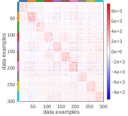
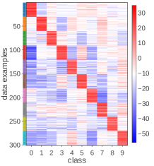
Refer to caption
Refer to caption
(a) MNIST: GP kernel matrix (left) and GP posterior mean (right)
Refer to caption
(b) CIFAR-10: GP posterior mean
Figure 7: This figure visualizes the GP kernel matrix and posterior mean for LeNet5 trained with VOGN on MNIST (left) and CIFAR-10 (right). The kernel matrix clearly shows the correlations learned by the DNN. A higher posterior mean is assigned to the correct label which reflects the accuracy obtained by the DNN.
Refer to caption
(a) Laplace Approximation
Refer to caption
(b) Variational Approximation
Figure 8: GP kernels due to Laplace and variational approximation for neural networks on CIFAR-10. The kernels show slight traces of structure but are not as significant as the ones presented on MNIST in Sec. 5.

C.2 Uncertainties according to DNN2GP for Classification

In this section we present a toy example for the classification task in line with the regression experiment in Fig. 3. We use the reparameterization introduced in App. B.2, in particular Eq. (63). We train a neural network with single hidden layer of 10 units and tanh activation to fit the non-linear decision boundary. We have δ=0.26𝛿0.26\delta=0.26 and train on 100 samples for 5000 full-batch epochs. Fig. 9 shows how the reparameterization allows to decompose predictive variance into label noise due to the decision boundary, see. (b), and model uncertainty, see (c), that grows away from the data.
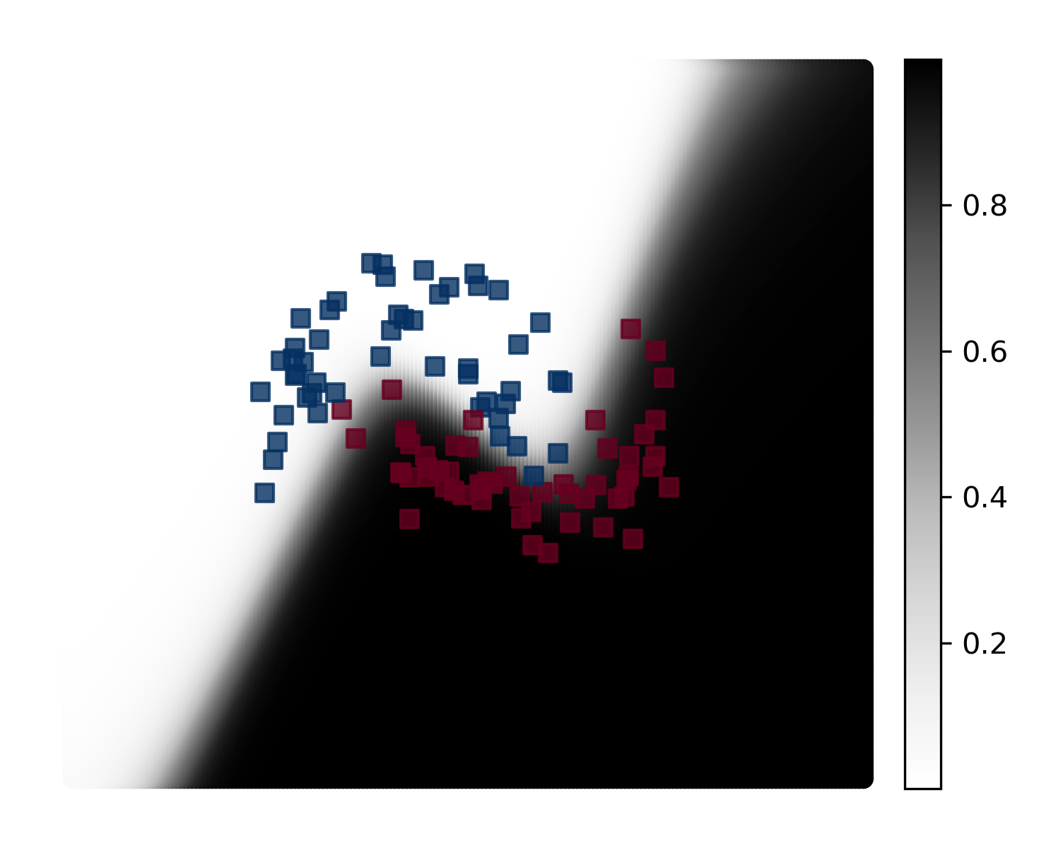
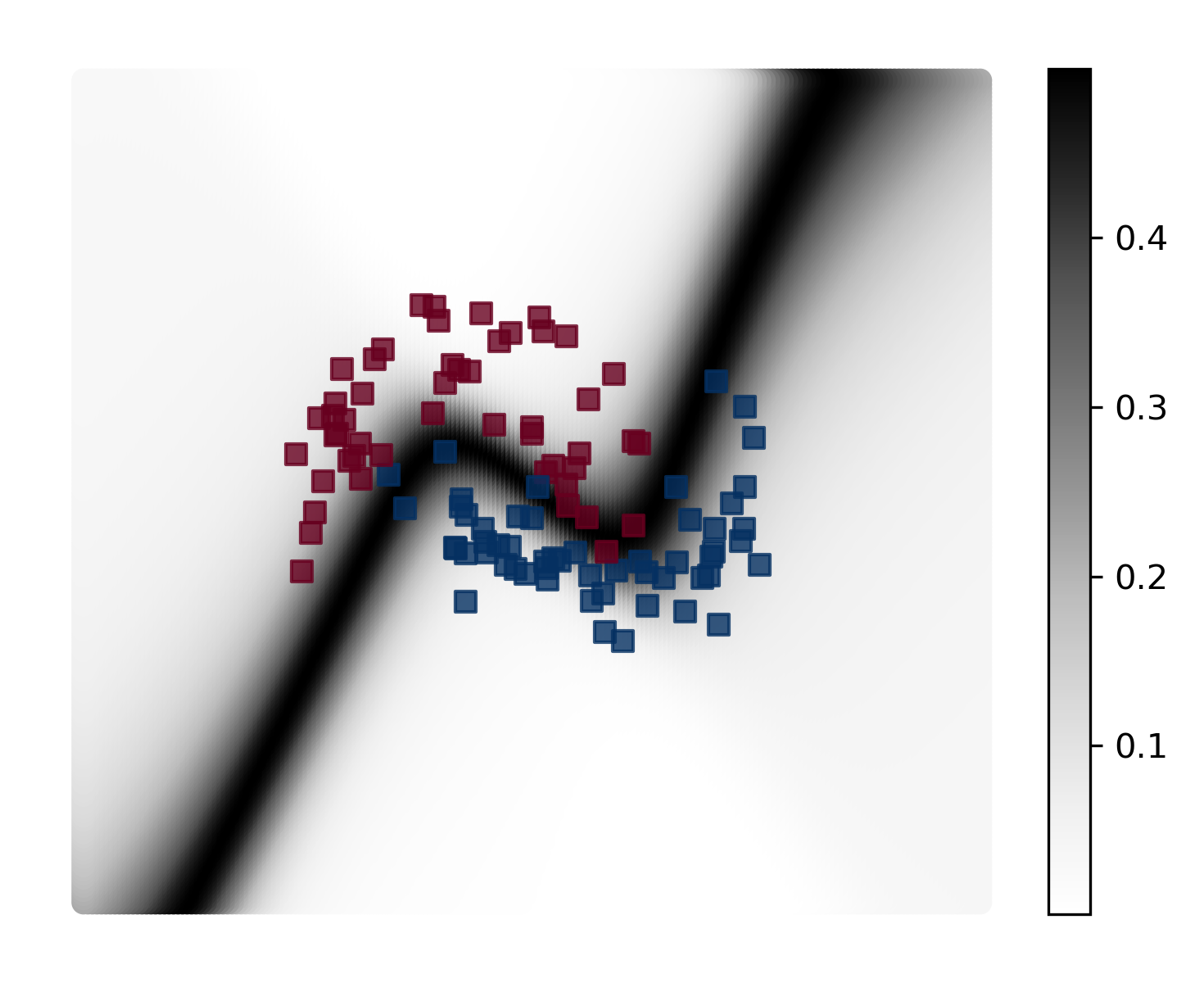
Refer to caption
(c) mean σ(fw(𝐱))𝜎subscript𝑓subscript𝑤subscript𝐱\mbox{$\sigma$}(f_{w_{*}}(\mbox{$\mbox{$\mathbf{x}$}$}_{*}))
Refer to caption
(d) aleatoric uncertainty
Refer to caption
(e) epistemic uncertainty
Figure 9: This figure demonstrates the decomposition of predictive variances due to the reparameterization introduced in App. B.2 on a binary toy classification task (red vs. blue half moons). We plot the quantities of Eq. (63) in figures (a)-(c): (a) is the prediction of a trained NN while the sum of (b) and (c) give us the posterior predictive uncertainties. Around the decision boundary, the label noise (b) is high and remains unchanged further from the data while the predictive uncertainty is low where supported by data and strongly grows away from it. Here, the model fits the data well in contrast to Fig. 4 where the model is unable to do so which results in high estimated label noise.

Appendix D Author Contributions Statement

Author List: Mohammad Emtiyaz Khan, Alexander Immer, Ehsan Abedi, Maciej Korzepa.

M.E.K. conceived a rough idea using the gradients and Hessians of the loss, and wrote the first version of the proofs. A.I. and E.A. made major corrections to M.E.K.’s original version and introduced version used in the final paper. They also came up with the prediction method for DNN2GP. E.A. formalized the NTK connection, and extensively studied its connection to the GP posterior. A.I. did most of the experiments and introduced the necessary reparameterization for applications. M.K. helped on the hyperparameter-tuning experiments, as well as with the visualizations. M.K. did the regression uncertainty experiment with some help from E.A. and A.I.

M.E.K. wrote the main content of the paper. E.A. wrote all the proofs, and A.I. and M.K. summarized the experiment section. All the authors proof-read the paper and revised it.

Appendix E Camera-Ready Version vs the Submitted Version

We made several changes taking reviewers feedback into account.

  1. 1.

    The writing and organization of the papers were modified to emphasize that we are able to relate the iterations of a deep-learning algorithm to GP inference.

  2. 2.

    To improve clarity, Fig. 1 was added as a summary of our approach. The writing was modified to follow Step A, B, and C given in Fig. 1.

  3. 3.

    Titles of Section 3 and 4 were changed to emphasize relationship to "solutions and iterations" of a deep-learning algorithm.

  4. 4.

    Theorem 1 and 2 were simplified to focus only on the posterior of linear model only. Relation to GP is discussed separately.

  5. 5.

    Experiment on GP regression was modified to focus on uncertainty instead of the width of the DNN.

  6. 6.

    Visualization of the GP predictive uncertainty and noise was added on top of predictive mean on CIFAR-10

  7. 7.

    A real-world experiment on Wine dataset was added, where we tune the width of the DNN.