Asymptotic correlation functions in the $\boldsymbol{Q}$-state Potts model:
a universal form for point group $\boldsymbol{C_{4v}}$

Abstract

Reexamining algebraic curves found in the eight-vertex model, we propose an asymptotic form of the correlation functions for off-critical systems possessing rotational and mirror symmetries of the square lattice, i.e., the $C_{4v}$ symmetry. In comparison with the use of the Ornstein-Zernike form, it is efficient to investigate the correlation length with its directional dependence (or anisotropy). We investigate the $Q$-state Potts model on the square lattice. Monte Carlo (MC) simulations are performed using the infinite-size algorithm by Evertz and von der Linden. Fitting the MC data with the asymptotic form above the critical temperature, we reproduce the exact solution of the anisotropic correlation length (ACL) of the Ising model ($Q=2$) within a five-digit accuracy. For $Q=3$ and 4, we obtain numerical evidence that the asymptotic form is applicable to their correlation functions and the ACLs. Furthermore, we successfully apply it to the bond percolation problem which corresponds to the $Q\rightarrow 1$ limit. From the calculated ACLs, the equilibrium crystal shapes (ECSs) are derived via duality and Wulff’s construction. Regarding $Q$ as a continuous variable, we find that the ECS of the $Q$-state Potts model is essentially the same as those of the Ising models on the Union Jack and 4-8 lattices, which are represented in terms of a simple algebraic curve of genus 1.

I INTRODUCTION

For the past few decades, thermal evolution of the equilibrium crystal shape (ECS) Wulff1901 ; Burton1951 has received considerable attention Rottman1981 ; Avron1982 ; Zia1982 ; Beijeren1977 ; Jayaprakash1983 ; Fujimoto1997 ; Fujimoto1992 ; Fujimoto1993 . This revived interest comes from connections between the ECS and the roughening transition phenomena Burton1951 ; Rottman1981 ; Avron1982 ; Zia1982 ; Beijeren1977 ; Jayaprakash1983 . The first exact analysis of the ECS was done for the square-lattice Ising model Rottman1981 ; see also Refs. ​Avron1982 ; Zia1982 .

Here we investigate the square-lattice Potts model Baxter1982 ; Wu1982 . To each site ${\bf r}$ one associates a $Q$-valued variable $q_{\bf r}$. The Hamiltonian is given by

$$E(Q)=-\sum_{\langle{\bf r},{\bf r}^{\prime}\rangle}J_{{\bf r,r}^{\prime}}\delta\left(q_{\bf r},q_{{\bf r}^{\prime}}\right),\quad q_{\bf r}=0,1,\dots,Q-1,$$ (1.1)

where the sum runs over all nearest-neighbor pairs $\langle{\bf r},{\bf r}^{\prime}\rangle$. Note that the $Q=2$ Potts model is equivalent to the Ising model. For general $Q$, the Potts model is exactly solvable at the phase transition point Baxter1982 ; Temperley1971 ; Baxter1973 ; Kluemper1989 ; Buffenoir1993 ; Borgs1992 . The phase transition is continuous for $Q\leq 4$ and first order for $Q>4$.

In a previous study Fujimoto1997 we generalized the argument in Refs. ​Rottman1981 ; Avron1982 ; Zia1982 to find the ECS of the $Q$-state Potts model. We showed that the anisotropic correlation length (ACL) is related by duality Zia1978 ; Laanait1987 ; Holzer1990 ; Akutsu1990 to the anisotropic interfacial tension. For $Q>4$, the ACL was exactly calculated at the first-order transition (or self-dual) point. The ECS was obtained from the ACL via the duality relation and Wulff’s construction Wulff1901 ; Burton1951 . It was expressed as an algebraic curve in the $\alpha\beta$ plane

$$\alpha^{2}\beta^{2}+1+A_{3}(\alpha^{2}+\beta^{2})+A_{4}\alpha\beta=0,$$ (1.2)

where $\alpha=\exp[-\lambda(X+Y)/k_{\rm B}T]$ and $\beta=\exp[-\lambda(X-Y)/k_{\rm B}T]$ with the position vector $(X,Y)$ of a point on the ECS and a suitable scale factor $\lambda$; for definitions of $A_{3}$ and $A_{4}$, see Sec. ​3.2 of Ref. ​Fujimoto1997 . The algebraic curve (1.2) is quite universal because it appears as the ECSs of a wide class of lattice models including the square-lattice Ising model Rottman1981 ; Avron1982 ; Zia1982 ; Beijeren1977 ; Jayaprakash1983 ; Fujimoto1997 ; Fujimoto1992 ; Fujimoto1993 .

We note that Eq. ​(1.2) is not the only universal curve Rutkevich2002 ; Fujimoto2002 . For example, we considered the ACL of the eight-vertex model in Ref. ​Fujimoto1996 and found another algebraic curve

$$\alpha^{2}\beta^{2}+1+{\bar{A}}_{2}(\alpha\beta+1)(\alpha+\beta)+{\bar{A}}_{3}(\alpha^{2}+\beta^{2})+{\bar{A}}_{4}\alpha\beta=0$$ (1.3)

[for definitions of ${\bar{A}}_{2}$, ${\bar{A}}_{3}$, and ${\bar{A}}_{4}$, see Eq. ​(4.7) of Ref. ​Fujimoto1996 ]. The ACL represented by Eq. ​(1.3) is indeed the same as those of the Ising models on the Union Jack and 4-8 lattices Holzer1990a . Some authors derived algebraic curves for the lattice models possessing six-fold rotational symmetry Holzer1990a ; Vaidya1976 ; Zia1986 ; Fujimoto1999 ; Fujimoto1998 ; Fujimoto2002a , which are also universal.

We expect that these algebraic curves are connected with the symmetries of lattice models. How do they select the algebraic curves? This is the problem we shall consider. Also, we expect that the same selection mechanism works regardless of whether the lattice models are exactly solvable or not.

In this paper, we propose an asymptotic form of the correlation functions of off-critical systems possessing rotational and mirror symmetries of the square lattice (the $C_{4v}$ symmetry); see Chap. ​2 of Ref. ​Hamermesh1989 . The asymptotic form is brought about by reexamining exact solutions of the eight-vertex model. We apply it to the $Q$-state Potts model. Our method is a combined use of the asymptotic form and Monte Carlo (MC) simulations based on the Fortuin-Kasteleyn random-cluster representation Fortuin1972 . As we see below, the combined method is quite efficient to calculate the correlation lengths with their anisotropy.

The format of the present paper is as follows: In Sec. ​II, we introduce an asymptotic form for the $C_{4v}$ symmetry, i.e., a form for the asymptotic correlation functions which together with MC data enables us to evaluate the ACLs. In Sec. ​III, we perform MC simulations. We investigate the $Q=2$, 3, and 4 cases, and also the bond percolation model which is, via the cluster representation, realized in the $Q\rightarrow 1$ limit. Sec. ​IV is devoted to discussion and summary. From the evaluated ACL we derive the ECS in the $Q$-state Potts model. Detailed explanations on the exact calculation of the Ising model, the methodology of MC simulations, and the fitting procedure are given in the Appendices.

II ASYMPTOTIC CORRELATION FUNCTIONS FOR $\boldsymbol{C_{4v}}$

Johnson, Krinsky, and McCoy (JKM) Johnson1973 calculated the correlation length of the eight-vertex model along the vertical direction; see also Ref. ​Johnson1972 . Their approach was the row-to-row transfer matrix argument. They investigated the low-lying excitations to determine the next-largest and next-next-largest eigenvalues. In Ref. ​Fujimoto1996 , using the shift operator, we extended the analysis by JKM into general directions; see also Refs. ​Fujimoto1990 ; Fujimoto1990a ; Kluemper1990 .

Because of the symmetry properties of the model, we can restrict ourselves to an antiferroelectric ordered regime (the principal regime) without loss of generality Baxter1982 ; Baxter1973a . It was shown that, for a given parameter $x$ ($0<x<1$), there are two cases with respect to another parameter $q$ (see Fig. ​1) Fujimoto1996 ; for definitions of $x$ and $q$, see Chap. ​10 of Ref. ​Baxter1982 . In the case $0<q<x^{3}$ the ACL is independent of $q$. In the $q\rightarrow x^{4}$ limit the eight-vertex model factors into two square-lattice Ising models. For planar Ising models it was shown that the ECS is determined by the Fourier transform (structure factor) of the asymptotic correlation function Holzer1990 ; Akutsu1990 ; Holzer1990a . In the square-lattice Ising model the inverse of the structure factor above the critical temperature corresponds to the left-hand side of Eq. ​(1.2). We found that for $0<q<x^{3}$ the asymptotic correlation function of the eight-vertex model is related to the algebraic curve (1.2). In the case $x^{3}<q<x^{2}$ the ACL depends on $q$. It was shown that the asymptotic correlation function is connected with Eq. ​(1.3).

Figure 1: A schematic diagram of the principal regime in the eight-vertex model. For a given $x$ $(0<x<1)$, there exist two cases with respect to another parameter $q$: The ACL depends on $q$ for $x^{3}<q<x^{2}$ and does not for $0<q<x^{3}$. The latter region includes the decoupling limit $q=x^{4}$.

The correlation function in the square-lattice Ising model (with ferromagnetic couplings) were investigated by many authors; see, for example, Refs. ​Kadanoff1966 ; Cheng1967 ; McCoy1973 ; Yamada1983 ; Yamada1984 ; Yamada1986 ; Wu1976 ; Camp1971 ; Fisher1971 ; Bariev1975 . The Pfaffian method was used in Ref. ​Cheng1967 ; see also Ref. ​McCoy1973 . Yamada Yamada1983 ; Yamada1984 showed that the results in Ref. ​Cheng1967 coincide with those of the row-to-row transfer matrix. We note that the row direction of the eight-vertex model corresponds to the diagonal direction in the Ising model; transfer matrices of the two models have complex eigenvalues. In the thermodynamic limit, due to their continuous distribution, the summation over the eigenvalues becomes contour integrals. JKM showed that analyticity of the integrand (or eigenvalues) plays an important role: To compare their results in the decoupling limit with those in Ref. ​Cheng1967 , JKM rewrote the latter by the use of elliptic functions, which connect the structure factor with the eigenvalues along the row direction. Then, using the analytic property, they shifted the integration paths suitably to find equivalence between the results along the row and diagonal directions; see Eqs. ​(3.5) and (3.6) in JKM.

In Ref. ​Fujimoto2002 we discussed a close relation between the $C_{4v}$ symmetry and the algebraic curves (1.2) and (1.3). The eight-vertex model was defined on a square lattice rotated through an arbitrary angle with respect to the coordinate axes Fujimoto1994 . Calculating eigenvalues of transfer matrices along various directions, we showed that lattice rotations shift (or deform) the integration paths. We pointed out that, to derive the equivalence between the results by transfer matrices along various directions, two further properties are needed in addition to (i) the analytic property found by JKM: (ii) a functional equation corresponding to the $\pi$-rotational invariance, and (iii) doubly periodic structure. We argued that the properties (i)–(iii) essentially determine the asymptotic form of the correlation function possessing the $C_{4v}$ symmetry.

To ensure the argument in Ref. ​Fujimoto2002 , and to show its applicability to unsolvable models, we consider the $Q$-state Potts model. Since the analysis in Ref. ​Fujimoto2002 was about the correlation function between two arrow spins in the antiferroelectric ordered regime, some ambiguity remained to clarify the role of the $C_{4v}$ symmetry. We successfully applied the same argument as in Ref. ​Fujimoto2002 to the square-lattice Ising model and then found that the properties (i)–(iii) are actually satisfied (see Appendix ​A).

Regarding $Q$ as a continuous variable, we assume (i)–(iii). We estimate the leading asymptotic behavior of the correlation functions for general $Q$ as follows (for clarity here we summarize the discussion given in Appendix ​A.6): The property (iii) shows that, choosing a suitable parametrization, we can represent the asymptotic correlation function ${\cal F}_{{\bf o},{\bf r}}$ as

$${\cal F}_{{\bf o},{\bf r}}=\ {\rm Const.}\int^{\omega_{1}}_{-\omega_{1}}~{}d\Theta~{}{\cal Y}(\Theta)^{j}{\cal X}(\Theta)^{i},$$ (2.1)

with ${\bf r}=i{\bf e}_{x}+j{\bf e}_{y}$. ${\cal Y}(\Theta)$ corresponds to eigenvalues of the row-to-row transfer matrix, and ${\cal X}(\Theta)$ those of the shift operator. Both ${\cal X}(\Theta)$ and ${\cal Y}(\Theta)$ are doubly periodic functions; see Appendix ​A.6.

In the case $Q=2$ the $\pi$ rotation of the lattice corresponds to shifting the integration path by $\omega_{2}$. The property (ii) suggests the relations ${\cal Y}(\Theta+\omega_{2})={\cal Y}(\Theta)^{-1}$ and ${\cal X}(\Theta+\omega_{2})={\cal X}(\Theta)^{-1}$. The property (i) indicates analyticity of ${\cal Y}(\Theta)$ and ${\cal X}(\Theta)$. It follows that ${\cal Y}(\Theta)$ and ${\cal X}(\Theta)$ must be of the form

$${\cal Y}(\Theta)=\prod_{l=1}^{\nu}k^{\frac{1}{2}}{\rm sn}(\Theta+\alpha_{l}),\quad{\cal X}(\Theta)=\prod_{l=1}^{\nu^{\prime}}k^{\frac{1}{2}}{\rm sn}(\Theta+v+\beta_{l}),$$ (2.2)

where $k$ is the modulus corresponding to the modular parameter $\tau=\omega_{2}/\omega_{1}$. When the interactions do not depend on bond directions, the Potts model possesses the fourfold rotational symmetry. We can set $v=\pm\omega_{2}/2$, $\nu=\nu^{\prime}$, and $\alpha_{l}=\beta_{l}$. Since the correlation function is real valued, we find that $\tau$ must be purely imaginary, which ensures the $C_{4v}$ symmetry of the system as well.

It follows from the case $Q=2$ that the simplest form with $\nu=2$ corresponding to the next-largest eigenvalues appears above $T_{\rm C}(Q)$, where we denote the phase transition temperature by $T_{\rm C}(Q)$, regarding it as a function of $Q$. For parameters $\alpha_{1}$ and $\alpha_{2}$, we find two possibilities: $(\alpha_{1}-\alpha_{2})/\omega_{1}$ is purely imaginary or a real number. Since $\alpha_{1}-\alpha_{2}=\omega_{2}/2$ in the case $Q=2$, we assume it is a pure imaginary number. As a result, we obtain for $T>T_{\rm C}(Q)$

$${\cal F}_{{\bf o},{\bf r}}={\rm Const.}\int^{\omega_{1}}_{-\omega_{1}}~{}d\Theta~{}\left[k{\rm sn}(\Theta+B){\rm sn}(\Theta-B)\right]^{j}\left[k{\rm sn}(\Theta+\omega_{2}/2+B){\rm sn}(\Theta+\omega_{2}/2-B)\right]^{i}.$$ (2.3)

Since we cannot determine $\alpha_{1}-\alpha_{2}$ to be $\omega_{2}/2$ solely from the $C_{4v}$ symmetry, we have introduced a parameter $B$. The structure factor of Eq. ​(2.3) is related to the algebraic curve (1.3); we can regard Eq. ​(1.2) is a special limit of Eq. ​(1.3). The asymptotic form (2.3) is expected to be one of general forms for systems possessing the $C_{4v}$ symmetry. The algebraic curve (1.3) is an elliptic curve, i.e., an algebraic curve of genus 1. Eq. ​(2.3) is a differential form on the elliptic curve (1.3) Namba1984 .

As mentioned at the end of Appendix ​A.6, for $T<T_{\rm C}(Q)$ almost the same argument holds: From the case $Q=2$, it follows that $\nu=4$, $\alpha_{1}-\alpha_{2}=\alpha_{3}-\alpha_{4}=\omega_{2}/2$, and $\alpha_{1}-\alpha_{3}$ is a real number. The only difference from the case of $T>T_{\rm C}(Q)$ is expected to be that two elliptic curves are needed to represent the asymptotic correlation function.

III NUMERICAL ANALYSES FOR $\boldsymbol{Q}$-STATE POTTS MODEL

Following the results in Sec. ​II, we investigate the asymptotic correlation functions in the $Q$-state Potts model. For $Q\geq 3$ the phenomena in three or more phase systems have been attracted much attention Selke1982 ; Peczak1989 ; Gupta1992 ; see also Refs. ​Kluemper1989 ; Buffenoir1993 ; Borgs1992 ; Janke1994 ; Janke1997a . In Ref. ​Selke1982 interface properties in $Q=3$ were studied. As mentioned in Sec. ​I, at the first-order transition point, the Potts model possesses the same ACL and ECS as the Ising model Fujimoto1997 . Although for $Q\geq 3$ we expect a deviation of the ECS from the $Q=2$ case, definite results on this subject have not been obtained yet; see, for example, Refs. ​Akutsu1987 ; Akutsu1987a ; Selke1989 .

Also, numerical calculations of the correlation functions and the correlation lengths have been frequently performed. One typical way of doing them is to analyze the exponential decay of correlation function data in a certain fixed direction provided by MC simulations on finite-size systems Janke1994 ; Janke1997a . However, it is recognized that such an approach cannot always give an accurate estimation of the correlation lengths. Further, the present analysis on the ACLs is expected to become more difficult because of the following reasons: First, the finite-size effects in the MC data can affect the analysis of anisotropy in an unexpected manner. Second, because the patterns of the ACLs observed in different models, but sharing the $C_{4v}$ symmetry, are similar to each other Akutsu1987 ; Akutsu1987a , they possess only slight differences (see also Appendix ​B).

In this situation, we employ an algorithm for the MC simulations proposed by Evertz and von der Linden Evertz2001 . Since it is a method for infinite-size systems, an extrapolation of data to the thermodynamic limit is not necessary. For a system in a disordered phase, we generate the random clusters by taking the center site as a seed site and expand the thermally equilibrated area outward (see Appendix ​C). Then, we measure the correlation functions in the area well equilibrated, which are free of the finite-size effects. Typically $O(10^{14})$ random clusters are generated at each temperature to attain the high accuracy of MC data Fortuin1972 .

Our method is a combined use of the MC data with the result in Sec. ​II, which is expected to be quite efficient to investigate the ACLs. In Sec. ​III.1, we shall introduce an asymptotic form for the correlation functions in the $Q$-state Potts model, which includes three parameters. To determine them, fitting calculations are performed for the MC data. In Sec. ​III.2, we calculate the ACL in the $Q=2$ Potts model to demonstrate an accuracy of our numerical analysis. In Sec. ​III.3, we investigate the cases $Q=3$, 4. In Sec. ​III.4 we also apply the method to the bond percolation process corresponding to the $Q\rightarrow 1$ limit.

III.1 A form for asymptotic correlation functions in $\boldsymbol{Q}$-state Potts model

As mentioned at the end of Sec. ​II, since the analysis for $T>T_{\rm C}(Q)$ is more fundamental, we shall restrict ourselves to the case $T>T_{\rm C}(Q)$ below. Suppose a square lattice $\Lambda_{\rm sq}$. We denote the position vector of a site on $\Lambda_{\rm sq}$ as ${\bf r}=i{\bf e}_{x}+j{\bf e}_{y}$. The definition of the correlation function for the $Q$-state Potts model is

$$\left\langle\sigma_{\bf o}\sigma_{\bf r}^{\ast}\right\rangle=\left\langle\exp\left[\frac{2\pi{\rm i}(q_{\bf o}-q_{\bf r})}{Q}\right]\right\rangle=\left\langle\frac{Q\delta\left(q_{\bf o},q_{\bf r}\right)-1}{Q-1}\right\rangle,$$ (3.1)

where $\sigma_{\bf r}=\exp(2\pi{\rm i}q_{\bf r}/Q)$. It was rigorously proven that the correlation function decays exponentially above the transition temperature and at the first-order transition point Wu1982 ; Laanait1987 ; Hintermann1978 .

We shall concentrate on the case of $J_{{\bf r,r}^{\prime}}=2J$, where the transition point is simply given by $k_{\rm B}T_{\rm C}(Q)/J=2/\ln\left(1+\sqrt{Q}\right)$. Based on the observation in Sec. ​II, we shall employ the inferred form in Eq. ​(2.3). The $C_{4v}$ symmetry permits the inclusion of one fitting parameter $B$ other than the elliptic modulus and a normalization factor. We take the Ising model in Appendix ​A as a reference. We replace $\omega_{1}$ and $\omega_{2}$ by $I$ and $I^{\prime}$, respectively. In terms of elliptic functions, our form is rewritten as

$${\cal F}_{\rm sq}(i,j;A,k,b)=\frac{A}{\pi}(1-k^{2})^{\frac{1}{4}}\int^{I}_{-I}d\phi\left[k{\rm sn}(\phi+b\frac{{\rm i}I^{\prime}}{4}){\rm sn}(\phi-b\frac{{\rm i}I^{\prime}}{4})\right]^{j}\left[k{\rm sn}(\phi+(2+b)\frac{{\rm i}I^{\prime}}{4}){\rm sn}(\phi+(2-b)\frac{{\rm i}I^{\prime}}{4})\right]^{i},$$ (3.2)

where $b$ is introduced by $B=b{\rm i}I^{\prime}/4$, and the normalization factor is represented using a parameter $A$; these refer to the exact values $A=1$ and $b=1$ in the $Q=2$ case.

We denote MC data of Eq. ​(3.1) with ${\bf r}=i{\bf e}_{x}+j{\bf e}_{y}\in\Lambda_{\rm sq}$ by $\{c(i,j)\}$. In an asymptotic region of large $R$, we perform a fitting of MC data to determine the three parameters $A$, $k$, $b$. Using the extracted values ${\bar{A}},~{}{\bar{k}},~{}{\bar{b}}$, the asymptotic correlation function is represented as

$$\left\langle\sigma_{\bf o}\sigma_{\bf r}^{\ast}\right\rangle\sim{\cal F}_{\rm sq}(i,j;{\bar{A}},{\bar{k}},{\bar{b}}).$$ (3.3)

We can find the ACL from Eq. ​(3.3) by the method of steepest descent, as shown in Appendix ​A. For example, the inverse correlation length in the diagonal direction is determined as

$$\frac{1}{\xi_{\rm diag}}=-\frac{1}{\sqrt{2}}\ln\left\{\frac{{\rm sn}[I+(1+{\bar{b}})\frac{{\rm i}I^{\prime}}{4}]}{{\rm sn}[I+(3+{\bar{b}})\frac{{\rm i}I^{\prime}}{4}]}\frac{{\rm sn}[I+(1-{\bar{b}})\frac{{\rm i}I^{\prime}}{4}]}{{\rm sn}[I+(3-{\bar{b}})\frac{{\rm i}I^{\prime}}{4}]}\right\}.$$ (3.4)

Note that, when ${\bar{b}}=1$, Eq. ​(3.4) reduces to

$$\frac{1}{\xi_{\rm diag}}=-\frac{1}{\sqrt{2}}\ln{\bar{k}},$$ (3.5)

which coincides with the exact result in $Q=2$. If we succeed in calculating the ACL with a sufficient accuracy, then it gives strong numerical evidence that the elliptic curve (1.3) appears in the structure factor of the asymptotic correlation function.

There are two possible sources of errors in our analysis: One is the statistical errors in $\{c(i,j)\}$, which are inherent in the MC sampling procedures and become larger for longer distances. The other is systematic errors in Eq. ​(3.2). Note that contributions from the eigenvalues with $\nu>2$ are not taken into account in Eq. ​(3.2). They are small corrections to the asymptotic form, but can be important for short distances; see Appendix ​A; although the accuracy of MC data is higher for shorter distances, the fitting results can be worse due to the systematic errors.

We point out that essentially the same situations occur in methods along fixed directions and that these methods are not efficient to control the two kinds of errors; see, for example, Refs. ​Janke1994 ; Janke1997a . On the other hand, for the analysis of ACLs, it is rather natural to fit the MC data in an annular region. We do this with the help of Eq. ​(3.2). We found that, by optimizing a mean radius of the annular region, we can obtain reliable fitting results under a well-controlled condition of two kinds of errors. We provide details of our fittings below and in Appendix ​C.

Figure 2: Annular regions. The origin $(0,0)$ is denoted by the black cell. The annular region ${{\cal D}}(10^{-3},3\times 10^{-4})$ is employed for the fitting of correlation function data of $Q=2$ at $t=0.24$ (308 blue cells). The annulus for $Q=3$ at $t=0.15$ and that for $Q=4$ at $t=0.1$ are indicated by green cells and red cells, respectively. The annulus for $Q=1$ at $t=0.50$ are given by crosses overwritten on the cells.

III.2 $\boldsymbol{Q=2}$ case

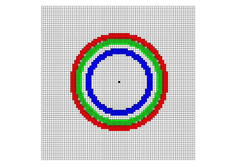
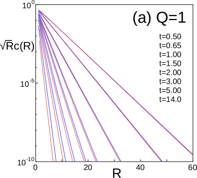
We start with the $Q=2$ Potts model and demonstrate an accuracy of our numerical analysis. We performed extensive MC simulations to achieve a demanded accuracy and fitting the MC data in a suitable annular region. To make it explicit, let us denote an annular region centered at the origin as ${{\cal D}}(c_{\rm max},c_{\rm min})=\{(i,j)|c_{\rm min}<c(i,j)<c_{\rm max}\}$, and the number of included sites as $|{{\cal D}}(c_{\rm max},c_{\rm min})|$. For instance, at the reduced temperature $t=[T-T_{\rm C}(2)]/T_{\rm C}(2)=0.24$, we employed $|{{\cal D}}(10^{-3},3\times 10^{-4})|=308$ with a mean radius $\simeq 16$, as given by blue cells in Fig. ​2. The second column of Table ​1 summarizes the results of $Q=2$. Then, one can find that, at all temperatures $t$, our results coincide with the exact values, $\xi_{\rm exact}$ along the diagonal direction, $A=1$, and $b=1$ within, at least, five-digit accuracy.

As explained in Appendix ​A, the systematic errors for the $Q=2$ Potts model stem from the eigenvalues with $\nu=6$ and $r=-1$, which form the third band, and thus should be smaller than those in other cases. This permits us to use Eq. ​(3.2) for inner annuli. We have checked a very weak dependence of fitting results on radii of inner annuli (see Appendix ​C). In outer regions the statistical errors become larger. However, we have also checked that their accuracy is improved by increasing the MC steps. If we increase the MC steps further, then the same results are expected to appear in outer annuli. Thus, as mentioned at the end of previous section, we can successfully control the two kind of errors, which is the main advantage in our method over calculations based on the Ornstein-Zernike form.

Also, see the second column of Table ​2 and the red lines in Fig. ​3; we can confirm that Eq. ​(3.2) is a quite efficient form of the asymptotic correlation functions, especially, to analyze the correlation lengths with their full anisotropies.

Table 1: The temperature dependence of extracted values of the fitting parameters in Eq. ​(3.2). In addition, the correlation length $\xi_{\rm diag}$ is enumerated; its exact values are given in the $Q=2$ case for comparison. The parenthesized digits indicate errors. The geometries of annular regions employed for fittings are summarized (see text).

$Q$	$t$	$c_{\rm max}$	$c_{\rm min}$	$|{{\cal D}}|$	$\bar{A}$	$\bar{k}$	$\bar{b}$	$\xi_{\rm diag}$	$\xi_{\rm exact}$
1	0.50	$1\times 10^{-4}$	$3\times 10^{-5}$	436	1.024825(6)	0.593506	1.018407(2)	2.750569(1)	n/a
	0.65	$1\times 10^{-4}$	$2\times 10^{-5}$	348	1.018603(5)	0.507724(4)	1.01635(2)	2.113499
	1.00	$1\times 10^{-4}$	$1\times 10^{-5}$	252	1.01061(1)	0.365381(1)	1.012548(5)	1.418417(1)
	1.50	$1\times 10^{-3}$	$1\times 10^{-4}$	104	1.00565	0.245847	1.008724(3)	1.014686(1)
	2.00	$1\times 10^{-3}$	$1\times 10^{-4}$	68	1.00331(1)	0.176466	1.006455	0.819234(1)
	3.00	$1\times 10^{-3}$	$1\times 10^{-4}$	44	1.001351(1)	0.103562	1.003900	0.625435
	5.00	$1\times 10^{-2}$	$1\times 10^{-4}$	36	1.000544(2)	0.0481419	1.001796	0.466765
	14.00	$1\times 10^{-2}$	$1\times 10^{-5}$	32	1.000040(5)	0.00817343(5)	1.000275	0.294259
2	0.24	$1\times 10^{-3}$	$3\times 10^{-4}$	308	1.000006(5)	0.596242(1)	0.999987(7)	2.734823(4)	2.734823
	0.30	$1\times 10^{-2}$	$1\times 10^{-3}$	272	1.000000(3)	0.534544	1.000006	2.257906(2)	2.257906
	0.50	$1\times 10^{-2}$	$1\times 10^{-3}$	132	0.999998(2)	0.386861	1.000001	1.489133	1.489133
	1.00	$1\times 10^{-2}$	$1\times 10^{-3}$	52	0.999996(2)	0.207107	1.000001(7)	0.898187	0.898187
	2.00	$1\times 10^{-1}$	$1\times 10^{-3}$	32	1.000001	0.0888253	1.000000	0.584124	0.584124
	10.00	$1\times 10^{-1}$	$1\times 10^{-4}$	20	0.999999	0.00643374(2)	1.000000	0.280253	0.280253
3	0.15	$1\times 10^{-4}$	$3\times 10^{-5}$	400	0.96856(4)	0.59271(1)	0.98514(7)	2.672979(3)	n/a
	0.20	$1\times 10^{-4}$	$3\times 10^{-5}$	280	0.974811(4)	0.521168(7)	0.98624(2)	2.147209(1)
	0.30	$1\times 10^{-4}$	$1\times 10^{-5}$	284	0.982815(4)	0.414841(6)	0.98813(2)	1.592772(2)
	0.50	$1\times 10^{-4}$	$1\times 10^{-5}$	152	0.99072(3)	0.284116(2)	0.991031(2)	1.116243(5)
	1.00	$1\times 10^{-3}$	$1\times 10^{-4}$	48	0.996832(2)	0.141663	0.995079(2)	0.7210346(1)
	2.00	$1\times 10^{-3}$	$1\times 10^{-5}$	60	0.99923(1)	0.0572655(3)	0.997884	0.493739
	8.00	$1\times 10^{-2}$	$1\times 10^{-5}$	24	0.999977(3)	0.00576756(2)	0.999812	0.2742787(2)
4	0.10	$3\times 10^{-5}$	$1\times 10^{-5}$	428	0.930993(6)	0.59836(1)	0.97189(5)	2.695252(3)	n/a
	0.14	$3\times 10^{-5}$	$1\times 10^{-5}$	264	0.94516(6)	0.522324	0.97424(1)	2.13511(2)
	0.20	$1\times 10^{-4}$	$1\times 10^{-5}$	332	0.95917(3)	0.436457(2)	0.977090(3)	1.67632(1)
	0.30	$1\times 10^{-4}$	$1\times 10^{-5}$	204	0.97308(3)	0.337726(1)	0.980765(2)	1.28399
	0.50	$1\times 10^{-4}$	$1\times 10^{-5}$	100	0.98605(3)	0.223150(3)	0.98580(1)	0.932945(2)
	1.00	$1\times 10^{-4}$	$1\times 10^{-5}$	40	0.995700(8)	0.106277	0.992435(1)	0.627439
	2.00	$1\times 10^{-3}$	$1\times 10^{-5}$	48	0.998968(2)	0.0413266	0.996967	0.4429263(1)
	6.00	$1\times 10^{-2}$	$1\times 10^{-5}$	32	0.999930(4)	0.00668751	0.999560	0.2823396(1)

III.3 $\boldsymbol{Q=3,~{}4}$ cases

In this subsection, we analyze the ACLs observed in the $Q=3$, 4 Potts models by using the same method as in Sec. ​III.2.

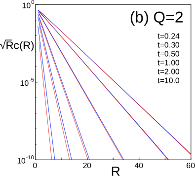
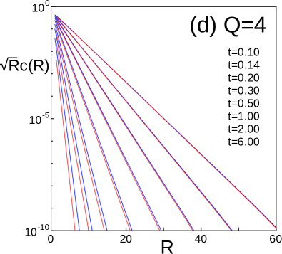
As mentioned in Appendix ​A, the contribution from the next-next largest eigenvalues with $\nu=4$ vanishes due to the ${\mathbb{Z}}_{2}$ symmetry of the $Q=2$ Potts model. We cannot expect the same here. In fact, if we compare the $Q=2$ and $t=0.24$ case with the $Q=3$ and $t=0.15$ case, though values for $\xi_{\rm diag}$ are nearly equal to each other (i.e., $\bar{\xi}\simeq 2.7$), we cannot attain the same accuracy of the fitting for the latter MC data in the former annulus (i.e., blue cells in Fig. ​2). We cannot attribute it to the statistical errors, but to an influence from the contribution of the next-next largest eigenvalues in the latter. Therefore, to circumvent the systematic errors, we need to employ annuli with larger radii than those in the $Q=2$ case. For this issue, we estimate the order of errors included in Eq. ​(3.2) to optimize the annulus employed in the $Q=2$ case. In the $Q=3$ and $t=0.15$ case, denote the deviation at the origin $(0,0)$ as $\Delta(3)$, which is estimated as $\Delta(3)\simeq O(10^{-2})$ (see Appendix ​C). Noting that the next-next largest eigenvalues form the second band, we can estimate their contribution as $\Delta(3)\times{\rm e}^{-2R/\bar{\xi}}$. To obtain the ACL within a sufficient accuracy, we employ $|{{\cal D}}(10^{-4},3\times 10^{-5})|=400$ with the mean radius $\simeq 21$, which is depicted by the green cells in Fig. ​2. The third column of Table ​1 summarizes the results for the $Q=3$ Potts model. We succeeded in fitting the data by Eq. ​(3.2), which permits us to evaluate the ACL of the model within five-digit accuracy at all temperatures calculated. As in the $Q=2$ case, we checked that the improvement of the accuracy was observed for the fitting of data in the outer annuli by increasing MC steps. The obtained results exhibit the relevant deviation from the values of the Ising models.

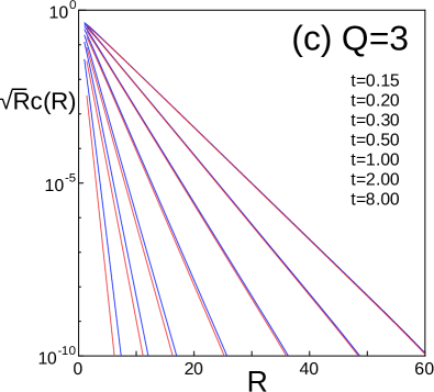
In the $Q=4$ Potts model, the second band contributions become somewhat larger than those in the $Q=3$ case. This can be recognized via the same argument as above: We compare the $Q=3$ and $t=0.15$ case with the $Q=4$ and $t=0.10$ case; the correlation lengths in these cases are nearly equal. We can also estimate the deviation $\Delta(4)$ and then find that it becomes larger than $\Delta(3)$. Therefore, we should employ a slightly larger annulus in radius than corresponding one in the $Q=3$ case. Based on the same order-estimate of the second band contributions as the above, for instance for $t=0.10$, we employed $|{{\cal D}}(3\times 10^{-5},10^{-5})|=428$ with mean radius $\simeq 24$, which is indicated by the red cells in Fig. ​2. The fitting can be performed with the same accuracy as in the $Q=3$ case, and the obtained results are summarized in the fourth column of Table ​1. The deviation from the Ising model becomes more prominent. Note that the parameter $b$ monotonically decreases with the increase of $Q$; we will discuss its physical meanings in Sec. ​IV.

III.4 Bond percolation process as $\boldsymbol{Q\rightarrow 1}$ limit

The Potts model is related to a number of other problems in lattice statistics Baxter1982 ; Wu1982 ; Temperley1971 . These relations make it possible to explore their properties from known results on the Potts model or vice versa Nijs1979 ; Nightingale1980 ; Bloete1982 . The bond percolation provides a simple picture of a phase transition Aharony2003 . Regarding $Q$ as a continuous variable Bloete1982 , we can relate the $Q$-state Potts model to the bond percolation model: Suppose that $Z(Q)$ is the partition function of the $Q$-state Potts model, whose cluster representation is provided in Appendix ​B. Then, the generating function of the bond percolation is given by

$$\lim_{Q\rightarrow 1}\frac{\partial}{\partial Q}\ln Z(Q),$$ (3.6)

where the bond percolation probability is $p=1-{\rm e}^{-2K}$ Baxter1982 , and the percolation threshold $p_{\rm C}$ is $p$ at $T_{\rm C}(1)$. The connectivity function is defined by the probability that the origin ${\bf o}$ and the site ${\bf r}$ belong to the same cluster, and was proven that, for $p<p_{\rm C}$, it decays exponentially as ${\bf r}$ becomes large Higuchi1988 ; Aizenman1987 ; Menshikov1986 . The correlation function (3.1) reduces to the connectivity function in the $Q\rightarrow 1$ limit Wu1982 . Therefore, in this subsection, we investigate the connectivity function in the bond percolation, equivalently the correlation function of the Potts model in the $Q\rightarrow 1$ limit, by using Eq. ​(3.2).

The first column of Table ​1 summarizes the fitting results for $Q=1$. Based on the same argument as above, we optimized the annular regions: for example for $t=0.50$, we employ $|{{\cal D}}(10^{-4},3\times 10^{-5})|=436$ with mean radius $\simeq 22$, which is given by crosses in Fig. ​2. Then, we performed the fittings of the MC data in the optimized annuli to determine $A,~{}k,~{}b$. We obtained the ACL within five-digit accuracy. In the course of fitting calculations, we recognized the systematic errors similarly to the $Q=3$, 4 cases. The extracted parameter values $\bar{A}$ and $\bar{b}$ exhibit deviations from the values of $Q=2$ in the opposite direction to the $Q=3$, 4 cases and reveal their monotonic $Q$ dependence.

As demonstrated, the form (3.2) can accurately fit the asymptotic correlation functions of the $Q=2$, 3, 4 Potts models for $T>T_{\rm C}(Q)$ and the asymptotic connectivity function of the bond percolation ($Q=1$) for $p<p_{\rm C}$. The result strongly suggests that the elliptic curve (1.3) is related to the structure factor for general $Q$. Consequently, we expect that Eq. ​(1.3) plays a key role to describe the asymptotic correlation functions in a wide class of models possessing the $C_{4v}$ symmetry.

IV DISCUSSION AND SUMMARY

We have investigated the asymptotic correlation functions of the $Q$-state Potts model on the square lattice. Revisiting the exact solutions of the eight-vertex model, we pointed out the importance of the three properties of the eigenvalues of the transfer matrix: (i) the analyticity found by JKM Johnson1973 , (ii) the functional equation related to the $\pi$-rotational invariance, and (iii) the doubly periodic structure. Assuming (i)–(iii), we can essentially determine the asymptotic forms with the help of the $C_{4v}$ symmetry.

For the off-critical Ising model $Q=2$ we proved that (i)–(iii) are satisfied; see Appendix ​A. For $Q>4$ the same situation occurs at the first-order transition point. Assuming $Q$ as a continuous variable, we brought the three properties into the asymptotic form with isotropic interactions above the transition temperature as Eq. ​(3.2).

Based on these observations, we have proposed the new approach to analyze the correlation functions by using the result from (i)–(iii) and the numerical procedures combined: Eq. ​(3.2) includes the parameters $A,~{}k,~{}b$ not determined from the $C_{4v}$ symmetry. We performed MC simulations provided by the infinite-size algorithm Evertz2001 , and then carried out fittings of MC data to determine $A,~{}k,~{}b$.

As mentioned in Sec. ​III, there are two types of errors: statistical errors and systematic errors. One typical way of calculating the correlation lengths is to consider the exponential decay of the correlation function along fixed directions, but this method is not efficient to control the two types of errors. We handled these errors successfully by introducing the annular regions for the fitting of $A,~{}k,~{}b$.

To demonstrate the efficiency of our approach, we calculated the ACL of the Ising model above the critical temperature. The obtained results agreed extremely well with the exact values. We investigated the $Q=3$, 4 Potts models for $T>T_{\rm C}(Q)$ and then the bond percolation model (the $Q\to 1$ limit) for $p<p_{\rm C}$. To minimize the errors, the annular regions were optimized carefully. We succeeded in fitting the data within a five-digit accuracy. The high accuracy of the results for $Q=1$, 2, 3, and 4 shows the validity of the asymptotic form (3.2) and that our approach is in fact effective to investigate the ACLs of the system possessing the $C_{4v}$ symmetry.

IV.1 Equilibrium crystal shapes

It was revealed that (I) the structure factors of the $Q$-state Potts model, including the bond percolation as $Q=1$, are represented by the use of the elliptic curve (1.3) and that (II) the parameter $\bar{b}$ monotonically decreases with the increase of $Q$. It is noticeable that, although small in magnitude, (II) provides the reliable evidence of deviation from the case of the Ising model. Here, to show its physical meanings, we investigate the $Q$ dependence of the ECS.

The ECS is the droplet shape of one phase embedded inside a sea of another phase with its volume (or area) fixed Wulff1901 ; Burton1951 ; Rottman1981 ; Avron1982 ; Zia1982 ; Beijeren1977 ; Jayaprakash1983 ; Fujimoto1997 ; Fujimoto1992 ; Fujimoto1993 . Disappearance of facet in the ECS is a signal of the roughening transition Jayaprakash1983 ; Jayaprakash1984 ; Holzer1989 . Once knowing the anisotropic interfacial tension, we can determine the ECS with the help of Wulff’s construction Wulff1901 ; Burton1951 .

In a previous work Fujimoto1997 , we found that for $Q\geq 2$ the ACL is related to the anisotropic interfacial tension as

$$\frac{\gamma^{\ast}}{k_{\rm B}T^{\ast}}=\frac{1}{\xi}\quad{\rm in~{}all~{}directions},$$ (4.1)

where $\gamma^{\ast}$ is the anisotropic interfacial tension at a temperature $T^{\ast}$ [$<T_{\rm C}(Q)$] such that $K^{\ast}=J/k_{\rm B}T^{\ast}$ satisfies the duality condition $({\rm e}^{2K}-1)({\rm e}^{2K^{\ast}}-1)=Q$. We regard $\gamma^{\ast}$ as a function of $\theta_{\perp}$, which is the angle between the normal vector of the interface and ${\bf e}_{x}$-direction; $\theta=\theta_{\perp}+\pi/2$. The ECS is derived from $\gamma^{\ast}(\theta_{\perp})$ with the help of Wulff’s construction as

$$\Lambda{\bf R}=\left(\!\!\begin{array}[]{rr}\cos\theta_{\perp}&-\sin\theta_{\perp}\\ \sin\theta_{\perp}&\cos\theta_{\perp}\end{array}\!\!\right)\left(\!\!\begin{array}[]{c}\gamma^{\ast}(\theta_{\perp})\\ \frac{d\gamma^{\ast}}{d\theta_{\perp}}(\theta_{\perp})\end{array}\!\!\right),$$ (4.2)

where ${\bf R}=(X,Y)$ is the position vector of a point on the ECS and $\Lambda$ a scale factor adjusted to yield the area of the crystal.

Using $\xi$ calculated in Sec. ​III in Eq. ​(4.1), we can derive the ECS via Eq. ​(4.2). Our result is as follows:

$$\Lambda{\bf R}=\left(\!\!\begin{array}[]{c}-\ln\left[{\bar{k}}{\rm sn}(\phi+{\bar{b}}\frac{{\rm i}I^{\prime}}{4}){\rm sn}(\phi-{\bar{b}}\frac{{\rm i}I^{\prime}}{4})\right]\\ -\ln\left[{\bar{k}}{\rm sn}(\phi-(2+{\bar{b}})\frac{{\rm i}I^{\prime}}{4}){\rm sn}(\phi-(2-{\bar{b}})\frac{{\rm i}I^{\prime}}{4})\right]\end{array}\!\!\right)$$ (4.3)

with $\Lambda$ chosen suitably. As $\phi$ moves from 0 to $2{\rm i}I^{\prime}$ on the imaginary axis, ${\bf R}$ sweeps out the ECS. One finds that, reflecting the result (I), the ECS is expressed as Eq. ​(1.3) with $\alpha=\exp(-\Lambda X)$ and $\beta=\exp(-\Lambda Y)$, where ${\bar{A}}_{2}$, ${\bar{A}}_{3}$, ${\bar{A}}_{4}$ are, respectively, given as

$${\bar{A}}_{2}=\frac{2{\rm cn}({\bar{b}}\frac{{\rm i}I^{\prime}}{2}){\rm dn}({\bar{b}}\frac{{\rm i}I^{\prime}}{2})}{1+{\bar{k}}{\rm sn}({\bar{b}}\frac{{\rm i}I^{\prime}}{2})^{2}},~{}{\bar{A}}_{3}=1,~{}{\bar{A}}_{4}=-\frac{({\bar{k}}^{\frac{1}{2}}+{\bar{k}}^{-\frac{1}{2}})^{2}}{1+{\bar{k}}{\rm sn}({\bar{b}}\frac{{\rm i}I^{\prime}}{2})^{2}}.$$ (4.4)

The ECS in the $Q$-state Potts model is the same as those of the Ising models on the Union Jack and 4-8 lattices Holzer1990a .

Table 2: The elliptic modulus dependence of the interfacial tension (4.1) and the radius of the curvature (4.5) in the facet ($\theta_{\perp}=0$) and the corner ($\theta_{\perp}=\frac{\pi}{4}$) directions. The parenthesized digits indicate errors. $t^{\ast}$ denotes a reduced temperature related via the duality condition with $t$.

				$\gamma^{\ast}/k_{\rm B}T^{\ast}$		$\rho/|{\bf R}|$
$Q$	$t$	$t^{\ast}$	$\bar{k}$	$\theta_{\perp}=0$	$\theta_{\perp}=\frac{\pi}{4}$	$\theta_{\perp}=0$	$\theta_{\perp}=\frac{\pi}{4}$
1	0.50	n/a	0.593506	0.362487	0.363561	1.024034	0.976668
	0.65		0.507724(4)	0.470826	0.473149	1.040366(3)	0.961575(3)
	1.00		0.365381(1)	0.697672	0.705011	1.088328(2)	0.920472(1)
	1.50		0.245847	0.966719(1)	0.985527(1)	1.170490(2)	0.859568(1)
	2.00		0.176466	1.186919(2)	1.220652(3)	1.260456	0.803824
	3.00		0.103562	1.530284(5)	1.598887	1.448106(2)	0.713801
	5.00		0.0481419	2.000909	2.142406	1.823115	0.597195
	14.00		0.00817343(5)	3.007556(3)	3.398371(4)	3.361020(8)	0.409052
2	0.24	0.180449	0.596242(1)	0.364650	0.365654	1.022308	0.978298
	0.30	0.212423	0.534544	0.441115	0.442888	1.032748	0.968541
	0.50	0.296641	0.386861	0.665509	0.671532	1.075470	0.931052
	1.00	0.423400	0.207107	1.087883	1.113353	1.209256(1)	0.834354
	2.00	0.542189	0.0888253	1.631399	1.711964	1.506487	0.691295
	10.00	0.726099	0.00643374(2)	3.137726(1)	3.568201(2)	3.666353(8)	0.391270
3	0.15	0.123678	0.59271(1)	0.373113	0.374116	1.021751(7)	0.978826(6)
	0.20	0.155806	0.521168(7)	0.463792	0.465721	1.033903(4)	0.967477(4)
	0.30	0.210524	0.414841(6)	0.623150	0.627836	1.062267(6)	0.942242(5)
	0.50	0.293001	0.284116(2)	0.882588(4)	0.895863(4)	1.129046(3)	0.888962(2)
	1.00	0.416299	0.141663	1.341439	1.386896	1.319586(3)	0.772300(2)
	2.00	0.531350	0.0572655(3)	1.903634(2)	2.025360(3)	1.714394(4)	0.625274(1)
	8.00	0.692933	0.00576756(2)	3.197038(3)	3.645926(3)	3.815002(3)	0.383675
4	0.10	0.087335	0.59836(1)	0.370106	0.371023	1.020045(5)	0.980445(5)
	0.14	0.116378	0.522324	0.466507(3)	0.468359(3)	1.032331(2)	0.968928(1)
	0.20	0.155063	0.436457(2)	0.592715(4)	0.596544(4)	1.053238	0.950094
	0.30	0.209177	0.337726(1)	0.770348(4)	0.778821(4)	1.092567	0.917077
	0.50	0.290435	0.223150(3)	1.050345(4)	1.071875(3)	1.18063(1)	0.85286(1)
	1.00	0.411331	0.106277	1.528807(2)	1.593782(2)	1.419833(4)	0.725893(2)
	2.00	0.523800	0.0413266	2.100168	2.257712	1.898554	0.580533
	6.00	0.656712	0.00668751	3.118181(2)	3.541834(2)	3.609079(2)	0.394535

Figure 3: Elliptic modulus dependence of interfacial tension and radius of curvature in the facet ($\theta_{\perp}=0$) and the corner ($\theta_{\perp}=\frac{\pi}{4}$) directions. The correspondence between marks and $Q$ is provided in (a); the fitting curves are a guide for the eye. The figures plot the data normalized by the corresponding values of $Q=2$, which are calculated for an extracted $\bar{k}$ by taking $\bar{b}=1$ in Eqs. ​(4.1) and (4.5). The bare Ising values are also given by numerals (see Table ​2).

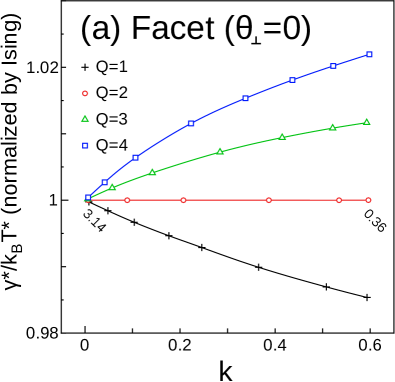
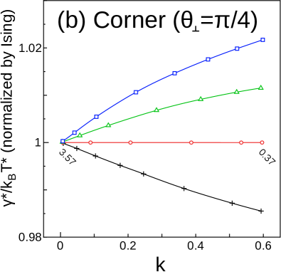
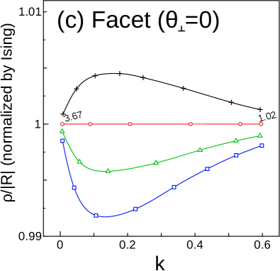
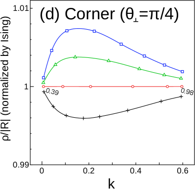
Note that, for a given $\theta_{\perp}$, $\gamma^{\ast}/k_{\rm B}T^{\ast}$ (or the inverse correlation length $1/\xi$) is a function of $k$ and $Q$. From (II), it follows that with the increase of $Q$ but keeping $k$ fixed $\gamma^{\ast}/k_{\rm B}T^{\ast}$ becomes larger in all directions. It is helpful to calculate the radius of curvature $\rho$. The row and the diagonal directions are particularly important in connection with the roughening transition phenomena: In the zero temperature limit, we expect that the ECS is a square, and that a facet and a corner appear at $\theta_{\perp}=0$ and $\pi/4$, respectively. Since $\Lambda{\bf R}=\gamma^{\ast}(\cos\theta_{\perp},\sin\theta_{\perp})$ in these directions, it follows that

$$\frac{\rho}{|{\bf R}|}=\left(1+\frac{1}{\gamma^{\ast}}\frac{d^{2}\gamma^{\ast}}{d{\theta_{\perp}}^{2}}\right),\quad\theta_{\perp}=0,~{}\pi/4.$$ (4.5)

We can proffer the numerical data of $\gamma^{\ast}/k_{\rm B}T^{\ast}$ and $\rho/|{\bf R}|$ at $\theta_{\perp}=0$ and $\pi/$4. We summarize the results in Table ​2, which indicates that, for a given $k$, the ECS deforms slightly to a more circular shape as $Q$ increases.

The deformation is small: Up to a few percentages in curvature. To make it visible, we normalize the bare data using the corresponding values of $Q=2$ Rottman1981 ; Avron1982 . In Fig. ​3, the data normalized by the corresponding exact values are plotted. Figs. ​3(a) and 3(b) show that, as $Q$ increases (with $k$ fixed), $\gamma^{\ast}/k_{\rm B}T^{\ast}$ becomes larger in both directions. From Figs. ​3(c) and 3(d), we find that the radius of the curvature becomes smaller at $\theta_{\perp}=0$, and larger at $\theta_{\perp}=\pi/4$, which means that the ECS of the $Q$-state Potts model becomes slightly rounded in the facet direction and simultaneously flatter in the corner direction. Consequently, the ECS deforms monotonically to a more circular shape as $Q$ increases (see, for example, Fig. ​4 of Ref. ​Fujimoto1996 or Fig. ​3 of Ref. ​Holzer1990a ).

The $Q$ dependence of the shape can be extended into $Q\geq 1$ with the ECS replaced by the polar plot of $1/\xi$. The results obtained here is somewhat unusual: In typical cases, as the correlation length of the system becomes larger, the ECS or the polar plot of $1/\xi$ more circular. One should note that the unusual situation also occurs in the eight-vertex model Fujimoto1996 and the Ising models on the Union Jack and 4-8 lattices Holzer1990 .

In the eight-vertex model, continuously varying exponents can be explained by the weak universality concept Suzuki1974 , where the inverse correlation length $1/\xi$ is regarded as a variable measuring departure from criticality. Our results imply that the elliptic modulus $k$ describing the ACL is more essential than $1/\xi$. That is, even if they have different values of $1/\xi$, the models sharing the same value of $k$ are the same in the amount of the deviation from the critical point. We suggest a possibility that the algebraic geometry provides the birational equivalence Namba1984 as a framework to denote this kind of equivalence. Note that the algebraic curve (1.3) is a singular curve possessing two nodes at infinity, and the algebraic geometry offers a standard procedure to treat such curves. One scenario is that the weak universality concept is connected with the birational equivalence between algebraic curves like Eq. ​(1.3). It is expected that the connection to the algebraic geometry will break a new ground in the study of statistical models.

IV.2 Universal asymptotic forms

Before the analyses of the eight-vertex model, we commonly observed the curves like Eq. ​(1.3) as the ECSs of the various models solved by the Pfaffian method and that the curves can be related to the three properties (i)–(iii); see Secs. ​I and II, and references therein. In Ref. ​Holzer1990a it was also shown that the ECSs like Eq. ​(1.3) do not survive for the modified KDP model because its excitations exhibit a unidimensional band structure and explicitly break the double periodicity condition. These imply that the universality of Eq. ​(1.3) and the applicability of Eq. ​(3.2) are connected with rather generic properties than a specific solvability condition.

Further, the three properties are expected to be robust against some continuous variations of lattice models. For the $Q$-state Potts model, by MC simulations, we confirmed that Eq. ​(3.2) can indeed fit the numerical data of asymptotic correlation functions with high accuracy. This indicates that the universality of our form (3.2) emerges via the robustness of the three properties (i)–(iii).

Further investigations on this subject are desirable. We expect that Eq. ​(3.2) or (2.3) is a universal form for the asymptotic correlation functions with the $C_{4v}$ symmetry. While the $Q$-state Potts model possesses discrete variables, an investigation of continuous spin models, like the classical XY model, is important to clarify the degree of applicability of Eq. ​(3.2). In this paper, we have restricted ourselves to the models defined on the square lattice. It is natural to expect that the same argument is applicable to other lattices, e.g., a triangular, a honeycomb, and so on. Thus, modifications of Eq. ​(3.2) for other point groups, e.g., $C_{6v}$ are interesting Holzer1990a ; Vaidya1976 ; Zia1986 ; Fujimoto1999 ; Fujimoto1998 ; Fujimoto2002a ; see also Refs. ​Jayaprakash1984 ; Holzer1989 . At last, our investigations may include an application of the present form to the problems such as the susceptibility calculations containing higher-order terms Yamada1986 ; Chan2011 . We will report our studies on these topics in the future.

Appendix A EXACT CALCULATION OF CORRELATION LENGTH IN SQUARE-LATTICE ISING MODEL

In Chap. ​7 of Ref. ​Baxter1982 Baxter exactly calculated the correlation length of the square-lattice Ising model along the diagonal direction. We extend the transfer matrix argument into all directions using the shift operator. In order to find the role of the $C_{4v}$ symmetry, we consider the Ising model on a rotated square lattice.

A.1 Commuting transfer matrices in $\boldsymbol{Q=2}$

Suppose a square lattice drawn diagonally. For each site ${\bf r}=i{\bf e}_{x}+j{\bf e}_{y}$ we introduce a variable $\sigma_{\bf r}$, which is related to the $Q$-valued variable $q_{\bf r}$ in Eq. ​(1.1) as $\sigma_{\bf r}=\exp(2\pi{\rm i}q_{\bf r}/Q)$. When $Q=2$, $\sigma_{\bf r}=\pm 1$ and $\delta\left(q_{\bf r},q_{{\bf r}^{\prime}}\right)=\frac{1}{2}(1+\sigma_{\bf r}\sigma_{{\bf r}^{\prime}})$. Thus, the $Q=2$ Potts model (with $J_{{\bf r,r}^{\prime}}$ replaced by $2J_{{\bf r,r}^{\prime}}$) is equivalent to the Ising model whose Hamiltonian is given by

$$E=-\sum_{\bf r}\left(J\sigma_{{\bf r}+{\bf e}_{x}}\sigma_{\bf r}+J^{\prime}\sigma_{{\bf r}+{\bf e}_{y}}\sigma_{\bf r}\right).$$ (A1)

The nearest-neighbor spins are coupled by $J$ or $J^{\prime}$ depending on the direction. We assume $J$, $J^{\prime}>0$. The partition function is

$$Z=\sum_{\sigma}\exp\left[\sum_{\bf r}\left(K\sigma_{{\bf r}+{\bf e}_{x}}\sigma_{\bf r}+K^{\prime}\sigma_{{\bf r}+{\bf e}_{y}}\sigma_{\bf r}\right)\right],$$ (A2)

where the outer sum is over all spin configurations and the reduced couplings $K=J/k_{\rm B}T$ and $K^{\prime}=J^{\prime}/k_{\rm B}T$.

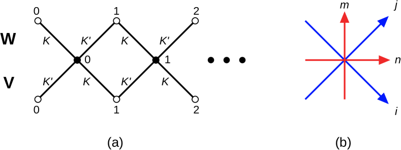
We introduce diagonal-to-diagonal transfer matrices: Consider two successive rows, and let $\sigma=\{\sigma_{0},\dots,\sigma_{N-1}\}$ (respectively, $\sigma^{\prime}=\{\sigma_{0}^{\prime},\dots,\sigma_{N-1}^{\prime}\}$) be the spins in the lower (respectively, upper) row. We assume the periodic boundary conditions in both directions. Then, as shown in Fig. ​4(a), the transfer matrices ${\bf V}$ and ${\bf W}$ are defined by elements as

$$[{\bf V}]_{\sigma,\sigma^{\prime}} =\exp\left[\sum_{l=0}^{N-1}(K\sigma_{l+1}\sigma_{l}^{\prime}+K^{\prime}\sigma_{l}\sigma_{l}^{\prime})\right],$$ (A3)

$$[{\bf W}]_{\sigma,\sigma^{\prime}} =\exp\left[\sum_{l=0}^{N-1}(K\sigma_{l}\sigma_{l}^{\prime}+K^{\prime}\sigma_{l}\sigma_{l+1}^{\prime})\right],$$ (A4)

where $\sigma_{N}=\sigma_{0}$ and $\sigma_{N}^{\prime}=\sigma_{0}^{\prime}$ (see Chap. ​7 of Ref. ​Baxter1982 ). When the system has $2M$ rows, the partition function is given as follows:

$$Z={\rm Tr}{\bf U}^{M}=\sum_{p=0}^{2^{N}-1}\left(\Lambda_{p}^{2}\right)^{M},\qquad{\bf U}={\bf VW},$$ (A5)

where $\Lambda_{p}^{2}$ is the $p$th eigenvalue of ${\bf U}$.

Figure 4: (a) Three successive rows of the square lattice drawn diagonally. (b) The transfer matrix ${\bf U}$ operates spins on a row to transfer them from lower to upper direction along the $m$-axis. The $i$ and $j$ axes correspond to the directions of the primitive translation vectors ${\bf e}_{x}$ and ${\bf e}_{y}$ of the square lattice, respectively.

Above the critical temperature $T_{\rm C}$, we parametrize $K$ and $K^{\prime}$ using the elliptic functions with the modulus $k\in(0,1)$ as

$$\sinh 2K=\frac{k{\rm sn}({\rm i}u)}{{\rm i}},\quad\cosh 2K={\rm dn}({\rm i}u),$$ (A6)

$$\sinh 2K^{\prime}=\frac{{\rm i}}{{\rm sn}({\rm i}u)},\quad\cosh 2K^{\prime}={\rm i}\frac{{\rm cn}({\rm i}u)}{{\rm sn}({\rm i}u)}.$$ (A7)

The quarter periods are denoted by $I$ and $I^{\prime}$; and the argument $u$ satisfies the condition $0<u<I^{\prime}$ (see also Chap. ​15 of Ref. ​Baxter1982 and Ref. ​Baxter1978 ). For $T<T_{\rm C}$, we find the similar parametrization:

$$\sinh 2K=\frac{{\rm sn}({\rm i}u)}{{\rm i}},\quad\cosh 2K={\rm cn}({\rm i}u),$$ (A8)

$$\sinh 2K^{\prime}=\frac{{\rm i}}{k{\rm sn}({\rm i}u)},\quad\cosh 2K^{\prime}={\rm i}\frac{{\rm dn}({\rm i}u)}{k{\rm sn}({\rm i}u)}.$$ (A9)

Regard $k$ as a fixed constant, and $u$ as a complex variable. Then ${\bf U}$ is a function of $u$. When we write it as ${\bf U}(u)$, it satisfies the commutation relation

$$[{\bf U}(u),{\bf U}(u^{\prime})]=0\quad\forall u,u^{\prime}\in\mathbb{C}.$$ (A10)

Further, it commutes with the matrix ${\bf R}$ defined by elements as

$$[{\bf R}]_{\sigma,\sigma^{\prime}}=\prod_{l=0}^{N-1}\delta(\sigma_{l},-\sigma_{l}^{\prime}),$$ (A11)

i.e.,

$$[{\bf U}(u),{\bf R}]=0.$$ (A12)

For simplicity, suppose that $N$ is an even number, then it follows that $\Lambda(u)$ is a doubly periodic function of $u$:

$$\Lambda(u+2I^{\prime})=r\Lambda(u),~{}\Lambda(u-2{\rm i}I)=r\Lambda(u)\text{~{}for~{}}T>T_{\rm C},$$ (A13)

$$\Lambda(u+2I^{\prime})=r\Lambda(u),~{}\Lambda(u-2{\rm i}I)=\Lambda(u)\text{~{}for~{}}T<T_{\rm C},$$ (A14)

where $r$ ($=\pm 1$) is the eigenvalue of ${\bf R}$ corresponding to $\Lambda(u)$. In addition, it is found that

$$\Lambda(u)\Lambda(u+I^{\prime})$$ (A15)

$$=(-2)^{N}\Bigl{\{}\frac{1}{{\rm sn}({\rm i}u)^{N}}+\left[k{\rm sn}({\rm i}u)\right]^{N}r\Bigr{\}}\text{~{}for~{}}T>T_{\rm C},$$ (A16)

$$=(-2)^{N}\Bigl{\{}\frac{1}{[k{\rm sn}({\rm i}u)]^{N}}+{\rm sn}({\rm i}u)^{N}r\Bigr{\}}\text{~{}for~{}}T<T_{\rm C}.$$ (A17)

To determine explicit forms of $\Lambda(u)$, we can use Eq. ​(A16) with the periodicity (A13) for $T>T_{\rm C}$, and Eq. ​(A17) with Eq. ​(A14) for $T<T_{\rm C}$. For example, it is shown that the maximum eigenvalue $\Lambda_{0}(u)^{2}$ behaves as $\Lambda_{0}(u)^{2}\sim\kappa(u)^{2N}$, when $N$ becomes large, and the per-site free energy $f$ is given by

$$- \frac{f}{k_{\rm B}T}=\ln\kappa(u)=$$ (A18)

$$\frac{1}{2\pi}\int_{0}^{\pi}d\theta\ln\left\{2\left[\cosh 2K\cosh 2K^{\prime}+c(\theta)\right]\right\},\quad$$ (A19)

where

$$c(\theta) =\left(1-2k^{+1}\cos 2\theta+k^{+2}\right)^{\frac{1}{2}}\text{~{}~{}for~{}~{}}T>T_{\rm C},$$ (A20)

$$=\left(1-2k^{-1}\cos 2\theta+k^{-2}\right)^{\frac{1}{2}}\text{~{}~{}for~{}~{}}T<T_{\rm C}$$ (A21)

(see Sec. ​7.9 of Ref. ​Baxter1982 ).

A.2 Shift operator method

In Chap. ​7 of Ref. ​Baxter1982 Baxter analyzed the asymptotic behavior of the correlation function using ${\bf U}(u)$. The correlation length was exactly calculated along the diagonal direction. We can extend the calculation into all directions with the help of the shift operator ${\bf S}$, which moves spins on a row along horizontal direction, i.e.,

$$[{\bf S}]_{\sigma,\sigma^{\prime}}=\prod_{l=0}^{N-1}\delta(\sigma_{l},\sigma_{l+1}^{\prime}).$$ (A22)

Let ${\bf r^{+}}$ be the position vector of a site on the sublattice containing the origin ${\bf o}$; we start with choosing two sites on the same sublattice, but this restriction will be removed later. In the usual transfer matrix method the expectation value of the spin product $\sigma_{\bf o}\sigma_{{\bf r}^{+}}$ is represented as

$$\left\langle\sigma_{\bf o}\sigma_{{\bf r}^{+}}\right\rangle=\frac{{\rm Tr}[{\bf A}_{0}{\bf U}^{m}{\bf A}_{n}{\bf U}^{M-m}]}{{\rm Tr}{\bf U}^{M}},$$ (A23)

$$~{}~{}{{\bf r}^{+}}=n({\bf e}_{x}+{\bf e}_{y})+m(-{\bf e}_{x}+{\bf e}_{y})$$ (A24)

where ${\bf A}_{k}$s are defined by

$$[{\bf A}_{k}]_{\sigma,\sigma^{\prime}}=\sigma_{k}\prod_{l=0}^{N-1}\delta(\sigma_{l},\sigma_{l}^{\prime}).$$ (A25)

Apply a similarity transformation to diagonalize ${\bf U}$. We take the $M\rightarrow\infty$ limit first, then the $N\rightarrow\infty$ limit. In the $M\rightarrow\infty$ limit, we find that

$$\left\langle\sigma_{\bf o}\sigma_{{\bf r}^{+}}\right\rangle=\sum_{p}[{\tilde{\bf A}}_{0}]_{0,p}[{\tilde{\bf A}}_{n}]_{p,0}\left[\frac{\Lambda_{p}(u)}{\Lambda_{0}(u)}\right]^{2m},$$ (A26)

where $\Lambda_{p}(u)^{2}$ is the $p$th eigenvalue of ${\bf U}(u)$ in decreasing order of magnitude, and ${\tilde{\bf A}}_{k}$ is the matrix transformed from ${\bf A}_{k}$. Equation ​(A26) implies that the ratios between the eigenvalues of ${\bf U}(u)$ essentially determine the asymptotic behavior of the correlation function along the diagonal direction. For example, when $n$ is fixed and $m$ becomes large, the correlation length along the diagonal direction is calculated from the ratios between $\Lambda_{0}(u)^{2}$ and the next-largest eigenvalues.

To find the asymptotic form in all directions, we consider the anisotropic correlation length (ACL), which is obtainable by taking the $m\rightarrow\infty$ limit with the ratio $n/m$ fixed to be constant. In this limit contribution from the matrix elements $[{\tilde{\bf A}}_{0}]_{0,p}$ and $[{\tilde{\bf A}}_{n}]_{p,0}$ is important as well as the ratios between the eigenvalues. This causes a difficulty since the direct calculation of the matrix elements is very complicated in most cases.

We can overcome the difficulty with the help of the shift operator ${\bf S}$ Fujimoto1990 ; Fujimoto1990a ; Kluemper1990 ; see also Refs. ​Yamada1983 ; Yamada1984 . Because the shift operator relates ${\bf A}_{n}$ to ${\bf A}_{0}$ as

$${\bf A}_{n}={\bf S}^{-n}{\bf A}_{0}{\bf S}^{n},$$ (A27)

we rewrite Eq. ​(A26) as

$$\left\langle\sigma_{\bf o}\sigma_{{\bf r}^{+}}\right\rangle=\sum_{p}[{\tilde{\bf A}}_{0}]_{0,p}[{\tilde{\bf A}}_{0}]_{p,0}\left[\frac{\Lambda_{p}(u)}{\Lambda_{0}(u)}\left({\frac{S_{p}}{S_{0}}}\right)^{\frac{\gamma}{2}}\right]^{2m}$$ (A28)

with

$$\gamma=-\frac{n}{m},$$ (A29)

where $S_{p}$ is the $p$th eigenvalue of ${\bf S}$ and $S_{0}=1$. Eq. ​(A28) shows that we can obtain the ACL from the eigenvalues of ${\bf U}(u)$ and those of ${\bf S}$ without calculating the matrix elements.

A.3 Limiting function $\boldsymbol{L(u)}$

To consider the $N\rightarrow\infty$ limit, we define limiting functions as

$$L_{p}(u)=\lim_{N\rightarrow\infty}\frac{\Lambda_{p}(u)}{\kappa(u)^{N}},\quad p=0,1,\dots,$$ (A30)

where $\kappa(u)$ is given by Eqs. ​(A19)–(A21); note that $L_{0}(u)\equiv 1$. It is shown that

$$\frac{S_{p}}{S_{0}}=\lim_{u\rightarrow 0}L_{p}(u)^{2}.$$ (A31)

From Eqs. ​(A28), (A30), and (A31), we obtain

$$\left\langle\sigma_{\bf o}\sigma_{{\bf r}^{+}}\right\rangle=\sum_{p}[{\tilde{\bf A}}_{0}]_{0,p}[{\tilde{\bf A}}_{0}]_{p,0}\left[L_{p}(u)L_{p}(0)^{\gamma}\right]^{2m}.$$ (A32)

Using Eqs. ​(A13)–(A21), we can determine the form of $L(u)$. When $N$ becomes large and $-I^{\prime}/2<\Re(u)<I^{\prime}/2$, the first term is dominant on the right-hand side of Eq. ​(A16). We keep only the dominant term there Kluemper1990 . Divide the both sides by $\kappa(u)^{N}\kappa(u+I^{\prime})^{N}$ and use Eqs. ​(A19), (A20), and (A30). Combining the result from the second equation of (A13), we find that

$$L(u)L(u+I^{\prime})=1,~{}L(u-2{\rm i}I)=rL(u)\text{~{}for~{}}T>T_{\rm C}.$$ (A33)

Similarly, from Eq. ​(A17) and the second equation of (A14), we obtain

$$L(u)L(u+I^{\prime})=1,~{}L(u-2{\rm i}I)=L(u)\text{~{}for~{}}T<T_{\rm C}.$$ (A34)

Because the zeros of $\Lambda_{0}(u)$ are located on the line $\Re(u)=-I^{\prime}/2$ in a periodic rectangle, the first equation of (A33) or (A34) shows that the limiting function is written as

$$L(u)=F(u)\prod_{l=1}^{\nu}\frac{a-xa_{l}}{a-x^{3}a_{l}},~{}~{}-\frac{I^{\prime}}{2}<\Re(u)\leq\frac{3I^{\prime}}{2}$$ (A35)

with $a=\exp\left(-{\pi u}/{I}\right)$, $a_{l}=\exp\left({{\rm i}\pi\phi_{l}}/{I}\right)$, and $x=\exp\left(-{\pi I^{\prime}}/{2I}\right)$. A function $F(u)$ is analytic and nonzero for $-I^{\prime}/2<\Re(u)\leq 3I^{\prime}/2$. Thus, the limiting functions are labeled by an integer $\nu$ and real numbers $\phi_{1},\phi_{2},\dots,\phi_{\nu}$ instead of $p$.

Substitute Eq. ​(A35) into the first equation of (A33) or (A34), take the logarithms of both sides, and then expand them in the annulus $-I^{\prime}/2<\Re(u)<I^{\prime}/2$ using the form

$$\ln F(u)=c_{0}+ \alpha\ln a+\sum_{\mu=1}^{\infty}\left(c_{\mu}a^{\mu}+c_{-\mu}a^{-\mu}\right),$$ (A36)

$$-\frac{I^{\prime}}{2}<\Re(u)\leq\frac{3I^{\prime}}{2}.$$ (A37)

Equating coefficients gives

$$c_{0}=-\frac{1}{2}\sum_{l=1}^{\nu}\ln(-a_{l}),~{}\alpha=\frac{\nu}{2},~{}c_{\mu}=\frac{x^{\mu}}{1+x^{2\mu}}\frac{1}{\mu}\sum_{l=1}^{\nu}a_{l}^{-\mu},$$ (A38)

$$c_{-\mu}=-\frac{x^{3\mu}}{1+x^{-2\mu}}\frac{1}{\mu}\sum_{l=1}^{\nu}a_{l}^{\mu}$$ (A39)

with $\mu=1,2,\dots$. We find that

$$L(u)=\pm\prod_{l=1}^{\nu}k^{\frac{1}{2}}{\rm sn}({\rm i}u-\phi_{l}-\frac{{\rm i}I^{\prime}}{2}),~{}~{}-\frac{I^{\prime}}{2}<\Re(u)\leq\frac{3I^{\prime}}{2}.$$ (A40)

For $T>T_{\rm C}$, from the second equation of (A33), it follows that $\nu$ is an odd (even) integer if $r=-1$ ($r=+1$). The next-largest eigenvalues correspond to the case with $\nu=1$ and $r=-1$.

For $T<T_{\rm C}$, the two largest eigenvalues $\Lambda_{0}(u)^{2}$ and $\Lambda_{1}(u)^{2}$ are asymptotically degenerate when $N$ becomes large. Note that $r=+1$ for $\Lambda_{0}(u)^{2}$ and $r=-1$ for $\Lambda_{1}(u)^{2}$ (see Sec. ​7.10 of Ref. ​Baxter1982 ). The second equation of (A34) shows that $\nu$ is an even number. We thus find that the next-largest eigenvalues correspond to the cases with $\nu=2$ and $r=\pm 1$.

A.4 Anisotropic correlation lengths $\boldsymbol{Q=2}$

It is shown that, because of continuous distributions of eigenvalues, the sum in Eq. ​(A28) becomes integrals over $\phi_{l}$s in the $N\rightarrow\infty$ limit Johnson1973 . For simplicity, we choose the positive sign in Eq. ​(A40). Detailed analysis also shows that the maximum eigenvalue $\Lambda_{0}(u)^{2}$ corresponds to the case $r_{0}=+1$, and $[{\tilde{\bf A}}_{0}]_{0,p}$ and $[{\tilde{\bf A}}_{0}]_{p,0}$ vanish unless $r_{p}=-1$ due to the ${\mathbb{Z}}_{2}$ symmetry of the system, where $r_{p}$ is the $p$th eigenvalue of ${\bf R}$.

For $T>T_{\rm C}$, only the band of next-largest eigenvalues with $\nu=1$ and $r=-1$ contributes to the leading asymptotic behavior of the correlation function in the limit of $m$ large with $\gamma$ fixed. It follows that

$$\left\langle\sigma_{\bf o}\sigma_{{\bf r}^{+}}\right\rangle-\left\langle\sigma_{\bf o}\right\rangle\left\langle\sigma_{{\bf r}^{+}}\right\rangle\sim\int^{I}_{-I}d\phi\rho(\phi)\left\{k^{\frac{1}{2}}{\rm sn}({\rm i}u-\phi-\frac{{\rm i}I^{\prime}}{2})\left[k^{\frac{1}{2}}{\rm sn}(-\phi-\frac{{\rm i}I^{\prime}}{2})\right]^{\gamma}\right\}^{2m},$$ (A41)

where the function $\rho(\phi)$ is to be determined from the distribution of eigenvalues, and matrix elements $[{\tilde{\bf A}}_{0}]_{0,p}$, $[{\tilde{\bf A}}_{0}]_{p,0}$. Because $r=+1$ for eigenvalues with $\nu=2$, $[{\tilde{\bf A}}_{0}]_{0,p}$ and $[{\tilde{\bf A}}_{0}]_{p,0}$ vanish. Therefore, the first correction to the asymptotic behavior (A41) comes from the integral over the band of eigenvalues with $\nu=3$ and $r=-1$ Yamada1984 .

As stated in Appendix ​A.2, we extend the above analysis to include any pair of sites. Because ${\bf r}^{+}=(n-m){\bf e}_{x}+(n+m){\bf e}_{y}$ [see Fig. ​4(b)], we obtain the transformation of the coordinates, i.e.,

$$i=n-m,\qquad j=n+m.$$ (A42)

We can remove the restriction $i\pm j={\rm even}$ in Eq. ​(A41) to find the correlation function for all ${\bf r}$ as

$$\left\langle\sigma_{\bf o}\sigma_{\bf r}\right\rangle-\left\langle\sigma_{\bf o}\right\rangle\left\langle\sigma_{\bf r}\right\rangle\sim\int^{I}_{-I}d\phi\rho(\phi)\left\{k{\rm sn}({\rm i}u-\phi-\frac{{\rm i}I^{\prime}}{2}){\rm sn}(-\phi+\frac{{\rm i}I^{\prime}}{2})\left[k{\rm sn}({\rm i}u-\phi+\frac{{\rm i}I^{\prime}}{2}){\rm sn}(-\phi+\frac{{\rm i}I^{\prime}}{2})\right]^{\Gamma}\right\}^{j},$$ (A43)

where $\Gamma$ is the ratio given by

$$\Gamma=\frac{i}{j}=\frac{\gamma+1}{\gamma-1}.$$ (A44)

Along the direction designated by $\Gamma$, the correlation length $\xi$ is defined as

$$-\frac{1}{\xi}=\lim_{R\rightarrow\infty}\frac{\ln\left[\left\langle\sigma_{\bf o}\sigma_{\bf r}\right\rangle-\left\langle\sigma_{\bf o}\right\rangle\left\langle\sigma_{\bf r}\right\rangle\right]}{R},\quad R=\sqrt{i^{2}+j^{2}},$$ (A45)

where the limit is taken with $\Gamma$ fixed. We regard $\xi$ as a function of $\theta$, the angle between ${\bf e}_{x}$ and the direction of $\Gamma$. Explicitly, $\Gamma$ is related to $\theta$ as

$$\Gamma=\frac{1}{\tan\theta},\quad\frac{\pi}{4}<\theta<\frac{5\pi}{4}.$$ (A46)

We assume an analyticity of $\rho(\phi)$ and then estimate the integral on the right-hand side of Eq. ​(A43) by the method of steepest descent. It follows that

$$-\frac{1}{\xi} =\sin\theta\ln\left[k{\rm sn}({\rm i}u-\phi_{\rm s}-\frac{{\rm i}I^{\prime}}{2}){\rm sn}(-\phi_{\rm s}+\frac{{\rm i}I^{\prime}}{2})\right]$$ (A47)

$$+\cos\theta\ln\left[k{\rm sn}({\rm i}u-\phi_{\rm s}+\frac{{\rm i}I^{\prime}}{2}){\rm sn}(-\phi_{\rm s}+\frac{{\rm i}I^{\prime}}{2})\right],$$ (A48)

where the saddle point $\phi_{\rm s}$ is determined as a function of $\theta$ by

$$\sin\theta\frac{d}{d\phi_{\rm s}}\ln\left[k{\rm sn}({\rm i}u-\phi_{\rm s}-\frac{{\rm i}I^{\prime}}{2}){\rm sn}(-\phi_{\rm s}+\frac{{\rm i}I^{\prime}}{2})\right]+$$ (A49)

$$\cos\theta\frac{d}{d\phi_{\rm s}}\ln\left[k{\rm sn}({\rm i}u-\phi_{\rm s}+\frac{{\rm i}I^{\prime}}{2}){\rm sn}(-\phi_{\rm s}+\frac{{\rm i}I^{\prime}}{2})\right]=0$$ (A50)

with the condition $\phi_{\rm s}={\rm i}u-{{\rm i}I^{\prime}}/{2}\pm I$ for $\theta={3\pi}/{4}$. The relation $\xi(\theta+\pi)=\xi(\theta)$ implies that the result in Eqs. ​(A48) and (A50) is analytically continued into $0<\theta<2\pi$. Note that increasing $\theta$ by $2\pi$ causes $\Im(\phi_{\rm s})$ to decrease by $2I^{\prime}$. We expect that $\rho(\phi)$ is a doubly periodic function and is analytic inside and on a periodic rectangle. According to Liouville’s theorem, it should be a constant.

Shifting the integration path along the imaginary axis, we can rewrite Eq. ​(A43) as

$$\left\langle\sigma_{\bf o}\sigma_{\bf r}\right\rangle-\left\langle\sigma_{\bf o}\right\rangle\left\langle\sigma_{\bf r}\right\rangle\sim\text{Const}$$ (A51)

$$\times\oint\frac{d\alpha}{\alpha}\oint\frac{d\beta}{\beta}\frac{\alpha^{i}\beta^{j}}{2a-\gamma_{1}(\alpha+\alpha^{-1})-\gamma_{2}(\beta+\beta^{-1})},\qquad$$ (A52)

where contours of integrations are unit circles, and

$$a=(1+z_{1}^{2})(1+z_{2}^{2}),\quad\gamma_{1}=2z_{2}(1-z_{1}^{2}),\quad\gamma_{2}=2z_{1}(1-z_{2}^{2})$$ (A53)

with $z_{1}=\tanh K$ and $z_{2}=\tanh K^{\prime}$. We note that Eqs. ​(A52) and (A53) coincide with the results in Sec. ​4 of Ref. ​Cheng1967 and Sec. ​XII-4 of Ref. ​McCoy1973 ; see also Ref. ​Yamada1984 . In the case of the isotropic interactions the denominator of the integrand has the same form as that in a special case of the left-hand side of Eq. ​(1.3). Therefore, it follows that the structure factor of the asymptotic correlation function possesses the same algebraic property as that of the eight-vertex model.

For $T<T_{\rm C}$, because the band of next-largest eigenvalues with $\nu=2$ and $r=-1$ determines the leading asymptotic behavior of the correlation function. We obtain

$$\left\langle\sigma_{\bf o}\sigma_{{\bf r}^{+}}\right\rangle-\left\langle\sigma_{\bf o}\right\rangle\left\langle\sigma_{{\bf r}^{+}}\right\rangle\sim\int^{I}_{-I}d\phi_{1}\int^{I}_{-I}d\phi_{2}\rho(\phi_{1},\phi_{2}) \left\{k^{\frac{1}{2}}{\rm sn}({\rm i}u-\phi_{1}-\frac{{\rm i}I^{\prime}}{2})\left[k^{\frac{1}{2}}{\rm sn}(-\phi_{1}-\frac{{\rm i}I^{\prime}}{2})\right]^{\gamma}\right\}^{2m}$$ (A54)

$$\times \left\{k^{\frac{1}{2}}{\rm sn}({\rm i}u-\phi_{2}-\frac{{\rm i}I^{\prime}}{2})\left[k^{\frac{1}{2}}{\rm sn}(-\phi_{2}-\frac{{\rm i}I^{\prime}}{2})\right]^{\gamma}\right\}^{2m}.$$ (A55)

Again, the function $\rho(\phi_{1},\phi_{2})$ is to be calculated from the distribution of eigenvalues and the matrix elements $[{\tilde{\bf A}}_{0}]_{0,p}$, $[{\tilde{\bf A}}_{0}]_{p,0}$. Assume an analyticity of $\rho(\phi_{1},\phi_{2})$ and integrate by steepest descents. Then, we find that the correlation length $\xi^{\ast}$ below $T_{\rm C}$ is related to $\xi$ above $T_{\rm C}$ determined by Eqs. ​(A48) and (A50) as

$$\xi=2\xi^{\ast}\quad\text{in all directions}.$$ (A56)

Shifting the integration paths suitably, we find that Eq. ​(A55) is essentially the same as the leading asymptotic form in Sec. ​3 of Ref. ​Cheng1967 and Sec. ​XII-3 of Ref. ​McCoy1973 . The asymptotic correlation function is expressed in terms of the differential forms on the same algebraic curve as in Eq. ​(A52). The difference from the case $T>T_{\rm C}$ is that two elliptic curves are needed in the case $T<T_{\rm C}$.

A.5 Passive rotations

In Ref. ​Yamada1984 it was shown that the results of the correlation functions by the Pfaffian method in Refs. ​McCoy1973 ; Cheng1967 are equivalent to those by the row-to-row transfer matrix. The analyses in the previous section suggest that difference in direction along which the transfer matrix is defined causes a shift or deformation of the integration paths in the asymptotic correlation function. To clarify this point, we apply the argument for the eight-vertex model in Ref. ​Fujimoto2002 to the square-lattice Ising model.

The method given in Appendix ​A.2 corresponds to the active rotations. We employ another method corresponding to the passive rotations: We define the Ising model on a square lattice rotated through an arbitrary angle with respect to the coordinate axes. The rotated system is related to an inhomogeneous system possessing a one-parameter family of commuting transfer matrices. A product of commuting transfer matrices can be interpreted as a transfer matrix acting on zigzag walls in the rotated system Fujimoto2002 ; Fujimoto1994 .

For convenience, we denote the Boltzmann weight of four edges as

$$W(a,b|c,d|u)=2\cosh(K^{\prime}a+Kb+K^{\prime}c+Kd),$$ (A57)

where $a$, $b$, $c$, and $d$ are the nearest-neighbor spins of $f$ arranged as in Fig. ​5. Note that $K$, $K^{\prime}$ are given by Eq. ​(A7) for $T>T_{\rm C}$ and by Eq. ​(A9) for $T<T_{\rm C}$.

Figure 5: The Boltzmann weight of four edges $W(a,b|c,d|u)$, where $a$, $b$, $c$, and $d$ are the nearest-neighbor spins of $f$ summed.

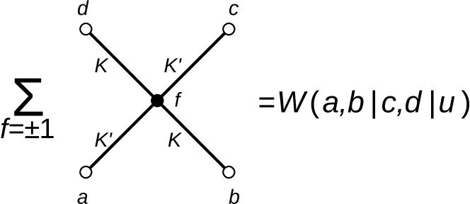
The weight $W(a,b|c,d|u)$ satisfies the following properties Fujimoto1994 , i.e., the standard initial condition

$$\lim_{u\rightarrow 0}\frac{W(a,b|c,d|u)}{\kappa(u)^{2}}=\delta(a,c),$$ (A58)

and the crossing symmetry

$$W(a,b|c,d|I^{\prime}-u)=W(b,a|d,c|u),$$ (A59)

where $\kappa(u)$ is given by Eqs. ​(A19)–(A21). Since $\kappa(I^{\prime}-u)=\kappa(u)$, it follows from Eqs. ​(A58) and (A59) that

$$\lim_{u\rightarrow I^{\prime}}\frac{W(a,b|c,d|u)}{\kappa(u)^{2}}=\delta(b,d).$$ (A60)

To calculate $\xi$ along the direction $\theta$, we consider the Ising model on a square lattice rotated through $3\pi/4-\theta$ with respect to the one drawn diagonally. Let $\sigma=\{\sigma_{0},\dots,\sigma_{N-1}\}$ (respectively, $\sigma^{\prime}=\{\sigma_{0}^{\prime},\dots,\sigma_{N-1}^{\prime}\}$) be the spins on the lower (respectively, upper) row of open circles shown in Fig. ​4(a). Suppose that $N=(|n|+m)N_{0}$, where $m>0$ and $N_{0}$ is an even number. Then, we define inhomogeneous transfer matrices as

$$[{\bf U}_{\rm IH}(u)]_{\sigma,\sigma^{\prime}}=\prod_{l=0}^{N_{0}-1}\left[\prod_{s=l(|n|+m)}^{l(|n|+m)+|n|-1}\!\!\!\!\!\!W(\sigma_{s},\sigma_{s+1}|\sigma_{s+1}^{\prime},\sigma_{s}^{\prime}|u)\!\!\!\prod_{t=l(|n|+m)+|n|}^{(l+1)(|n|+m)-1}\!\!\!\!\!\!W(\sigma_{t},\sigma_{t+1}|\sigma_{t+1}^{\prime},\sigma_{t}^{\prime}|u+u_{0}-H(-n)I^{\prime})\right]$$ (A61)

with $\sigma_{N}=\sigma_{0}$ and $\sigma_{N}^{\prime}=\sigma_{0}^{\prime}$, where $0<u_{0}<I^{\prime}$ and $H(\cdot)$ is the Heaviside step function.

The commutation relation (A10) is generalized as

$$[{\bf U}_{\rm IH}(u),{\bf U}_{\rm IH}(u^{\prime})]=0\quad\forall u,u^{\prime}\in\mathbb{C},$$ (A62)

and (A12) as

$$[{\bf U}_{\rm IH}(u),{\bf R}]=0.$$ (A63)

By using ${\bf U}_{\rm IH}(u)$, we can construct a transfer matrix ${\bar{\bf U}}$ acting on zigzag walls in the rotated system as

$$\bar{\bf U}=\left[\lim_{u\rightarrow 0}\frac{{\bf U}_{\rm IH}(u)}{\kappa(u)^{2|n|N_{0}}}\right]^{m}\left[\lim_{u\rightarrow I^{\prime}-u_{0}}\frac{{\bf U}_{\rm IH}(u)}{\kappa(u+u_{0})^{2mN_{0}}}\right]^{|n|}\qquad \text{~{}for~{}}n>0,$$ (A64)

$$=\left[\lim_{u\rightarrow I^{\prime}}\frac{{\bf U}_{\rm IH}(u)}{\kappa(u)^{2|n|N_{0}}}\right]^{m}\left[\lim_{u\rightarrow I^{\prime}-u_{0}}\frac{{\bf U}_{\rm IH}(u)}{\kappa(u+u_{0}-I^{\prime})^{2mN_{0}}}\right]^{|n|} \text{~{}for~{}}n\leq 0,$$ (A65)

where $n$ and $m$ are related to $\theta$ by $n/m=\tan(3\pi/4-\theta)$ with $\pi/4<\theta<5\pi/4$ (see Fig. ​2 of Ref. ​Fujimoto1994 ). ${\bar{\bf U}}$ reduces to the diagonal-to-diagonal transfer matrix in the case $n=0$, and to the row-to-row transfer matrix in the case $n=m$ (or $n=-m$). We can find the correlation length along any direction of $\theta$ from the eigenvalues of ${\bar{\bf U}}$.

Noting the relations

$$\sum_{f}W(a,b|f,d|u)W(f,b|c,d|-u)=-(2\sinh 2K^{\prime})^{2}\delta(a,c),$$ (A66)

$$\sum_{f}W(a,b|f,d|u-I^{\prime})W(f,b|c,d|-u+I^{\prime})=-(2\sinh 2K)^{2}\delta(a,c)$$ (A67)

with $\sinh 2K$, $\sinh 2K^{\prime}$ given by Eq. ​(A7) or (A9), we also construct a shift operator ${\bar{\bf S}}$ as

$$\bar{\bf S}=\left[-\lim_{u\rightarrow-u_{0}}(2\sinh 2K^{\prime})^{2}\right]^{-|n|mN_{0}}\left[\lim_{u\rightarrow-u_{0}}\frac{{\bf U}_{\rm IH}(u)}{\kappa(u+u_{0})^{2mN_{0}}}\right]^{m}\left[\lim_{u\rightarrow 0}\frac{{\bf U}_{\rm IH}(u)}{\kappa(u)^{2|n|N_{0}}}\right]^{|n|}\qquad~{} \text{~{}for~{}}n>0,$$ (A68)

$$=\left[-\lim_{u\rightarrow-u_{0}}(2\sinh 2K)^{2}\right]^{-|n|mN_{0}}\left[\lim_{u\rightarrow I^{\prime}-u_{0}}\frac{{\bf U}_{\rm IH}(u)}{\kappa(u+u_{0}-I^{\prime})^{2mN_{0}}}\right]^{m}\left[\lim_{u\rightarrow 0}\frac{{\bf U}_{\rm IH}(u)}{\kappa(u)^{2|n|N_{0}}}\right]^{|n|} \text{~{}for~{}}n\leq 0.$$ (A69)

We denote eigenvalues of ${\bf U}_{\rm IH}(u)$ as $\Lambda_{\rm IH}(u)^{2}$. When $N_{0}$ (or $N$) becomes large with $n$ and $m$ fixed, the maximum eigenvalue $\Lambda_{\rm IH;0}(u)^{2}$ behaves as

$$\Lambda_{\rm IH;0}(u)^{2}\sim\kappa(u)^{2|n|N_{0}}\kappa(u+u_{0}-H(-n)I^{\prime})^{2mN_{0}},$$ (A70)

where $\kappa(u)$ is given by Eqs. ​(A19)–(A21) Baxter1978 . We introduce the limiting function as

$$L_{\rm IH}(u)=\lim_{N_{0}\rightarrow\infty}\frac{\Lambda_{\rm IH}(u)}{\kappa(u)^{2|n|N_{0}}\kappa(u+u_{0}-H(-n)I^{\prime})^{2mN_{0}}}.$$ (A71)

The expectation value of $\sigma_{\bf o}\sigma_{{\bf r}^{+}}$ is represented as

$$\left\langle\sigma_{\bf o}\sigma_{{\bf r}^{+}}\right\rangle=\sum_{p}[{\bar{\bf A}}_{0}]_{0,p}[{\bar{\bf A}}_{0}]_{p,0}\times$$ (A72)

$$\qquad L_{{\rm IH};p}(-H(-n)I^{\prime})^{2m}L_{{\rm IH};p}(I^{\prime}-u_{0})^{2|n|},$$ (A73)

where ${\bar{\bf A}}_{0}$ is the matrix transformed from ${\bf A}_{0}$ in Eq. ​(A25) by a similarity transformation to diagonalize ${\bf U}_{\rm IH}(u)$. Almost the same argument as in Appendix ​A.3 yields that $L_{\rm IH}(u)$ must be of the form

$$L_{\rm IH}(u)=\pm\prod_{l=1}^{\nu}k^{\frac{1}{2}}{\rm sn}({\rm i}u-{\bar{\phi}}_{l}-\frac{{\rm i}I^{\prime}}{2}),$$ (A74)

where ${\bar{\phi}}_{l}$s are complex numbers determined by the condition that the eigenvalues of the shift operator ${\bar{\bf S}}$ are unimodular, i.e.,

$$\left|L_{\rm IH}(-u_{0})^{m}L_{\rm IH}(0)^{n}\right|=1.$$ (A75)

From Eqs. ​(A74) and (A75), we can reproduce the asymptotic behavior of the correlation function found in Appendix ​A.4, i.e., Eq. ​(A41) or (A43) for $T>T_{\rm C}$ and Eq. ​(A55) for $T<T_{\rm C}$.

Now, we consider the correlation function for $T>T_{\rm C}$ (almost the same argument holds for $T<T_{\rm C}$). The asymptotic correlation function is given as follows:

$$\left\langle\sigma_{\bf o}\sigma_{{\bf r}^{+}}\right\rangle-\left\langle\sigma_{\bf o}\right\rangle\left\langle\sigma_{{\bf r}^{+}}\right\rangle\sim\int_{C}d{\bar{\phi}}{\bar{\rho}}({\bar{\phi}})\left[k^{\frac{1}{2}}{\rm sn}(-{\bar{\phi}}-\frac{{\rm i}I^{\prime}}{2})\right]^{2m}\left[k^{\frac{1}{2}}{\rm sn}(-{\rm i}u_{0}-{\bar{\phi}}+\frac{{\rm i}I^{\prime}}{2})\right]^{2n}.$$ (A76)

Note that the contour $C$ is determined by the condition (A75), and the rotations of the lattice deform $C$. For instance, in the case $n=0$ ($\theta=3\pi/4$), $\int_{C}$ denotes an integral over a period interval of the length $2I$ on the line $\Im[{\bar{\phi}}]=-u_{0}$, where Eq. ​(A76) reduces to Eq. ​(A41) by the relations ${\bar{\phi}}=\phi-{\rm i}u_{0}$ and ${\bar{\rho}}({\bar{\phi}})=\rho(\phi)$ with $u_{0}$ replaced by $u$. In the case $n=m$ ($\theta=\pi/2$), the contour $C$ is on the line $\Im[{\bar{\phi}}]=-u_{0}/2$. The equivalence between Eqs. ​(A41) and (A76) is derived with the help of the analyticity of the integrand. Using the deformation of $C$, we can extend the result in Eqs. ​(A43)–(A50) into all directions.

The $\pi$ rotation of the lattice corresponds to shifting the integration paths by ${\rm i}I^{\prime}$ in Eq. ​(A76), which is connected with the fact that the twofold rotational symmetry of the system appears with the help of the relation

$$k^{\frac{1}{2}}{\rm sn}({\bar{\phi}}\pm{\rm i}I^{\prime})=\left[k^{\frac{1}{2}}{\rm sn}({\bar{\phi}})\right]^{-1}.$$ (A77)

In the case of isotropic interactions, where $u_{0}=I^{\prime}/2$, the $\pi/2$ rotation causes a shift of the integration paths by ${\rm i}I^{\prime}/2$, which relates the eigenvalues of ${\bar{\bf U}}$ to those of $\bar{\bf S}$.

A.6 Asymptotic form for general $\boldsymbol{Q}$

The results by transfer matrices along various directions should be equivalent. It is pointed out that this equivalence is derived with the help of analytic properties of the integrand; see the integrand in the right-hand side of Eq. ​(A43), and also Ref. ​Johnson1973 . Therefore, (i) analyticity of the integrands is needed to ensure the equivalence between the results along various directions. Two further properties are pointed out: From the fact that increasing $\theta$ by $\pi$ causes $C$ to shift by $-{\rm i}I^{\prime}$ along the imaginary axis, it follows that the twofold rotational symmetry is directly connected with the relation (A77). We find that (ii) the same relation as (A77) is satisfied by the limiting functions; see the first equation of (A33) or (A34). Note that Eqs. ​(1.2) and (1.3) represent elliptic curves (i.e., they are algebraic curves of genus 1) Namba1984 . We find that (iii) the asymptotic correlation function is written in terms of elliptic functions (or differential forms on a Riemann surface of genus 1).

The meaning of (iii) can be explained as follows: Two-dimensional (2D) lattice models are related to 2D Euclidean field theories in their critical limit and for distances much larger than the lattice spacing. For a Euclidean field, the dispersion relation is written as $p_{x}^{2}+p_{y}^{2}+m^{2}=0$ with a suitable mass term $m$, and the correlation function has a periodic structure describing the rotational symmetry. For off-critical lattice models, two kinds of periodicity appear: One is connected with two-, four-, or sixfold rotational symmetry, and the other with the fact that eigenvalues of the transfer matrix are periodic functions of crystal momentum. This doubly periodic structure leads to the property (iii).

Assuming (i)–(iii), we can essentially determine the leading asymptotic behavior of the correlation functions with the $C_{4v}$ symmetry. The property (iii) shows that, choosing a suitable parametrization, we can write the correlation function as

$$\left\langle\sigma_{\bf o}\sigma_{\bf r}\right\rangle-\left\langle\sigma_{\bf o}\right\rangle\left\langle\sigma_{\bf r}\right\rangle\sim\ {\rm Const.}\int^{\omega_{1}}_{-\omega_{1}}~{}d\Theta~{}{\cal Y}(\Theta)^{j}{\cal X}(\Theta)^{i},$$ (A78)

where ${\cal Y}(\Theta)$ comes from eigenvalues of the row-to-row transfer matrix, and ${\cal X}(\Theta)$ the corresponding ones of the shift operator; ${\cal X}(\Theta)$ and ${\cal Y}(\Theta)$ are doubly periodic: ${\cal X}(\Theta+2\omega_{1})={\cal X}(\Theta+2\omega_{2})={\cal X}(\Theta)$ and ${\cal Y}(\Theta+2\omega_{1})={\cal Y}(\Theta+2\omega_{2})={\cal Y}(\Theta)$. The property (ii) yields the relations ${\cal Y}(\Theta+\omega_{2})={\cal Y}(\Theta)^{-1}$ and ${\cal X}(\Theta+\omega_{2})={\cal X}(\Theta)^{-1}$, and the property (i) indicates analyticity of ${\cal Y}(\Theta)$ and ${\cal X}(\Theta)$. As a result, ${\cal Y}(\Theta)$ and ${\cal X}(\Theta)$ must be of the forms

$${\cal Y}(\Theta)=\prod_{l=1}^{\nu}k^{\frac{1}{2}}{\rm sn}(\Theta+\alpha_{l}),\quad{\cal X}(\Theta)=\prod_{l=1}^{\nu^{\prime}}k^{\frac{1}{2}}{\rm sn}(\Theta+v+\beta_{l}).$$ (A79)

In the case $K=K^{\prime}$ ($J=J^{\prime}$) the present Ising model possesses the fourfold rotational symmetry. We can set $v=\pm\omega_{2}/2$, $\nu=\nu^{\prime}$, and $\alpha_{l}=\beta_{l}$. Since the correlation function is real valued, we find that the modular parameter $\tau=\omega_{2}/\omega_{1}$ must be pure imaginary, which ensure the $C_{4v}$ symmetry of the system as well. It follows from Eq. ​(A43) that the simplest case $\nu=2$ appears for $T>T_{\rm C}$. For parameters $\alpha_{1}$ and $\alpha_{2}$, we find two possibilities: $(\alpha_{1}-\alpha_{2})/\omega_{1}$ is purely imaginary or a real number; $\alpha_{1}-\alpha_{2}=\omega_{2}/2$ gives Eq. ​(A43) with $u=I^{\prime}/2$. The results are closely related to the $C_{4v}$ symmetry except that $\alpha_{1}-\alpha_{2}=\omega_{2}/2$. We expect that Eq. ​(A43) is applicable with the relation $\alpha_{1}-\alpha_{2}=\omega_{2}/2$ modified suitably for general $Q$ and $T>T_{\rm C}(Q)$.

Almost the same argument holds for $T<T_{\rm C}(Q)$: It follows that $\nu=4$, $\alpha_{1}-\alpha_{2}=\alpha_{3}-\alpha_{4}=\omega_{2}/2$, and $\alpha_{1}-\alpha_{3}$ is a real number. As mentioned above, the only difference from the case of $T>T_{\rm C}(Q)$ is that two elliptic curves are needed to represent the asymptotic correlation function (see Sec. ​3 of Ref. ​Cheng1967 and Sec. ​XII-3 of Ref. ​McCoy1973 ).

Appendix B DETAILS OF MONTE CARLO SIMULATIONS FOR INFINITE-SIZE SYSTEMS

We perform large-scale MC simulations to investigate the correlation functions. In this Appendix, we shall detail our methodology. The Hamiltonian of the square-lattice $Q$-state Potts model is given by Eq. ​(1.1). We treat it in the case of $J_{{\bf r,r}^{\prime}}=2J$. According to Fortuin and Kasteleyn (FK) Fortuin1972 , the random-cluster representation of the partition function is given as

$$Z(Q) ={\rm Tr}{\rm e}^{-E(Q)/k_{\rm B}T}$$ (B1)

$$=\sum_{\{n\}}p^{\sum_{{\bf r}^{\ast}}n_{{\bf r}^{\ast}}}(1-p)^{\sum_{{\bf r}^{\ast}}(1-n_{{\bf r}^{\ast}})}Q^{N_{\rm c}},$$ (B2)

where $p=1-{\rm e}^{-2K}$ is the bond percolation probability. $n_{{\bf r}^{\ast}}=0,1$ is the bond occupation defined for ${\bf r}^{\ast}\in\Lambda^{*}_{\rm sq}$, and $\Lambda^{*}_{\rm sq}$ is the medial lattice of $\Lambda_{\rm sq}$. We denoted the number of FK clusters as $N_{\rm c}$. While there are some variations in implementations of cluster MC simulations Swendsen1987 ; Wolff1988 ; Wolff1989 ; Evertz2001 , we employ the so-called infinite-size method proposed by Evertz and von der Linden Evertz2001 . It is based on Wolff’s single-cluster algorithm Wolff1989 , and enables us to directly simulate infinite off-critical systems, which thus means that an extrapolation of data to the thermodynamic limit is not necessary. As we explained in Sec. ​III.1, this advantage is crucial for our purpose.

Figure 6: Left: Schematic representation of MC simulations. The black cell (the seed site) and blue cells exhibit the FK cluster ${\cal C}_{i}$. The length scales of the bounding box $l_{\rm B}$ and the equilibrated circular domain $l_{\rm T}$ as well as the correlation length $\xi$ are depicted. Right: We give the magnetic operators by $Q$ unit vectors in $Q-1$ dimensions, where the corresponding value of $q_{\bf r}$ is denoted ($Q>1$). The arrows in the $Q=3$ ($Q=4$) case point to the corners of the regular triangle (tetrahedron).

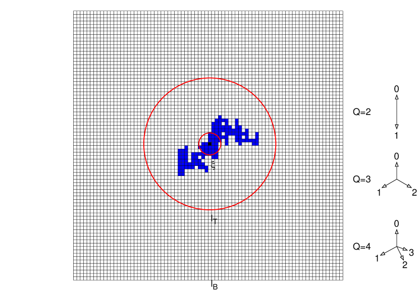
To make the explanation concrete, let us consider $\Lambda_{\rm sq}$ in a temperature-dependent bounding box of $l_{\rm B}\times l_{\rm B}$ (see Fig. ​6). As an initial condition, we take random spin configurations instead of “staggered spin configuration” Evertz2001 because they are neutral and unbiased for all spin states and also prevent a deep penetration of clusters toward the boundary (see below). We fix the seed of the cluster to the origin (the black cell) and perform single cluster updates in order to equilibrate a circular domain. Suppose that $l_{\rm T}$ is its linear dimension. Then, the required number of updates for its equilibration increases exponentially with $l_{\rm T}$ because the off-critical system possesses finite correlation length $\xi$. Roughly speaking, we performed equilibration steps to typically realize $l_{\rm T}\simeq 20\times\xi$ and also use the bounding box with $l_{\rm B}>4\times l_{\rm T}$, where the probability that a cluster touches the bounding box is negligible. Consequently, we can perform measurements of the physical quantity, i.e., correlation functions within the circular domain of $l_{\rm T}$ without finite-size effects Evertz2001 .

Figure 7: Correlation functions $c({\bf r})$ of the $Q$-state Potts model in two directions ($Q=1$ is the bond percolation). For clarity, we draw the lines for MC data points, where the blue (red) ones show $\sqrt{R}c(R)$ in the row (diagonal) direction: ${\bf r}=R{\bf e}_{x}$ [${\bf r}=R({\bf e}_{x}+{\bf e}_{y})/\sqrt{2}$]. With the increase of the temperature $t$, the slopes of lines become steeper, and the discrepancies between blue and red lines become larger.

With respect to the measurement of correlation functions, we can benefit from the so-called improved estimators. In the present case, the correlation function of the Potts model $c({\bf r-r}^{\prime})=\left\langle\sigma_{\bf r}\sigma_{{\bf r}^{\prime}}\right\rangle$ can be calculated as an average over the FK clusters generated by MC, i.e., $c({\bf r-r}^{\prime})=\left\langle(\sigma_{\bf r}\sigma_{{\bf r}^{\prime}})_{\rm impr}\right\rangle_{\rm MC}$, where

$$(\sigma_{\bf r}\sigma_{{\bf r}^{\prime}})_{\rm impr}=\frac{1}{|C_{i}|}\delta({\bf r},{\bf r}^{\prime}|C_{i}).$$ (B3)

The set of sites (the number of sites) in a $i$th cluster were denoted as $C_{i}$ ($|C_{i}|$), and then $\delta({\bf r},{\bf r}^{\prime}|C_{i})=1$ for ${\bf r},{\bf r}^{\prime}\in{C_{i}}$; otherwise, zero.

The correspondence between $q_{\bf r}$ and the magnetic operators is depicted in the right part of Fig. ​6. These magnetic operators can be characterized by the scaling dimensions $x(Q)$, i.e., $x(2)=\frac{1}{8}$, $x(3)=\frac{2}{15}$, $x(4)=\frac{1}{8}$, and also $x(1)=\frac{5}{48}$, which determine the power-law behavior of $c(R)$ at $T_{\rm C}(Q)$ Bloete1982 ; Deng2004 . The fact that Eq. ​(B3) is positive definite is also crucial for calculations of vanishing correlations for large $R/\xi\gg 1$.

For $T>T_{\rm C}(Q)$, we shall provide the raw MC data of the correlation functions in two directions. In Fig. ​7, we exhibit the semilog plots of correlation functions at various temperatures $t=[T-T_{\rm C}(Q)]/T_{\rm C}(Q)$. The pairs of blue and red lines give $\sqrt{R}c(R)$ in the row (${\bf r}=R{\bf e}_{x}$) and the diagonal [${\bf r}=R({\bf e}_{x}+{\bf e}_{y})/\sqrt{2}$] directions. Then, one finds that their slopes become steeper, and the discrepancy of the pair of lines becomes larger with the increase of the reduced temperature $t$. For exactly solved cases, it was revealed that the correlation length is isotropic near critical point, but becomes anisotropic at a distance from it due to the lattice effects. With this in mind, if we suppose the Ornstein-Zernike form of the correlation function as $c(R)\propto{\rm e}^{-R/\xi}/\sqrt{R}$, then our MC data indicate that $\xi$ in the row direction is longer than that in the diagonal direction. Simultaneously, one can notice that the directional dependence of $\xi$ is quite weak, so the extremely accurate data are required to investigate the $Q$ dependence of the ACLs.

Appendix C FITTING CALCULATION OF THE FORM FOR MONTE CARLO DATA

In this Appendix, we detail a fitting procedure of our form (3.2) to the correlation function data provided by the MC simulation calculations. As explained in Appendix ​B, the infinite-size MC method and the improved estimator for the correlation functions has been employed. In typical cases, we performed 1000 independent runs of MC simulations and generated the $10^{11}$ Fortuin-Kasteleyn clusters at each run. Then, for square-lattice sites $i{\bf e}_{x}+j{\bf e}_{y}\in\Lambda_{\rm sq}$ within the equilibrated circular domain $R<l_{\rm T}$ the correlation function data $\{c(i,j)\}$ were obtained, and their statistical errors $\{d(i,j)\}$ were estimated from standard deviations of the averages of the independent runs.

As mentioned in Sec. ​III.1, there exist two sources of errors: the systematic errors stemming from higher bands of eigenvalues which are not taken into account in Eq. ​(3.2) and the statistical errors associated with MC samplings. The former (respectively, latter) becomes larger inward (respectively, outward). We analyze $\{c(i,j)\}$ and $\{d(i,j)\}$ in annular regions ${\cal D}(c_{\rm max},c_{\rm min})$ following the procedure explained below.

We shall take the $Q=3$ and $t=0.15$ case as an example. In Sec. ​III.3, we order-estimated the systematic error as $\Delta(3)\times{\rm e}^{-2R/\bar{\xi}}$ with ${\bar{\xi}}\simeq 2.7$ and $\Delta(3)=1.0-({A}/{\pi})(1-k^{2})^{\frac{1}{4}}\times 2I\simeq O(10^{-2})$. Therefore, to calculate the ACL within a five-digit accuracy, we need to employ an annular region with mean radius $\simeq 20$ or longer. Because the statistical errors are larger in outer regions, we choose ${\cal D}_{0}={\cal D}(1\times 10^{-4},3\times 10^{-5})$ with mean radius $R_{0}\simeq 21.3$ as an optimized region.

Table 3: The ${\cal D}_{\alpha}$ dependence of the estimates of $\xi_{\rm diag}$ and the reduced $\chi^{2}$ values (see text). Other than the optimized region (${\cal D}_{0}$), one inner region (${\cal D}_{-1}$), and two outer regions (${\cal D}_{1}$ and ${\cal D}_{2}$) are defined by $c_{\rm max}$ and $c_{\rm min}$ at each $Q$ and $t$. $R_{\alpha}$ is the mean radius of annular region ${\cal D}_{\alpha}$.

$Q$	$t$	${\cal D}_{\alpha}$	$c_{\rm max}$	$c_{\rm min}$	$|{\cal D}_{\alpha}|$	$R_{\alpha}$	$\xi_{\rm diag}$	$\bar{\chi}^{2}_{|{\cal D}_{\alpha}|}$
1	0.50	${\cal D}_{-1}$	$1\times 10^{-2}$	$1\times 10^{-3}$	432	11.9	2.750670(2)	865
		${\cal D}_{0}$	$1\times 10^{-4}$	$3\times 10^{-5}$	436	22.1	2.750569(1)	0.642
		${\cal D}_{1}$	$1\times 10^{-5}$	$4\times 10^{-6}$	392	27.7	2.750564(4)	0.329
		${\cal D}_{2}$	$5\times 10^{-8}$	$3\times 10^{-8}$	336	41.2	2.75066(7)	1.231
2	0.24	${\cal D}_{-1}$	$1\times 10^{-2}$	$3\times 10^{-3}$	188	10.3	2.734824(1)	0.084
		${\cal D}_{0}$	$1\times 10^{-3}$	$3\times 10^{-4}$	308	16.0	2.734823(4)	0.499
		${\cal D}_{1}$	$3\times 10^{-5}$	$1\times 10^{-5}$	452	24.9	2.734836(8)	0.560
		${\cal D}_{2}$	$1\times 10^{-7}$	$5\times 10^{-8}$	444	39.3	2.7348(1)	0.849
3	0.15	${\cal D}_{-1}$	$1\times 10^{-2}$	$1\times 10^{-3}$	400	11.5	2.672762(3)	240
		${\cal D}_{0}$	$1\times 10^{-4}$	$3\times 10^{-5}$	400	21.3	2.672979(3)	1.10
		${\cal D}_{1}$	$2\times 10^{-6}$	$1\times 10^{-6}$	368	30.6	2.67291(5)	0.810
		${\cal D}_{2}$	$1\times 10^{-7}$	$5\times 10^{-8}$	436	38.3	2.67285(2)	0.496
4	0.10	${\cal D}_{-1}$	$1\times 10^{-2}$	$1\times 10^{-3}$	400	11.5	2.694577	758
		${\cal D}_{0}$	$3\times 10^{-5}$	$1\times 10^{-5}$	428	24.3	2.695252(3)	0.301
		${\cal D}_{1}$	$2\times 10^{-6}$	$1\times 10^{-6}$	348	30.7	2.69525(1)	0.114
		${\cal D}_{2}$	$1\times 10^{-7}$	$5\times 10^{-8}$	452	38.5	2.6951(2)	0.223

Then, we define $\chi^{2}$ as a function of $A,~{}k,~{}b$ by

$$\chi^{2}(A,k,b)=\sum_{(i,j)\in{\cal D}_{0}}\left[\frac{{\cal F}_{\rm sq}(i,j;A,k,b)-c(i,j)}{d(i,j)}\right]^{2},$$ (C1)

We extract values $\bar{A}$, $\bar{k}$, and $\bar{b}$ of the fitting parameters by minimizing $\chi^{2}(A,k,b)$. The first line of the third column in Table ​1 gives their estimates and errors given by the parenthesized digits, which were put based on differences between two results to two groups of independent runs (e.g., we divided 1000 independent runs into two groups and performed fitting calculation for each).

We have expected the extracted values to be obtained under a well-controlled condition of systematic errors by carefully choosing the fitting region. To show concrete evidence to this statement, we perform fittings of data in different annular regions ${\cal D}_{\alpha}$ and check the ${\cal D}_{\alpha}$ dependence of an estimate as well as a reduced $\chi^{2}$ values, i.e.,

$$\bar{\chi}^{2}_{|{\cal D}_{\alpha}|}=\frac{\chi^{2}(\bar{A},\bar{k},\bar{b})}{|{\cal D}_{\alpha}|}.$$ (C2)

The third column of Table ​3 compares the estimates in one inner region (${\cal D}_{-1}$), the optimized region (${\cal D}_{0}$), and two outer regions (${\cal D}_{1}$ and ${\cal D}_{2}$). In general, $\bar{\chi}^{2}_{|{\cal D}_{\alpha}|}$ measures the goodness of fit, which in the present case gives an applicability condition of Eq. ​(3.2) to MC data in ${\cal D}_{\alpha}$. First, one sees that $\bar{\chi}^{2}_{|{\cal D}_{-1}|}$ is much larger than the others, and that $\xi_{\rm diag}$ estimated in ${\cal D}_{-1}$ deviates largely from those in other regions. Meanwhile, the error in $\xi_{\rm diag}$ shown by parenthesized digits becomes smaller for ${\cal D}_{-1}$. These show that Eq. ​(3.2) cannot fit the data in ${\cal D}_{-1}$ due to the systematic errors. Second, one also finds that $\bar{\chi}^{2}_{|{\cal D}_{1}|}$ and $\bar{\chi}^{2}_{|{\cal D}_{2}|}$ are comparable to $\bar{\chi}^{2}_{|{\cal D}_{0}|}$, and that the estimates of $\xi_{\rm diag}$ are almost independent of the choice of the outer regions. Therefore, we conclude that ${\cal D}_{0}$, ${\cal D}_{1}$, and ${\cal D}_{2}$ are in an asymptotic region in which Eq. ​(3.2) can be used for the fitting under the controlled condition of systematic errors, but the statistical errors become larger in outer region.

The first, the second, and the fourth columns of Table ​3 give the results obtained via the same analysis for the $Q=1,\ t=0.50$, the $Q=2,\ t=0.24$, and the $Q=4,\ t=0.10$ cases, respectively. While the overall feature of $Q=1$, 4 is same as that of $Q=3$, the fitting condition for $Q=2$ is clearly different from them, namely, both $\bar{\chi}^{2}_{|{\cal D}_{\alpha}|}$ and $\xi_{\rm diag}$ are almost independent of ${\cal D}_{\alpha}$. This difference can be attributed to the presence/absence of the second band eigenvalue contributions to the correlation function: As explained in Appendix ​A, they are absent in the Ising case so that Eq. ​(3.2) can fit the data in inner annular regions like ${\cal D}_{-1}$.

Table ​1 exhibits the fitting data in optimized regions ${\cal D}_{0}$ for which the convergence check of estimates as demonstrated in Table ​3 has been performed at all temperatures. In principle, we can employ a wider annular region including, e.g., ${\cal D}_{0}$, ${\cal D}_{1}$, and ${\cal D}_{2}$, but, in reality the infinite-size algorithm MC simulations cannot provide reliable averages and meaningful errors for $R\gg\xi_{\rm diag}$ within a moderate computational effort Evertz2001 . Therefore, the optimization of the fitting region is necessary for the purpose of the accurate estimations of the ACLs.

References

- (1) G. Wulff. Xxv. zur frage der geschwindigkeit des wachsthums und der auflösung der krystallflächen. Z. Kristallogr. Cryst. Mater., 34(1):449 – 530, 1901.
- (2) W. K. Burton, N. Cabrera, and F. C. Frank. The growth of crystals and the equilibrium structure of their surfaces. Philos. Trans. R. Soc. London, Ser. A, 243(866):299–358, 1951.
- (3) C. Rottman and M. Wortis. Exact equilibrium crystal shapes at nonzero temperature in two dimensions. Phys. Rev. B, 24:6274–6277, Dec 1981.
- (4) J. E. Avron, H. van Beijeren, L. S. Schulman, and R. K. P. Zia. Roughening transition, surface tension and equilibrium droplet shapes in a two-dimensional ising system. J. Phys. A: Math. Gen., 15(2):L81, 1982.
- (5) R. K. P. Zia and J. E. Avron. Total surface energy and equilibrium shapes: Exact results for the d=2 ising crystal. Phys. Rev. B, 25:2042–2045, Feb 1982.
- (6) Henk van Beijeren. Exactly solvable model for the roughening transition of a crystal surface. Phys. Rev. Lett., 38:993–996, May 1977.
- (7) C. Jayaprakash, W. F. Saam, and S. Teitel. Roughening and facet formation in crystals. Phys. Rev. Lett., 50:2017–2020, Jun 1983.
- (8) M. Fujimoto. Equilibrium crystal shape of the potts model at the first-order transition point. J. Phys. A: Math. Gen., 30(11):3779, 1997.
- (9) M. Fujimoto. Eight-vertex model: Anisotropic interfacial tension and equilibrium crystal shape. J. Stat. Phys., 67(1):123–154, Apr 1992.
- (10) M. Fujimoto. Equilibrium crystal shape of hard squares with diagonal attractions. J. Phys. A: Math. Gen., 26(10):2285, 1993.
- (11) R. J. Baxter. Exactly Solved Models in Statistical Mechanics. Academic Press, London, 1982.
- (12) F. Y. Wu. The potts model. Rev. Mod. Phys., 54:235–268, Jan 1982.
- (13) H. N. V. Temperley, Elliott H Lieb, and Samuel Frederick Edwards. Relations between the percolation and colouring problem and other graph-theoretical problems associated with regular planar lattices: some exact results for the percolation problem. Proceedings of the Royal Society of London. A. Mathematical and Physical Sciences, 322(1549):251–280, 1971.
- (14) R. J. Baxter. Potts model at the critical temperature. J. Phys. C: Solid State Phys., 6(23):L445, 1973.
- (15) A. Klümper, A. Schadschneider, and J. Zittartz. Inversion relations, phase transitions and transfer matrix excitations for special spin models in two dimensions. Z. Phys. B, 76(2):247–258, Jun 1989.
- (16) E. Buffenoir and S. Wallon. The correlation length of the potts model at the first-order transition point. J. Phys. A: Math. Gen., 26(13):3045–3062, jul 1993.
- (17) Christian Borgs and Wolfhard Janke. An explicit formula for the interface tension of the 2d potts model. J. Phys. I France, 2(11):2011–2018, 1992.
- (18) R. K. P. Zia. Duality of interfacial energies and correlation functions. Physics Letters A, 64(4):345 – 347, 1978.
- (19) L. Laanait. Discontinuity of surface tensions in the q-state potts model. Physics Letters A, 124(9):480 – 484, 1987.
- (20) M. Holzer. Equilibrium crystal shapes and correlation lengths: A general exact result in two dimensions. Phys. Rev. Lett., 64:653–656, Feb 1990.
- (21) Y. Akutsu and N. Akutsu. Interface tension, equilibrium crystal shape, and imaginary zeros of partition function: Planar ising systems. Phys. Rev. Lett., 64:1189–1192, Mar 1990.
- (22) S. B. Rutkevich. Comment on ’equilibrium crystal shape of the potts model at the first-order transition point’. J. Phys. A: Math. Gen., 35(34):7549, 2002.
- (23) M. Fujimoto. Reply to ’comment on ”equilibrium crystal shape of the potts model at the first-order transition point”’. J. Phys. A: Math. Gen., 35(34):7553, 2002.
- (24) M. Fujimoto. Anisotropic correlation length in the eight-vertex model. Physica A, 233(1):485 – 502, 1996.
- (25) M. Holzer. Exact equilibrium crystal shapes in two dimensions for free-fermion models. Phys. Rev. B, 42:10570–10582, Dec 1990.
- (26) H. G. Vaidya. The spin-spin correlation functions and susceptibility amplitudes for the two-dimensional ising model; triangular lattice. Physics Letters A, 57(1):1 – 4, 1976.
- (27) R. K. P. Zia. Exact equilibrium shapes of ising crystals on triangular/honeycomb lattices. J. Stat. Phys., 45(5):801–813, Dec 1986.
- (28) M. Fujimoto. Duality relations and equilibrium crystal shapes of potts models on triangular and honeycomb lattices. Physica A, 264(1):149 – 170, 1999.
- (29) M. Fujimoto. Auxiliary vertices method for kagomé-lattice eight-vertex model. J. Stat. Phys., 90(1):363–388, Jan 1998.
- (30) M. Fujimoto. Anisotropic interfacial tension and the equilibrium crystal shape of kagomé-lattice eight-vertex model. J. Phys. A: Math. Gen., 35(7):1517, 2002.
- (31) Morton Hamermesh. Group Theory and Its Application to Physical Problems. Dover, New York, 1989.
- (32) C. M. Fortuin and P. W. Kasteleyn. On the random cluster model. 1. introduction and relation to other models. Physica, 57:536–564, 1972.
- (33) J. D. Johnson, S. Krinsky, and B. M. McCoy. Vertical-arrow correlation length in the eight-vertex model and the low-lying excitations of the -- hamiltonian. Phys. Rev. A, 8:2526–2547, Nov 1973.
- (34) J. D. Johnson, S. Krinsky, and B. M. McCoy. Critical index of the vertical-arrow correlation length in the eight-vertex model. Phys. Rev. Lett., 29:492–494, Aug 1972.
- (35) M. Fujimoto. Hard-hexagon model: Anisotropy of correlation length and interfacial tension. J. Stat. Phys., 59(5):1355–1381, Jun 1990.
- (36) M. Fujimoto. Hard-hexagon model: Calculation of anisotropic interfacial tension from asymptotic degeneracy of largest eigenvalues of row-row transfer matrix. J. Stat. Phys., 61(5-6):1295–1304, 1990.
- (37) A. Klümper. Investigation of excitation spectra of exactly solvable models using inversion relations. Int. J. Mod. Phys. B, 04(05):871–893, 1990.
- (38) Rodney Baxter. Asymptotically degenerate maximum eigenvalues of the eight-vertex model transfer matrix and interfacial tension. J. Stat. Phys., 8(1):25–55, 1973.
- (39) L. P. Kadanoff. Spin-spin correlations in the two-dimensional ising model. Il Nuovo Cimento B (1965-1970), 44(2):276–305, Aug 1966.
- (40) H. Cheng and T. T. Wu. Theory of toeplitz determinants and the spin correlations of the two-dimensional ising model. iii. Phys. Rev., 164:719–735, Dec 1967.
- (41) B. M. McCoy and T. T. Wu. The Two-Dimensional Ising Model. Harvard University Press, Cambridge, Massachusetts, 1973.
- (42) Keiji Yamada. On the Spin-Spin Correlation Function in the Ising Square Lattice. Prog. Theor. Phys., 69(4):1295–1298, 04 1983.
- (43) K. Yamada. On the Spin-Spin Correlation Function in the Ising Square Lattice and the Zero Field Susceptibility. Prog. Theor. Phys., 71(6):1416–1418, 06 1984.
- (44) Keiji Yamada. Pair Correlation Function in the Ising Square Lattice: —Generalized Wronskian Form—. Prog. Theor. Phys., 76(3):602–612, 09 1986.
- (45) T. T. Wu, B. M. McCoy, C. A. Tracy, and E. Barouch. Spin-spin correlation functions for the two-dimensional ising model: Exact theory in the scaling region. Phys. Rev. B, 13:316–374, Jan 1976.
- (46) William J. Camp and Michael E. Fisher. Behavior of two-point correlation functions at high temperatures. Phys. Rev. Lett., 26:73–77, Jan 1971.
- (47) Michael E. Fisher and William J. Camp. Behavior of two-point correlation functions near and on a phase boundary. Phys. Rev. Lett., 26:565–568, Mar 1971.
- (48) R. Z. Bariev and M. P. Zhelifonov. Spin-spin correlation function of the plane ising lattice. Theor. Math. Phys., 25(1):1012–1018, 1975.
- (49) M. Fujimoto. Spatial anisotropy and rotational invariance of critical hard squares. J. Phys. A: Math. Gen., 27(15):5101, 1994.
- (50) M. Namba. Geometry of Projective Algebraic Curves. Monographs and textbooks in pure and applied mathematics. M. Dekker, New York, 1984.
- (51) Walter Selke and Julia M Yeomans. A monte carlo study of the asymmetric clock or chiral potts model in two dimensions. Zeitschrift für Physik B Condensed Matter, 46(4):311–318, 1982.
- (52) P. Peczak and D. P. Landau. Monte carlo study of finite-size effects at a weakly first-order phase transition. Phys. Rev. B, 39:11932–11942, Jun 1989.
- (53) Sourendu Gupta and A. Irbäck. Physics beyond instantons. measuring the physical correlation length. Physics Letters B, 286(1):112 – 117, 1992.
- (54) W. Janke and S. Kappler. Correlation length of 2d potts models: numerical vs exact results. Nucl. Phys. B, Proc. Suppl., 34:674 – 676, 1994.
- (55) W. Janke and S. Kappler. Monte carlo study of cluster-diameter distribution: An observable to estimate correlation lengths. Phys. Rev. E, 56:1414–1420, Aug 1997.
- (56) Y. Akutsu and N. Akutsu. Novel numerical method for studying the equilibrium crystal shape. J. Phys. Soc. Jpn., 56(1):9–12, 1987.
- (57) N. Akutsu and Y. Akutsu. Equilibrium crystal shape:two dimensions and three dimensions. J. Phys. Soc. Jpn., 56(7):2248–2251, 1987.
- (58) Walter Selke. Droplets in two-dimensional ising and potts models. J. Stat. Phys., 56(5-6):609–620, 1989.
- (59) H. G. Evertz and W. von der Linden. Simulations on infinite-size lattices. Phys. Rev. Lett., 86:5164–5167, May 2001.
- (60) A. Hintermann, H. Kunz, and F. Y. Wu. Exact results for the potts model in two dimensions. J. Stat. Phys., 19(6):623–632, Dec 1978.
- (61) M. P. M. den Nijs. A relation between the temperature exponents of the eight-vertex and q-state potts model. J. Phys. A: Math. Gen., 12(10):1857–1868, oct 1979.
- (62) M. P. Nightingale and H. W. J. Blöte. Finite size scaling and critical point exponents of the potts model. Physica A: Statistical Mechanics and its Applications, 104(1):352 – 357, 1980.
- (63) H. W. J. Blöte and M. P. Nightingale. Critical behaviour of the two-dimensional potts model with a continuous number of states; a finite size scaling analysis. Physica A: Statistical Mechanics and its Applications, 112(3):405 – 465, 1982.
- (64) A. Aharony and D. Stauffer. Introduction to Percolation Theory. Taylor & Francis, London, 2003.
- (65) Y. Higuchi. SUGAKU (in Japanese), 40(3):247–254, 1988.
- (66) M. Aizenman and D. J. Barsky. Sharpness of the phase transition in percolation models. Commun. Math. Phys., 108(3):489–526, Sep 1987.
- (67) M. V. Menshikov. Coincidence of critical points in percolation problems. Soviet Math. Dokl., 33:856–859, 1986.
- (68) C. Jayaprakash and W. F. Saam. Thermal evolution of crystal shapes: The fcc crystal. Phys. Rev. B, 30:3916–3928, Oct 1984.
- (69) Mark Holzer and Michael Wortis. Low-temperature expansions for the step free energy and facet shape of the simple-cubic ising model. Phys. Rev. B, 40:11044–11058, Dec 1989.
- (70) M. Suzuki. New universality of critical exponents. Prog. Theor. Phys., 51(6):1992–1993, 1974.
- (71) Y. Chan, A. J. Guttmann, B. G. Nickel, and J. H. H. Perk. The ising susceptibility scaling function. J. Stat. Phys., 145(3):549–590, Nov 2011. and the references therein.
- (72) R. J. Baxter. Solvable eight-vertex model on an arbitrary planar lattice. Philos. Trans. R. Soc. Lond., Ser. A, 289(1359):315–346, 1978.
- (73) R. H. Swendsen and Jian-Sheng Wang. Nonuniversal critical dynamics in monte carlo simulations. Phys. Rev. Lett., 58:86–88, Jan 1987.
- (74) U. Wolff. Lattice field theory as a percolation process. Phys. Rev. Lett., 60:1461–1463, Apr 1988.
- (75) U. Wolff. Collective monte carlo updating for spin systems. Phys. Rev. Lett., 62:361–364, Jan 1989.
- (76) Y. Deng, H. W. J. Blöte, and B. Nienhuis. Backbone exponents of the two-dimensional q-state potts model: A monte carlo investigation. Phys. Rev. E, 69:026114, Feb 2004.