Galaxy simulation with the evolution of grain size distribution

Abstract

We compute the evolution of interstellar dust in a hydrodynamic simulation of an isolated disc galaxy. We newly implement the evolution of full grain size distribution by sampling 32 grid points on the axis of the grain radius. We solve it consistently with the chemical enrichment and hydrodynamic evolution of the galaxy. This enables us to theoretically investigate spatially resolved evolution of grain size distribution in a galaxy. The grain size distribution evolves from a large-grain-dominated ($\gtrsim 0.1~{}\micron$) phase to a small-grain production phase, eventually converging to a power-law-like grain size distribution similar to the so-called MRN distribution. We find that the small-grain abundance is higher in the dense ISM in the early epoch ($t\lesssim 1$ Gyr) because of efficient dust growth by accretion, while coagulation makes the small-grain abundance less enhanced in the dense ISM later. This leads to steeper extinction curves in the dense ISM than in the diffuse ISM in the early phase, while they show the opposite trend later. The radial trend of extinction curves is described by faster evolution in the inner part. We also confirm that the simulation reproduces the observed relation between dust-to-gas ratio and metallicity, and the radial gradients of dust-to-gas ratio and dust-to-metal ratio in nearby galaxies. Since the above change in the grain size distribution occurs in $t\sim 1$ Gyr, the age and density dependence of grain size distribution has a significant impact on the extinction curves even at high redshift.

1 Introduction

Dust grains contained in the interstellar medium (ISM) evolve together with galaxies. Dust plays an important role at various stages of galaxy evolution in the following aspects. Molecular hydrogen, which is the main constituent of molecular clouds, forms on dust surfaces. Thus, dust enrichment induces an environment rich in molecular clouds that eventually host star formation (Hirashita & Ferrara, 2002; Cazaux & Tielens, 2004; Yamasawa et al., 2011). In addition, dust also acts as a coolant in the late stages of star formation, inducing the fragmentation of gas clouds (Omukai et al., 2005) . This determines the typical mass of stars (Schneider et al., 2006) and the shape stellar initial mass function (IMF) (e.g. Casuso & Beckman, 2012). All the above processes occur on grain surfaces. The total grain surface area is governed not only by the grain abundance but also by the distribution function of grain size (grain size distribution); therefore, the evolution of these two aspects of dust grains is fundamentally important for the thorough understanding of galaxy evolution.

Dust is also important in radiative processes. Dust grains absorb ultraviolet (UV)–optical stellar light and reemit infrared (IR) photons. Thus, the spectral energy distribution (SED) is dramatically changed by dust grains (e.g. Takeuchi et al., 2005). This means that a part of star formation activities in galaxies are obscured by dust. This obscured fraction is only recovered by the observations of IR dust emission; thus, tracing the dust emission is crucial in estimating the total star formation rate (SFR) (e.g. Buat & Xu, 1996; Inoue et al., 2000; Kennicutt & Evans, 2012). Because the absorption efficiency of UV photons depends strongly on the grain size distribution through the extinction curve as well as on the total dust abundance (e.g. Calzetti, 2001), the two aspects of dust (namely, the total dust abundance and the grain size distribution) are important in understanding galaxy evolution.

A comprehensive model that computes the evolution of grain size distribution has been developed by Asano et al. (2013b), who took into account all major processes that drive the change of grain size distribution in a one-zone model of a galaxy. Dust condenses from the metals ejected from supernovae (SNe) (e.g. Kozasa et al., 1989; Todini & Ferrara, 2001; Nozawa et al., 2003; Bianchi & Schneider, 2007; Nozawa et al., 2007) and asymptotic giant branch (AGB) stars (e.g. Ferrarotti & Gail, 2006; Ventura et al., 2014; Dell’Agli et al., 2017). This dust production by stellar sources is the starting point of dust evolution. Calculations of dust condensation and processing in stellar ejecta indicate that grains are biased to large sizes ($a\gtrsim 0.1~{}\micron$, where $a$ is the grain radius) (Nozawa et al., 2007; Yasuda & Kozasa, 2012; Dell’Agli et al., 2017). Subsequently, dust grains are processed in the ISM as described by Asano et al. (2013b) and Hirashita & Aoyama (2019, hereafter HA19). The interstellar processing starts with shattering, which gradually converts large grains into small ones. As the system is enriched with metals, the accretion of gas-phase metals onto dust grains becomes efficient in the dense ISM. This causes a drastic increase of the grain abundance at $a\lesssim 0.03~{}\micron$ because small grains have larger surface-to-volume ratios (recall that the accretion rate is proportional to the grain surface area). Accretion is saturated when a significant fraction of gas-phase metals are used up; and subsequently, coagulation converts small grains into large grains, smoothing the grain size distribution towards a power-law shape similar to the Mathis et al. (1977, hereafter MRN) grain size distribution.

In reality, the evolution of dust is strongly affected by the ambient physical condition such as gas metallicity, temperature, and density. Although Asano et al. (2013b) succeeded in calculating the evolution of grain size distribution, their one-zone model is not capable of treating the spatial variation of dust evolution that depends on the ISM conditions. The evolution of ISM is governed by hydrodynamical processes. Thus, hydrodynamic simulations have been used to study the evolution of ISM in galaxies (e.g. Wada & Norman, 2007; Saitoh et al., 2008; Marinacci et al., 2014; Kim et al., 2014, 2016; Marinacci et al., 2019; Li et al., 2019; Graziani et al., 2019). For the purpose of considering the effects of ISM evolution on dust properties, it would be ideal to treat dust evolution in a manner consistent with the hydrodynamical development of the ISM. However, it is in general computationally expensive to implement the evolution of grain size distribution in already heavy hydrodynamic simulations.

In the past, most hydrodynamic simulations with dust evolution calculated only the total dust abundance without grain size distribution. Dayal et al. (2010) post-processed a cosmological hydrodynamic simulation with a dust evolution model which includes stellar dust production and SN destruction, and calculated the expected submillimetre fluxes for high-redshift star-forming galaxies. Yajima et al. (2015), using a cosmological zoom-in simulation, calculated the dust distribution in high-redshift galaxies by simply assuming a constant dust-to-metal ratio. Bekki (2015) treated dust as a new particle species in addition to the gas, dark matter and star particles in their hydrodynamic simulations. In order to calculate the evolution of dust in galaxies, they included not only the formation and destruction of dust, but also the effect of dust on star formation and stellar feedback. McKinnon et al. (2016) performed cosmological zoom-in simulations by modelling dust as a component coupled with the gas. They included the processes relevant for the formation and evolution of dust, and revealed the importance of dust growth by the accretion of gas-phase metals. In addition, McKinnon et al. (2017) ran cosmological simulations to calculate the statistical properties of dust in galaxies. They broadly reproduced the dust abundances in the present-day galaxies, although they tended to underestimate those in high-redshift dusty galaxies. Zhukovska et al. (2016) analysed the dust evolution in an isolated Milky-Way-like galaxy by post-processing a hydrodynamic simulation. They put particular focus on the effect of gas-temperature-dependent sticking coefficient on dust growth by accretion, in order to reproduce the relation between silicon depletion and gas density. Hu et al. (2019) simulated the dust evolution in the ISM, focusing on dust destruction by sputtering. Although they did not trace the entire galaxy, their focus on a small region in the ISM enabled them to resolve the structures associated with SN shocks. We also note that there are some non-hydrodynamic approaches using semi-analytic models that predicted the evolution of dust mass in galaxies (Popping et al., 2017; de Bennassuti et al., 2014; Ginolfi et al., 2018; Vijayan et al., 2019).

Aoyama et al. (2017, hereafter A17) implemented a two-size grain model in the cosmological smoothed particle hydrodynamics (SPH) code gadget3-osaka (A17; Shimizu et al. 2019), which is a modified version of gadget-3 (originally described in Springel, 2005, as gadget-2). Their treatment of dust is based on the two-size approximation (Hirashita, 2015), in which the entire grain radius range is divided into ‘large’ and ‘small’ grains. The two-size approximation reduces the computational cost in calculating the evolution of grain size distribution, so that it is easily implemented in hydrodynamic simulations. A17 performed simulations of a Milky-Way-like isolated galaxy, and explained the radial distribution of the total dust abundance of nearby galaxies in Mattsson & Andersen (2012). A17 also predicted a variation of grain size distribution along the galactic radius. Hou et al. (2017) took advantage of the grain size information in A17 and investigated the temporal and spatial variation of extinction curves. They also examined the dependence of extinction curves on metallicity. They found that extinction curves become steeper at the intermediate age and metallicity when the dust abundance is strongly modified by the accretion of gas-phase metals, and at low densities where shattering is more efficient than coagulation. Using the same simulation, Chen et al. (2018) calculated the abundance of H₂ and CO in a consistent manner with the dust abundance and grain size distribution, which govern the grain-surface reaction rates and UV shielding. They found that H₂ is not a good tracer of SFR at low metallicity because H₂-rich regions are limited to dense compact regions.

The above framework with the two-size approximation has also been applied to cosmological simulations (Aoyama et al., 2018; Gjergo et al., 2018; Aoyama et al., 2019; Hou et al., 2019). For example, Aoyama et al. (2018) explained the observed relation between dust-to-gas ratio and metallicity, the evolution of the comoving dust mass density in the Universe, and the radial profile of dust surface density around massive galaxies. Hou et al. (2019), using the same simulation setup but including a simple treatment for active galactic nucleus feedback, focused on the relations between dust-related quantities and galaxy characteristics. They broadly reproduced the statistical properties such as the dust mass function and the relation between dust-to-gas ratio and metallicity in the nearby Universe. They also investigated extinction curves. However, because these results are based on the two-size approximation, the accuracy of extinction curve is limited. There is another approach for the evolution of grain size distribution based on the method of moments formulated by Mattsson (2016). This method is powerful in calculating the processes related to the moments of grain size distribution such as the total grain surface area. However, it is still difficult to calculate the extinction curves. An explicit solution for the full grain size distribution enables us to directly calculate the extinction curves as well as other quantities (e.g. the surface area) that require grain size information.

Recently, there have been some efforts to directly solve the evolution of full grain size distribution in galaxy-scale hydrodynamic simulations. McKinnon et al. (2018) developed a computational code that solves the evolution of full grain size distribution in an adaptive mesh hydrodynamic simulation code, AREPO (Springel, 2010). They showed some test calculations of an isolated galaxy, but realistic calculations to be compared with observations need further implementation of, for example, stellar feedback. Hirashita & Aoyama (2019, hereafter HA19) took another approach to solve the evolution of full grain size distribution. They post-processed an isolated-galaxy simulation: they chose some SPH gas particles and derived the evolution of grain size distribution on each particle based on its history of physical conditions (mainly gas density, temperature, and metallicity). They successfully derived the grain size distribution similar to the MRN distribution at ages comparable to the Milky Way ($\gtrsim 3$ Gyr). However, because their calculation was based on post-processing, the results may depend on the frequency of snapshots; that is, we cannot capture the change of physical conditions shorter than the output snapshot interval ($10^{7}$ yr in the above post-processing). Indeed, the processes occurring in dense environments such as coagulation and accretion could have a shorter characteristic time-scales in metal-rich regions (A17). To obtain robust results against such potentially quick processes, we need to solve the evolution of grain size distribution and that of hydrodynamical structures simultaneously.

The goal of this paper is to implement the evolution of full grain size distribution directly in a hydrodynamic simulation to obtain a self-consistent view of grain size distribution with ISM evolution. We use an isolated-galaxy simulation, which could achieve a higher spatial resolution of the ISM compared with cosmological simulations. Two improvements with respect to previous studies are expected: one is direct knowledge of full grain size distribution without relying on the two-size approximation. This leads to a better understanding of the quantities for which the grain size distribution is essential (such as extinction curves). The other is a better capability of treating the dust growth processes (accretion and coagulation), which could occur quickly. Such quick processes cannot be captured robustly by post-processing so that a simultaneous calculation of grain size distribution and hydrodynamics is essential.

This paper is organized as follows. In Section 2, we introduce the calculation method for the grain size distribution and the scheme of the simulation. In Section 3, we show the results and comparison with observations. In Section 4, we provide additional discussions. Section 5 concludes this paper. Throughout this paper, we adopt the solar metallicity $Z_{\sun}=0.02$ for the convenience of direct comparison with our previous simulations. We also use the terms ‘small’ and ‘large’ grain radius to roughly indicate the grain radius smaller and larger than $\sim 0.03~{}\micron$.

2 Model

2.1 Hydrodynamic simulation

We perform a hydrodynamic simulation of an isolated galaxy using the smoothed particle hydrodynamics (SPH) code gadget3-osaka (A17; Shimizu et al., 2019), which is based on the gadget-3 code (originally described in Springel, 2005). In our simulation, the star formation and metal/dust production are treated consistently with gravitational/hydrodynamic evolution of a Milky-Way-like isolated galaxy. Dust grains are assumed to be coupled with gas particles (Section 2.2).

Our present run corresponds to the M12 run in Shimizu et al. (2019), and the total mass of isolated galaxy is $\sim 10^{12}~{}{\rm M}_{\sun}$. We employ $10^{5}$ dark matter particles, $10^{5}$ gas (SPH) particles, $10^{5}$ and $1.25\times 10^{4}$ collisionless particles that represent stars in the disc and the bulge, respectively. We adopt a fixed gravitational softening length of $\epsilon_{\rm grav}=80$ pc, but allow the minimum gas smoothing length to reach 10 percent of $\epsilon_{\rm grav}$. The final gas smoothing length reaches $\sim 30$ pc as the gas becomes denser owing to radiative cooling.

The difference between this paper and A17 is as follows. We additionally include the metal/dust supply and the feedback from AGB stars. We use the CELib package (Saitoh, 2017) for metal generation and follow 13 chemical abundances (H, He, C, N, O, Ne, Mg, Si, S, Ca, Fe, Ni, and Eu). The ejection of metals and energy from stars are treated separately for SNe Ia, II, and AGB stars as a function of time after the onset of star formation. The delay-time distribution function of SN Ia rate is modeled with a power-law of $t^{-1}$ (Totani et al., 2008; Maoz & Mannucci, 2012). In comparison, in A17, the metal and dust were injected instantaneously after 4 Myr from the onset of star formation, whose masses were simply proportional to the stellar mass. For more details of the stellar feedback with CELib in our simulations, we refer the interested reader to Shimizu et al. (2019). We further describe the dust enrichment by stellar sources in the next subsection.

2.2 Evolution of grain size distribution

We use the same model as in HA19 for the evolution of grain size distribution. The model is based on Asano et al. (2013b), but with simplifications that do not lose the physical essence of the relevant processes. These simplifications are useful for the implementation in hydrodynamic simulations. For the dust evolution processes, we consider stellar dust production, dust destruction by SN shocks in the ISM, dust growth by accretion and coagulation in the dense ISM, and dust disruption by shattering in the diffuse ISM. We assume that the dust grains are dynamically coupled with the gas, which is usually valid on the spatial scales of interest in this paper (McKinnon et al., 2018). In what follows, we only describe the outline of the model to be implemented for individual SPH gas particles (hereafter, referred to simply as gas particles). We refer the interested reader to HA19 for the complete set of equations and the details.

The grain size distribution at time $t$ is expressed by the grain mass distribution $\rho_{\mathrm{d}}(m,\,t)$, which is defined such that $\rho_{\mathrm{d}}(m,\,t)\,\mathrm{d}m$ ($m$ is the grain mass and $t$ is the time) is the mass density of dust grains whose mass is between $m$ and $m+\mathrm{d}m$. We assume grains to be spherical and compact, so that $m=(4\pi/3)a^{3}s$, where $a$ is the grain radius and $s$ is the material density of dust. We adopt $s=3.5$ g cm^-3 based on silicate in Weingartner & Draine (2001). The grain mass distribution is related to the grain size distribution, $n(a,\,t)$, as

$$\rho_{\mathrm{d}}(m,\,t)\,\mathrm{d}m=\frac{4}{3}\pi a^{3}sn(a)\,\mathrm{d}a.$$ (1)

The total dust mass density $\rho_{\mathrm{d,tot}}(t)$ is

$$\rho_{\mathrm{d,tot}}(t)=\int_{0}^{\infty}\rho_{\mathrm{d}}(m,\,t)\,\mathrm{d}m.$$ (2)

The gas density, $\rho_{\rm gas}$, is given by the number density of hydrogen nuclei, $n_{\mathrm{H}}$ as $\rho_{\mathrm{gas}}=\mu m_{\mathrm{H}}n_{\mathrm{H}}$ ($\mu=1.4$ is the gas mass per hydrogen, and $m_{\mathrm{H}}$ is the mass of hydrogen atom). The dust-to-gas ratio, $\mathcal{D}(t)$, is defined as

$$\mathcal{D}_{\mathrm{tot}}(t)\equiv\frac{\rho_{\mathrm{d,tot}}(t)}{\rho_{\mathrm{gas}}(t)}.$$ (3)

Note that the evolution of $\rho_{\mathrm{gas}}$ is calculated by the hydrodynamic simulation for each gas particle.

The time-evolution of $\rho_{\mathrm{d}}(m,\,t)$ is described by

$$\frac{\partial\rho_{\mathrm{d}}(m,\,t)}{\partial t} =\left[\frac{\partial\rho_{\mathrm{d}}(m,\,t)}{\partial t}\right]_{\mathrm{star}}+\left[\frac{\partial\rho_{\mathrm{d}}(m,\,t)}{\partial t}\right]_{\mathrm{sput}}$$

$$+\left[\frac{\partial\rho_{\mathrm{d}}(m,\,t)}{\partial t}\right]_{\mathrm{acc}}+\left[\frac{\partial\rho_{\mathrm{d}}(m,\,t)}{\partial t}\right]_{\mathrm{shat}}$$

$$+\left[\frac{\partial\rho_{\mathrm{d}}(m,\,t)}{\partial t}\right]_{\mathrm{coag}}+\rho_{\mathrm{d}}(m,\,t)\frac{\mathrm{d}\ln\rho_{\mathrm{gas}}}{\mathrm{d}t},$$ (4)

where the terms with subscripts ‘star’, ‘sput’, ‘acc’, ‘shat’ and ‘coag’ indicate the changing rates of grain mass distribution by stellar dust production, sputtering, accretion, shattering, and coagulation, respectively, and the last term is caused by the change of background gas density. Below we briefly describe each term. We actually solve discrete forms and adopt 32 grid points for the discrete grain size distribution in the range of $3\times 10^{-4}-10\,\micron$.

2.2.1 Stellar dust production

We estimate the increase of dust mass by stellar dust production, assuming a constant dust condensation efficiency, $f_{\mathrm{in}}=0.1$, of the ejected metals (Inoue, 2011; Kuo et al., 2013). Using the metal production rate per volume, $\dot{\rho}_{\rm Z}$, calculated in the simulations, we write the change of the grain size distribution by stellar dust production as

$$\left[\frac{\partial\rho_{\mathrm{d}}(m,\,t)}{\partial t}\right]_{\mathrm{star}}=f_{\mathrm{in}}\dot{\rho}_{Z}\,m\tilde{\varphi}(m),$$ (5)

where $m\tilde{\varphi}(m)$ is the mass distribution function of the dust grains produced by stars, and it is normalized so that the integration for the whole grain mass range is unity. The grain size distribution of the dust grains produced by stars [which is related to the above mass distribution as $\varphi(a)\,\mathrm{d}a\equiv\tilde{\varphi}(m)\,\mathrm{d}m$] is written as

$${\varphi}(a)=\frac{C_{\varphi}}{a}\exp\left\{-\frac{[\ln(a/a_{0})]^{2}}{2\sigma^{2}}\right\},$$ (6)

where $C_{\varphi}$ is the normalization factor, $\sigma$ is the standard deviation, and $a_{0}$ is the central grain radius. We adopt $\sigma=0.47$ and $a_{0}=0.1\,\micron$ following Asano et al. (2013b).

2.2.2 Dust destruction and growth

As shown by HA19, dust destruction by sputtering in SN shocks and dust growth by accretion are both described by the following same form of equation:

$$\left[\frac{\partial\rho_{\mathrm{d}}(m,\,t)}{\partial t}\right]_{\mathrm{sput/acc}}=-\frac{\partial}{\partial m}[\dot{m}\rho_{\mathrm{d}}(m,\,t)]+\frac{\dot{m}}{m}\rho_{\mathrm{d}}(m,\,t).$$ (7)

where $\dot{m}\equiv\mathrm{d}m/\mathrm{d}t$. We estimate that

$$\dot{m}=\xi(t)m/\tau_{\mathrm{dest/acc}}(m),$$ (8)

where $\tau_{\mathrm{dest/acc}}(m)$ is the grain-mass-dependent time-scale of destruction or accretion. In the actual computations, we solve the effects of destruction and accretion, separately. For destruction, we formally choose $\xi(t)=-1$. For accretion, $\xi(t)$ is the fraction of metals in the gas-phase [i.e. the fraction $(1-\xi)$ is condensed into the dust phase]. Therefore,

$$\xi(t)\equiv\begin{cases}1-\mathcal{D}_{\rm tot}/Z\,\,&{(\rm accretion)},\\ -1\,\,&{(\rm destruction)},\end{cases}$$ (9)

where $Z$ is the metallicity.

The destruction time-scale $\tau_{\mathrm{dest}}(m)$ is estimated based on the sweeping time-scale divided by the grain-mass-dependent destruction efficiency as (e.g. McKee, 1989)

$$\tau_{\mathrm{dest}}(m)=\frac{M_{\mathrm{gas}}}{\epsilon_{\mathrm{dest}}(m)M_{\mathrm{s}}\gamma},$$ (10)

where $M_{\mathrm{gas}}$ is the mass of the gas particle of interest, $M_{\mathrm{s}}=6800$ M_☉ is the gas mass swept by a single SN blast, $\gamma$ is the rate of SNe sweeping the gas, $\epsilon_{\rm dest}(m)$ is the dust destruction efficiency as a function of grain mass. We adopt the following empirical expression for the destruction efficiency (described as a function of $a$ instead of $m$):

$$\epsilon_{\rm dest}(a)=1-\exp\left[-0.1\left(\frac{a}{0.1\,\micron}\right)^{-1}\right].$$ (11)

For accretion, the growth time-scale is estimated as (we fixed the sticking efficiency $S=0.3$ in HA19)

$$\tau_{\mathrm{acc}}(m) =\frac{1}{3}\tau^{\prime}_{\mathrm{0,acc}}\left(\frac{a}{0.1~{}\micron}\right)\left(\frac{Z}{\mathrm{Z}_{\sun}}\right)^{-1}\left(\frac{n_{\mathrm{H}}}{10^{3}\,\mathrm{cm}^{-3}}\right)^{-1}\left(\frac{T_{\mathrm{gas}}}{10\,\mathrm{K}}\right)^{-1/2},$$ (12)

where $\tau^{\prime}_{\mathrm{0,acc}}$ is a constant (we adopt $\tau^{\prime}_{\mathrm{0,acc}}=1.61\times 10^{8}$ yr appropriate for silicate, but the value for graphite has little difference; Hirashita, 2012), and $T_{\mathrm{gas}}$ is the gas temperature.

2.2.3 Shattering and coagulation

Shattering and coagulation are described by grain–grain collisions followed by the redistribution of fragments or coagulated grains (Jones et al., 1994; Jones et al., 1996; Hirashita & Yan, 2009). Shattering is assumed to occur only in the diffuse medium ($n_{\mathrm{H}}<1$ cm^-3) where the grain velocities are high enough. For coagulation, since we cannot spatially resolve the dense and cold medium where it occurs, we adopt a sub-grid model. We assume that coagulation occurs in gas particles which satisfy $n_{\mathrm{H}}>10$ cm^-3 and $T_{\mathrm{gas}}<1000$ K, and that a mass fraction of $f_{\mathrm{dense}}=0.5$ of such a dense particle is condensed into dense clouds, hosting coagulation, with $n_{\mathrm{H}}=10^{3}$ cm^-3 and $T_{\mathrm{gas}}=50$ K on subgrid scales.

The time evolution of grain size distribution by shattering or coagulation is expressed as

$$\left[\frac{\partial\rho_{\mathrm{d}}(m,\,t)}{\partial t}\right]_{\mathrm{shat/coag}}=-m\rho_{\mathrm{d}}(m,\,t)\int_{0}^{\infty}\alpha(m_{1},\,m)\rho_{\mathrm{d}}(m_{1},\,t)\mathrm{d}m_{1}$$

$$+\int_{0}^{\infty}\int_{0}^{\infty}\alpha(m_{1},\,m_{2})\rho_{\mathrm{d}}(m_{1},\,t)\rho_{\mathrm{d}}(m_{2},\,t)\mu_{\mathrm{shat/coag}}(m;\,m_{1},\,m_{2})\mathrm{d}m_{1}\mathrm{d}m_{2},$$ (13)

where $\mu_{\mathrm{shat/coag}}$ describes the grain mass distribution function of newly formed shattered fragments or coagulated grains, and $\alpha$ is expressed in collisions between grains with masses $m_{1}$ and $m_{2}$ (radii $a_{1}$ and $a_{2}$, respectively) as

$$\alpha(m_{1},\,m_{2})\equiv\frac{\sigma_{1,2}v_{1,2}}{m_{1}m_{2}},$$ (14)

where $\sigma_{1,2}=\pi(a_{1}+a_{2})^{2}$ and $v_{1,2}$ are the collisional cross-section and the relative velocity between the two grains (we explain how to evaluate $v_{1,2}$ later).

We adopt the following formula for the grain velocity in a turbulent medium:

$$v_{\mathrm{gr}}(a) =1.1\mathcal{M}^{3/2}\left(\frac{a}{0.1~{}\micron}\right)^{1/2}\left(\frac{T_{\mathrm{gas}}}{10^{4}~{}\mathrm{K}}\right)^{1/4}\left(\frac{n_{\mathrm{H}}}{1~{}\mathrm{cm}^{-3}}\right)^{-1/4}$$

$$\times\left(\frac{s}{3.5~{}\mathrm{g~{}cm}^{-3}}\right)^{1/2}~{}\mathrm{km~{}s}^{-1},$$ (15)

where $\mathcal{M}$ is the Mach number of the largest-eddy velocity. We adopt $\mathcal{M}=3$ for shattering and $\mathcal{M}=1$ for coagulation to effectively achieve the grain velocity levels suggested by Yan et al. (2004). In considering the collision rate between two grains with $v_{\mathrm{gr}}=v_{1}$ and $v_{2}$, we estimate the relative velocity $v_{1,2}$ by $v_{1,2}=(v_{1}^{2}+v_{2}^{2}-2v_{1}v_{2}\mu_{1,2})^{1/2}$, where $\mu=\cos\theta$ ($\theta$ is an angle between the two grain velocities) is randomly chosen between $-1$ and 1 in every calculation of $\alpha$. The above expression for the velocity (with $\mathcal{M}=1$) was originally derived by Ormel et al. (2009) who assumed the maximum eddy size to be the Jeans length and the maximum velocity dispersion to be the sound velocity. We simply use their functional form for the purpose of avoiding grain velocity calculations in every time-step, but modify it to scale the maximum velocity (with the Mach number) to match with the velocity scale adopted for our previously adopted models based on Yan et al. (2004). As shown by Hirashita & Kobayashi (2013), detailed dependence of grain velocities on the grain radius is not essential, but the overall velocity level is more important. In particular, it is essential that large ($a\gtrsim 0.1~{}\micron$) grains attain velocities higher than a few km s^-1 in the diffuse ISM, since shattering, which plays an important role in the first production of small grains, does not occur otherwise. We will surely need to combine our simulation with direct dust motion calculations (e.g. Hopkins & Lee, 2016; McKinnon et al., 2018) to check if the velocity levels assumed here are actually achieved. Because of the huge computational cost required, we leave this for a future work.

For shattering, the total mass of the fragments is estimated following Kobayashi & Tanaka (2010). We consider a collision of two dust grains with masses $m_{1}$ and $m_{2}$. The total mass of the fragments ejected from $m_{1}$ is estimated as

$$m_{\mathrm{ej}}=\frac{\phi}{1+\phi}m_{1},$$ (16)

where $\phi\equiv{E_{\mathrm{imp}}}/(m_{1}Q_{\mathrm{D}}^{\star})$ [$E_{\mathrm{imp}}=\frac{1}{2}{m_{1}m_{2}}v_{\mathrm{1,2}}^{2}/(m_{1}+m_{2})$ is the impact energy and $Q_{\mathrm{D}}^{\star}$ is the specific impact energy that causes the catastrophic disruption (i.e. the disrupted mass is $m_{1}/2$)]. We adopt $Q_{\mathrm{D}}^{\star}=4.3\times 10^{10}$ cm² s^-2 (valid for silicate). Now we set the grain size distribution of shattered fragments. The maximum and minimum grain masses of the fragments are assumed to be $m_{\mathrm{f,max}}=0.02m_{\mathrm{ej}}$ and $m_{\mathrm{f,min}}=10^{-6}m_{\mathrm{f,max}}$, respectively (Guillet et al., 2011). We adopt the following fragment mass distribution including the remnant of mass $m_{1}-m_{\mathrm{ej}}$ as

$$\mu_{\mathrm{shat}}(m,\,m_{1},\,m_{2}) =\frac{(4-\alpha_{\mathrm{f}})m_{\mathrm{ej}}m^{(-\alpha_{\mathrm{f}}+1)/3}}{3\left[m_{\mathrm{f,max}}^{\frac{4-\alpha_{\mathrm{f}}}{3}}-m_{\mathrm{f,min}}^{\frac{4-\alpha_{\mathrm{f}}}{3}}\right]}\,\Phi(m;\,m_{\mathrm{f,min}},\,m_{\mathrm{f,mmax}})$$

$$+(m_{1}-m_{\mathrm{ej}})\delta(m-m_{1}+m_{\mathrm{ej}}),$$ (17)

where $\Phi(m;\,m_{\mathrm{f,min}},\,m_{\mathrm{f,mmax}})=1$ if $m_{\mathrm{f,min}}<m<m_{\mathrm{f,mmax}}$, and 0 otherwise, $\delta$ is Dirac’s delta function, and $\alpha_{\rm f}$ is the power-law index of the fragment size distribution ($\alpha_{\rm f}=3.3$; Jones et al. 1996). Grains whose radii are smaller than the minimum grain radius ($3\times 10^{-4}~{}\micron$) are removed.

For coagulation, we adopt

$$\mu_{\mathrm{coag}}=m_{1}\delta(m-m_{1}-m_{2})$$ (18)

in equation (13).

2.3 Calculation of extinction curves

Extinction curves describe the wavelength dependence of the optical depth of dust. Extinction curves have been useful in constraining the grain size distribution (e.g. Weingartner & Draine, 2001). Here, we calculate extinction curves based on the grain size distributions, $n_{i}(a)$, where $i$ indicates the composition of the dust grains (we consider multiple compositions as we explain below). The extinction at wavelength $\lambda$ in units of magnitude is written as

$$A_{\lambda}=(2.5\log_{10}\mathrm{e})L\displaystyle\sum_{i}\displaystyle\int_{0}^{\infty}n_{i}(a)\,\pi a^{2}Q_{\rm ext}(a,\lambda),$$ (19)

where $L$ is the path length, $Q_{\rm ext}(a,\lambda)$ is the extinction efficiency factor, which is evaluated by using the Mie theory (Bohren & Huffman, 1983) with the same optical constants for silicate and carbonaceous dust (graphite) as in Weingartner & Draine (2001). In this paper, the mass fractions of silicate and carbonaceous dust are fixed to 0.54 and 0.46, respectively (number ratio 0.43:0.57) with both grain species having the same grain size distribution (Hirashita & Yan, 2009). Because this fraction is valid only for the Milky Way, we concentrate on the comparison with the Milky Way extinction curve below. For more comprehensive comparison, we need a more sophisticated model of the evolution of grain compositions (Hou et al., 2016), which is left for a future work. To concentrate on the extinction curve shape, the extinction is normalized to the value in the $V$ band ($\lambda^{-1}=1.8\,\mu{\rm m}^{-1}$); that is, we output $A_{\lambda}/A_{V}$ (so that $L$ is cancelled out).

3 Results

3.1 Evolution of grain size distribution

3.1.1 Dense and diffuse ISM

We show the general features in the evolution of grain size distribution. This also serves as a test against the post-processing results in HA19. We choose the gas particles contained in $0<R<7\,{\rm kpc}$ and $|z|<0.3\,{\rm kpc}$, where we adopt a cylindrical coordinate with $R$ and $z$ being the radial and vertical coordinates, respectively ($z=0$ is the disc plane). In order to investigate the dependence on the local physical condition, we divide the gas particles into two categories: the dense (cold) and diffuse (warm) gas. The dense (cold) gas particles are chosen by $T_{\mathrm{gas}}<10^{3}$ K and $n_{\mathrm{H}}>10\,{\rm cm}^{-3}$, while the diffuse (warm) ones by $0.1<n_{\mathrm{H}}<1$ cm^-3 and $10^{3}<T_{\mathrm{gas}}<10^{4}$ K. These criteria are the same as those adopted by HA19, but HA19 defined these by the physical condition at $t=10$ Gyr. We use the physical condition at each snapshot so that our definition in this paper really traces the current dense and diffuse phases. We choose the ages $t=0.3$, 1, and 3 Gyr. These ages are basically chosen for comparison with A17. Although A17 also examined $t=10$ Gyr snapshot, the snapshot at $t=3$ Gyr represents the dust evolution at the oldest stage with a metallicity comparable to the present Milky Way; thus, discussions in this paper do not change even if we choose $t>3$ Gyr instead of $t=3$ Gyr.

In Fig. 1, we show the grain size distributions at each age for the dense and diffuse gas particles separately with the median and 25th and 75th percentiles at each grain radius bin. The dust is dominated by the large grains at young ages ($t\lesssim 0.3$ Gyr) because stellar dust production is the major source of dust. Since star formation tends to be associated with dense regions in the galaxy, the peak in the grain size distribution is higher in the dense medium than in the diffuse medium. This leads to more efficient small-grain production by shattering in the dense gas particles because of higher rates of grain–grain collisions. In the dense ISM, the small grains produced by shattering are further processed by accretion, which forms a bump (second peak) at $a\sim 0.01~{}\micron$. The bump is formed at smaller radii than the main peak because the large surface-to-volume ratios of small grains lead to efficient accretion (Kuo & Hirashita, 2012).

As shown in the middle panel of Fig. 1 at $t=1$ Gyr, the grain abundance becomes larger at all grain radii than at $t=0.3$ Gyr, because of further dust enrichment. The increase at small grain radii is more significant than that at large radii because of further dust processing by shattering and accretion. In particular, dust and metal abundances are large enough for efficient accretion at this stage. Therefore, the bump created by accretion around $a\sim 0.01~{}\micron$ is commonly observed in the grain size distributions. The dense gas particles have more large grains than the diffuse ones for two reasons: one is the same as above (we find more dense gas particles in actively star-forming regions), and the other is more efficient coagulation in the dense ISM. Indeed, we observe that coagulation depletes the smallest grains in the dense ISM.

In the bottom panel of Fig. 1, we show that at $t=3$ Gyr, the evolutionary trend seen at $t=1$ Gyr is more pronounced. Coagulation further proceeds especially in the dense medium, producing a smooth power-law-like grain size distribution similar to the MRN grain size distribution [$n(a)\propto a^{-3.5}$]. The effect of dust growth by accretion is also imprinted in the grain size distribution in the diffuse ISM as seen in the bump around $a\sim 0.01~{}\micron$. This imprinted bump is caused when these particles were previously included in the dense ISM, where accretion could take place efficiently if the metallicity is high enough. Because of the variety in the past history, the diffuse gas particles have larger variation in the grain size distribution especially at small grain radii than the dense ones. In some regions as shown in the lower 25th percentile, there is no bump at small grain radii, indicating that accretion has not yet been efficient. Thus, we predict that there is a large variety in the dust abundance in the diffuse ISM.

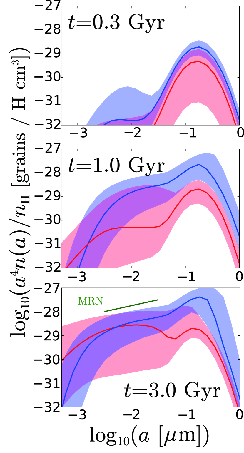
Figure 1: Evolution of grain size distribution for the entire galactic disc at $t=0.3$, 1, and 3 Gyr from top to bottom. The blue and red lines show the median grain size distribution in the dense and diffuse gas particles, respectively. The shaded regions show the areas between 25th and 75th percentiles. For the vertical axis, we present the grain size distribution per hydrogen (H) multiplied by $a^{4}$: the resulting quantity is proportional to the grain mass distribution per $\log_{10}a$. The linear (green) solid line marked with ‘MRN’ in the bottom panel shows the power-law slope of the MRN grain size distribution [$n(a)\propto a^{-3.5}$].

3.1.2 Radial dependence

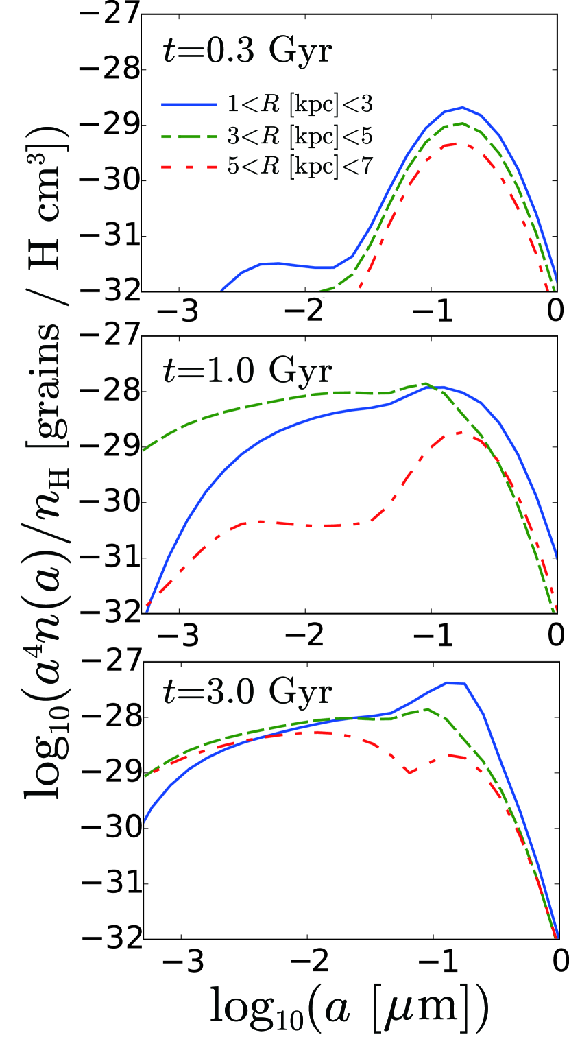
Figure 2: Grain size distribution at three different galactic radius ranges for the snapshots at $t=0.3,1.0,$ and 3.0 Gyr from top to bottom. The blue (solid), green (dashed) and red (dot-dashed) lines correspond to the radial ranges of $R=1$–3, 3–5, and 5–7 kpc, respectively. In order to avoid the overlap of the shades, only median lines are displayed, but the dispersions are similar to those shown in Fig. 1.

We analyze the spatial variation of grain size distribution. In order to concentrate on the dust in the galactic disc, we select the gas particles in $|z|<0.3\,{\rm kpc}$. In Fig. 2, we show the radial dependence of the grain size distribution in each snapshot by presenting the median at $R=1$–3, 3–5, and 5–7 kpc. To make the presentation simple, we only plot the median, but we expect similar dispersions to those shown in Fig. 1. At $t=0.3$ Gyr, the grain size distributions in all regions are similar, dominated by large grains produced by stars. The dust abundance is the highest in the centre, which is due to more active star formation and resulting metal enrichment at smaller galactic radii. Small-grain production by shattering is slightly seen only in the inner region, but interstellar processing is not efficient at all radii.

As shown in the middle panel of Fig. 2, at $t=1.0$ Gyr, the grain size distributions are significantly modified by interstellar processing. At the outer radii ($R=5$–7 kpc), the grain abundance is still dominated by large grains. At the intermediate radii ($R=3$–5 kpc), accretion enhances the abundance of small grains because accretion time-scale of smaller grains is shorter than that of large ones (Section 3.1.1). The increased small grains also shatters large grains, causing a sharp drop of grain size distribution at $a\gtrsim 0.3~{}\micron$. At the inner radii ($R=1$–3 kpc), in addition to the two processes above, coagulation is also efficient because the grain abundance and gas density are the highest among the three $R$ ranges. The effect of coagulation is clear in the depletion of the smallest grains and the enhancement of the large grain abundance at $a\gtrsim 0.1~{}\micron$. We note that the grain size distribution does not change monotonically along the galactic radius: the strongest enhancement of small grains relative to large grains is seen at intermediate radii.

The bottom panel of Fig. 2 shows the grain size distributions at $t=3$ Gyr. At this age, the small-grain abundance is enhanced to a similar level at all radii. In this phase, the initially observed log-normal shape is erased by interstellar processing. The inner region has a higher large-grain abundance because of more efficient coagulation. Since the inner region also hosts more efficient accretion, the dust abundance is the highest.

3.2 Evolution of dust abundance

3.2.1 Dust-to-gas ratio and metallicity

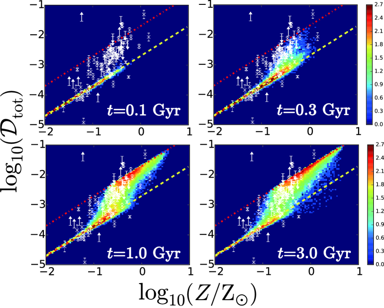
Figure 3: Distribution of gas particles on the $\mathcal{D}_{\rm tot}$–$Z$ plane at $t=0.1,0.3,1$ and 3 Gyr as labeled. The colour indicates the logarithmic surface density of the gas particle on this diagram as shown in the colour bars. The yellow dashed and red dot-dashed lines present the linear relations of the stellar yield $(\mathcal{D}_{\rm tot}=f_{\rm in}Z)$ and the saturation limit $(\mathcal{D}_{\rm tot}=Z)$, respectively. For comparison, we also show the observational data in Rémy-Ruyer et al. (2014) and Zhukovska (2014) (white points with error bars or upper/lower limits).

We examine whether the evolution of the total dust abundance is reasonably calculated by our model. The relation between dust-to-gas ratio ($\mathcal{D}_{\mathrm{tot}}$; equation 3) and metallicity ($Z$) is often used to test if the dust evolution is correctly treated in a chemical evolution framework (e.g. Lisenfeld & Ferrara, 1998). We plot the relation between $\mathcal{D}_{\mathrm{tot}}$ and $Z$ for all gas particles in Fig. 3. We also show a simple constant dust-to-metal ratios expected from pure stellar dust production, $\mathcal{D}_{\rm tot}=f_{\rm in}Z$ (yellow dashed line), and the saturation limit, $\mathcal{D}_{\rm tot}=Z$ (red dot-dashed line).

We observe in Fig. 3 that a fixed dust-to-metal ratio is a good approximation in the early phase ($t\la 0.1$ Gyr), since the dust evolution is driven by stellar sources. Dust growth by accretion, whose efficiency (or time-scale) has a metallicity dependence (equation 12), causes a nonlinear increase of $\mathcal{D}_{\mathrm{tot}}$ at $Z\gtrsim 0.1$ Z_☉ as seen after $t=0.3$ Gyr. Because of this nonlinearity, the dust-to-metal ratio is not constant (see also Dwek, 1998; Hirashita, 1999a, b; Inoue, 2003; Zhukovska et al., 2008; Asano et al., 2013a). For example, Inoue (2003) argued that the $\mathcal{D}_{\rm tot}$ increases rapidly by accretion when the galactic age is $\sim 0.3$ Gyr. Our simulation results are consistent with their results. As the system is enriched with metals, the $\mathcal{D}_{\rm tot}$–$Z$ relation extends towards higher metallicities and higher $\mathcal{D}_{\rm tot}$. Because dust growth by accretion is limited by the available gas-phase metals (Section 2.2.2), the increase of $\mathcal{D}_{\rm tot}$ as a function of $Z$ becomes moderate at the highest metallicities. Naturally, $\mathcal{D}_{\mathrm{tot}}$ does not exceed $Z$ (i.e. the simulation data are always located below the line of $\mathcal{D}_{\mathrm{tot}}=Z$).

We also plot the observed $\mathcal{D}_{\rm tot}$–$Z$ relation for nearby galaxies with each point corresponding to individual galaxy (not spatially resolved) (Rémy-Ruyer et al., 2014; Zhukovska, 2014). Note that our plots show each gas particle within a single galaxy. Thus, we use their observational data only as a first reference to judge if our dust evolution model correctly reproduces the observationally expected relation. Our model roughly reproduces the observation, indicating that our implementation of various dust formation and processing mechanisms is successful in catching the trend of dust evolution as a function of metallicity.

A17 also performed a similar hydrodynamic simulation of an isolated galaxy with dust enrichment but using a simplified model for the grain size distribution (two-size approximation). The $\mathcal{D}_{\rm tot}$–$Z$ relation in A17 (see their Fig. 7) is similar to that obtained in this paper. Indeed, at $t\lesssim 0.3$ Gyr, the $\mathcal{D}_{\rm tot}$–$Z$ relation follows the one expected from the stellar dust production ($\mathcal{D}_{\rm tot}=f_{\rm in}Z$). At $t\gtrsim 1$ Gyr, the non-linearity in the $\mathcal{D}_{\rm tot}$–$Z$ relation appears owing to dust growth by accretion, asymptotically approaching to $\mathcal{D}_{\rm tot}=Z$. However, there are some differences between our results and A17’s. A17 showed a larger dispersion in the $\mathcal{D}_{\rm tot}$–$Z$ relation even at $Z<0.1$ Z_☉. Since the increase of dust-to-gas ratio in this regime is driven by accretion (dust growth), A17 shows a clear dust mass increase by accretion at $Z<0.1$ Z_☉, while our current simulation indicates that occurs accretion at $Z>0.1$ Z_☉. In other words, A17 has more efficient accretion. Indeed, A17’s fig. 8 shows that the increase of small grains happens at $Z<0.1$ Z_☉ at $t=0.3$ Gyr, while our current simulation does not show any enhancement of small-grain abundance at $t=0.3$ Gyr (Fig. 1). In the two-size approximation, all small grains are assumed to have a single radius of $5\times 10^{-3}~{}\micron$, while in our case shattering supplies a continuous spectrum of grain radii. Therefore, the accretion rate increases drastically once small grains are produced in the two-size approximation, while accretion is enhanced more gradually in our simulation. The difference indicates that there is a risk of overestimating dust growth by accretion at low metallicity in the two-size approximation.

3.2.2 Radial dependence

In Fig. 4, we compare the radial dependence of the dust-to-gas mass ratio [here we express it as a function of $R$, $\mathcal{D}_{\rm tot}(R)$]. We adopt a mass-weight average for the dust-to-gas ratio as

$$\mathcal{D}_{\rm tot}(R)\equiv\dfrac{\displaystyle\sum_{R-\Delta R/2<R_{i}<R+\Delta R/2}m^{\rm gas}_{i}\mathcal{D}^{\rm tot}_{i}}{\displaystyle\sum_{R-\Delta R/2<R_{i}<R+\Delta R/2}m^{\mathrm{gas}}_{i}},$$ (20)

where $R_{i}$ and $m^{\mathrm{gas}}_{i}$ are the radial coordinate and the mass of the $i$th gas particle, respectively, and the summation is taken for all the gas particles in each radial bin of width $\Delta R$. Here we choose gas particles in the disc ($|z|<0.3$ kpc). We use 40 bins on the linear scale in $0\leq R\leq 10$ kpc.

We adopt the same observational data as in A17. The data are compiled by Mattsson & Andersen (2012), who originally adopted the sample from Muñoz-Mateos et al. (2009) (chosen from the Spitzer Infrared Nearby Galaxies Survey sample; Kennicutt et al. 2003). We adopt these data because of the completeness and uniformity of the quantities that are directly compared with the outputs of our simulation, with a note that there are some new data of spatially resolved dust emission (De Vis et al., 2019; Chiang et al., 2018). Mattsson & Andersen (2012) investigated the radial profile of dust-to-gas ratio and dust-to-metal ratio in nearby star-forming galaxies (mainly spirals). They used the metallicity calibration method of Moustakas et al. (2010). We categorize the observational sample by typical ages using the specific star formation rate (sSFR), following the same criterion as in A17. We choose four ranges: sSFR $>10\,{\rm Gyr}^{-1}$, $1\,{\rm Gyr}^{-1}<{\rm sSFR}<10\,{\rm Gyr}^{-1}$ and sSFR $<1\,{\rm Gyr}^{-1}$, which are referred to as Category I, II, and III, respectively. They are compared with the snapshots at $t=0.3,1$, and 3 Gyr. To cancel the galaxy size effect, we normalise the radius by $R_{25}$ (the radius at which surface brightness falls to 25 mag arcsec^-2) for the observational sample, following Mattsson & Andersen (2012). We also evaluate $R_{25}$ for the simulated galaxies by using the relation $R_{25}\simeq 4R_{\rm d}$, where $R_{\rm d}$ is the scale length of stellar disk (Elmegreen, 1998). In order to obtain $R_{\rm d}$, we performed fitting for the stellar surface density profile of simulated galaxy at each epoch. The value of $R_{25}$ changes as time passes, because the distribution of stellar component changes: $R_{25}=6.9$, 7.0, and 7.2 kpc at $t=0.3$, 1, and 3 Gyr, respectively.

We plot the radial profile of $\mathcal{D}_{\rm tot}$ of each category in Fig. 4. The dust-to-gas ratio in the ‘youngest’ phase represented by Category I (Holmberg II) is broadly reproduced in terms of not only the slope but also the absolute value (Fig. 4a). In this phase, since the dust enrichment is dominated by stellar dust production, the dust-to-gas ratio is proportional to the metallicity; thus, the variation of $\mathcal{D}_{\mathrm{tot}}$ along the galactic radius directly traces the metallicity gradient.

In Fig. 4b, we compare the galaxies in Category II with the simulation result at $t=1$ Gyr. We observe that the level and slope of the radial profile are both reproduced well. Compared with the result at $t=0.3$ Gyr, the dust-to-gas ratios are larger at all galactic radii, and the slope is steeper. In the central part, accretion has drastically increased the dust abundance, while stellar dust production is still dominant at the outer radii. Therefore, the contrast of dust-to-gas ratio between the central and outer parts is the largest in this epoch. Accordingly, the radial slope of $\mathcal{D}_{\mathrm{tot}}$ is the steepest.

We further compare the galaxies in Category III with the simulation result at $t=3$ Gyr in Fig. 4c. Although the observed data points have a large dispersion, the simulation overall reproduces both the value and slope of $\mathcal{D}_{\mathrm{tot}}$. In other words, the simulation result lies in the middle of the observational data. Compared with the radial distribution at $t=1$ Gyr, the dust-to-gas ratio is larger at all radii, especially in the outer part, because dust growth by accretion has been prevalent also there. The slope is shallower at $t=3$ Gyr than at 1 Gyr.

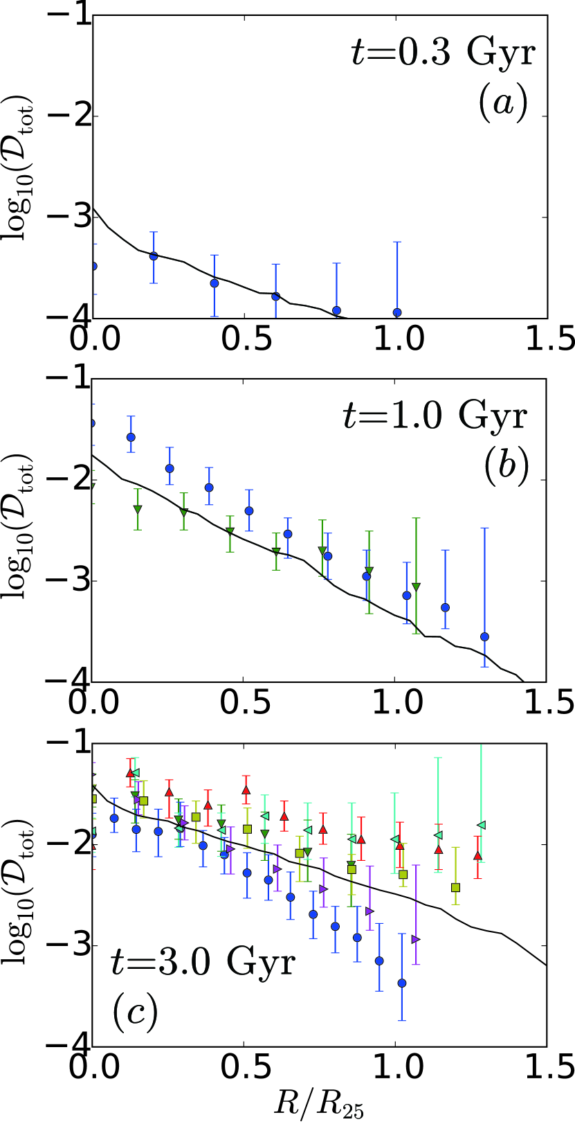
Figure 4: Comparison of the radial profiles of dust-to-gas ratio at $t=0.3$, 1, and 3 Gyr [panels (a), (b), and (c), respectively] with the observational data compiled by Mattsson & Andersen (2012). The solid line is the radial profile of dust-to-gas ratio for each snapshot of the simulation. We scaled the radius with $R_{25}$ (see text). In panel (a), the filled circles with error bars represent the observational radial profile of Holmberg II. In panel (b), the circle and triangle points show NGC 3621 and NGC 925, respectively. In panel (c), the circle, $\bigtriangledown$, $\bigtriangleup$, $\lhd$, $\rhd$, and square symbols correspond to NGC 2403, NGC 4736, NGC5055, NGC 5194, NGC628 and NGC 7793, respectively.

The dust-to-metal ratio traces the fraction of metals condensed into the solid phase. Different processes affect the dust-to-metal ratio differently. Indeed, Mattsson et al. (2012) showed by analytic arguments that the radial profile of dust-to-metal ratio could be used to identify the dominant dust enrichment process. The dust-to-metal ratio in each radial bin is estimated by dividing the mass-weighted dust-to-gas ratio by the mass-weighted metallicity as

$$\dfrac{\mathcal{D}_{\rm tot}}{Z}(R)=\dfrac{\displaystyle\sum_{R-\Delta R/2<R_{i}<R+\Delta R/2}m^{\rm gas}_{i}D_{{\rm tot},i}}{\displaystyle\sum_{R-\Delta R/2<R_{i}<R+\Delta R/2}m^{\rm gas}_{i}Z^{\rm gas}_{i}}\,,$$ (21)

where the summation is taken in each radial bin in the same way as in equation (20) with a constraint of $|z|<0.3$ kpc.

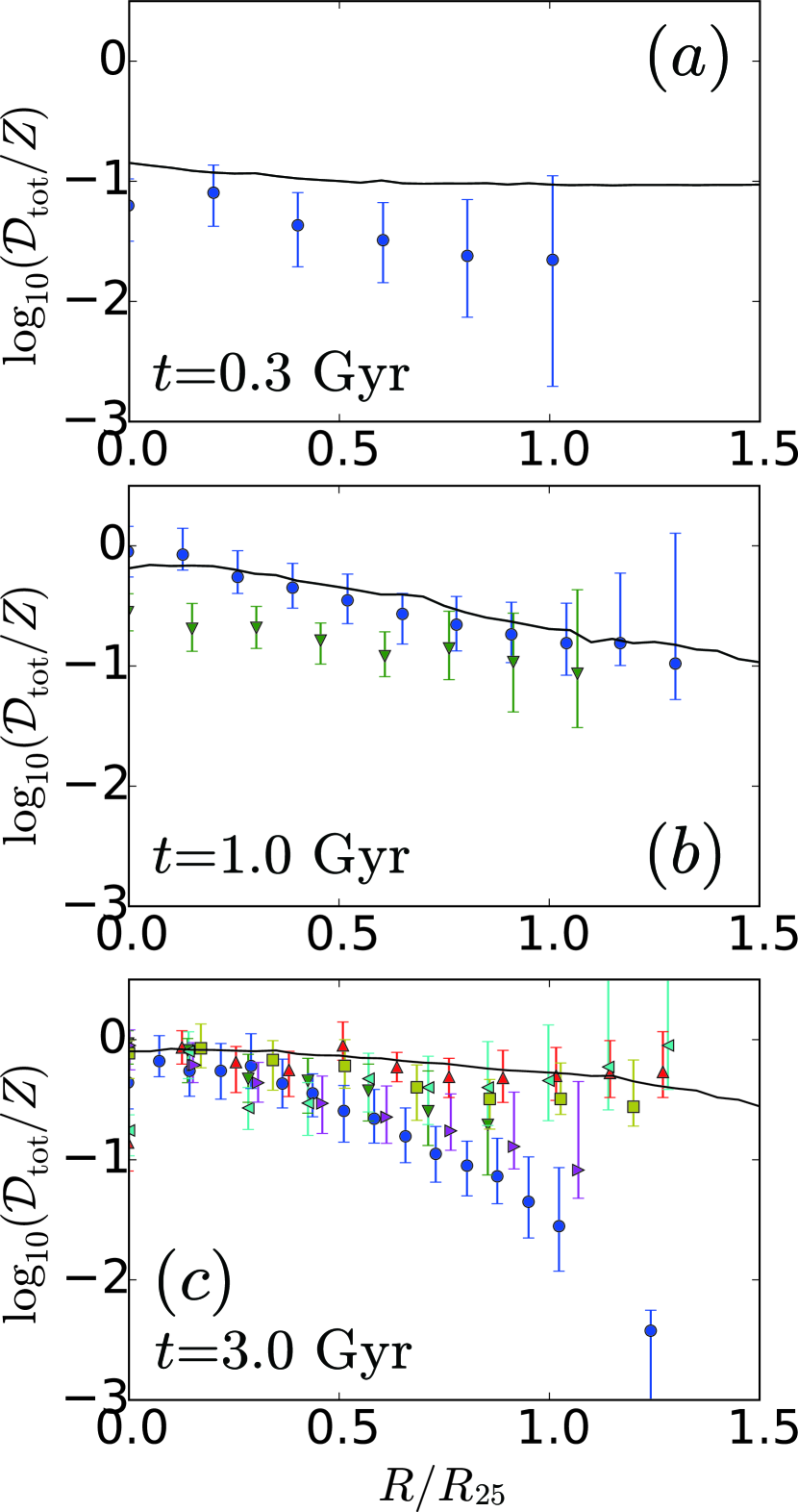
Figure 5: Same as Fig. 4 but presenting the radial profile of dust-to-metal ratio.

In Fig. 5, we find that the dust-to-metal ratio is almost constant in the early phase at $t=0.3$ Gyr and that the flat trend is broadly consistent with the data of Holmberg II (Category I) considering the large errors. At this stage, the level of dust-to-metal ratio is broadly determined by the condensation efficiency in stellar ejecta. Thus, the dust-to-metal ratio is almost constant ($\simeq f_{\rm in}=0.1$), and its radial profile is flat.

For the galaxies in Category II, which we compare with the simulation at $t=1$ Gyr in Fig. 5b, we find that the profile of dust-to-metal ratio is broadly consistent with the observational data, considering the large error bars. The decreasing trend of dust-to-metal ratio with increasing radius is caused by more efficient accretion in the centre than in the outer regions, since accretion favours metal-rich environments (see also Mattsson et al., 2012; Mattsson & Andersen, 2012). Accordingly, the slope of the dust-to-metal ratio profile is the steepest around this epoch. We emphasize that, since the dust-to-metal ratio is not constant, we should at least take non-constant dust-to-metal ratios (both temporally and spatially) into account in modeling the dust evolution in galaxies.

The galaxies in Category III are compared with the snapshot at $t=3$ Gyr in Fig. 5c. The simulation somewhat overproduces the dust-to-metal ratios at large radii, although some galaxies are consistent with our result even at the outer radii. The radial gradient of dust-to-metal ratio is shallower at $t=3$ Gyr than at $t=1$ Gyr, because the effect of accretion becomes more prevalent up to larger radii at later times. NGC 2403 shows a steep decline of dust-to-metal ratio at the outer radii, which cannot be explained by our models.

The radial profiles of dust-to-gas ratio and dust-to-metal ratio are similar to the previous simulation that used the two-size approximation (A17). This means that the two-size approximation adopted in A17 is good enough if we only calculate the total dust abundance. We point out that the tendency of overestimating the dust-to-metal ratio at $t=3$ Gyr (Fig. 5c) is also observed in A17. This could be due to an overestimate of dust growth by accretion. We discuss this issue in Section 4.

3.3 Extinction curves

3.3.1 Dependence on the ISM phases

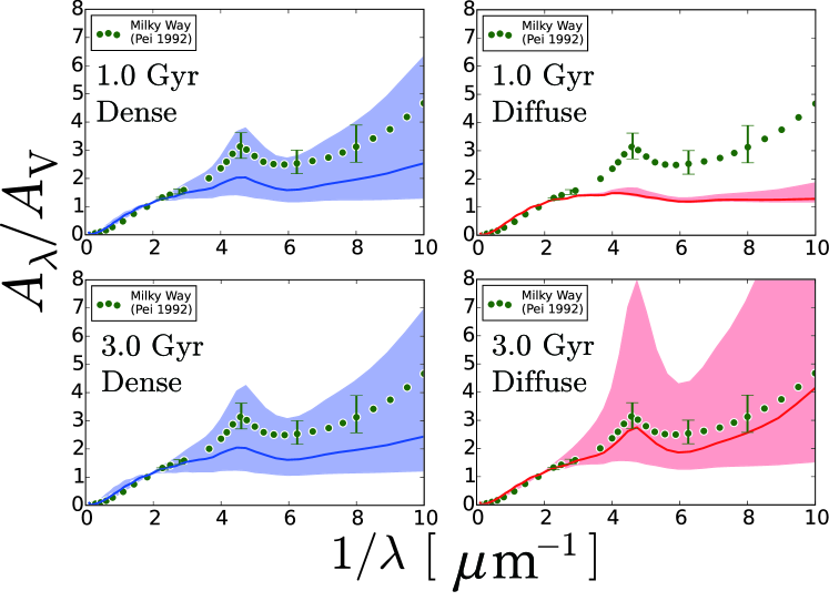
Figure 6: Variation of extinction curves at $t=1$ and 3 Gyr for the dense and diffuse gas particles as indicated in each panel. The solid line is the median and the shaded region shows the area between the 25 and 75 percentiles. We also show the observed Milky Way extinction curve (Pei, 1992) by the green circles. The error bars show the dispersion for various lines of sight taken from Fitzpatrick & Massa (2007) (see also Nozawa & Fukugita, 2013).

As representative observable dust properties that reflect the grain size distribution, we calculate the extinction curves by the method described in Section 2.3. In Fig. 6, we show the extinction curves for the dense and diffuse gas particles. We sorted the extinction curves ($A_{\lambda}/A_{\rm V}$) and obtained the median and 25th and 75th percentile for each of the dense and diffuse particles. We only show the extinction curves at $t=1$ and 3 Gyr. At $t<1$ Gyr, the extinction curves are similar to the ones in the diffuse gas at $t=1$ Gyr, because they are determined by the log-normal grain size distribution of stellar dust. Thus, we only focus on $t\geq 1$ Gyr. At $t=1$ Gyr, the extinction curves in the diffuse medium are flat as mentioned above. In the dense regions, in contrast, the extinction curves have more variety, reflecting more efficient small grain production as shown in Fig. 1. As explained in Section 3.1.1, the dust-to-gas ratio in the dense gas particles tends to be higher since the dense regions are more metal-enriched. Thus, shattering and accretion affect the grain size distributions more in the dense medium than in the diffuse medium. Consequently, steeper extinction curves appear in the dense ISM at $t=1$ Gyr.

At $t=3$ Gyr, the extinction curve shape has a large variety at UV wavelengths, especially in the diffuse ISM. As we observe in Fig. 1, the variety in the grain size distribution is large at grain radii $a\lesssim 0.03\,\micron$ at $t=3$ Gyr, which affects the extinction at $\lambda\sim 2\pi a\sim 0.2~{}\micron$. Since the diffuse gas particles have a larger variety in the grain size distribution around $a\sim 0.03\,\micron$ than the dense ones, the variety in the extinction curves is greater in the diffuse ISM. The median extinction curve is slightly steeper in the diffuse ISM at $t=3$ Gyr, contrary to the results at $t=1$ Gyr.

In Fig. 6, we also plot the observed Milky Way extinction curve as a reference. The observational data is taken from Pei (1992) and the dispersion adopted from Fitzpatrick & Massa (2007) and Nozawa & Fukugita (2013) is also shown at some wavelengths. Since our extinction curve model adopts the often used dust properties well calibrated by the Milky Way condition, we only compare our extinction curves with the Milky Way curve. Also, our simulation targets a Milky-Way-like (spiral) galaxy, so it would make sense to focus on the Milky Way extinction curve. Including the variation of dust composition needs a more sophisticated evolution model for the grain size distribution. The extinction curves of the Large and Small Magellanic Clouds could also be reproduced by changing the ratio of silicate and graphite with the same grain size distribution (Pei, 1992). More comprehensive modelling of extinction curves is left for a future work.

We observe that the median in the diffuse medium at $t=3$ Gyr broadly explains the Milky Way extinction curve. The dispersion in the diffuse ISM at $t=3$ Gyr is much larger than the observed one. Note that the dispersion among the individual gas particles is calculated in our model, while an observed extinction curve is an integrated quantity along a line of sight. Therefore, it may be natural that the actually observed extinction curves show a much smaller dispersion than our particle-based statistics. We also find that the extinction curves in the dense ISM at $t=3$ Gyr is flatter than the Milky Way extinction curve. This is due to coagulation. On the other hand, the extinction curves at $t=1$ Gyr in the dense ISM is steeper than those at $t=3$ Gyr, and the dispersion covers the observed Milky Way extinction curve. This steepness of extinction curve is due to efficient dust growth by accretion. Thus, our model is capable of reproducing the Milky Way extinction curve at $t\gtrsim 1$ Gyr.

The difference in the extinction curves between the diffuse and dense ISM is prominent at each age, which indicates the importance of hydrodynamical evolution on the grain properties. Also, it is interesting that the trend is reversed between $t=1$ and 3 Gyr: the extinction curves are steeper in the dense ISM at an early age, while they are flatter in the dense ISM at a later stage. This trend is consistent with our previous calculation based on the two-size approximation (Hou et al., 2017). Hirashita & Voshchinnikov (2014) also reproduced the correlation between the bump strength and steepness of extinction curves in the Milky Way by coagulation in the dense ISM. In this scenario, extinction curves are flatter in the dense ISM, which is consistent with our results in the later age.

3.3.2 Radial dependence

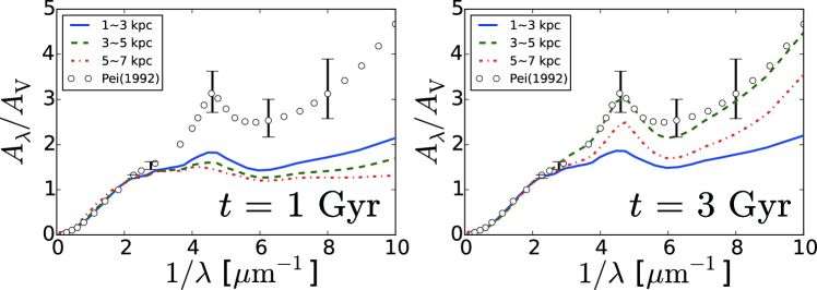
Figure 7: Radial dependence of extinction curves at $t=1$ and 3 Gyr. The blue (solid), green (dashed) and red (dot-dashed) lines correspond to the radial range of $R=1$–3, 3–5, and 5–7 kpc, respectively. We also compare the calculated extinction curves with the same observational data as in Fig. 6.

We investigate the dependence of extinction curves on the galactic radius in a way similar to Hou et al. (2017), who performed the analyses based on our previous simulation with the two-size approximation. Following their paper, we adopt a galactic-radius bin width of 2 kpc and take the mass-weighted average for all gas particles in each radius bin. In order to focus on the extinction curves in the disk region, we exclude the central 1 kpc region. Indeed, the metallicity in the central 1 kpc region is relatively high $Z\gtrsim 3$ Z_☉ (see in fig. 6 of Shimizu et al., 2019) and HA19 also excluded the very central region ($R<0.1$ kpc) for estimating the extinction curves. We analyse the extinction curves up to $R=7$ kpc. Fig. 7 shows the extinction curves in the three radial bins at $t=1$ and 3 Gyr.

We observe in Fig. 7 that the features of extinction curves (the 2175 Å bump and the UV slope) become more prominent with age, which is caused by the increase of small grains relative to large grains. Small grains are more efficiently produced by shattering and accretion at small $R$ in the early epoch as mentioned in Section 3.2.2. As the dust-rich regions extends to the outer radii with age, shattering and accretion become efficient there; thus, the outer regions also have steep extinction curves at $t=3$ Gyr. We give more detailed descriptions in what follows.

At $t=1$ Gyr, the extinction curves at $R<3\,{\rm kpc}$ show a prominent 2175 Å bump and UV rise. The extinction curves at $R>3$ kpc are still flat because the dust abundance is dominated by large grains produced by stars. The radial variation of extinction curves at 3 Gyr shows the opposite trend to that at 1 Gyr, with the outer regions ($R>3$ kpc) having steeper extinction curves compared with the inner regions ($R<$ 3 kpc). In this epoch, accretion dominates the dust evolution in the entire galaxy regions as mentioned above. Therefore, extinction curves have steep slopes in the UV. As discussed in Section 3.1.2, coagulation becomes efficient in the central part, so that the extinction curves are flattened at $R<3$ kpc. The extinction curves are the steepest in the intermediate radii ($R\sim 3$–5 kpc) since accretion is efficient but coagulation is not yet active there. At larger radii ($R>5$ kpc), the extinction curves are flatter because of less efficient accretion.

4 Discussion

4.1 Total dust abundance

Although the main focus of this paper is the grain size distribution, the model should reproduce the evolution of the total dust abundance. In Section 3.2, we have shown that our simulation reproduces the total dust abundance (dust-to-gas ratio) in nearby galaxies. The relation between dust-to-gas ratio and metallicity and the radial profiles of dust-to-gas ratio and dust-to-metal ratio are broadly consistent with the observational data of nearby galaxies.

However, there are some improvements necessary for better agreement with the observational data. In Section 3.2.2, we find that the radial profile of dust-to-metal ratio tends to be above the observational data points, although it is not completely discrepant from the observational data. This raises the following discussions in the early and late epochs. In the early epoch at $t=0.3$ Gyr, the possible discrepancy is due to the overestimate of dust condensation efficiency in stellar ejecta, for which we adopted $f_{\mathrm{in}}=0.1$. In fact, the condensation efficiency is still uncertain: for SNe, the dust mass injected to the ISM is strongly affected by the reverse shock destruction, which is sensitive to the density of the ambient medium (Bianchi & Schneider, 2007; Nozawa et al., 2007). For the dust yield in AGB stars, there are still some variety among different condensation calculations as compiled by Inoue (2011) and Kuo et al. (2013). Considering such uncertainties, the agreement within a factor of 2 is good enough. Moreover, the almost flat slope is consistent with the observational data, which suggests that the stellar dust production is dominant at all galactic radii.

At $t\gtrsim 1$ Gyr, the radial profile of dust-to-metal ratio has a negative gradient, because dust growth by accretion starts to play a role from the central part. The existence of such a negative gradient is consistent with the observational data. However, the calculated radial profiles may be too flat compared with the observational data (see Fig. 5). The flat radial profile is due to efficient dust growth by accretion up to the large galactic radii; thus, accretion is probably too efficient in our calculation. There are some possible improvements for the treatment of accretion. We equally treated all metal elements but dust has some specific composition. Ideally, we should model accretion so that it reproduces the actual dust composition (such as silicate). Hou et al. (2017) treated two grain species (silicate and carbonaceous dust) separately by neglecting a formation of compound species. This is also a simplification, and it may underestimate the accretion efficiency because each grain species accretes only specific elements. Separating the grain species is also important for the prediction of extinction curves. In the future, we will work on a framework that separates the grain species.

4.2 Robustness and uncertainty in the grain size distribution

The shape of grain size distribution is determined by the stellar dust production in the early (or low-metallicity) phase of galaxy evolution. Thus, as long as stars predominantly produce large ($a\gtrsim 0.1\,\micron$) grains, the resulting grain size distribution and extinction curve are robust. As mentioned in the Introduction, most theoretical calculations of dust condensation in stellar ejecta indicate that such large grains are favourably produced.

The grain size distribution in later epochs, on the other hand, is determined by interstellar processing. In our model, shattering plays an important role in the initial production of small grains. As mentioned in Section 2.2.3, it is essential that the largest grains have velocities high enough for shattering ($\gtrsim$ a few km s^-1) in the diffuse ISM. Otherwise, the initial production of small grains does not occur efficiently. Subsequently, accretion and coagulation are important in increasing small and large grains, respectively. The final shape of the grain size distribution approaches the one similar to the MRN grain size distribution. Collisional processes such as coagulation are shown to robustly lead to a grain size distribution like MRN (e.g. Dohnanyi, 1969; Williams & Wetherill, 1994; Tanaka et al., 1996; Kobayashi & Tanaka, 2010). The upper limit of the grain radii is rather sensitive to the subgrid model of coagulation as shown in HA19. If the maximum grain radius becomes as large as $\sim 1\,\micron$, the extinction curve becomes too flat to explain the Milky Way curve. Although $\micron$-sized grains should exist in some dense molecular cloud cores (Pagani et al., 2010; Lefèvre et al., 2014), such large grains should not be the majority of the ISM (see also Draine, 2009). To determine the maximum grain size without any subgrid model, it is necessary to spatially resolve dense molecular cloud cores. This is challenging at this moment, because the simulation box should be wide enough to cover a representative region of a galaxy (i.e. $\sim$kpc scale) but it should still resolve the sub-pc scales. Nevertheless, we could argue that our subgrid model is successful because the maximum grain radius is consistent with MRN ($\sim 0.25~{}\micron$) at $t=3$ Gyr (Fig. 1).

4.3 Importance of implementing dust evolution in hydrodynamic simulations

As mentioned above, direct implementation of dust evolution calculations in hydrodynamic simulations is important since some grain evolution processes occur on short time-scales. According to equation (12), accretion occurs on a time-scale shorter than $10^{7}$ yr for small grains in solar-metallicity environments. The post-processing analysis by HA19 was based on snapshots with intervals of $\sim 10^{7}$ yr, which is too long to capture the change of physical conditions (density and temperature) for accretion. Coagulation also occurs on a comparable time-scale in a solar-metallicity environment. Thus, it is essential to solve the dust evolution and hydrodynamics simultaneously and consistently.

In our simulation, individual SNe cannot be resolved; thus, the rate of SNe affecting a certain gas particle ($\gamma$ in equation 10) is used to estimate the dust destruction rate at each time step. Since SN destruction counteracts the increase of dust mass by accretion which could also have a short time-scale, post-processing does not give precise results. Moreover, the physical condition of the ISM changes rapidly when the SN energy is deposited, and the lifetime of superbubbles is as short as $\sim 10^{6}$ yr (e.g. Draine, 2011). To correctly trace the dust processing induced by the energy input from SNe, we need to solve the grain evolution and hydrodynamics simultaneously.

4.4 Dependence on the subgrid treatment

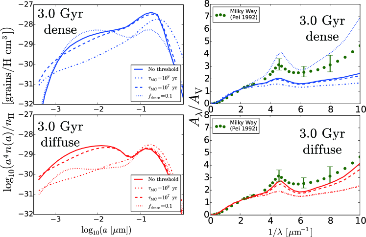
Figure 8: Some additional tests for the subgrid treatment of accretion and coagulation. We show the grain size distributions (left) and extinction curves (right) in the dense (upper) and diffuse (lower) gas particles at $t=3$ Gyr. We only show the medians. The solid line shows our ‘default’ simulation, which is the same as in Figs. 1 and 6. The dashed and dot–dashed lines correspond to the cases with molecular cloud lifetime of $\tau_{\mathrm{MC}}=10^{7}$ and $10^{8}$ yr, respectively (see text). The dotted lines represent the case of a different dust condensation efficiency $f_{\rm dense}=0.1$ without imposing the lifetime of molecular clouds. In the right-bottom panel (extinction curves), the dot–dashed and dotted lines overlap with each other.

In our simulations, the dust processing in dense clouds (accretion and coagulation) is treated by subgrid modelling, because the typical size of dense clouds (or molecular clouds) is much smaller than the typical softening length of gas particles ($\sim$80 pc). Therefore, it is worth examining the robustness of the results by performing additional simulations. We first examine the dependence on $f_{\mathrm{dense}}$ by lowering it to 0.1 (the fiducial value is 0.5). We also test the effect of molecular cloud lifetime, which is determined by the gas dynamical evolution on subgrid scales. We only show the results at $t=3$ Gyr, when the effects of accretion and coagulation appear most significantly among the ages chosen above.

First, we show the results with $f_{\mathrm{dense}}=0.1$ in Fig. 8. We only show the medians. We observe that, compared with the fiducial case with $f_{\mathrm{dense}}=0.5$, the small-grain abundance is enhanced while the large-grain abundance is suppressed in the dense regions. The grain size distribution stays bimodal because coagulation is too weak to create a smooth grain size distribution. Accordingly, the extinction curves become steeper in the dense medium. In the diffuse medium, on the other hand, the abundance of grains with $a\sim 0.01~{}\micron$ is less for the case of smaller $f_{\mathrm{dense}}$. Accordingly, the extinction curves are flat in the diffuse ISM. Recalling that accretion and coagulation dominate the shaping of grain size distribution at a later stage, low $f_{\mathrm{dense}}$ indicates that the evolution of grain size distribution occurs slowly. This explains the difference between $f_{\mathrm{dense}}=0.5$ and 0.1.

Next, we examine the effect of molecular cloud lifetime. We implicitly assumed that the mass exchange between molecular clouds and other gas is frequent enough so that the uniform grain size distribution is achieved on the subgrid scale. However, if such an exchange does not occur, dust growth by accretion could be saturated in each molecular cloud. In this case, accretion is regulated by the lifetime of molecular clouds rather than the actual accretion time-scale (Hirashita, 2000). To examine this effect, we set $\tau_{\mathrm{acc}}=\tau_{\mathrm{MC}}$ if $\tau_{\mathrm{acc}}$ (equation 12) is shorter than $\tau_{\mathrm{MC}}$ (molecular cloud lifetime). The lifetime of molecular clouds are uncertain, but it is likely to be on the order of $10^{7}$ yr (Ward-Thompson et al., 2006; Bergin & Tafalla, 2007). Koda et al. (2009) suggested longer lifetimes ($\sim 10^{8}$ yr) based on the observed stability of dense structures. Thus, we examine $\tau_{\mathrm{MC}}=10^{7}$ yr and $10^{8}$ yr. Since $\tau_{\mathrm{acc}}$ estimated by equation (12) is inversely proportional to the metallicity, $\tau_{\mathrm{acc}}=\tau_{\mathrm{MC}}$ is adopted only if the metallicity is high enough. Coagulation has no saturation; therefore we only change the prescription for accretion here.

The result for $\tau_{\mathrm{MC}}=10^{7}$ yr is shown in Fig. 8. We observe that, if $\tau_{\mathrm{MC}}=10^{7}$ yr, the results do not change much for the grain size distribution and extinction curves. This means that the accretion time-scale is mostly longer than $10^{7}$ yr (i.e. $\tau_{\mathrm{acc}}>\tau_{\mathrm{MC}}$ in most of the cases so that $\tau_{\mathrm{acc}}=\tau_{\mathrm{MC}}$ is rarely adopted). In contrast, if $\tau_{\mathrm{MC}}=10^{8}$ yr, the abundance of grains at $a\lesssim 10^{-1.5}\,\mu{\rm m}$ is significantly suppressed. This is because of less efficient accretion. If $\tau_{\mathrm{MC}}$ is as long as $10^{8}$ yr, $\tau_{\mathrm{acc}}$ estimated by equation (12) more often becomes shorter than $\tau_{\mathrm{MC}}$ (i.e. $\tau_{\mathrm{acc}}=\tau_{\mathrm{MC}}$ is more often adopted). We also observe that the abundance of the biggest grains is higher for this case because large grains are shattered less by small grains. Because of the dominance of large grains, extinction curves are very flat in both dense and diffuse media.

In summary, the subgrid treatment of accretion and coagulation affects the results. The fraction of dense gas (or the structure of gas density below a few ${}\times 10$ pc) and the molecular cloud lifetime are particularly important. It is desirable to determine or constrain these quantities by higher-resolution simulations and/or observations.

4.5 Future prospect

In this paper, we only simulated an isolated disc galaxy. Although we expect that this work gives a representative case for dust evolution, there are clearly other types of galaxies with various star formation time-scales and mass scales. To calculate the evolution of various types of galaxies, cosmological simulations would be ideal. Therefore, a natural extension of this work is to implement the evolution of full grain size distribution in cosmological hydrodynamic simulations. Since cosmological calculations have worse spatial resolution, the calculation results in this paper will give a useful calibration for similar galaxies produced in a cosmological box.

Cosmological zoom-in simulations that focus on some specific halos are also useful to achieve a high spatial resolution. There are some examples of such simulations using zoom-in methods (Yajima et al., 2015; McKinnon et al., 2016) which revealed the dust distribution in galaxies. In particular, high spatial resolution is important to predict detailed radiative properties since the wavelength dependence of dust absorption at UV and optical wavelengths in the entire galaxy (i.e. the attenuation curve) depends not only on the extinction curve but also on the spatial distribution of dust and stars (e.g. Calzetti, 2001; Inoue, 2005; Narayanan et al., 2018b). However, we would also like to predict the statistical properties of galaxies at different redshifts, and for this, a full cosmological simulation with a large box size is more desired, in addition to the limited galaxy sample in zoom-in simulations.

Recently, Aoyama et al. (2019) calculated the dust emission properties by post-processing their cosmological simulation. Because of low spatial resolution, they applied a one-zone calculation for the radiative properties. They succeeded in predicting the statistical properties of dust emission such as the IR luminosity function, IRX–$\beta$ (IR-to-UV luminosity ratio vs. UV spectral slope) relation, etc. Indeed, for the IRX–$\beta$ relation, the extinction curve (more precisely, attenuation curve; Narayanan et al. 2018a) is important. Since Aoyama et al. (2019) adopted the two-size approximation, their extinction curves only had two degrees of freedom, so that their predictive power of extinction curves was limited. By calculating the full grain-size distribution in the future, we will obtain a better prediction for extinction curves also in cosmological simulations.

5 Conclusion

We performed a hydrodynamic simulation of an isolated disc galaxy with the evolution of full grain size distribution. We solved the time evolution of grain size distribution caused by stellar dust production, SN destruction, shattering, accretion, and coagulation on each gas (SPH) particle in the gadget3-osaka hydrodynamic simulation. Each of the dust evolution processes above is treated in a consistent manner with the local physical conditions (gas density, temperature, metallicity, etc.) of the gas particle. As a consequence, we obtain the spatially resolved information on the grain size distribution at each stage of galaxy evolution.

For the total dust abundance, our simulation reproduces the relation between dust-to-gas ratio and metallicity, as well as the radial profiles of dust-to-gas ratio and dust-to-metal ratio in nearby galaxies. We also confirm that the obtained results for the total dust amount is consistent with our previous simulation (A17) which adopted the two-size approximation. Therefore, we conclude that our models give reasonable results as far as the total dust abundance is concerned.

For the evolution of grain size distribution, we obtain the following results, taking advantage of the spatially resolved information. The grain size distribution is dominated by large grains in the earliest phase ($t\lesssim 0.3$ Gyr) in the entire disc. In the intermediate stage ($t\sim 1$ Gyr), small grains are more abundant in the dense, metal-enriched ISM, where shattering and accretion can efficiently form a bump (second peak) at $a\sim 0.01\,\mu$m. Therefore, the extinction curves are steeper in the dense ISM than in the diffuse ISM. At a later stage ($t\gtrsim 3$ Gyr), the relative abundance of small grains to large grains is higher in the diffuse ISM than in the dense ISM. This is because higher dust abundances in the dense ISM are favourable for coagulation, which creates large grains by depleting small grains. Accordingly, the extinction curve becomes flatter in the dense ISM at later times. The grain size distribution approaches to the MRN distribution at $t\gtrsim 3$ Gyr, and the Milky Way extinction curve is reproduced well.

The grain size distribution depends also on the position in the galaxy. At young ages ($t\lesssim 1$ Gyr), the small-grain abundance is most enhanced in the central region (at small galactic radii $R$). This is because the highest dust abundance in the central part leads to the most active shattering and accretion. In contrast, the small-grain abundance is the lowest at small $R$ at a later stage ($t\gtrsim 3$ Gyr) because of coagulation. Accordingly, extinction curves are the steepest at small $R$ at young ($t\lesssim 1$ Gyr) ages, while they are the flattest at small $R$ at old ($t\gtrsim 3$ Gyr) ages. Since the above change in the grain size distribution occurs at $t\sim 1$ Gyr, the age and density dependence of grain size distribution has a significant impact on the extinction curves even at high redshift.

We emphasize that all the above results are consistent with the results obtained by our simpler grain evolution model using the two-size approximation (e.g. Aoyama et al., 2018; Hou et al., 2019; Aoyama et al., 2019). This not only indicates the robustness of the results in this paper but also supports our previous results. We should, however, emphasize that the full grain size distribution is essential in predicting observable quantities such as extinction curves and dust emission properties (radiation transfer effects).

References

- Aoyama et al. (2017) Aoyama S., Hou K.-C., Shimizu I., Hirashita H., Todoroki K., Choi J.-H., Nagamine K., 2017, MNRAS, 466, 105
- Aoyama et al. (2018) Aoyama S., Hou K.-C., Hirashita H., Nagamine K., Shimizu I., 2018, MNRAS, 478, 4905
- Aoyama et al. (2019) Aoyama S., et al., 2019, MNRAS, 484, 1852
- Asano et al. (2013a) Asano R. S., Takeuchi T. T., Hirashita H., Inoue A. K., 2013a, Earth, Planets, and Space, 65, 213
- Asano et al. (2013b) Asano R. S., Takeuchi T. T., Hirashita H., Nozawa T., 2013b, MNRAS, 432, 637
- Bekki (2015) Bekki K., 2015, MNRAS, 449, 1625
- Bergin & Tafalla (2007) Bergin E. A., Tafalla M., 2007, ARA&A, 45, 339
- Bianchi & Schneider (2007) Bianchi S., Schneider R., 2007, MNRAS, 378, 973
- Bohren & Huffman (1983) Bohren C. F., Huffman D. R., 1983, Absorption and scattering of light by small particles. A Wiley-Interscience Publication
- Buat & Xu (1996) Buat V., Xu C., 1996, A&A, 306, 61
- Calzetti (2001) Calzetti D., 2001, PASP, 113, 1449
- Casuso & Beckman (2012) Casuso E., Beckman J. E., 2012, MNRAS, 419, 1642
- Cazaux & Tielens (2004) Cazaux S., Tielens A. G. G. M., 2004, ApJ, 604, 222
- Chen et al. (2018) Chen L.-H., Hirashita H., Hou K.-C., Aoyama S., Shimizu I., Nagamine K., 2018, MNRAS, 474, 1545
- Chiang et al. (2018) Chiang I. D., Sandstrom K. M., Chastenet J., Johnson L. C., Leroy A. K., Utomo D., 2018, ApJ, 865, 117
- Dayal et al. (2010) Dayal P., Hirashita H., Ferrara A., 2010, MNRAS, 403, 620
- De Vis et al. (2019) De Vis P., et al., 2019, A&A, 623, A5
- de Bennassuti et al. (2014) de Bennassuti M., Schneider R., Valiante R., Salvadori S., 2014, MNRAS, 445, 3039
- Dell’Agli et al. (2017) Dell’Agli F., García-Hernández D. A., Schneider R., Ventura P., La Franca F., Valiante R., Marini E., Di Criscienzo M., 2017, MNRAS, 467, 4431
- Dohnanyi (1969) Dohnanyi J. S., 1969, J. Geophys. Res., 74, 2531
- Draine (2009) Draine B. T., 2009, Space Sci. Rev., 143, 333
- Draine (2011) Draine B. T., 2011, Physics of the Interstellar and Intergalactic Medium. Princeton University Press
- Dwek (1998) Dwek E., 1998, ApJ, 501, 643
- Elmegreen (1998) Elmegreen D. M., 1998, Galaxies and galactic structure. Upper Saddle River, NJ : Prentice Hall
- Ferrarotti & Gail (2006) Ferrarotti A. S., Gail H.-P., 2006, A&A, 447, 553
- Fitzpatrick & Massa (2007) Fitzpatrick E. L., Massa D., 2007, ApJ, 663, 320
- Ginolfi et al. (2018) Ginolfi M., Graziani L., Schneider R., Marassi S., Valiante R., Dell’Agli F., Ventura P., Hunt L. K., 2018, MNRAS, 473, 4538
- Gjergo et al. (2018) Gjergo E., Granato G. L., Murante G., Ragone-Figueroa C., Tornatore L., Borgani S., 2018, MNRAS, 479, 2588
- Graziani et al. (2019) Graziani L., Schneider R., Ginolfi M., Hunt L. K., Maio U., Glatzle M., Ciardi B., 2019, arXiv e-prints, p. arXiv:1909.07388
- Guillet et al. (2011) Guillet V., Pineau Des Forêts G., Jones A. P., 2011, A&A, 527, A123
- Hirashita (1999a) Hirashita H., 1999a, ApJ, 510, L99
- Hirashita (1999b) Hirashita H., 1999b, ApJ, 522, 220
- Hirashita (2000) Hirashita H., 2000, PASJ, 52, 585
- Hirashita (2012) Hirashita H., 2012, MNRAS, 422, 1263
- Hirashita (2015) Hirashita H., 2015, MNRAS, 447, 2937
- Hirashita & Aoyama (2019) Hirashita H., Aoyama S., 2019, MNRAS, 482, 2555
- Hirashita & Ferrara (2002) Hirashita H., Ferrara A., 2002, MNRAS, 337, 921
- Hirashita & Kobayashi (2013) Hirashita H., Kobayashi H., 2013, Earth, Planets, and Space, 65, 1083
- Hirashita & Voshchinnikov (2014) Hirashita H., Voshchinnikov N. V., 2014, MNRAS, 437, 1636
- Hirashita & Yan (2009) Hirashita H., Yan H., 2009, MNRAS, 394, 1061
- Hopkins & Lee (2016) Hopkins P. F., Lee H., 2016, MNRAS, 456, 4174
- Hou et al. (2016) Hou K.-C., Hirashita H., Michałowski M. J., 2016, PASJ, 68, 94
- Hou et al. (2017) Hou K.-C., Hirashita H., Nagamine K., Aoyama S., Shimizu I., 2017, MNRAS, 469, 870
- Hou et al. (2019) Hou K.-C., Aoyama S., Hirashita H., Nagamine K., Shimizu I., 2019, MNRAS, 485, 1727
- Hu et al. (2019) Hu C.-Y., Zhukovska S., Somerville R. S., Naab T., 2019, MNRAS, 487, 3252
- Inoue (2003) Inoue A. K., 2003, PASJ, 55, 901
- Inoue (2005) Inoue A. K., 2005, MNRAS, 359, 171
- Inoue (2011) Inoue A. K., 2011, Earth, Planets, and Space, 63, 1027
- Inoue et al. (2000) Inoue A. K., Hirashita H., Kamaya H., 2000, PASJ, 52, 539
- Jones et al. (1994) Jones A. P., Tielens A. G. G. M., Hollenbach D. J., McKee C. F., 1994, ApJ, 433, 797
- Jones et al. (1996) Jones A. P., Tielens A. G. G. M., Hollenbach D. J., 1996, ApJ, 469, 740
- Kennicutt & Evans (2012) Kennicutt R. C., Evans N. J., 2012, ARA&A, 50, 531
- Kennicutt et al. (2003) Kennicutt R. C., et al., 2003, PASP, 115, 928
- Kim et al. (2014) Kim J.-h., et al., 2014, ApJS, 210, 14
- Kim et al. (2016) Kim J.-h., et al., 2016, ApJ, 833, 202
- Kobayashi & Tanaka (2010) Kobayashi H., Tanaka H., 2010, Icarus, 206, 735
- Koda et al. (2009) Koda J., et al., 2009, The Astrophysical Journal, 700, L132
- Kozasa et al. (1989) Kozasa T., Hasegawa H., Nomoto K., 1989, ApJ, 344, 325
- Kuo & Hirashita (2012) Kuo T.-M., Hirashita H., 2012, MNRAS, 424, L34
- Kuo et al. (2013) Kuo T.-M., Hirashita H., Zafar T., 2013, MNRAS, 436, 1238
- Lefèvre et al. (2014) Lefèvre C., et al., 2014, A&A, 572, A20
- Li et al. (2019) Li Q., Narayanan D., Davé R., 2019, MNRAS, 490, 1425
- Lisenfeld & Ferrara (1998) Lisenfeld U., Ferrara A., 1998, ApJ, 496, 145
- Maoz & Mannucci (2012) Maoz D., Mannucci F., 2012, Publ. Astron. Soc. Australia, 29, 447
- Marinacci et al. (2014) Marinacci F., Pakmor R., Springel V., Simpson C. M., 2014, MNRAS, 442, 3745
- Marinacci et al. (2019) Marinacci F., Sales L. V., Vogelsberger M., Torrey P., Springel V., 2019, arXiv e-prints, p. arXiv:1905.08806
- Mathis et al. (1977) Mathis J. S., Rumpl W., Nordsieck K. H., 1977, ApJ, 217, 425
- Mattsson (2016) Mattsson L., 2016, Planetary and Space Science, 133, 107
- Mattsson & Andersen (2012) Mattsson L., Andersen A. C., 2012, MNRAS, 423, 38
- Mattsson et al. (2012) Mattsson L., Andersen A. C., Munkhammar J. D., 2012, MNRAS, 423, 26
- McKee (1989) McKee C., 1989, in Allamandola L. J., Tielens A. G. G. M., eds, IAU Symposium Vol. 135, Interstellar Dust. p. 431
- McKinnon et al. (2016) McKinnon R., Torrey P., Vogelsberger M., 2016, MNRAS, 457, 3775
- McKinnon et al. (2017) McKinnon R., Torrey P., Vogelsberger M., Hayward C. C., Marinacci F., 2017, MNRAS, 468, 1505
- McKinnon et al. (2018) McKinnon R., Vogelsberger M., Torrey P., Marinacci F., Kannan R., 2018, MNRAS, 478, 2851
- Moustakas et al. (2010) Moustakas J., Kennicutt Jr. R. C., Tremonti C. A., Dale D. A., Smith J.-D. T., Calzetti D., 2010, ApJS, 190, 233
- Muñoz-Mateos et al. (2009) Muñoz-Mateos J. C., et al., 2009, ApJ, 703, 1569
- Narayanan et al. (2018a) Narayanan D., Davé R., Johnson B. D., Thompson R., Conroy C., Geach J., 2018a, MNRAS, 474, 1718
- Narayanan et al. (2018b) Narayanan D., Conroy C., Davé R., Johnson B. D., Popping G., 2018b, ApJ, 869, 70
- Nozawa & Fukugita (2013) Nozawa T., Fukugita M., 2013, ApJ, 770, 27
- Nozawa et al. (2003) Nozawa T., Kozasa T., Umeda H., Maeda K., Nomoto K., 2003, ApJ, 598, 785
- Nozawa et al. (2007) Nozawa T., Kozasa T., Habe A., Dwek E., Umeda H., Tominaga N., Maeda K., Nomoto K., 2007, ApJ, 666, 955
- Omukai et al. (2005) Omukai K., Tsuribe T., Schneider R., Ferrara A., 2005, ApJ, 626, 627
- Ormel et al. (2009) Ormel C. W., Paszun D., Dominik C., Tielens A. G. G. M., 2009, A&A, 502, 845
- Pagani et al. (2010) Pagani L., Steinacker J., Bacmann A., Stutz A., Henning T., 2010, Science, 329, 1622
- Pei (1992) Pei Y. C., 1992, ApJ, 395, 130
- Popping et al. (2017) Popping G., Somerville R. S., Galametz M., 2017, MNRAS, 471, 3152
- Rémy-Ruyer et al. (2014) Rémy-Ruyer A., et al., 2014, A&A, 563, A31
- Saitoh (2017) Saitoh T. R., 2017, AJ, 153, 85
- Saitoh et al. (2008) Saitoh T. R., Daisaka H., Kokubo E., Makino J., Okamoto T., Tomisaka K., Wada K., Yoshida N., 2008, PASJ, 60, 667
- Schneider et al. (2006) Schneider R., Omukai K., Inoue A. K., Ferrara A., 2006, MNRAS, 369, 1437
- Shimizu et al. (2019) Shimizu I., Todoroki K., Yajima H., Nagamine K., 2019, MNRAS, 484, 2632
- Springel (2005) Springel V., 2005, MNRAS, 364, 1105
- Springel (2010) Springel V., 2010, MNRAS, 401, 791
- Takeuchi et al. (2005) Takeuchi T. T., Buat V., Burgarella D., 2005, A&A, 440, L17
- Tanaka et al. (1996) Tanaka H., Inaba S., Nakazawa K., 1996, Icarus, 123, 450
- Todini & Ferrara (2001) Todini P., Ferrara A., 2001, MNRAS, 325, 726
- Totani et al. (2008) Totani T., Morokuma T., Oda T., Doi M., Yasuda N., 2008, PASJ, 60, 1327
- Ventura et al. (2014) Ventura P., Dell’Agli F., Schneider R., Di Criscienzo M., Rossi C., La Franca F., Gallerani S., Valiante R., 2014, MNRAS, 439, 977
- Vijayan et al. (2019) Vijayan A. P., Clay S. J., Thomas P. A., Yates R. M., Wilkins S. M., Henriques B. M., 2019, MNRAS, 489, 4072
- Wada & Norman (2007) Wada K., Norman C. A., 2007, ApJ, 660, 276
- Ward-Thompson et al. (2006) Ward-Thompson D., Nutter D., Bontemps S., Whitworth A., Attwood R., 2006, MNRAS, 369, 1201
- Weingartner & Draine (2001) Weingartner J. C., Draine B. T., 2001, ApJ, 548, 296
- Williams & Wetherill (1994) Williams D. R., Wetherill G. W., 1994, Icarus, 107, 117
- Yajima et al. (2015) Yajima H., Shlosman I., Romano-Díaz E., Nagamine K., 2015, MNRAS, 451, 418
- Yamasawa et al. (2011) Yamasawa D., Habe A., Kozasa T., Nozawa T., Hirashita H., Umeda H., Nomoto K., 2011, ApJ, 735, 44
- Yan et al. (2004) Yan H., Lazarian A., Draine B. T., 2004, ApJ, 616, 895
- Yasuda & Kozasa (2012) Yasuda Y., Kozasa T., 2012, ApJ, 745, 159
- Zhukovska (2014) Zhukovska S., 2014, A&A, 562, A76
- Zhukovska et al. (2008) Zhukovska S., Gail H.-P., Trieloff M., 2008, A&A, 479, 453
- Zhukovska et al. (2016) Zhukovska S., Dobbs C., Jenkins E. B., Klessen R. S., 2016, ApJ, 831, 147