On localized and coherent states on some new fuzzy spheres

Abstract

We construct various systems of coherent states (SCS) on the $O(D)$-equivariant fuzzy spheres $S^{d}_{\Lambda}$ ($d=1,2$, $D=d\!+\!1$) constructed in [G. Fiore, F. Pisacane, J. Geom. Phys. 132 (2018), 423-451] and study their localizations in configuration space as well as angular momentum space. These localizations are best expressed through the $O(D)$-invariant square space and angular momentum uncertainties $(\Delta\bm{x})^{2},(\Delta\bm{L})^{2}$ in the ambient Euclidean space $\mathbb{R}^{D}$. We also determine general bounds (e.g. uncertainty relations from commutation relations) for $(\Delta\bm{x})^{2},(\Delta\bm{L})^{2}$, and partly investigate which SCS may saturate these bounds. In particular, we determine $O(D)$-equivariant systems of optimally localized coherent states, which are the closest quantum states to the classical states (i.e. points) of $S^{d}$. We compare the results with their analogs on commutative $S^{d}$. We also show that on $S^{2}_{\Lambda}$ our optimally localized states are better localized than those on the Madore-Hoppe fuzzy sphere with the same cutoff $\Lambda$.

1 Introduction

The present interest in noncommutative space(time) algebras has various motivations. In particular, such algebras may describe spacetimes at microscopic scales, regularizing ultraviolet divergencies in quantum field theory (QFT) and/or allowing the quantization of gravity, or may help to unify fundamental interactions (see e.g. [1, 2, 3, 4, 5]). Noncommutative geometry [6, 7, 8, 9] develops the needed machinery of differential geometry on such algebras. Fuzzy spaces are special examples of noncommutative spaces: a fuzzy space is a sequence $\{\mathcal{A}_{n}\}_{n\in\mathbb{N}}$ of finite-dimensional algebras such that as $n$ diverges $\mathcal{A}_{n}$ goes to the commutative algebra ${\cal A}$ of regular functions on an ordinary manifold. The first and seminal fuzzy space is the socalled Fuzzy 2-Sphere (FS) of Madore and Hoppe [10, 11]: ${\cal A}_{n}\simeq M_{n}(\mathbb{C})$ (the algebra of complex $n\times n$ matrices) is generated by coordinate operators $\left\{x_{i}\right\}_{i=1}^{3}$ fulfilling

$$[x_{i},x_{j}]=\frac{2i}{\sqrt{n^{2}\!-\!1}}\varepsilon^{ijk}x_{k},\qquad\qquad x_{i}x_{i}=1$$ (1)

($n\!>\!1$, sum over repeated indices is understood); in fact these are obtained by the rescaling

$$x_{i}=\frac{2L_{i}}{\sqrt{n^{2}\!-\!1}},\quad i=1,2,3$$ (2)

of the elements $L_{i}$ of the standard basis of $so(3)$ in the irreducible representation $(\pi_{l},V_{l})$ characterized by $\bm{L}^{2}:=L_{i}L_{i}=l(l\!+\!1)$, or equivalently of dimension $n=2l\!+\!1$.

On the contrary, the Hilbert space ${\cal L}^{2}(S^{2})$ of a quantum particle on $S^{2}$ decomposes as the direct sum of all the irreducible representations of $SO(3)$,

$${\cal L}^{2}(S^{2})=\bigoplus\limits_{l=0}^{\infty}V_{l};$$ (3)

the angular momentum components  $L_{i}$  map the generic $V_{l}$ into itself, while the $x_{i}$ map it into $V_{l-1}\oplus V_{l+1}$. Moreover, relations (1) are equivariant under $SO(3)$, but not under the whole $O(3)$, in particular not under parity $x_{i}\mapsto-x_{i}$; whereas the commutators of the cooordinates $x_{i}$ on the sphere $S^{2}$ remain zero under all $O(3)$ transformations.

In [12] we have introduced some new fuzzy approximations of $S^{1},S^{2}$ - more precisely a fully $O(2)$-equivariant fuzzy circle $\{S^{1}_{\Lambda}\}_{\Lambda\in\mathbb{N}}$ and a fully $O(3)$-equivariant fuzzy 2-sphere $\{S^{2}_{\Lambda}\}_{\Lambda\in\mathbb{N}}$;  the latter is free of the mentioned shortcomings. To construct $S^{d}_{\Lambda}$ ($d\!=\!1,2$) we have first projected the Hilbert space $\mathcal{L}^{2}(\mathbb{R}^{D})$ of a zero-spin quantum particle in $\mathbb{R}^{D}$ ($D\!:=\!d\!+\!1$) onto the finite-dimensional subspace $\mathcal{H}_{\Lambda}$ spanned by all the $\psi$ fulfilling

$$H_{\Lambda}\psi=E\psi,\qquad\mbox{where }\quad H_{\Lambda}:=-\frac{1}{2}\Delta+U_{\Lambda}(r),\quad E\leq\overline{E}(\Lambda):=\Lambda(\Lambda\!+\!d\!-\!1).$$ (4)

Here $r^{2}:=\bm{x}^{2}=x_{i}x_{i}$,  $x_{i}$ ($i=1,...,D$) are Cartesian coordinates of $\mathbb{R}^{D}$ (we use dimensionless variables),  $\Delta:=\frac{\partial}{\partial x_{i}}\frac{\partial}{\partial x_{i}}$ is the Laplacian on $\mathbb{R}^{D}$, $U_{\Lambda}(r)$ is a confining potential with a very sharp minimum at $r=1$, i.e. with $U_{\Lambda}^{\prime}(1)=0$ and very large $k(\Lambda):=U_{\Lambda}^{\prime\prime}(1)/4>0$;   we have fixed $U_{\Lambda}(1)$ so that the lowest energy (i.e. eigenvalue of the Hamiltonian $H_{\Lambda}$) is $E_{0}=0$.  In other words, the subspace $\mathcal{H}_{\Lambda}\subset\mathcal{L}^{2}(\mathbb{R}^{D})$ is characterized by energies below the cutoff $\overline{E}$. Passing to the radial coordinate $r$ and angular ones, (4) is reduced to a 1-dimensional Schrödinger equation in an unknown $f(r)$. This is well approximated by that of a harmonic oscillator by further requiring that $U_{\Lambda}$ satisfies the conditions

$$U_{\Lambda}(r)\simeq U_{\Lambda}(1)+2k(r-1)^{2},\qquad\qquad k(\Lambda)\geq\Lambda^{2}(\Lambda\!+\!1)^{2}$$ (5)

(this guarantees in particular that the classically allowed region $U_{\Lambda}(r)\leq\overline{E}$ is a thin spherical shell of radius $\simeq 1$); by the second we also exclude all radial excitations from the part of the spectrum of $H_{\Lambda}$ below $\overline{E}$ and make the latter coincide [up to terms $O(1/\Lambda)$ depending on higher order terms in the Taylor expansion of $V_{\Lambda}$] with that of the Hamiltonian of free motions (the Laplacian) on $S^{d}$, $\bm{L}^{2}:=L_{ij}L_{ij}/2$;  here $L_{ij}:=i(x_{j}\frac{\partial}{\partial x_{i}}\!-\!x_{i}\frac{\partial}{\partial x_{j}})$ are the angular momentum components. Denoting as $P_{\Lambda}$ the projection on $\mathcal{H}_{\Lambda}$, to every observable $A$ on $\mathcal{L}^{2}(\mathbb{R}^{D})$ we can associate one $\overline{A}:=P_{\Lambda}AP_{\Lambda}$ on $\mathcal{H}_{\Lambda}$. In particular we have computed at leading order in $1/\Lambda$ the action of $\overline{x_{i}}$, $\overline{L_{ij}}$ on $\mathcal{H}_{\Lambda}$ and the algebraic relations that they fulfill. We have fine-tuned the definition of the “fuzzy” Cartesian coordinates $\overline{x_{i}}$ and angular momentum components $\overline{L_{ij}}$ in the simplest way, allowed by the residual freedom of choice of $V_{\Lambda}$; these relations are reported at the beginnings of sections 3, 4. The resulting algebra $\mathcal{A}_{\Lambda}=End(\mathcal{H}_{\Lambda})$ of fuzzy observables is equivariant under the full group $O(D)$ of orthogonal transformations (including inversions of the axes), is generated by the $\overline{x_{i}}$ and is spanned by ordered monomials in $\overline{x_{i}}$, $\overline{L_{ij}}$.  In particular  $[\overline{x_{i}},\overline{x_{j}}]$   is proportional to $\overline{L_{ij}}$, as in Snyder noncommutative space [13] and in some higher dimensional fuzzy spheres [14, 15, 16, 17]. Actually, there is an $O(D)$-equivariant realization of $\mathcal{A}_{\Lambda}$ in terms of an irreducible vector representation of $Uso(D+1)$: the $\overline{L_{ij}}$ are realized exactly as the elements  $L_{ij}\!\in\!so(D)\!\subset\!so(D+1)$,  while the $\overline{x_{i}}$ are realized as the elements  $L_{(D+1)i}\!\in\!so(D+1)$  multiplied by factors depending only on $\bm{L}^{2}$. Below we shall remove the bar and denote $\overline{x_{i}}$, $\overline{L_{ij}}$ again as $x_{i},L_{ij}$. Moreover, the Hilbert space $\mathcal{H}_{\Lambda}$ on $S^{2}_{\Lambda}$ decomposes as the direct sum  $\mathcal{H}_{\Lambda}=\bigoplus\nolimits_{l=0}^{\Lambda}V_{l}$;  the angular momentum components  $L_{i}=\varepsilon^{ijk}L_{jk}/2$  map the generic $V_{l}$ into itself, while the coordinates $x_{i}$ map it into $V_{l-1}\oplus V_{l+1}$, as they do on ${\cal L}^{2}(S^{2})=\bigoplus_{l=0}^{\infty}V_{l}$. For these reasons we believe that in the $\Lambda\!\to\!\infty$ limit the fuzzy sphere $S^{2}_{\Lambda}$ approximates the configuration space $S^{2}$ better than the FS does.

As known [18, 19, 20, 21], systems of coherent states (SCS) are an extremely useful tool for studying quantum theories with both finitely and infinitely many degrees of freedom (QFT). In particular, they may decisively simplify the computation of path integrals representing propagators, correlation functions and their generating functionals; this is applied in nuclear, atomic, condensed matter and elementary particle physics (see e.g. [22, 23, 24, 25]). From a foundation-minded viewpoint, Berezin’s quantization procedure on Kähler manifolds [26, 27, 28] itself is based on the existence of SCS. For the same reasons the search for coherent states is crucial [29, 30] also for quantum theories on fuzzy manifolds (see e.g. [31, 2, 14, 5, 32]). Standard SCS $\{|\alpha\rangle\}_{\alpha\in\mathbb{C}}$ on the phase plane can be defined in 3 equivalent ways:

(A) $|\alpha\rangle$ saturates Heisenberg uncertainty relation (HUR).

(B) $|\alpha\rangle$ is an eigenstate of the annihilation operator with eigenvalue $\alpha\in\mathbb{C}$.

(C) $|\alpha\rangle$ is generated by the Heisenberg-Weyl group operator $D(\alpha)$ acting on vacuum $|0\rangle$.

Perelomov [21, 33] defines generalized CS on orbits of various Lie groups $G$ basically using (C); $|0\rangle$ can be any vector in the carrier Hilbert space. If $|0\rangle$ maximizes the isotropy subalgebra $\mathfrak{b}$ in the complex hull of the Lie algebra of $G$, then it is also annihilated by some element(s) in $\mathfrak{b}$, the corresponding CS are eigenvectors of the latter and minimize a specific $G$-invariant uncertainty [$(\Delta\bm{L})^{2}$ in the case $G=SO(D)$, see below]; in this sense also properties (A), (B) are fulfilled.

The main aim of the present work is to introduce on $S^{d}_{\Lambda}$ ($d=1,2$) various systems of coherent states (SCS). We follow in spirit Perelomov’s approach, with $G$ the isometry group $O(D)$ of $S^{d}$. However, our Hilbert space $\mathcal{H}_{\Lambda}$ will in general carry a reducible representation of $O(D)$; moreover, we study the localization properties of these SCS also in configuration space, beside in (angular) momentum space. We consider SCS both in the strong sense, i.e. providing a resolution of the identity, and in the weak sense, i.e. making up just an (over)complete set in ${\cal H}_{\Lambda}$. On $\mathcal{H}_{\Lambda}$ the uncertainties $\Delta x_{i},\Delta L_{ij}$ must fulfill a number of uncertainty relations and other inequalities following from the algebraic relations (commutation, etc.) among the $x_{i},L_{ij}$. Neither on the commutative nor on the fuzzy spheres is it possible to saturate all of them (and their consequences, a fortiori). Therefore we preliminarly discuss the saturation of suitable $O(D)$-invariant inequalities first on $S^{d}$, then on $S^{d}_{\Lambda}$ , because they have a physical meaning independent of the particular chosen reference frame, and because a state saturating them is automatically mapped into another one by the unitary transformation $U(g)$ corresponding to any orthogonal transformation $g\in O(D)$  [by definition $g_{ij}x_{j}=U^{-1}(g)\,x_{i}\,U(g)$, etc.].

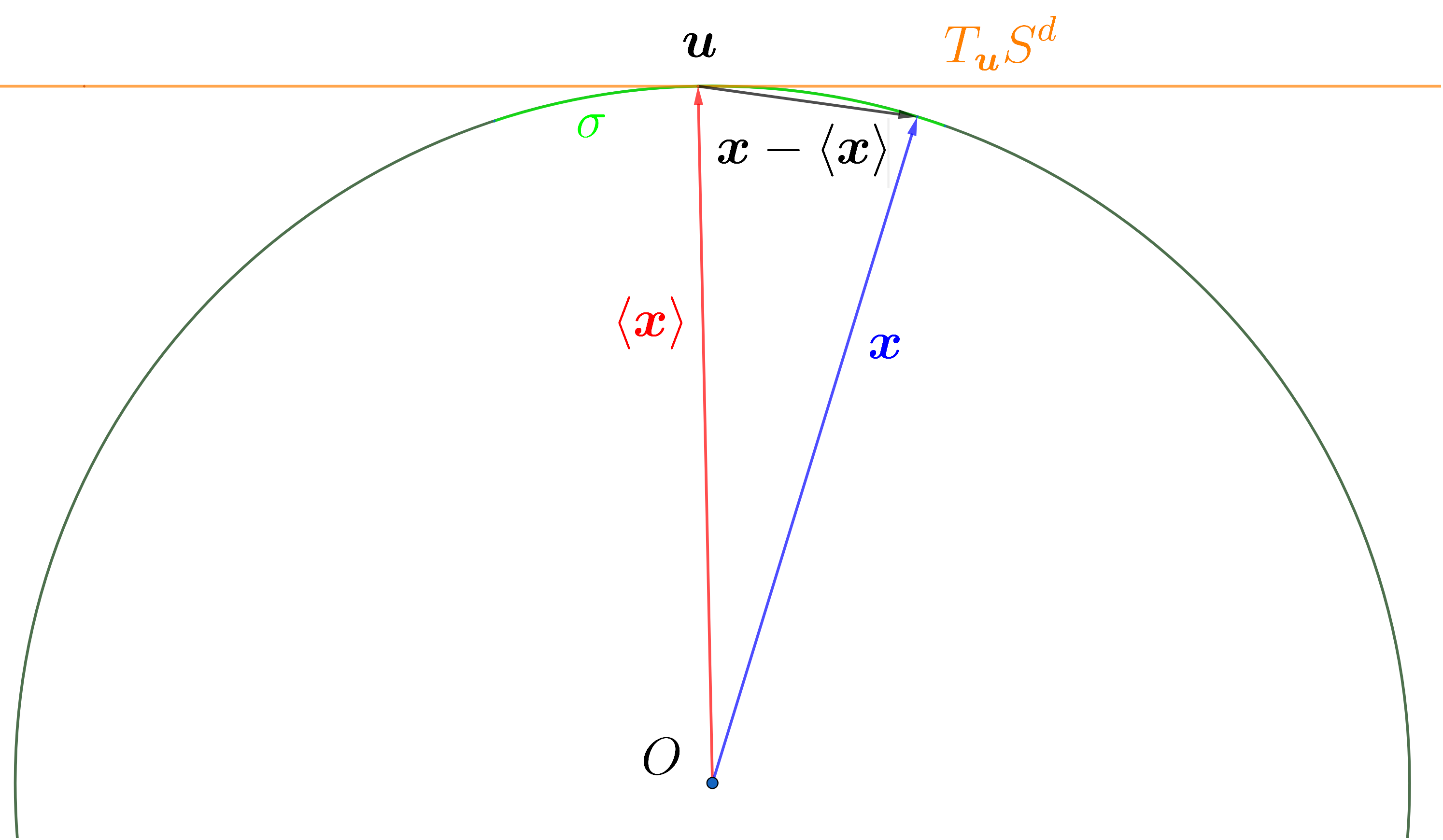
Figure 1: The vectors $\bm{x}$, $\left\langle\bm{x}\right\rangle$, $\bm{x}-\left\langle\bm{x}\right\rangle$, the region $\sigma$ and the tangent plane $T_{\bm{u}}S^{d}$ at $\bm{u}$.

More precisely, as a measure of localization of a state in configuration space we adopt its spacial dispersion, i.e. the expectation value

$$(\Delta\bm{x})^{2}:=\sum_{i=1}^{D}(\Delta x_{i})^{2}\equiv\left\langle\left(\bm{x}\!-\!\left\langle\bm{x}\right\rangle\right)^{2}\right\rangle=\left\langle\bm{x}\,{}^{2}\right\rangle-\left\langle\bm{x}\right\rangle^{2}$$ (7)

on the state; here $\bm{x}\equiv(x_{1},...,x_{n})$, $\left\langle\bm{x}\right\rangle\equiv(\left\langle x_{1}\right\rangle,...,\left\langle x_{n}\right\rangle)$ pinpoints the average position of the particle in the ambient Euclidean space $\mathbb{R}^{D}$, the scalar observable   $\bm{x}^{2}:=\sum_{i=1}^{D}x_{i}x_{i}$  measures the square distance from the origin, the vector observable $\bm{x}\!-\!\left\langle\bm{x}\right\rangle$ measures the displacement from the average position, and expression (7) is the average of the square of the latter. To motivate this choice we note that it is manifestly $O(D)$-invariant and that if the state is localized in a small region $\sigma\subset S^{d}$ around a point $\bm{u}\equiv\left\langle\bm{x}\right\rangle\in S^{d}$ then $(\Delta\bm{x})^{2}$ essentially reduces to the average square displacement in the tangent plane at $\bm{u}$, see fig. 1: the metric on the sphere is induced by the one in the ambient Euclidean space, as wished. Eq. (7) can be seen as a generalization of the square dispersion $(\Delta\bm{L})^{2}$ of the spin $\bm{L}$ as introduced by Perelomov [33], to which it reduces upon replacing $\bm{x}$ by $\bm{L}$. In fact, as a measure of localization of the state in (angular) momentum space we shall adopt $(\Delta\bm{L})^{2}$.

Given a state, consider an orthogonal transformation $g\!\in\!O(D)$ such that $g\!\left\langle\bm{x}\right\rangle\!=\!(|\langle\bm{x}\rangle|,\!0,\!...,\!0)$; then the state is mapped by $U(g)$ into a new one with the same  $\left\langle\bm{x}^{2}\right\rangle$,  $\left\langle x_{1}\right\rangle=|\!\left\langle\bm{x}\right\rangle\!|$,  $\left\langle x_{i}\right\rangle=0$ for $i\!>\!1$  (of course one obtains the same result replacing $x_{1}$ by any other $x_{i}$, or by the $L_{i}$). If $\bm{x}^{2}$ is central in the algebra of observables and the representation of the latter is irreducible, then $\left\langle\bm{x}^{2}\right\rangle$ is state-independent, and (7) is minimal on the state(s) that are eigenvectors of $x_{1}$ with the highest (in absolute value) eigenvalue. In particular, in Madore’s FS it is  $x_{i}\propto L_{i}$,  $\bm{x}^{2}\equiv 1$,  and the spacial uncertainty (7) coincides up to a factor with the aforementioned $(\Delta\bm{L})^{2}$; hence on the representation space $V_{l}$ it is minimized by the same SCS, on which it amounts to

$$(\Delta\bm{x})^{2}_{\emph{min}}=\frac{2}{n+1}=\frac{1}{l+1}.$$ (8)

Using the results of [34] here we are going to show that on our fuzzy spheres $S^{d}_{\Lambda}$

$$(\Delta\bm{x})^{2}_{\emph{min}}<\frac{C_{d}}{(\Lambda+1)^{2}},\quad\mbox{where }C_{d}=\begin{cases}3.5\quad\mbox{if }d=1,\\ 11\quad\mbox{if }d=2,\end{cases}$$ (9)

and that the states minimizing $(\Delta\bm{x})^{2}$ make up a weak SCS. Its elements can be considered as the closest [33] states to pure classical states - i.e. points - of $S^{d}$ , because they are in one-to-one correspondence with points of $S^{d}$, are optimally localized around the latter and are mapped into each other by the symmetry group $O(D)$. In the case $d=2$ the right-hand side goes to zero as $\Lambda\to\infty$ much faster than the uncertainty (8) for all irreducible components appearing in the decomposition $\mathcal{H}_{\Lambda}=\bigoplus\nolimits_{l=0}^{\Lambda}V_{l}$,   including the one $(\Delta\bm{x})^{2}_{\emph{min}}={1}/{(\Lambda+1)}$  corresponding to the highest $l$. In this sense the optimally localized states on our $S^{2}_{\Lambda}$ have a sharper spacial localization than the CS on Madore FS. We are also going to determine various strong SCS, in particular one with  $(\Delta\bm{x})^{2}<1/(\Lambda+1)$;  the elements of the latter SCS are eigenvectors of a suitable component of the angular momentum, so that the corresponding states (rays or equivalently 1-dim projections) are in one-to-one correspondence with points of $S^{d}$, and the resolution of the identity holds also integrating just over the coset space $S^{d}$.

The plan of the paper is as follows. In section 2 we collect preliminaries: in section 2.1 we recall some basic facts about the theory of Coherent States as treated in [33] and its application to SO(3), leading in particular to (8); in sections 2.2, 2.3 we respectively derive uncertainty relations (UR) on the commutative $S^{1}$, $S^{2}$ and briefly discuss coherent states on them; in section 2.4 we explain how a tridiagonal Toeplitz matrix can be diagonalized. In sections 3 and 4 we respectively determine uncertainty relations, coherent and localized states on our fuzzy spheres $S^{1}_{\Lambda}$ and $S^{2}_{\Lambda}$: we first recall the main features [12, 35] of these $S^{d}_{\Lambda}$, then (sections 3.1 and 4.1) we derive $O(D)$-invariant UR, introduce classes of strong SCS on them and approximately determine the corresponding $(\Delta\bm{x})^{2},(\Delta\bm{L})^{2}$, finally we introduce and approximately determine the $O(D)$-invariant weak SCS minimizing the spatial dispersion $(\Delta\bm{x})^{2}$ (sections 3.2 and 4.2). Section 5 contains final remarks - including a detailed comparison of CS on Madore FS and our $S^{2}_{\Lambda}$ -, outlook and conclusions. In the Appendix (section 6) we have concentrated some useful notions, lengthy computations and proofs.

2 Further preliminaries

2.1 Basics about Coherent States

Coherent states (CS) were originally introduced in quantum mechanics on $\mathbb{R}^{3}$ as states [18, 19, 20] saturating the Heisenberg uncertainty relations (HUR)  $\Delta x_{i}\Delta p_{i}\geq\hbar/2$ and mapped into each other by the Heisenberg-Weyl group;  they make up an overcomplete set yielding a nice resolution of the identity. The latter properties are usually taken as minimal requirements [22] for defining CS in general: a set of CS $\left\{\phi_{l}\right\}_{l\in\Omega}$ is a particular set of vectors of a Hilbert space $\mathcal{H}$, where $l$ is an element of an appropriate (topological) label space $\Omega$, such that the following properties hold:

1. Continuity: the vector $\phi_{l}$ is a strongly continuous function of the label $l$.

2. Resolution of the identity: there exists on $\Omega$ an integration measure such that

   $$I=\int_{\Omega}P_{l}\,dl,\qquad P_{l}:=\phi_{l}\langle\phi_{l},\cdot\rangle\equiv|\phi_{l}\rangle\langle\phi_{l}|;$$ (10)

3. or, at least,  Completeness:   $\overline{\mbox{Span}\left\{\phi_{l}:l\in\Omega\right\}}=\mathcal{H}$;

the first two properties characterize a strong SCS, while the first and third a weak SCS.

A. M. Perelomov and R. Gilmore develop [21, 36] the concept of CS when $\Omega$ is a Lie group $G$ acting on a Hilbert space $\mathcal{H}$ via an unitary irreducible representation $T$ (see e.g. Perelomov’s book [33]). Actually, most arguments hold also if the group $G$ is not Lie. Fixed $\bm{\phi}_{0}\in\mathcal{H}$ Perelomov defines  $\bm{\phi}_{g}:=T(g)\bm{\phi}_{0}$  and the coherent-state system $\{T,\bm{\phi}_{0}\}$  as

$$\{T,\bm{\phi}_{0}\}:=\{\bm{\phi}_{g}:=T(g)\bm{\phi}_{0}\>|\>g\in G\}.$$ (11)

Clearly $\{T,\bm{\phi}_{0}\}=\{T,\bm{\phi}_{g}\}$ for all $g\in G$.  The maximal subgroup $H$ of $G$ formed by elements $h$ fulfilling

$$\bm{\phi}_{h}=\exp{\left[i\alpha(h)\right]}\bm{\phi}_{0},$$

with some function $\alpha:H\rightarrow\mathbb{R}$, is called the isotropy subgroup for $\bm{\phi}_{0}$. Clearly, $g^{\prime}=gh$ implies

$$\bm{\phi}_{g^{\prime}}=T(g)T(h)\bm{\phi}_{0}=T(g)\exp{\left[i\alpha(h)\right]}\bm{\phi}_{0}=\exp{\left[i\alpha(h)\right]}\bm{\phi}_{g},$$

i.e. $\bm{\phi}_{g^{\prime}},\bm{\phi}_{g}$ belong to the same ray. Therefore equivalence classes $x(g):=\{g^{\prime}=gh\>|\>h\in H\}$, i.e. elements of the coset space $X:=G/H$, are in one-to-one correspondence with coherent rays, or equivalently with coherent 1-dimensional projections (states): hence we shall denote $P_{g}:=\bm{\phi}_{g}\langle\bm{\phi}_{g},\cdot\rangle=P_{g^{\prime}}$ also as $P_{x}$. A left-invariant measure $d\mu(g)$ on $G$ induces an invariant measure $dx$ on $X$. $T$ is said square-integrable if $I_{T}\equiv\int_{X}|\langle\phi_{0},T[g(x)]\phi_{0}\rangle|^{2}\,dx<\infty$ (this is automatically true if $G$, or at least $X$, is compact, because then the volume of $X$ is finite);   here $g(x)$ is any (smooth) map from $X$ to $G$ such that $g(x)\in x$ [the result does not depend on the representative element in $x$ because it is invariant under the replacement $g\mapsto gh$; $g(x)$ can be seen as a section of a $U(1)$-fiber bundle on $X$]. If $T$ is square-integrable then the integral defining the operator  $B:=\int_{X}P_{x}\,dx$  is automatically convergent. From the identities $T(g^{\prime})P_{x}T(g^{\prime}{}^{-1})=P_{x^{\prime}}$ (with $x^{\prime}:=g^{\prime}x$) and the invariance of $dx$ it follows that $T(g^{\prime})B\,T(g^{\prime}{}^{-1})=B$, and therefore $B$ is central; then by Schur lemma there is $b\in\mathbb{R}^{+}$ such that $B=bI$. One can determine $b$ taking the mean value of both sides on $\phi_{0}$; one easily finds  $b\langle\phi_{0},\phi_{0}\rangle=I_{T}$. In general the set $\{\phi_{g(x)}\}_{x\in X}$ is overcomplete (this is certainly the case if $X$ is a continuum); one can extract a basis out of it in many different ways. Introducing the normalized integration measure $d\nu(x):=dx/b$ one finds the first resolution of the identity in

$$I=\int_{X}P_{x}\,d\nu(x),\qquad I=\int_{G}P_{g}\,d\mu^{\prime}(g);$$ (12)

the second holds if $H$ has a finite volume $h$, and we define $d\mu^{\prime}(g):=d\mu(g)/bh$, so $\{T,\bm{\phi}_{0}\}$ is a strong SCS. In particular, Perelomov applies (chpt. 4 in [33]) these notions to the irreducible representation $(\pi_{l},V_{l})$ of $G=SU(2)$ selecting a vector $\bm{\phi}_{0}$ that maximizes the isotropy subalgebra $\mathfrak{b}$ in the complex hull $sl(2,\mathbb{C})$ of the Lie algebra $su(2)$ and minimizes the square dispersion $(\Delta\bm{L})^{2}$. As explained in the introduction, one possible such $\bm{\phi}_{0}$ is the highest weight vector $|l,l\rangle\in V_{l}$, i.e. the eigenvector of $L_{3}$ with the highest eigenvalue $l$ ($L_{3}|l,m\rangle=m|l,m\rangle$ with $|m|\leq l$, in standard ket notation), which plays the role of vacuum (it is annihilated by $L_{+}$) and has expectation values $\langle L_{1}\rangle=\langle L_{2}\rangle=0$, $(\Delta\bm{L})^{2}=(\Delta\bm{L})^{2}_{\emph{min}}=l$. Therefore these CS coincide with the socalled coherent spin [37] or Bloch states. By the $SU(2)$ invariance of $(\Delta\bm{L})^{2}$, all elements  $\bm{\phi}_{g}\in\{\pi_{l},\bm{\phi}_{0}=|l,l\rangle\}$  - including $|l,-l\rangle\sim T(e^{i\pi L_{1}})|l,l\rangle$ - have the same minimal dispersion and are eigenvectors of the “annihilation operator” $L_{+}$. As the isotropy subgroup $H$ of $|l,l\rangle$ is that $SO(2)$ of rotations $e^{i\varphi L_{3}}$ around the $\vec{z}$-axis, the states associated with this system are in one-to-one correspondence with the points of $SO(3)/SO(2)=S^{2}$. The latter sphere can be considered as the phase manifold for spin (angular momentum); these coherent states are the closest to the classical ones on such a sphere. Applying the rescaling (2) we immediately find that also in the Madore FS the space uncertainty is minimal on the $|\bm{\phi}_{g}\rangle$’s and equal to (8).

Out of the $\phi_{g}$’s only the vectors proportional to $|l,\pm l\rangle$ saturate (i.e. satisfy as equalities) for all $i,j$ the uncertainty relations $\Delta L_{i}\,\Delta L_{j}\geq|\varepsilon^{ijk}\langle L_{k}\rangle|/2$, which follow from the commutation relation $[L_{i},L_{j}]=i\varepsilon^{ijk}L_{k}$ (on them one has in addition $\langle L_{1}\rangle=\langle L_{2}\rangle=0=\Delta L_{3}$, $|\langle L_{3}\rangle|=l$, $\Delta L_{1}=\Delta L_{2}=\sqrt{l/2}$). Incidentally, the authors in Ref. [38] consider also two alternative definitions of sets of optimally localized states: the set of “intelligent states”, that saturate the uncertainty relation $\Delta L_{1}\,\Delta L_{2}\geq|\langle L_{3}\rangle|/2$, and the set of “minimum uncertainty states”, for which $\Delta L_{1}\,\Delta L_{2}$ has a local minimum (note that then in general $\Delta L_{1}\,\Delta L_{3}$, $\Delta L_{2}\,\Delta L_{3}$ are not minimized). But neither one is invariant under arbitrary rotation, in contrast with the definition of Perelomov and of the present work; one can easily show (see e.g. [19] pp. 27-28) that these states are “fewer” than the points of $S^{2}$, i.e cannot be put in one-to-one correspondence with the points of $S^{2}$, but just of a finite number of lines on $S^{2}$.

2.2 Uncertainty relations and coherent states on commutative $S^{1}$

Let $x_{1},x_{2}$ be Cartesian coordinates on $\mathbb{R}^{2}$, $\partial_{i}\!\equiv\!\partial/\partial x_{i}$, $L=-i(x_{1}\partial_{2}-x_{2}\partial_{1})$ be the angular momentum operator up to $\hbar$ . From $[L,x_{1}]=ix_{2}$, $[L,x_{2}]=-ix_{1}$ one derives in the standard way the uncertainty relations (UR)

$$(\Delta L)^{2}(\Delta x_{1})^{2}\geq\frac{1}{4}\langle x_{2}\rangle^{2},\qquad(\Delta L)^{2}(\Delta x_{2})^{2}\geq\frac{1}{4}\langle x_{1}\rangle^{2},\qquad(\Delta L)^{2}(\Delta\bm{x})^{2}\geq\frac{1}{4}\langle\bm{x}\rangle^{2};$$ (13)

the third inequality is obtained summing the first two. These commutation relations and UR hold not only for the operators on ${\cal H}={\cal L}^{2}(\mathbb{R}^{2})$, but also for those on ${\cal H}={\cal L}^{2}(S^{1})$. In the latter case the $x_{i}$ fulfill the constraint $\bm{x}^{2}\equiv x_{1}^{2}+x_{2}^{2}=1$, or equivalently $x_{+}x_{-}=1$, where $x_{\pm}:=x_{1}\pm ix_{2}$, whence $(x_{+})^{-n}=(x_{-})^{n}$, and the third inequality represents a lower bound for the dispersion $\ \Delta L\,|\Delta\bm{x}|$ in phase space; $L$ is the momentum along the circle. The inequalities (13) are therefore the analog [39] on the circle of the Heisenberg UR (we recall that adopting the azimuthal angle $\varphi$ as the observable canonically conjugate to $L$, $[\varphi,L]=i$, would be inconsistent). The orthonormal basis ${\cal B}:=\{\psi_{n}\}_{n\in\mathbb{Z}}$ of ${\cal L}^{2}(S^{1})$, $\sqrt{2\pi}\psi_{n}:=e^{in\varphi}=(x_{+})^{n}$ consists of eigenvectors of $L$, $L\psi_{n}=n\psi_{n}$, while $x_{\pm}$ acta as ladder operators: $x_{\pm}\psi_{n}=\psi_{n\pm 1}$.   These relations characterize the basic unitary irreducible representation $T$ of the $*$-algebra ${\cal A}$ of observables generated by $L,x_{\pm}$ fulfilling $[L,x_{\pm}]=\pm x_{\pm},\>\>x_{+}x_{-}=x_{-}x_{+}=1,\>\>L^{\dagger}=L,\>\>x_{+}^{\dagger}=x_{-}$. The $\psi_{n}$ saturate the inequalities (13), because on them $(\Delta L)^{2}=\langle x_{1}\rangle=\langle x_{2}\rangle=0$, while $(\Delta x_{i})^{2}=1/2$; in appendix 6.4 we show that in fact these are the only states saturating (13). The decomposition of the identity associated to ${\cal B}$ (first equality)

$$I=\sum_{n}P_{n}=\int_{G/H}P_{x}\,d\mu(x),\qquad P_{n}=\psi_{n}\langle\psi_{n},\cdot\rangle$$ (14)

thus involves all and only the states saturating (13), i.e. is of the type (10) with labels $n\in\Omega\equiv\mathbb{Z}$; the second equality is explained once we note that ${\cal H}={\cal L}^{2}(S^{1})$ carries a unitary irreducible representation of the group

$$G:=\{(x_{+})^{n}e^{i(aL+b)}\,|\,(a,b,n)\in\mathbb{R}^{2}\times\mathbb{Z}\}\simeq U(1)\times U(1)\,\mbox{$\rule{0.7pt}{5.59721pt}\!\times$}\mathbb{Z}$$ (15)

(consisting of $*$-automorphisms of the algebra of observables) with product rule

$$(x_{+})^{n}e^{i(aL+b)}\,(x_{+})^{n^{\prime}}e^{i(a^{\prime}L+b^{\prime})}=(x_{+})^{n+n^{\prime}}e^{i[(a+a^{\prime})L+(b+b^{\prime}+an^{\prime})]};$$

$e^{iaL}\psi(\varphi)=\psi(\varphi+a)$, i.e. $e^{iaL}$ is the translation operator along the circle (it rotates $\varphi$ by an angle $a$), while $x_{\pm}\psi_{m}=\psi_{m\pm 1}$, i.e. $x_{\pm}$ act as discretized boost operators in the (anti)clockwise direction. $G$ acts transitively on the set of states saturating the HUR (13), i.e. the eigenvectors of $L$. $H=\{e^{i(aL+b)}\}\simeq[U(1)]^{2}$ is the isotropy subgroup of $\psi_{0}$ (and of all other $\psi_{n}$), and $G/H=\{(x_{+})^{n}\,|\,n\in\mathbb{Z}\}$, hence integrating over $G/H$ amounts to summing over $n\in\mathbb{Z}$. In this broader sense $\{T,\psi_{0}\}$ is a strong SCS.

2.3 Uncertainty relations and coherent states on commutative $S^{2}$

From the commutation relation $[L_{i},L_{j}]=i\varepsilon^{ijk}L_{k}$ (for all $i,j$), valid on ${\cal L}^{2}(\mathbb{R}^{3})$ and ${\cal L}^{2}(S^{2})$, one derives in the standard way the UR

$$\Delta L_{1}\,\Delta L_{2}\geq\frac{1}{2}|\langle L_{3}\rangle|,\qquad\Delta L_{2}\,\Delta L_{3}\geq\frac{1}{2}|\langle L_{1}\rangle|,\qquad\Delta L_{3}\,\Delta L_{1}\geq\frac{1}{2}|\langle L_{2}\rangle|.$$ (16)

As already said, the set of coherent spin states within ${\cal H}=V_{l}$ is the subset of states minimizing $(\Delta\bm{L})^{2}$. Among them only $|l,l\rangle$, $|l,-l\rangle$ saturate (16). Is there some UR which is saturated by all coherent spin states? We show in appendix 6.1 not only that the answer is affirmative, but that such a UR is actually $l$-independent and valid on all of ${\cal L}^{2}(S^{2})$:

Theorem 2.1.

The following uncertainty relation holds on ${\cal L}^{2}(S^{2})=\bigoplus_{l=0}^{\infty}V_{l}$

$$(\Delta\bm{L})^{2}\geq|\langle\bm{L}\rangle|\qquad\Leftrightarrow\qquad\langle\bm{L}^{2}\rangle\geq|\langle\bm{L}\rangle|\left(|\langle\bm{L}\rangle|+1\right),$$ (17)

and is saturated by the spin coherent states $\bm{\phi}_{l,g}=\pi_{l}(g)|l,l\rangle\!\in\!V_{l}\subset{\cal L}^{2}(S^{2})$, $g\!\in\!SO(3)$, $l\in\mathbb{N}_{0}$.

Remarks:

1. As far as we know the theorem is new, albeit the proof is rather simple. One cannot obtain inequality (17) directly from (16) or the Robertson inqualities.

2. Summing Perelomov’s resolutions of the identities for all $V_{l}$ we obtain the resolution of the identity for ${\cal L}^{2}(S^{2})$

   $$I=\sum_{l=0}^{\infty}C_{l}\int_{SO(3)}\!\!\!\!\!\!d\mu(g)\,P_{l,g},\qquad P_{l,g}=\bm{\phi}_{l,g}\langle\bm{\phi}_{l,g},\cdot\rangle,\quad C_{l}=\frac{2l\!+\!1}{8\pi^{2}},\quad\bm{\phi}_{l,g}:=T(g)Y^{l}_{l};$$ (18)

   this holds also integrating over $S^{2}$ [instead of $SO(3)$] and replacing $C_{l}\mapsto 2\pi C_{l}$.

From the commutation relation $[L_{i},x_{j}]=i\varepsilon^{ijk}x_{k}$ (for all $i,j$), valid on ${\cal L}^{2}(\mathbb{R}^{3})$, and ${\cal L}^{2}(S^{2})$, one derives in the standard way the UR

$$\Delta L_{1}\,\Delta x_{2}\geq\frac{1}{2}|\langle x_{3}\rangle|,\qquad\Delta L_{1}\,\Delta x_{3}\geq\frac{1}{2}|\langle x_{2}\rangle|,$$

$$\Delta L_{2}\,\Delta x_{1}\geq\frac{1}{2}|\langle x_{3}\rangle|,\qquad\Delta L_{2}\,\Delta x_{3}\geq\frac{1}{2}|\langle x_{1}\rangle|,$$ (19)

$$\Delta L_{3}\,\Delta x_{1}\geq\frac{1}{2}|\langle x_{2}\rangle|,\qquad\Delta L_{3}\,\Delta x_{2}\geq\frac{1}{2}|\langle x_{1}\rangle|.$$

Relations (19) are analogs of the Heisenberg UR (HUR), as the $L_{i}$ are the “momentum” components along the sphere. Alternative ones can be found e.g. in [40]. We have not found in the literature works investigating whether they can be saturated.

2.4 Diagonalization of Toeplitz tridiagonal matrices

A Toeplitz tri-diagonal matrix is a $n\times n$ matrix of the form

$$P_{n}\left(a,b,c\right):=\left(\begin{array}[]{cccccccc}a&b&0&0&0&0&0&0\\ c&a&b&0&0&0&0&0\\ 0&c&a&b&0&0&0&0\\ \vdots&\vdots&\vdots&\vdots&\ddots&\vdots&\vdots&\vdots\\ 0&0&0&0&\cdots&a&b&0\\ 0&0&0&0&\cdots&c&a&b\\ 0&0&0&0&\cdots&0&c&a\\ \end{array}\right);$$ (20)

its eigenvalues are (see e.g. [41] p. 2-3)

$$\lambda_{h}=a+2\sqrt{bc}\cos{\left(\frac{h\pi}{n+1}\right)},\quad h=1,\cdots,n$$

and the corresponding eigenvectors $\chi^{h}$ are columns with the following components

$$\chi^{h,k}=\left(\frac{c}{b}\right)^{\frac{k}{2}}\sin{\left(\frac{hk\pi}{n+1}\right)},\qquad h,k=1,2,\cdots,n,$$

up to normalization. In the symmetric case ($b=c$) all eigenvalues are real and the highest one is clearly $\lambda_{1}$; the norm of $\chi^{1}$ is easily computed:

$$\left\|\chi^{1}\right\|^{2}=\sum_{k=1}^{n}\sin^{2}{\left(\frac{k\pi}{n+1}\right)}=\frac{n+1}{2}.$$

3 Coherent and localized states on the fuzzy circle $S^{1}_{\Lambda}$

We first recall how $S^{1}_{\Lambda}$ is defined. In a suitable orthonormal basis ${\cal B}:=\{\psi_{\Lambda},\psi_{\Lambda-1},...,\psi_{-\Lambda}\}$ of the Hilbert space ${\cal H}_{\Lambda}$ consisting of eigenvectors of the angular momentum $L\equiv L_{12}$,

$$L\psi_{n}=n\psi_{n},$$ (21)

the action of the noncommutative coordinates  $x_{\pm}:=x_{1}\pm ix_{2}$  of the fuzzy circle $S^{1}_{\Lambda}$ read

$$x_{+}\psi_{n}=b_{n+1}\psi_{n+1},\qquad x_{-}\psi_{n}=b_{n}\psi_{n-1},\qquad b_{n}:=\left\{\!\!\begin{array}[]{ll}\displaystyle\sqrt{1\!+\!\frac{n(n\!-\!1)}{k}}&\mbox{if }1\!-\!\Lambda\leq n\leq\Lambda,\\[10.0pt] 0&\mbox{otherwise}.\end{array}\right.$$ (24)

Note that  $b_{-\Lambda}=b_{\Lambda+1}=0$,   $b_{n}=b_{1-n}$  if $\Lambda+1\geq n\geq 0$.

$L,x_{+},x_{-}$ and $\bm{x}^{2}:=x_{1}^{2}+x_{2}^{2}=(x_{+}x_{-}+x_{-}x_{+})/2$ fulfill the $O(2)$-equivariant relations

$$\left[L,x_{\pm}\right]=\pm x_{\pm},\quad x_{+}{}^{\dagger}=x_{-},\qquad L^{\dagger}=L,$$ (25)

$$\left[x_{+},x_{-}\right]=-\frac{2L}{k}+\left[1\!+\!\frac{\Lambda(\Lambda\!+\!1)}{k}\right]\!\left(\widetilde{P}_{\Lambda}\!-\!\widetilde{P}_{-\Lambda}\right),$$ (26)

$$\bm{x}^{2}=1+\frac{L^{2}}{k}-\left[1\!+\!\frac{\Lambda(\Lambda\!+\!1)}{k}\right]\frac{\widetilde{P}_{\Lambda}\!+\!\widetilde{P}_{-\Lambda}}{2},$$ (27)

$$\prod\limits_{m=-\Lambda}^{\Lambda}\!\!\left(L\!-\!mI\right)=0,\qquad\left(x_{\pm}\right)^{2\Lambda+1}=0.$$ (28)

Here $\widetilde{P}_{m}$ is the projection over the $1$-dim subspace spanned by $\psi_{m}$, and $k$ is a function of $\Lambda$ fulfilling (5). We point out that:

• $\bm{x}^{2}\neq 1$, but it is a function of $L^{2}$, hence the $\psi_{m}$ are its eigenvectors; its eigenvalues (except on $\psi_{\pm\Lambda}$) are close to 1, slightly grow with $|m|$ and collapse to 1 as $\Lambda\to\infty$.

• The ordered monomials $x_{+}^{h}\,L^{l}\,x_{-}^{n}$ [with degrees $h,l,n$ bounded by (25)-28] make up a basis of the $(2\Lambda\!+\!1)^{2}$-dim vector space underlying the algebra of observables  ${\cal A}_{\Lambda}\!:=\!End({\cal H}_{\Lambda}\!)$  (the $\widetilde{P}_{m}$ themselves can be expressed as polynomials in $L$).

• $x_{+},x_{-}$ generate the $*$-algebra ${\cal A}_{\Lambda}$, because also $L$ can be expressed as a non-ordered polynomial in $x_{+},x_{-}$.

• Actually there are $*$-algebra isomorphisms ${\cal A}_{\Lambda}$

  $${\cal A}_{\Lambda}\simeq M_{N}(\mathbb{C})\simeq\pi_{\Lambda}[Uso(3)],\qquad N=2\Lambda\!+\!1,$$ (29)

  where $\pi_{\Lambda}$ is the $N$-dimensional unitary irreducible representation of $Uso(3)$. The latter is characterized by the condition $\pi_{\Lambda}(C)=\Lambda(\Lambda+1)$, where $C=E_{a}E_{-a}$ is the Casimir (sum over $a\in\{+,0,-\}$), and $E_{a}$ make up the Cartan-Weyl basis of $so(3)$,

  $$[E_{+},E_{-}]=E_{0},\qquad[E_{0},E_{\pm}]=\pm E_{\pm},\qquad E_{a}^{\dagger}=E_{-a}.$$ (30)

  In fact we can realize   $L,x_{+},x_{-}$  by setting [12] (we simplify the notation dropping $\pi_{{{\Lambda}}}$)

  $$\begin{array}[]{c}L=E_{0},\qquad x_{\pm}=f_{\pm}(E_{0})E_{\pm},\\[10.0pt] \displaystyle f_{+}(s)=\sqrt{\frac{1\!+\!s(s\!-\!1)/k}{{{\Lambda}}({{\Lambda}}+1)\!-\!s(s\!-\!1)}}=f_{-}(s-1),\end{array}\$$ (31)

  i.e. in a sense the $x_{\pm}$ are $E_{\pm}$ (which play the role of $x_{\pm}$ in Madore FS) squeezed in the $E_{0}$ direction; one can easily check (25-28) using (41), with $L_{a},l,m$ resp. replaced by $E_{a},\Lambda,n$. Hence  $\pi_{\Lambda}(E_{+}),\pi_{\Lambda}(E_{-})$   are generators of ${\cal A}_{\Lambda}$ alternative to  $x_{+},x_{-}$.

• The group $Y_{\Lambda}\simeq SU(2\Lambda\!+\!1)$ of $*$-automorphisms of ${\cal A}_{\Lambda}$ is inner and includes a subgroup $SO(3)$ independent of $\Lambda$ (acting irreducibly via $\pi_{\Lambda}$) and a subgroup $O(2)\subset SO(3)$ corresponding to orthogonal transformations (in particular, rotations) of the coordinates $x_{i}$, which play the role of isometries of $S^{1}_{\Lambda}$.

• In the limit $\Lambda\to\infty$  dim$({\cal H}_{\Lambda})\!\to\!\infty$,  and we recover quantum mechanics (QM) on the circle $S^{1}$ as sketched in section 2.2 (see [12] for details).

As in the commutative case we define  $\left\langle\bm{x}\,\right\rangle^{2}\!:=\!\langle x_{1}\rangle^{2}\!+\!\langle x_{2}\rangle^{2}$ and find $\left\langle\bm{x}\,\right\rangle^{2}\!=\!\langle x_{+}\rangle\langle x_{-}\rangle\!=\!|\langle x_{+}\rangle|^{2}$.

3.1 $O(2)$-invariant UR and strong SCS on $S^{1}_{\Lambda}$

We first note that, since relations (25) are as in the commutative case, the “Heisenberg” UR (13) hold, the eigenvectors $\psi_{n}$ of $L$ make up again a set of states saturating (13), because on them $\left(\Delta L\right)^{2}=\langle x_{1}\rangle=\langle x_{2}\rangle=0$, while

$$(\Delta x_{i})^{2}=\left\{\!\!\begin{array}[]{l}\frac{1}{2}\left(1+\frac{n^{2}}{k}\right),\\[6.0pt] \frac{1}{4}\left[1+\frac{\Lambda(\Lambda\!-\!1)}{k}\right],\end{array}\right.\qquad(\Delta\bm{x})^{2}=\left\{\!\!\begin{array}[]{ll}1+\frac{n^{2}}{k}&\mbox{if }|n|<\Lambda,\\[6.0pt] \frac{1}{2}\left[1+\frac{\Lambda(\Lambda\!-\!1)}{k}\right]&\mbox{if }|n|=\Lambda.\end{array}\right.$$

The first resolution of the identity in (14) still holds,

$$I=\sum_{n}P_{n}=\int_{G/H}P_{x}\,d\mu(x),\qquad P_{n}=\psi_{n}\langle\psi_{n},\cdot\rangle,$$ (32)

provided $n$ runs over $\Omega\equiv\{-\Lambda,1\!-\!\Lambda,...,\Lambda\}$ instead of $\mathbb{Z}$. For the second one to be valid one should replace $\mathbb{Z}$ by $\mathbb{Z}_{2\Lambda+1}$ in the definition (15) of $G$, more precisely replace $(x_{+})^{n}$ by $u^{n}$, where the unitary operator $u$ is defined by $u\psi_{\Lambda}=\psi_{-\Lambda}$, $u\psi_{n}=\psi_{n+1}$ otherwise. Such a $G$ is a subgroup of the group of $*$-automorphisms of ${\cal A}_{\Lambda}$. In appendix 6.4 we show that in ${\cal H}_{\Lambda}$ again only the $\psi_{n}$ saturate all of the inequalities of (13). Nevertheless, there is a whole family (parametrized by $\mu\in\mathbb{R}$) of complete sets of states saturating (13)₁ alone. These states are eigenvectors of $a_{1}^{\mu}:=L-i\mu x_{1}$ (we explicitly determine them for $\Lambda=1$), and the family interpolates between the set of eigenvectors of $L$ and the set of eigenvectors of $x_{1}$.

In the commutative case the spacial uncertainties $\Delta x_{1},\Delta x_{2}$ can be simultaneously as small as we wish. In the fuzzy case even the Robertson UR

$$4\left(\Delta x_{1}\right)^{2}\left(\Delta x_{2}\right)^{2}\geq\left\langle L^{\prime}\right\rangle^{2}+\langle x_{1}x_{2}+x_{2}x_{1}\rangle^{2},\qquad L^{\prime}:=-\frac{L}{k}+\left[1\!+\!\frac{\Lambda(\Lambda\!+\!1)}{k}\right]\!\frac{\widetilde{P}_{\Lambda}\!-\!\widetilde{P}_{-\Lambda}}{2},$$

which follows from (26) and is slightly stronger than the Schrödinger UR, is not particularly stringent, in that the right-hand side vanishes on a large class of states, hence does not exclude that either $\Delta x_{1}$ or $\Delta x_{2}$ vanish. However, we will see that the latter cannot vanish simultaneously, because $(\Delta\bm{x})^{2}$ is bounded from below (see section 3.2).

We now apply (11) adopting  $T\!=\!\pi_{\Lambda}$  and as a $G$ not $SO(3)$ (the largest $\Lambda$-independent subgroup of the group of $*$-automorphism of ${\cal A}_{\Lambda}$), but its subgroup $G=SO(2)$; hence ${\cal H}_{\Lambda}$ carries a reducible representation of $G$, so that completeness and resolution of the identity are not automatic. Consider a generic unit vector ${\bm{\omega}}=\sum_{m=-\Lambda}^{\Lambda}{\omega_{m}\psi_{m}}$ and let

$${\bm{\omega}}_{\alpha}:=e^{i\alpha L}{\bm{\omega}}=\sum_{m=-\Lambda}^{\Lambda}e^{i\alpha m}\omega_{m}\psi_{m},\qquad\qquad P_{\alpha}:={\bm{\omega}}_{\alpha}\langle{\bm{\omega}}_{\alpha},\cdot\rangle,$$

(${\bm{\omega}}_{0}\equiv{\bm{\omega}}$). The system $A:=\{{\bm{\omega}}_{\alpha}\}_{\alpha\in[0,2\pi[}$ is complete provided $\omega_{m}\neq 0$ for all $m$ (then it is also overcomplete). Defining $B:=\int_{0}^{2\pi}\!\!d\alpha\,P_{\alpha}$ one finds

$$B\psi_{n}=\overline{\omega_{n}}\int_{0}^{2\pi}\!\!\!\!\!{\bm{\omega}}_{\alpha}e^{-i\alpha n}\,d\alpha=\overline{\omega_{n}}\sum_{m=-\Lambda}^{\Lambda}\omega_{m}\psi_{m}\int_{0}^{2\pi}\!\!\!\!\!e^{i\alpha(m-n)}\,d\alpha=2\pi|\omega_{n}|^{2}\psi_{n},$$

implying $B=\sum_{n=-\Lambda}^{\Lambda}2\pi|\omega_{n}|^{2}\widetilde{P}_{n}$; this is proportional to the identity only if $|\omega_{n}|^{2}$ is independent of $n$ and therefore (since ${\bm{\omega}}$ is normalized) if $|\omega_{n}|^{2}=1/(2\Lambda\!+\!1)$. Setting $\omega_{n}=e^{i\beta_{n}}/\sqrt{2\Lambda\!+\!1}$ we find the following resolutions of the identity, parametrized by  $\beta\in(\mathbb{R}/2\pi\mathbb{Z})^{2\Lambda\!+\!1}$:

$$I=\frac{2\Lambda\!+\!1}{2\pi}\int_{0}^{2\pi}\!\!d\alpha\,P^{\beta}_{\alpha},\qquad\qquad P_{\alpha}^{\beta}:={\bm{\omega}}_{\alpha}^{\beta}\langle{\bm{\omega}}_{\alpha}^{\beta},\cdot\rangle,\qquad{\bm{\omega}}_{\alpha}^{\beta}:=\sum_{m=-\Lambda}^{\Lambda}\frac{e^{i(\alpha m+\beta_{m})}}{\sqrt{2\Lambda\!+\!1}}\psi_{m}.$$ (33)

By choosing $\beta_{-m}=\beta_{m}$ the strong SCS $\{{\bm{\omega}}_{\alpha}^{\beta}\}$ is fully $O(2)$-equivariant, because is mapped into itself also by the unitary transformation $\psi_{m}\mapsto\psi_{-m}$ that corresponds to the transformation of the coordinates (with determinant -1)   $(x_{1},x_{2})\mapsto(x_{1},-x_{2})$. We now look for the $\beta$ minimizing $(\Delta\bm{x})^{2}$.  In appendix 6.3 we show that on the states ${\bm{\omega}}_{\alpha}^{\beta}$

$$\langle L\rangle=0,\qquad\qquad\left(\Delta L\right)^{2}=\langle L^{2}\rangle=\frac{\Lambda(\Lambda\!+\!1)}{3}\quad\mbox{for all }\alpha,\beta,$$ (34)

$$\langle\bm{x}^{2}\rangle\leq\frac{2\Lambda}{2\Lambda\!+\!1}+\frac{2(\Lambda\!-\!1)\Lambda(\Lambda\!+\!1)}{3(2\Lambda\!+\!1)k},\qquad\langle x_{+}\rangle=\frac{e^{-i\alpha}}{2\Lambda\!+\!1}\!\!\sum\limits_{m=1-\Lambda}^{\Lambda}\!\!\!e^{i(\beta_{m-1}-\beta_{m})}b_{m}.$$ (35)

Therefore $\left\langle\bm{x}\,\right\rangle^{2}=|\langle x_{+}\rangle|^{2}$ is maximal, and $\left(\Delta{\bm{x}}\right)^{2}=\langle\bm{x}^{2}\rangle-\left\langle\bm{x}\,\right\rangle^{2}$ is minimal, if $\beta=0$; then

$$\langle x_{+}\rangle_{{\bm{\phi}}_{\alpha}}=\frac{2\,e^{-i\alpha}}{2\Lambda\!+\!1}\sum\limits_{m=1}^{\Lambda}b_{m},\qquad\qquad\left(\Delta\bm{x}\right)^{2}<\frac{1}{\Lambda+1}\left(\frac{1}{2}+\frac{1}{3\Lambda}\right)\overset{\Lambda\geq 2}{\leq}\frac{2}{3(\Lambda+1)}$$ (36)

where ${\bm{\phi}}_{\alpha}:={\bm{\omega}}_{\alpha}^{0}$; in particular $\langle x_{2}\rangle_{{\bm{\phi}}}=0$, $\langle x_{1}\rangle_{{\bm{\phi}}}=\langle x_{+}\rangle_{{\bm{\phi}}}\in\mathbb{R}$, where ${\bm{\phi}}:={\bm{\phi}}_{0}={\bm{\omega}}_{0}^{0}$. We shall denote as ${\cal S}^{1}:=\{{\bm{\phi}}_{\alpha}\}_{\alpha\in[0,2\pi[}$ the corresponding strong SCS.

The ${\bm{\omega}}_{\alpha}^{\beta}$ have no limit in ${\cal L}^{2}(S^{1})$ as $\Lambda\to\infty$, since all their components in the canonical basis $\{\psi_{n}\}_{n\in\mathbb{Z}}$ go to zero; the renormalized $\sqrt{2\Lambda\!+\!1}{\bm{\phi}}_{\alpha}/2\pi$ have at least a limit in the space of distributions, more precisely go to $\delta_{\alpha}$, where $\delta_{\alpha}$ is the Dirac $\delta$ on the circle centered at angle $\varphi=\alpha$.

3.2 $O(2)$-invariant weaks SCS on $S^{1}_{\Lambda}$ minimizing $(\Delta\bm{x})^{2}$

As $(\Delta\bm{x})^{2}$ is $O(2)$-invariant, so is the set ${\cal W}^{1}$ of states on $S^{1}_{\Lambda}$ minimizing $(\Delta\bm{x})^{2}$. Therefore one can first look for a state $\underline{\bm{\chi}}\in{\cal W}^{1}$ such that $\langle x_{2}\rangle=0$, and then recover the whole ${\cal W}^{1}$ as ${\cal W}^{1}=\{\underline{\bm{\chi}}_{\alpha}:=e^{i\alpha L}\widehat{\bm{\chi}}\,|\,\alpha\in[0,2\pi[\}$. This is an $O(2)$-invariant, overcomplete set of states (i.e. a weak SCS) in one-to-one correspondence with the points of the circle. The determination in closed form of $\underline{\bm{\chi}},{\cal W}^{1}$ for general $\Lambda$ is presumably not possible. Since it is $\bm{x}^{2}=1+O(1/\Lambda^{2})$ (except on ${\bm{\psi}}_{\pm\Lambda}$), we expect that the eigenstate $\widehat{\bm{\chi}}$ of $x_{1}$ with highest eigenvalue (or the eigenstate with opposite eigenvalue) approximates $\underline{\bm{\chi}}$ at order $O(1/\Lambda^{2})$. But also the determination in closed form of such an eigenvector is presumably not possible. Here we content ourselves with giving $\underline{\bm{\chi}},\widehat{\bm{\chi}}$ for $\Lambda=1$ and finding for general $\Lambda$ a set of states having a smaller $(\Delta\bm{x})^{2}$ than that of the ${\bm{\phi}}_{\alpha}$ of the previous subsection, more precisely going to zero as $1/\Lambda^{2}$; this is done with the help of the results of [34], where a detailed study of the $x_{i}$-eigenvalue problem is carried out.

When $\Lambda=1$ normalized eigenvectors and eigenvalues of $x_{1}$ are given by

$$\bm{\chi}_{0}=\frac{\psi_{-1}\!-\!\psi_{1}}{\sqrt{2}},\quad x_{1}\bm{\chi}_{0}=0,\qquad\bm{\chi}_{\pm}=\frac{\psi_{-1}\!\pm\!\sqrt{2}\psi_{0}\!+\!\psi_{1}}{2},\quad x_{1}\bm{\chi}_{\pm}=\pm\frac{\sqrt{2}}{2}\bm{\chi}_{\pm}.$$ (37)

One easily checks that on $\widehat{\bm{\chi}}\equiv\bm{\chi}_{+}$ it is $\langle\bm{x}^{2}\rangle=3/4$, $\langle x_{+}\rangle=\sqrt{2}/2$, and therefore $(\Delta\bm{x})^{2}=1/4$. On the other hand in section 6.3 we show that $(\Delta\bm{x})^{2}$ is slightly smaller on $\underline{\bm{\chi}}$:

$$\underline{\bm{\chi}}=\frac{\sqrt{5}}{4}\left[\psi_{-1}\!+\!\psi_{1}\right]+\frac{\sqrt{3}}{\sqrt{8}}\psi_{0}\qquad\Rightarrow\qquad(\Delta\bm{x})^{2}=(\Delta\bm{x})^{2}_{min}=\frac{7}{32}.$$ (38)

For general $\Lambda$, on the basis ${\cal B}_{\Lambda}$ of ${\cal H}_{\Lambda}$ the operator $x_{1}$ is represented by the $(2\Lambda\!+\!1)\times(2\Lambda\!+\!1)$ matrix

$$X^{\Lambda}=\frac{1}{2}\left(\!\begin{array}[]{cccccccc}0&\!b_{\Lambda}\!&0&0&0&0&0&0\\ \!b_{\Lambda}\!&0&\!b_{\Lambda-1}\!&0&0&0&0&0\\ 0&\!b_{\Lambda-1}\!&0&\!b_{\Lambda-2}\!&0&0&0&0\\ \vdots&\vdots&\vdots&\vdots&\ddots&\vdots&\vdots&\vdots\\ 0&0&0&0&\cdots&\!b_{2-\Lambda}\!&0&\!b_{1-\Lambda}\!\\ 0&0&0&0&\cdots&0&\!b_{1-\Lambda}\!&0\end{array}\!\right)=X^{\Lambda}_{0}+O\!\left(\!\frac{1}{\Lambda^{2}}\!\right)\!,\qquad X_{0}^{\Lambda}:=\frac{1}{2}P_{2\Lambda+1}(0,1,1)$$

[see (20)]. The spectrum $\Sigma^{\Lambda}_{0}$ of $X^{\Lambda}_{0}$ is $\{\cos[\pi n/(2\Lambda\!+\!2)]\}_{n=1,2,...,2\Lambda+1}$ (see section 2.4); $\Sigma^{\Lambda+1}_{0}$, $\Sigma^{\Lambda}_{0}$ interlace, i.e. between any two subsequent eigenvalues in $\Sigma^{\Lambda+1}_{0}$ there is exactly one in $\Sigma^{\Lambda}_{0}$, and $\Sigma^{\Lambda}_{0}$ becomes uniformly dense in $[-1,1]$ as $\Lambda\to\infty$. In [34] we show that the same properties hold true also for $X^{\Lambda}\simeq x_{1}$, by studying its spectrum. Here as a first good estimate of $\widehat{\bm{\chi}}$ we take the eigenvector $\bm{\chi}$ of the Toeplitz matrix $X^{\Lambda}_{0}$ with the maximal eigenvalue $\lambda_{M}=\cos\left[\pi/(2\Lambda\!+\!2)\right]$. The associated $(\Delta\bm{x})^{2}_{\bm{\chi}}$, which is a first good estimate of $(\Delta\bm{x})^{2}_{min}$ and goes to zero as $1/\Lambda^{2}$, fulfills (see appendix 6.3)

$$\left(\Delta{\bm{x}}\right)^{2}_{\bm{\chi}}<\frac{3.5}{(\Lambda+1)^{2}}.$$ (39)

4 Coherent and localized states on the fuzzy sphere $S^{2}_{\Lambda}$

We first recall how $S^{2}_{\Lambda}$ is defined. We use two related sets of angular momentum and space coordinate operators: the hermitean ones $\left\{L_{i}\right\}_{i=1}^{3}$ and $\left\{x_{i}\right\}_{i=1}^{3}$, and the hermitean conjugate ones $\left\{L_{a}\right\}$, $\left\{x_{a}\right\}$ (here $a=0,+,-$), which are obtained from the former as follows:

$$L_{\pm}:=L_{1}\pm iL_{2},\quad\quad L_{0}:=L_{3},\quad\quad x_{\pm}:=x_{1}\pm ix_{2},\quad\quad x_{0}:=x_{3}.$$

The square distance from the origin can be expressed as $\bm{x}^{2}:=x_{i}x_{i}=x_{0}^{2}+(x_{+}x_{-}+x_{-}x_{+})/2$. As a preferred orthonormal basis ${\cal B}_{\Lambda}$ of the carrier Hilbert space ${\cal H}_{\Lambda}$ we adopt one consisting of eigenvectors of  $L_{3}$,   $\bm{L}^{2}=L_{i}L_{i}=L_{0}^{2}+(L_{+}L_{-}+L_{-}L_{+})/2$,

$${\cal B}_{\Lambda}:=\left\{\bm{\psi}_{l}^{m}\right\}_{l=0,1,...,\Lambda;\ m=-l,...,l},\qquad\bm{L}^{2}\bm{\psi}_{l}^{m}=l(l+1)\bm{\psi}_{l}^{m},\qquad L_{3}\bm{\psi}_{l}^{m}=m\bm{\psi}_{l}^{m}.$$ (40)

On the $\bm{\psi}_{l}^{m}$ the $L_{a},x_{a}$ act as follows:

$$L_{0}\bm{\psi}_{l}^{m}=m\,\bm{\psi}_{l}^{m},\quad L_{\pm}\bm{\psi}_{l}^{m}=\sqrt{(l\!\mp\!m)(l\!\pm\!m\!+\!1)}\bm{\psi}_{l}^{m\pm 1}\!,$$ (41)

$$x_{a}\bm{\psi}_{l}^{m}=\left\{\!\!\begin{array}[]{ll}c_{l}A_{l}^{a,m}\bm{\psi}_{l-1}^{m+a}+c_{l+1}B_{l}^{a,m}\bm{\psi}_{l+1}^{m+a}&\mbox{ if }l<\Lambda,\\[8.0pt] c_{l}A_{l}^{a,m}\bm{\psi}_{\Lambda-1}^{m+a}&\mbox{ if }l=\Lambda,\\[8.0pt] 0&\mbox{otherwise,}\end{array}\right.$$ (45)

where

$$A_{l}^{0,m}=\sqrt{\frac{(l+m)(l-m)}{(2l+1)(2l-1)}}\hskip 8.5359pt,\hskip 8.5359ptA_{l}^{\pm,m}=\pm\sqrt{\frac{(l\mp m)(l\mp m-1)}{(2l-1)(2l+1)}}\hskip 8.5359pt,\hskip 8.5359ptB_{l}^{a,m}=A_{l+1}^{-a,m+a},$$ (46)

$$c_{l}:=\sqrt{1+\frac{l^{2}}{k}}\qquad 1\leq l\leq\Lambda,\qquad c_{0}=c_{\Lambda+1}=0.$$ (47)

where $k$ is a function of $\Lambda$ fulfilling (5). The $L_{i},x_{i}$ fulfill the following $O(3)$-equivariant relations:

$$x_{i}^{{\dagger}}=x_{i},\qquad L_{i}^{{\dagger}}=L_{i},\qquad[L_{i},x_{j}]=i\varepsilon^{ijh}x_{h},\qquad\left[\,L_{i},L_{j}\right]=i\varepsilon^{ijh}L_{h},\qquad x_{i}L_{i}=0,$$ (48)

$$[x_{i},x_{j}]=i\varepsilon^{ijh}\left(\!-\frac{I}{k}+K\widetilde{P}_{\Lambda}\!\right)L_{h},\hskip 28.45274pt\bm{x}^{2}=1+\frac{\bm{L}^{2}\!+\!1}{k}-\left[1+\frac{(\Lambda\!+\!1)^{2}}{k}\right]\frac{\Lambda\!+\!1}{2\Lambda\!+\!1}\widetilde{P}_{\Lambda},\qquad$$ (49)

$$\prod_{l=0}^{\Lambda}\left[\bm{L}^{2}-l(l+1)I\right]=0,\qquad\prod_{m=-l}^{l}{\left(L_{3}-mI\right)}\widetilde{P}_{l}=0,\qquad\left(x_{\pm}\right)^{2\Lambda+1}=0;$$ (50)

here $K=\frac{1}{k}+\frac{1+\frac{\Lambda^{2}}{k}}{2\Lambda+1}$, $\widetilde{P}_{l}$ is the projection on the $\bm{L}^{2}=l(l+1)$ eigenspace. We point out that:

• $\bm{x}^{2}\neq 1$; but it is a function of $\bm{L}^{2}$, hence the ${\bm{\psi}}_{l}^{m}$ are its eigenvectors; and, for each fixed $\Lambda$, its eigenvalues (except when $l=\Lambda$) are close to 1, slightly grow with $l$ and collapse to 1 as $\Lambda\to\infty$.

• The ordered monomials in $x_{i},L_{i}$ [with degrees bounded by (48-50)] make up a basis of the $(\Lambda\!+\!1)^{4}$-dim vector space  $\mathcal{A}_{\Lambda}\!:=\!End({\cal H}_{\Lambda}\!)\!\simeq\!M_{(\Lambda+1)^{2}}(\mathbb{C})$, because the $\widetilde{P}_{l}$ themselves can be expressed as polynomials in $\bm{L}^{2}$.

• The $x_{i}$ generate the $*$-algebra $\mathcal{A}_{\Lambda}$, because also the $L_{i}$ can be expressed as non-ordered polynomials in the $x_{i}$.

• Actually there are $*$-algebra isomorphisms

  $${\cal A}_{\Lambda}\simeq M_{N}(\mathbb{C})\simeq{\bm{\pi}}_{\Lambda}[Uso(4)],\quad N:=(\Lambda\!+\!1)^{2}.$$ (51)

  where ${\bm{\pi}}_{\Lambda}$ is the unitary vector representation of $Uso(4)$ on a Hilbert space ${\bf V}_{\Lambda}$, which is characterized by the conditions ${\bm{\pi}}_{\Lambda}(C)=\Lambda(\Lambda+2)$, ${\bm{\pi}}_{\Lambda}(C^{\prime})=0$ on the quadratic Casimirs. In terms of the Cartan-Weyl basis $\{L_{\lambda\mu}\}$ ($\lambda,\mu\in\{1,2,3,4\}$) of $so(4)$,

  $$[L_{\lambda\mu},L_{\nu\rho}]=i[\delta_{\lambda\nu}L_{\mu\rho}-\delta_{\lambda\rho}L_{\mu\nu}-\delta_{\mu\nu}L_{\lambda\rho}+\delta_{\mu\rho}L_{\lambda\nu}],\qquad L_{\lambda\mu}^{\dagger}=L_{\lambda\mu}=-L_{\mu\lambda},$$ (52)

  $C=L_{\mu\nu}L_{\mu\nu}$, $C^{\prime}=\varepsilon^{\lambda\mu\nu\rho}L_{\lambda\mu}L_{\nu\rho}$ (sum over repeated indices). To simplify the notation we drop ${\bm{\pi}}_{\Lambda}$. In fact one can realize   $L_{i}\,,x_{i}$,  $i\in\{1,2,3\}$, by  setting [12]

  $$\begin{array}[]{rcl}L_{i}&=&\displaystyle\frac{1}{2i}\varepsilon^{ijk}L_{jk},\qquad\qquad x_{i}=g^{*}(\lambda)\,L_{4i}\,g(\lambda),\\[10.0pt] g(l)&=&\displaystyle\sqrt{\frac{\Gamma\!\left(\frac{\Lambda\!+\!l}{2}\!+\!1\right)\Gamma\!\left(\frac{\Lambda\!-\!l\!+\!1}{2}\right)}{\Gamma\!\left(\frac{\Lambda\!+\!1\!+\!l}{2}\!+\!1\right)\Gamma\!\left(\frac{\Lambda\!-\!l}{2}\!+\!1\right)}\frac{\Gamma\!\left(\frac{l}{2}\!+\!1\!+\!\frac{i\sqrt{k}}{2}\right)\Gamma\!\left(\frac{l}{2}\!+\!1\!-\!\frac{i\sqrt{k}}{2}\right)}{\sqrt{k}\>\Gamma\!\left(\frac{l\!+\!1}{2}\!+\!\frac{i\sqrt{k}}{2}\right)\Gamma\!\left(\frac{l\!+\!1}{2}\!-\!\frac{i\sqrt{k}}{2}\right)}}\\[22.0pt] &=&\displaystyle\sqrt{\frac{\prod_{h=0}^{l-1}(\Lambda\!+\!l\!-\!2h)}{\prod_{h=0}^{l}(\Lambda\!+\!l\!+\!1\!-\!2h)}\prod_{j=0}^{\left[\frac{l\!-\!1}{2}\right]}\frac{1+\frac{(l\!-\!2j)^{2}}{k}}{1+\frac{(l\!-\!1\!-\!2j)^{2}}{k}}}\>\>;\end{array}$$ (53)

  here we have introduced the operator $\lambda:=[\sqrt{4L_{i}L_{i}+1}-1]/2$ (which has eigenvalues $l\in\{0,1,...,\Lambda\}$), $\Gamma$ is Euler gamma function, the last equality holds only if $l\in\mathbb{N}_{0}$, and $[b]$ stands for the integer part of $b$. Therefore the $L_{\lambda\mu}$ in the ${\bm{\pi}}_{\Lambda}$-representation make up also an alternative set of generators of ${\cal A}_{\Lambda}$ (in [12] $L_{4i}$ is denoted by $X_{i}$).

• The group $Y_{\Lambda}\simeq SU(N)$ of $*$-automorphisms of ${\cal A}_{\Lambda}$ is inner and includes a subgroup $SO(4)$ independent of $\Lambda$ (acting irreducibly via ${\bm{\pi}}_{\Lambda}$) and a subgroup $O(3)\subset SO(4)$ corresponding to orthogonal transformations (in particular, rotations) of the coordinates $x_{i}$, which play the role of isometries of $S^{2}_{\Lambda}$..

• In the limit $\Lambda\to\infty$  dim$({\cal H}_{\Lambda})\!\to\!\infty$,  and we recover QM on the sphere $S^{2}$ as sketched in section 2.3 (see [12] for details).

4.1 $O(3)$-invariant UR and strong SCS on $S^{2}_{\Lambda}$

We first note that, since the commutation relations $[L_{i},L_{j}]=i\varepsilon^{ijk}L_{k}$ are as on $S^{2}$, then not only the UR (16), but also Theorem 2.1 and the resolution of the identity (18) hold, provided $l$ runs over $\{0,1,...,\Lambda\}$ instead of $\mathbb{N}_{0}$:

Theorem 4.1.

The uncertainty relation

$$(\Delta\bm{L})^{2}\geq|\langle\bm{L}\rangle|\qquad\Leftrightarrow\qquad\langle\bm{L}^{2}\rangle\geq|\langle\bm{L}\rangle|\left(|\langle\bm{L}\rangle|+1\right)$$ (54)

holds on ${\cal H}_{\Lambda}=\oplus_{l=0}^{\Lambda}V_{l}$ and is saturated by the spin coherent states $\bm{\phi}_{l,g}:={\bm{\pi}}_{\Lambda}(g){\bm{\psi}}^{l}_{l}\in V_{l}$, $l\in\{0,1,...,\Lambda\}$, $g\in SO(3)$. Moreover on ${\cal H}_{\Lambda}$ the following resolution of identity holds:

$$I=\sum_{l=0}^{\Lambda}C_{l}\int_{SO(3)}d\mu(g)P_{l,g},\qquad\qquad C_{l}=\frac{2l\!+\!1}{8\pi^{2}},\qquad P_{l,g}=\bm{\phi}_{l,g}\langle\bm{\phi}_{l,g},\cdot\rangle.$$ (55)

We can parametrize $g\in SO(3)$, the invariant measure and the integral over $SO(3)$ through the Euler angles $\varphi,\theta,\psi$:

$$g=e^{\varphi I_{3}}e^{\theta I_{2}}e^{\psi I_{3}}\quad\mbox{where }\>I_{3}:=\left(\!\!\!\begin{array}[]{ccc}0&1&0\\ -1&0&0\\ 0&0&0\end{array}\!\!\right)\!,\quad I_{2}:=\left(\!\!\begin{array}[]{ccc}0&0&-1\\ 0&0&0\\ 1&0&0\end{array}\!\!\right)\quad\Rightarrow$$ (62)

$${\bm{\pi}}_{\Lambda}(g)=e^{i\varphi L_{3}}e^{i\theta L_{2}}e^{i\psi L_{3}},\quad\int\limits_{SO(3)}\!\!\!\!d\mu(g)=\!\!\int\limits^{2\pi}_{0}\!\!d\varphi\!\!\int\limits^{\pi}_{0}\!\!d\theta\sin\theta\!\!\int\limits^{2\pi}_{0}\!\!d\psi=8\pi^{2}.$$ (63)

Since the commutation relations $[L_{i},x_{j}]=i\varepsilon^{ijk}x_{k}$ hold also on $S^{2}_{\Lambda}$, so do the UR (19). However we will not investigate whether they (or some alternative ones) can be saturated, because to our knowledge this is not known even for the commutative $S^{2}$.

In the commutative case the spacial uncertainties $\Delta x_{1},\Delta x_{2},\Delta x_{3}$ can be simultaneously as small as we wish, because $[x_{i},x_{j}]=0$. In the fuzzy case even the Robertson UR

$$4\left(\Delta x_{1}\right)^{2}\left(\Delta x_{2}\right)^{2}\geq\left\langle L^{\prime}_{3}\right\rangle^{2}+\langle x_{1}x_{2}+x_{2}x_{1}\rangle^{2},\qquad L^{\prime}_{3}:=\left(\!\frac{I}{k}-K\widetilde{P}_{\Lambda}\!\right)L_{3},$$

and its permutations, which follow from (49) and are slightly stronger than the Schrödinger UR, are not particularly stringent, in that the right-hand side vanishes on a large class of states, hence does not exclude that either $\Delta x_{1},\Delta x_{2}$ or $\Delta x_{3}$ vanish. However, we will see that they cannot vanish simultaneously, because $(\Delta\bm{x})^{2}$ is bounded from below (see section 4.2). Summing the Schrödinger UR

$$\frac{\left(\Delta x_{1}\right)^{4}\!+\!\left(\Delta x_{2}\right)^{4}}{2}\geq\left(\Delta x_{1}\right)^{2}\left(\Delta x_{2}\right)^{2}\geq\frac{\langle L_{3}^{\prime}\rangle^{2}}{4}\quad\Rightarrow\quad\frac{\left(\Delta x_{1}\right)^{4}\!+\!\left(\Delta x_{2}\right)^{4}}{2}+2\left(\Delta x_{1}\right)^{2}\left(\Delta x_{2}\right)^{2}\geq\frac{3}{4}\langle L_{3}^{\prime}\rangle^{2},$$

and the ones with permuted indices $1,2,3$ we find the $O(3)$-invariant UR

$$\left(\Delta\bm{x}\right)^{4}\geq\frac{3}{4}\langle\bm{L}^{\prime}\rangle^{2}.$$ (64)

Note that on the eigenstates of $x_{0},L_{0}\!\equiv\!L_{3}$, with $L_{0}=m$ it is $\langle L_{\pm}^{\prime}\rangle=0$ and $|\langle\bm{L}^{\prime}\rangle|=|\langle L_{3}^{\prime}\rangle|=|m|\left(\!1/k\!-\!K\langle\widetilde{P}_{\Lambda}\rangle\!\right)$; in particular for $m=0$ the right-hand side of (64) is zero. We leave it for possible future investigation to determine the states, if any, saturating the UR (64); clearly there can be no saturation on a state such that $\langle L_{3}^{\prime}\rangle=0$, because as said $(\Delta\bm{x})^{2}$ has a positive minimum.

We now apply (11) adopting as a $G$ not $SO(4)$ (the largest $\Lambda$-independent subgroup of the group of $*$-automorphism of ${\cal A}_{\Lambda}$), but its subgroup $G=SO(3)$ with Lie algebra spanned by the $L_{i}$,  and $T\!=\!{\bm{\pi}}_{\Lambda}$.  By (41), $({\cal H}_{\Lambda},{\bm{\pi}}_{\Lambda})$ is a reducible representation of $G$, more precisely the direct sum of the irreducible representations $(V_{l},\pi_{l})$, $l=0,...,\Lambda$; therefore completeness and resolution of the identity are not automatic. Fixed a normalized vector $\bm{\omega}\in{\cal H}_{\Lambda}$, for $g\in G$ let

$$\bm{\omega}_{g}:={\bm{\pi}}_{\Lambda}(g)\bm{\omega},\qquad\qquad P_{g}:=\bm{\omega}_{g}\langle\bm{\omega}_{g},\cdot\rangle.$$ (65)

The system $A:=\{\bm{\omega}_{g}\}_{g\in G}$ is complete provided that for all $l$ there exists at least one $h$ such that $\omega_{l}^{h}\neq 0$ (then it is also overcomplete). In appendix 6.5 we prove

Theorem 4.2.

If  $\bm{\omega}=\sum\limits_{l=0}^{\Lambda}\sum\limits_{h=-l}^{l}\omega_{l}^{h}{\bm{\psi}}_{l}^{h}$  fulfills

$$\sum\limits_{h=-l}^{l}|\omega_{l}^{h}|^{2}=\frac{2l\!+\!1}{(\Lambda+1)^{2}},\qquad l\!=\!0,1,...,\Lambda,$$ (66)

then the following resolution of the identity on ${\cal H}_{\Lambda}$ holds:

$$I=\frac{(\Lambda+1)^{2}}{8\pi^{2}}\int_{SO(3)}\!\!d\mu(g)\,P_{g},\qquad P_{g}:={\bm{\omega}}_{g}\langle{\bm{\omega}}_{g},\cdot\rangle,\qquad\bm{\omega}_{g}:={\bm{\pi}}_{\Lambda}(g)\bm{\omega}.$$ (67)

If $\omega_{l}^{h}=\omega_{l}^{-h}$ the strong SCS $\{{\bm{\omega}}_{g}\}_{g\in SO(3)}$ is fully $O(3)$-equivariant.

In particular, choosing $\bm{\omega}=\bm{\omega}^{\beta}:=\sum_{l=0}^{\Lambda}{\bm{\psi}}_{l}^{l}e^{i\beta_{l}}\sqrt{2l\!+\!1}/(\Lambda\!+\!1)$ we find a family of strong SCS $\{{\bm{\omega}}_{g}^{\beta}\}_{g\in SO(3)}$ and associated resolutions of the identity parametrized by  $\beta\equiv(\beta_{0},...,\beta_{\Lambda})\in(\mathbb{R}/2\pi\mathbb{Z})^{\Lambda\!+\!1}$. In appendix 6.7 we compute $(\Delta\bm{L})^{2},(\Delta\bm{x})^{2}$ on this strong SCS; the first is independent of $\beta,g$, the second is minimal if $\beta=0$. Then they are given by

$$(\Delta\bm{L})^{2}=\frac{\Lambda(2\Lambda^{3}\!+\!32\Lambda^{2}\!+\!65\Lambda\!+\!36)}{36(\Lambda\!+\!1)^{2}},\qquad\qquad(\Delta\bm{x})^{2}<\frac{3}{\Lambda+1}.$$ (68)

We can construct a strong SCS with a larger $(\Delta\bm{L})^{2}$ and a smaller $(\Delta\bm{x})^{2}$. Choosing $\bm{\omega}={\bm{\phi}}^{\beta}=\sum_{l=0}^{\Lambda}{\bm{\psi}}_{l}^{0}e^{i\beta_{l}}\sqrt{2l\!+\!1}/(\Lambda\!+\!1)$ [this is suggested by the arguments following (64) and the ones of next subsection] we again find a family of strong SCS and associated resolutions of the identity parametrized by  $\beta\equiv(\beta_{0},...,\beta_{\Lambda})\in(\mathbb{R}/2\pi\mathbb{Z})^{\Lambda\!+\!1}$. This SCS is fully $O(3)$-equivariant. Since $\bm{\phi}^{\beta}$ are eigenvectors of $L_{3}$ (actually with zero eigenvalue), the isotropy group $H=\{e^{i\psi L_{3}}\,|\,\psi\in\mathbb{R}\}\simeq SO(2)$ is nontrivial, and the resolution of the identity holds also with the integral extended over just the coset space  $S^{2}\simeq SO(3)/SO(2)\ni g=e^{\varphi I_{3}}e^{i\theta I_{2}}$:

$$I=\frac{(\Lambda+1)^{2}}{4\pi}\!\!\int^{2\pi}_{0}\!\!\!\!\!\!d\varphi\!\!\int^{\pi}_{0}\!\!\!\!d\theta\,\sin\theta\>P_{g}^{\beta},\qquad P_{g}^{\beta}={\bm{\phi}}_{g}^{\beta}\langle{\bm{\phi}}_{g}^{\beta},\cdot\rangle,\qquad{\bm{\phi}}_{g}^{\beta}=\sum_{l=0}^{\Lambda}\frac{e^{i\beta_{l}}\!\sqrt{2l\!+\!1}}{\Lambda\!+\!1}{\bm{\pi}}_{\Lambda}(g){\bm{\psi}}_{l}^{0}.$$ (69)

In the appendix we compute $(\Delta\bm{L})^{2},(\Delta\bm{x})^{2}$ on the SCS $\{{\bm{\phi}}_{g}^{\beta}\}_{g\in G}$; this is the analog of the SCS (33-36). Again $(\Delta\bm{x})^{2}$ is smallest if $\beta=0$. Correspondingly, we find

$$(\Delta\bm{L})^{2}=\frac{\Lambda(\Lambda\!+\!2)}{2},\qquad\qquad(\Delta\bm{x})^{2}<\frac{1}{\Lambda+1}.$$ (70)

4.2 $O(3)$-invariant weak SCS on $S^{2}_{\Lambda}$ minimizing $(\Delta\bm{x})^{2}$

As $(\Delta\bm{x})^{2}$ is $O(3)$-invariant, so is the set ${\cal W}^{2}$ of states on $S^{2}_{\Lambda}$ minimizing $(\Delta\bm{x})^{2}$. Arguing as in the introduction, one can first look for the states $\underline{\bm{\chi}}\in{\cal W}^{2}$ on which $\langle x_{0}\rangle=|\langle\bm{x}\rangle|$ [whence $\langle x_{\pm}\rangle=0$, $(\Delta\bm{x})^{2}=\langle\bm{x}^{2}\rangle-\langle x_{0}\rangle^{2}$], and then recover the whole ${\cal W}^{2}$ as ${\cal W}^{2}=\{\underline{\bm{\chi}}_{g}:={\bm{\pi}}_{\Lambda}(g)\underline{\bm{\chi}}\,|\,g\in SO(3)\}$. Presumably it is not possible to determine the most localized state $\underline{\bm{\chi}}^{2}$ in closed form for general $\Lambda$. Since eq. (49) implies that $\bm{x}^{2}\geq\frac{1}{2}$ on the $\bm{L}^{2}=\Lambda(\Lambda+1)$ eigenspace and $\bm{x}^{2}=1+O(1/\Lambda^{2})$ on the orthogonal complement, $(\Delta\bm{x})^{2}=\langle\bm{x}^{2}\rangle-\langle x_{0}\rangle^{2}$ on the eigenvector $\widehat{\bm{\chi}}$ of $x_{0}$ with highest eigenvalue exceeds $(\Delta\bm{x})^{2}_{min}$ at most by a term $O(1/\Lambda^{2})$. Presumably it is not possible to determine $\widehat{\bm{\chi}}$ in closed form for general $\Lambda$ either; determining analytically the eigenvalues and eigenvectors of a square matrix of large rank is an absolutely nontrivial problem. Nevertheless in [34] we succeed in carrying out a detailed study of their properties. In particular, since $\left[x_{0},L_{0}\right]=0$, we can simultaneously diagonalize $x_{0}$ and $L_{0}$. By (41) the eigenvalues of $L_{0}$ are $m\in\{-\Lambda,1\!-\!\Lambda,...,\Lambda\}$; let ${\cal H}_{\Lambda}^{m}$ be the corresponding eigenspaces. We look for eigenvectors of both $x_{0},L_{0}$ in the form

$$\begin{cases}L_{0}\bm{\chi}_{\alpha}^{m}=m\bm{\chi}_{\alpha}^{m}\\ x_{0}\bm{\chi}_{\alpha}^{m}=\alpha\bm{\chi}_{\alpha}^{m}\end{cases}\!\!\!\!\!\!,\qquad\qquad\qquad\bm{\chi}_{\alpha}^{m}=\sum_{l=|m|}^{\Lambda}{\chi_{l}^{m}\bm{\psi}_{l}^{m}}.$$ (71)

Note that $L_{0}\bm{\chi}=m\bm{\chi}$ (with any $m$) implies $\left\langle x_{\pm}\right\rangle_{\bm{\chi}}=0$, $|\left\langle\bm{x}\right\rangle_{\bm{\chi}}|=|\left\langle x_{0}\right\rangle_{\bm{\chi}}|$. The second equation in (71) turns out to be an eigenvalue equation for a real, symmetric and tri-diagonal square matrix $B_{m}(\Lambda)$ having dimension $\Lambda-|m|+1$. It is easy to see that we can restrict our attention to the cases $m\in\{0,1,\cdots,\Lambda\}$; in theorem 4.1 in [34] we prove that

1. If $\alpha$ is an eigenvalue of $B_{m}\left(\Lambda\right)$, then also $-\alpha$ is.

2. For all $\Lambda,m$, all eigenvalues of $B_{m}\left(\Lambda\right)$ are simple; we denote them as  $\alpha_{1}(\Lambda;m),\alpha_{2}(\Lambda;m),$ $...,\alpha_{n(m)}(\Lambda;m)$,  in decreasing order. The highest eigenvalues $\alpha_{1}\left(\Lambda;m\right)$ of the $B_{m}\left(\Lambda\right)$ fulfill

   $$\alpha_{1}\left(\Lambda;0\right)>\alpha_{1}\left(\Lambda;1\right)>\cdots>\alpha_{1}\left(\Lambda;\Lambda\right),$$ (72)

   $$\alpha_{1}\left(\Lambda+1;0\right)>\alpha_{1}\left(\Lambda;0\right)\quad\mbox{definitively, if }k(\Lambda)\geq\Lambda^{6}.$$ (73)

3. The spectrum of $B_{0}$ becomes uniformly dense in $[-1,1]$ as $\Lambda\to\infty$.

By (72), the eigenvector $\widehat{\bm{\chi}}$ of $x_{0}$ with the highest eigenvalue $\alpha_{1}\left(\Lambda;0\right)$ belongs to ${\cal H}_{\Lambda}^{0}$. The matrix representing $x_{0}$ in the basis $\{{\bm{\psi}}_{l}^{0}\}_{l=0,...,\Lambda}$ of ${\cal H}_{\Lambda}^{0}$ is [34]

$$B_{0}=B_{0}\left(\Lambda\right)=\left(\begin{array}[]{cccccccc}0&a_{1}&0&0&0&0&0&0\\ a_{1}&0&a_{2}&0&0&0&0&0\\ 0&a_{2}&0&a_{3}&0&0&0&0\\ \vdots&\vdots&\vdots&\vdots&\vdots&\vdots&\vdots&\vdots\\ 0&0&0&0&0&a_{\Lambda-1}&0&a_{\Lambda}\\ 0&0&0&0&0&0&a_{\Lambda}&0\\ \end{array}\right),$$ (74)

where

$$a_{l}:=c_{l}A_{l}^{0,0}=\sqrt{1+\frac{l^{2}}{k}}\sqrt{\frac{l^{2}}{4l^{2}-1}}>\frac{1}{2}\qquad\forall l\leq\Lambda,\quad\forall\Lambda\in\mathbb{N},$$

and this implies (see proposition 6.2 in [34])

$$\left\|B_{0}\chi\right\|_{2}>\left\|\frac{1}{2}P_{\Lambda+1}(0,1,1)\chi\right\|_{2}\quad\forall\chi\in\mathbb{R}^{\Lambda+1}_{+}.$$ (75)

The normalized vector $\widetilde{\chi}\equiv(\widetilde{\chi}_{0},...,\widetilde{\chi}_{l})\in\mathbb{R}^{\Lambda+1}_{+}$ maximizing the right-hand side is the eigenvector of $\frac{1}{2}P_{\Lambda+1}(0,1,1)$ with highest eigenvalue $\lambda_{1}=\cos[\pi/(\Lambda\!+\!2)]$:

$$\widetilde{\chi}_{l}=\sqrt{\frac{2}{\Lambda+2}}\,\sin{\left[\frac{(l+1)\pi}{\Lambda+2}\right]},\qquad\qquad 0\leq l\leq\Lambda;$$

Hence as the highest lower bound for  $\left|\left\langle\bm{x}\right\rangle_{\widehat{\chi}}\right|=\left\langle x_{0}\right\rangle_{\widehat{\chi}}=\alpha_{1}\left(\Lambda;0\right)=\left\|B_{0}\widehat{\chi}\right\|_{2}/\left\|\widehat{\chi}\right\|$  we find

$$\alpha_{1}\left(\Lambda;0\right)\geq\left\langle x_{0}\right\rangle_{\widetilde{\chi}}=\left\|B_{0}\widetilde{\chi}\right\|_{2}>\left\|P_{\Lambda+1}\left(0,\frac{1}{2},\frac{1}{2}\right)\widetilde{\chi}\right\|_{2}=\cos\left(\frac{\pi}{\Lambda\!+\!2}\right).$$ (76)

This finally suggests that a quite stringent upper bound for $(\Delta\bm{x})^{2}_{min}$ should be $(\Delta\bm{x})^{2}$ on $\widetilde{\bm{\chi}}=\sum_{l=0}^{\Lambda}\widetilde{\chi}_{l}\bm{\psi}_{l}^{0}\in{\cal H}_{\Lambda}^{0}$. In fact, in the appendix we show that

$$(\Delta\bm{x})^{2}_{\widetilde{\bm{\chi}}}\overset{\Lambda\geq 3}{<}\frac{\pi^{2}}{(\Lambda+2)^{2}}+\frac{1}{(\Lambda+1)^{2}}<\frac{11}{(\Lambda+1)^{2}}.$$ (77)

This leads to the important result mentioned in the introduction: the smallest space dispersion on our fuzzy sphere is smaller than the one (8) on the Madore’s FS when $l=\Lambda$, i.e. the cutoffs of the two fuzzy spaces are the same; in formulas,

$$(\Delta\bm{x})^{2}_{min}\leq(\Delta\bm{x})^{2}_{\widetilde{\bm{\chi}}}<(\Delta\bm{x})^{2}_{minMadore}\equiv\frac{1}{\Lambda+1}.$$ (78)

Replacing $\underline{\bm{\chi}}$ by $\widehat{\bm{\chi}},\widetilde{\bm{\chi}}$ in the definition of ${\cal W}^{2}$ we respectively obtain fully $O(3)$-invariant weak SCS $\widehat{{\cal W}}^{2},\widetilde{{\cal W}}^{2}$ approximating ${\cal W}^{2}$. Since $\widehat{\bm{\chi}},\widetilde{\bm{\chi}}$ are eigenvectors of $L_{0}$, the corresponding isotropy subgroup of $SO(3)$ is isomorphic to $SO(2)$, and the rays of the elements of $\widehat{\bm{\chi}},\widetilde{\bm{\chi}}$ are in one-to-one correspondence with the points of the sphere $S^{2}\simeq SO(3)/SO(2)$. The fact that the eigenvalue is zero is in agreement with the classical picture of the particle: the angular momentum $\bm{L}=\bm{r}\wedge\bm{p}$ is orthogonal to the position vector $\bm{r}$, hence if $\bm{r}\simeq\bm{k}$ (i.e. the particle is located concentrated around the north pole) then $\bm{L}$ is approximately orthogonal to the $x_{3}\equiv x_{0}$-axis, and $L_{3}\equiv L_{0}\simeq 0$.

5 Outlook, final remarks and conclusions

In this paper we have introduced various strong and weak systems of coherent states (SCS) on the fuzzy spheres $S^{1}_{\Lambda},S^{2}_{\Lambda}$ and studied their localizations in configuration as well as (angular) momentum space. As on the commutative spheres $S^{d}$ ($d\!=\!1,2$), these localizations can be respectively expressed in terms of the uncertainties $\Delta x_{i},\Delta L_{ij}$, or in terms of their $O(D)$-invariant ($D\!\equiv\!d\!+\!1$) quadratic polynomials $(\Delta\bm{x})^{2},(\Delta\bm{L})^{2}$ (sums of the variances of the $x_{i}$ and $L_{ij}$, respectively); we have argued that the localizations expressed through $(\Delta\bm{x})^{2},(\Delta\bm{L})^{2}$ are preferable because reference-frame independent. We have also determined general bounds (e.g. uncertainty relations following from commutation relations) for $\Delta x_{i},\Delta L_{ij},(\Delta\bm{x})^{2},(\Delta\bm{L})^{2}$, estimated the latter on these SCS, partly investigated which SCS may saturate these bounds. Preliminarly we have discussed these issues for the commutative circle $S^{1}$ and sphere $S^{2}$, because the literature for the latter seems incomplete.

In particular we have derived the $O(3)$-invariant uncertainty relation (17) (both on $S^{2}$ and on $S_{\Lambda}^{2}$), discussed its virtues compared to the $\Delta L_{i}\Delta L_{j}$ uncertainty relations (16), shown that the system of spin coherent states saturates it (see theorems 2.1 and 55); also for the commutative $S^{2}$ this result is new. We have then discussed the Heisenberg (i.e. $\Delta x\Delta L$) type uncertainty relations (HUR) (13), which hold both on $S^{1}$ and on $S_{\Lambda}^{1}$, and the states saturating them: we have shown that only the eigenvectors $\psi_{n}$ of $L$ saturate both (13)_1-2, or equivalently the $O(2)$-invariant inequality (13)₃, while there is a complete family (parametrized by $\mu\in\mathbb{R}$) of states saturating (13)₁ alone (these states are eigenvectors of $a_{1}^{\mu}:=L-i\mu x_{1}$); the family interpolates between the set of eigenvectors of $L$ and the set of eigenvectors of $x_{1}$. We have deferred an analogous discussion of HUR on $S_{\Lambda}^{2}$, because the literature on this issue on commutative $S^{2}$ seems even more incomplete.

Moreover, for $d=1,2$ we have built a large class of strong SCSs on our fuzzy $S^{d}_{\Lambda}$ applying $SO(D)$-transformations on suitable initial states ${\bm{\omega}}\in\mathcal{H}_{\Lambda}$, see eq. (33) and Theorem 4.2; in particular, we have chosen the SCS so as to minimize (within the class) either $(\Delta\bm{L})^{2}$, or $(\Delta\bm{x})^{2}$; the SCS ${\cal S}^{d}$ minimizing $(\Delta\bm{x})^{2}$ is fully $O(D)$-equivariant, its states (rays) are actually in one-to-one correspondence with points of $S^{d}\simeq SO(D)/SO(d)$, and their $(\Delta\bm{x})^{2}$ is smaller than the uncertainty (8) in Madore FS, i.e. satisfies $(\Delta\bm{x})^{2}<1/(\Lambda+1)$ - see (36), (70) [more careful computations will lead to lower upper bounds for $(\Delta\bm{x})^{2}$].

For both $d=1,2$ we have also introduced a fully $O(D)$-equivariant, weak SCS ${\cal W}^{d}=\{\underline{\bm{\chi}}_{g}:=\pi_{\Lambda}(g)\underline{\bm{\chi}}\,|\,g\in SO(D)\}$ consisting of states minimizing $(\Delta\bm{x})^{2}$ within the whole Hilbert space ${\cal H}_{\Lambda}$; the states (rays) of ${\cal W}^{d}$ are actually again in one-to-one correspondence with the points of $S^{d}\simeq SO(D)/SO(d)$. We have determined them up to order $O(1/\Lambda^{2})$, with the help of the results of [34]: we have approximated the vector $\underline{\bm{\chi}}$ as the eigenvector $\widetilde{\bm{\chi}}$ with maximal eigenvalue of a suitable Toeplitz tridiagonal matrix, and denoted as $\widetilde{{\cal W}}^{d}$ the corresponding SCS; this eigenvector is in turn very close to the eigenvector with maximal eigenvalue of $x_{1}$ (resp. $x_{0}\equiv x_{3}$), because numerical computations suggest us that $\left\|X^{\Lambda}\right\|_{2}$ and $\left\|B_{0}(\Lambda)\right\|_{2}$ both converge with order $2$ to $1$.

For these reasons the strong SCS ${\cal S}^{d}$ (or alternatively the weak one ${\cal W}^{d}$, if we do not need a resolution of the identity) can be considered the system of quantum states that is the “closest” approximation to $S^{d}$.

We emphasize that the states of the strong SCS ${\cal S}^{2}$ (resp. of the weak SCS ${\cal W}^{2}$, $\widetilde{{\cal W}}^{2}$) are better localized than the most localized states of the Madore fuzzy sphere with the same cutoff ($l=\Lambda$) by a factor smaller than 1, see (70) [resp. by a power of $1/\Lambda$, see (78)]. On $S^{2}_{\Lambda}$ the state $\bm{\chi}\in{\cal S}^{2}$ centered around the North pole (i.e. with $\langle x_{1}\rangle=\langle x_{2}\rangle=0$, $\langle x_{3}\rangle>0$) fulfills the property $L_{3}\bm{\chi}=0$; the classical counterpart of this property is that a classical particle at the North pole of $S^{2}$ has zero $L_{3}$ ($z$-component of the angular momentum), see section 4.2. As noted in [34], such a property is impossible to realize on the Madore-Hoppe FS. For these reasons, and the other ones mentioned in the introduction, we believe that our fuzzy sphere $S^{2}_{\Lambda}$ is a much more realistic fuzzy approximation of a classical $S^{2}$ configuration space.

Finally, the construction of various systems of coherent states on our fuzzy circle and fuzzy sphere will be very useful to study quantum mechanics and above all quantum field theory on these fuzzy spaces.

Acknowledgments

We are grateful to F. D’Andrea and F. Bagarello for useful discussions.

6 Appendix

6.1 Proof of Theorems 2.1 and 55

Consider a generic Hilbert space ${\cal H}$ carrying a unitary representation of $O(3)$. For any vector $\psi\in{\cal H}$, let $g\in O(3)$ be a $3\times 3$ matrix such that the expectation values of $L_{j}$ on $\psi$ fulfill

$$g_{ij}\langle L_{j}\rangle=\delta_{i}^{3}|\langle\bm{L}\rangle|.$$ (79)

The expectation values of the $L_{j},\bm{L}^{2}$ on the states $\psi$, $\psi^{\prime}:=U(g)\psi$ fulfill $\langle L_{1}\rangle^{\prime}=\langle L_{2}\rangle^{\prime}=0$, $\langle L_{3}\rangle^{\prime}=|\langle\bm{L}\rangle^{\prime}|=|\langle\bm{L}\rangle|\geq 0$,  $\langle\bm{L}^{2}\rangle^{\prime}=\langle\bm{L}^{2}\rangle$ (the second equalities hold because $U(g)$ is unitary). Hence $\psi$ fulfills/saturates (17) iff $\psi^{\prime}$ respectively fulfills/saturates

$$\langle\bm{L}^{2}\rangle^{\prime}-\langle L_{3}\rangle^{\prime}\left(\langle L_{3}\rangle^{\prime}+1\right)\geq 0.$$ (80)

If ${\cal H}=V_{l}$ the first term equals $l(l\!+\!1)$, the inequality (80) is fulfilled, and it is saturated by $\psi^{\prime}=|l,l\rangle$, because  Spec$(L_{3})=\{-l,1\!-\!l,...,l\}$.

Now assume that ${\cal H}$ can be decomposed as the direct sum ${\cal H}={\cal H}_{1}\oplus{\cal H}_{2}$ of orthogonal subspaces ${\cal H}_{1},{\cal H}_{2}$ carrying subrepresentations of $O(3)$ and on which (17) is fulfilled; moreover, let $\Gamma_{i}\subset{\cal H}_{i}$ be the subsets of vectors saturating (17). Decomposing $\psi^{\prime}=a_{1}\psi_{1}+a_{2}\psi_{2}$ and setting $\alpha:=|a_{1}|^{2}$, we find $0\leq\alpha\leq 1$, $|a_{2}|^{2}=1\!-\!\alpha$, and

$$\langle\bm{L}^{2}\rangle^{\prime}-\langle L_{3}\rangle^{\prime}\left(\langle L_{3}\rangle^{\prime}+1\right)$$ (81)

$$=\alpha\langle\bm{L}^{2}\rangle_{1}+(1\!-\!\alpha)\langle\bm{L}^{2}\rangle_{2}-\left[\alpha\langle L_{3}\rangle_{1}+(1\!-\!\alpha)\langle L_{3}\rangle_{2}\right]^{2}-\left[\alpha\langle L_{3}\rangle_{1}+(1\!-\!\alpha)\langle L_{3}\rangle_{2}\right]=:f(\alpha),$$

where we have abbreviated $\langle A\rangle_{i}\equiv\langle A\rangle_{\psi_{i}}$. The polynomial $f^{\prime}(\alpha)$ vanishes only at one point $\alpha^{\prime}\in\mathbb{R}$, which however is of maximum for $f(\alpha)$, because $f^{\prime\prime}(\alpha)\!=\!-\left[\langle L_{3}\rangle_{1}\!-\!\langle L_{3}\rangle_{2}\right]^{2}\!\leq\!0$. Hence the minimum point of $f(\alpha)$ in the interval $[0,1]$ is either 0 or 1. But, by our assumptions,

$$f(1)=\langle\bm{L}^{2}\rangle_{1}-|\langle\bm{L}\rangle_{1}|\left(|\langle\bm{L}\rangle_{1}|+1\right)\geq 0,$$

$$f(0)=\langle\bm{L}^{2}\rangle_{2}-|\langle\bm{L}\rangle_{2}|\left(|\langle\bm{L}\rangle_{2}|+1\right)\geq 0,$$

proving that (17) is fulfilled on ${\cal H}$. Moreover, the set of states of ${\cal H}$ saturating the inequality is clearly $\Gamma=\Gamma_{1}\cup\Gamma_{2}$.

Choosing first ${\cal H}_{1}=V_{0}$ and ${\cal H}_{2}=V_{1}$, then ${\cal H}_{1}=V_{0}\oplus V_{1}$ and ${\cal H}_{2}=V_{2}$, and so on, one thus iteratively proves the statements of Theorems 2.1 and 55 for pure states.

Similarly we show that also mixed states (i.e. density operators) $\rho$ fulfill (17), but cannot saturate it: abbreviating $\langle A\rangle\equiv\langle A\rangle_{\rho}:=\mbox{tr}(\rho A)$, let $g\in O(3)$ be a $3\times 3$ matrix such that the expectation values of $L_{j}$ on $\rho$ fulfill (79). Then the expectation values of $L_{j},\bm{L}^{2}$ on the state $\rho^{\prime}=U(g)\rho U^{-1}(g)$ fulfill $\langle L_{1}\rangle^{\prime}=\langle L_{2}\rangle^{\prime}=0$, $\langle L_{3}\rangle^{\prime}=|\langle\bm{L}\rangle^{\prime}|=|\langle\bm{L}\rangle|\geq 0$,  $\langle\bm{L}^{2}\rangle^{\prime}=\langle\bm{L}^{2}\rangle$, and $\rho$ fulfills/saturates (17) iff $\rho^{\prime}$ fulfills/saturates (80). If $\rho^{\prime}=\alpha\rho_{1}+(1\!-\!\alpha)\rho_{2}$, the left-hand side of (80) again takes the form (81). Hence, reasoning as before, we find that $\rho$ fulfills (17), and that there are no mixed states saturating this inequality.

6.2 Some useful summations

From $h(h\!+\!1)(h\!+\!2)...(h\!+\!j\!+\!1)-(h\!-\!1)h(h\!+\!1)...(h\!+\!j)=(j\!+\!2)h(h\!+\!1)...(h\!+\!j)$ (with $j\in\mathbb{N}_{0}$) it follows

$$\sum\limits_{h=1}^{n}h(h\!+\!1)...(h\!+\!j)=\frac{1}{j\!+\!2}n(n\!+\!1)(n\!+\!2)...(n\!+\!j\!+\!1);$$ (82)

this implies, in particular,

$$\sum\limits_{h=1}^{n}h^{2}=\sum\limits_{h=1}^{n}[h(h\!+\!1)-h]=\frac{n(n\!+\!1)(n\!+\!2)}{3}-\frac{n(n\!+\!1)}{2}=\frac{n(n\!+\!1)(2n\!+\!1)}{6},\qquad\qquad$$ (83)

and in the following lines we will also use

$$\sum_{h=1}^{n}h^{3}=\frac{n^{2}(n+1)^{2}}{4},\quad\quad\sum_{h=1}^{n}h(2h+1)=\frac{4n^{3}+9n^{2}+5n}{6},$$ (84)

$$\sum_{h=1}^{n}h(h+1)(2h+1)=\frac{1}{2}n(n+1)^{2}(n+2),$$ (85)

$$\sum_{h=1}^{n}\left[h(h+1)+1\right](2h+1)=\frac{(n+1)^{2}(n^{2}+2n+2)}{2},\quad\quad\sum_{h=1}^{n}h\left(1-\frac{1}{2h}\right)=\frac{n^{2}}{2}.$$ (86)

Using the inequalities $1\!+\!x/2\geq\sqrt{1\!+\!x}\geq 1\!+\!x/2\!-\!x^{2}/8$ (the first one is valid for $x\geq-1$, the second for $x\leq 8$) we find

$$1\!+\!\frac{m(m\!-\!1)}{2k}\geq b_{m}\geq 1\!+\!\frac{m(m\!-\!1)}{2k}\!-\!\frac{m^{2}(m\!-\!1)^{2}}{(2k)^{2}}\qquad$$ (87)

$$\Rightarrow\qquad n\!+\!\frac{(n\!-\!1)n(n\!+\!1)}{6k}\geq\sum\limits_{m=1}^{n}b_{m}\geq n+\frac{(n\!-\!1)n(n\!+\!1)}{6k}-\frac{(n\!-\!1)n(n\!+\!1)(3n^{2}\!-\!2)}{60k^{2}}.$$ (88)

Using trigonometric formulae it is straightforward to show that

$$\sum\limits_{m=2}^{n}\cos\left[\frac{\pi(2m\!-\!1)}{2n\!+\!2}\right]=0$$ (89)

(the terms cancel pairwise: the terms with $m=2,n$ cancel each other, the terms with $m=3,n\!-\!1$ cancel each other, etc.), and

$$2\sin\!\left[\frac{\pi(n\!+\!1\!+\!m)}{2n\!+\!2}\right]\!\sin\!\left[\frac{\pi(n\!+\!m)}{2n\!+\!2}\right]\! \!=\! \!\cos\!\left[\frac{\pi}{2n\!+\!2}\right]\!\!-\!\cos\!\left[\frac{\pi(2n\!+\!1\!+\!2m)}{2n\!+\!2}\right]$$ (90)

$$\!=\! \!\cos\!\left[\frac{\pi}{2n\!+\!2}\right]\!+\cos\!\left[\frac{\pi(2m\!-\!1)}{2n\!+\!2}\right].$$

6.3 Proofs of some results regarding $S^{1}_{\Lambda}$

On a vector $\bm{\chi}=\sum_{m=-\Lambda}^{\Lambda}{\chi_{m}\psi_{m}}$ we find  $x_{+}\bm{\chi}=\sum_{m=-\Lambda}^{\Lambda-1}\chi_{m}b_{m+1}\psi_{m+1}$, and

$$\langle x_{+}\rangle_{\bm{\chi}} = \sum\limits_{m=1-\Lambda}^{\Lambda}\!\!\!\overline{\chi_{m}}\chi_{m-1}b_{m};$$ (91)

$$\langle\bm{x}^{2}\rangle_{\bm{\chi}} = \sum\limits_{m=1-\Lambda}^{\Lambda-1}\left(1+\frac{m^{2}}{k}\right)|\chi_{m}|^{2}+\frac{1}{2}\left[1+\frac{\Lambda(\Lambda-1)}{k}\right]\,(|\chi_{\Lambda}|^{2}+|\chi_{-\Lambda}|^{2})$$ (92)

$$= \langle\bm{\chi},\bm{\chi}\rangle+\sum\limits_{m=1-\Lambda}^{\Lambda-1}\frac{m^{2}}{k}|\chi_{m}|^{2}+\frac{1}{2}\left[\frac{\Lambda(\Lambda-1)}{k}-1\right]\,(|\chi_{\Lambda}|^{2}+|\chi_{-\Lambda}|^{2}).$$

We first prove (34),

$$\left\langle L\right\rangle_{\bm{\phi}_{\alpha}^{\beta}}=\frac{1}{2\Lambda+1}\sum_{m=-\Lambda}^{\Lambda}m=0,\quad\left\langle L^{2}\right\rangle_{\bm{\phi}_{\alpha}^{\beta}}=\frac{1}{2\Lambda+1}\sum_{m=-\Lambda}^{\Lambda}m^{2}=\frac{2}{2\Lambda+1}\sum_{m=1}^{\Lambda}m^{2}\overset{(\ref{utile1})}{=}\frac{\Lambda(\Lambda+1)}{3}.$$

Now we prove (35).  By (27), (83), (91-92)

$$\langle\bm{x}^{2}\rangle_{\bm{\phi}_{\alpha}^{\beta}} = \langle\bm{\phi}_{\alpha}^{\beta},\bm{x}^{2}\bm{\phi}_{\alpha}^{\beta}\rangle=1+\frac{2}{2\Lambda\!+\!1}\sum\limits_{m=1}^{\Lambda}\frac{m^{2}}{k}-\frac{1}{2\Lambda\!+\!1}\left[\frac{\Lambda(\Lambda+1)}{k}+1\right]$$

$$= 1+\frac{\Lambda(\Lambda\!+\!1)}{3k}-\frac{1}{2\Lambda\!+\!1}\left[\frac{\Lambda(\Lambda+1)}{k}+1\right]=\frac{2\Lambda}{2\Lambda\!+\!1}+\frac{2(\Lambda\!-\!1)\Lambda(\Lambda\!+\!1)}{3(2\Lambda\!+\!1)k},$$

as claimed. Now we are able to prove (36):

$$\left(\Delta\bm{x}\right)^{2}_{\bm{\phi}_{\alpha}^{\beta}} = \langle\bm{x}^{2}\rangle_{\bm{\phi}_{\alpha}^{\beta}}-|\langle x_{+}\rangle_{\bm{\phi}_{\alpha}^{\beta}}|^{2}=\frac{2\Lambda}{2\Lambda\!+\!1}+\frac{2(\Lambda^{2}\!-\!1)}{3(2\Lambda\!+\!1)k}-\frac{4}{(2\Lambda\!+\!1)^{2}}\left[\sum\limits_{m=1}^{\Lambda}b_{m}\right]^{2}$$

$$\overset{1\leq b_{m}}{\leq} \frac{2\Lambda}{2\Lambda\!+\!1}+\frac{2(\Lambda^{2}\!-\!1)\Lambda}{3(2\Lambda\!+\!1)k}-\frac{4\Lambda^{2}}{(2\Lambda\!+\!1)^{2}}$$

$$\overset{(\ref{kineq})}{\leq} \frac{2\Lambda}{2\Lambda\!+\!1}-\frac{4\Lambda^{2}}{(2\Lambda\!+\!1)^{2}}+\frac{2(\Lambda\!-\!1)}{3(2\Lambda\!+\!1)\Lambda(\Lambda+1)}<\frac{2\Lambda}{(2\Lambda+1)^{2}}+\frac{1}{3\Lambda(\Lambda+1)}$$

$$< \frac{2\Lambda}{4\Lambda(\Lambda+1)}+\frac{1}{3\Lambda(\Lambda+1)}=\frac{1}{\Lambda+1}\left(\frac{1}{2}+\frac{1}{3\Lambda}\right)\overset{\Lambda\geq 2}{\leq}\frac{2}{3(\Lambda+1)}.$$

We now prove (38). On a generic normalized $\bm{\chi}$ (91-92) with $\Lambda=1$ gives

$$\langle\bm{x}^{2}\rangle_{\bm{\chi}}=\frac{1}{2}\left[1+|\chi_{0}|^{2}\right]=\frac{1}{2}\left[1+s\right],\qquad\langle x_{+}\rangle_{\bm{\chi}}=\overline{\chi_{0}}\chi_{-1}+\overline{\chi_{1}}\chi_{0},$$

$$|\langle x_{+}\rangle_{\bm{\chi}}|^{2}=|\chi_{0}|^{2}\left(|\chi_{1}|^{2}\!+\!|\chi_{-1}|^{2}\right)+(\chi_{0}^{2}\overline{\chi_{1}}\overline{\chi_{-1}}\!+\!\overline{\chi_{0}}^{2}\chi_{1}\chi_{-1})=s(1-s)+2st\cos\alpha,$$

$$(\Delta\bm{x})^{2}_{\bm{\chi}}=\langle\bm{x}^{2}\rangle_{\bm{\chi}}-|\langle x_{+}\rangle_{\bm{\chi}}|^{2}=\frac{1}{2}\left[1-s\right]+s^{2}-2st\cos\alpha$$ (93)

where $s:=|\chi_{0}|^{2}\leq 1$, $t:=|\chi_{1}\chi_{-1}|$, and $\alpha$ is the phase of $\chi_{0}^{2}\overline{\chi_{1}}\overline{\chi_{-1}}$; by the Cauchy-Schwarz inequality $t\leq\left(|\chi_{1}|^{2}\!+\!|\chi_{-1}|^{2}\right)/2=(1\!-\!s)/2$. For fixed $s$, (93) is minimized by $\alpha=0$ and $t=(1\!-\!s)/2$ (namely $|\chi_{1}|=|\chi_{-1}|=\sqrt{t}=\sqrt{(1\!-\!s)/2}$), what then yields

$$(\Delta\bm{x})^{2}_{\bm{\chi}}=\frac{1}{2}(1\!-\!s)+s^{2}-s(1\!-\!s)=2s^{2}-\frac{3}{2}s+\frac{1}{2}.$$

This is minimized by $s=3/8$, and the minimum value is $(\Delta\bm{x})^{2}_{{min}}=7/32$, as claimed. The corresponding minimizing vectors are $\underline{\bm{\chi}}=\frac{\sqrt{5}}{4}\left[e^{i\beta}\psi_{-1}\!+\!e^{i\gamma}\psi_{1}\right]+\frac{\sqrt{3}}{\sqrt{8}}e^{i(\beta+\gamma)/2}\psi_{0}$; the one in (38) is chosen so that $\langle x_{+}\rangle\in\mathbb{R}$.

Next, we prove (39). Up to normalization, the components of the eigenvector $\bm{\chi}$ of the Toeplitz matrix $X_{0}$ with the maximal eigenvalue ($\lambda_{M}=\cos\left[\pi/(2\Lambda\!+\!2)\right]$) are [see (20)]

$$\chi_{m}=\sin\left[\frac{\pi(\Lambda\!+\!1\!+\!m)}{2\Lambda\!+\!2}\right]=\cos\left[\frac{\pi m}{2\Lambda\!+\!2}\right];$$ (94)

then $\langle\bm{\chi},\bm{\chi}\rangle=\Lambda\!+\!1$,

$$\begin{split}\langle\bm{\chi},\bm{x}^{2}\bm{\chi}\rangle\stackrel{{\scriptstyle(\ref{utile0})}}{{=}}&\langle\bm{\chi},\bm{\chi}\rangle+2\sum\limits_{m=1}^{\Lambda-1}\frac{m^{2}}{k}\chi_{m}^{2}+\left[\frac{\Lambda(\Lambda-1)}{k}-1\right]\,\chi_{\Lambda}^{2}=\Lambda+1+2\sum\limits_{m=1}^{\Lambda-1}\frac{m^{2}}{k}\chi_{m}^{2}+\left[\frac{\Lambda(\Lambda-1)}{k}-1\right]\,\chi_{\Lambda}^{2}\\ \overset{\chi_{m}^{2}\leq 1}{\leq}&\Lambda+1+2\sum\limits_{m=1}^{\Lambda-1}\frac{m^{2}}{k}+\left[\frac{\Lambda(\Lambda-1)}{k}-1\right]\,\chi_{\Lambda}^{2}\overset{(\ref{kineq})}{\leq}\Lambda+1+2\sum\limits_{m=1}^{\Lambda-1}\frac{m^{2}}{k}\stackrel{{\scriptstyle(\ref{utile1})}}{{=}}\Lambda+1+\frac{\Lambda(\Lambda-1)(2\Lambda-1)}{3k},\end{split}$$

which implies

$$\begin{split}\langle\bm{x}^{2}\rangle_{\bm{\chi}}=\frac{\langle\bm{\chi},\bm{x}^{2}\bm{\chi}\rangle}{\langle\bm{\chi},\bm{\chi}\rangle}\leq&1+\frac{\Lambda(\Lambda-1)(2\Lambda-1)}{3k(\Lambda+1)}\overset{(\ref{kineq})}{\leq}1+\frac{\Lambda(\Lambda-1)(2\Lambda-1)}{3\Lambda^{2}(\Lambda+1)^{3}}\leq 1+\frac{1}{(\Lambda+1)^{2}}.\end{split}$$ (95)

Moreover, due to (87), (88), $\chi_{-m}=\chi_{m}\in\mathbb{R}$, it is $\langle x_{1}\rangle_{\bm{\chi}}=\langle x_{+}\rangle_{\bm{\chi}}$ because the latter is real, whence

$$\langle\bm{\chi},x_{1}\bm{\chi}\rangle \stackrel{{\scriptstyle(\ref{utile1'})}}{{=}} 2\sum\limits_{m=1}^{\Lambda}\!b_{m}\sin\left[\frac{\pi(\Lambda\!+\!1\!+\!m)}{2\Lambda\!+\!2}\right]\sin\left[\frac{\pi(\Lambda\!+\!m)}{2\Lambda\!+\!2}\right]$$

$$\overset{b_{m}\geq 1}{\geq} 2\sum\limits_{m=1}^{\Lambda}\!\sin\left[\frac{\pi(\Lambda\!+\!1\!+\!m)}{2\Lambda\!+\!2}\right]\sin\left[\frac{\pi(\Lambda\!+\!m)}{2\Lambda\!+\!2}\right]$$

$$\stackrel{{\scriptstyle(\ref{utile6})}}{{=}} \sum\limits_{m=1}^{\Lambda}\left\{\cos\left[\frac{\pi}{2\Lambda\!+\!2}\right]+\cos\left[\frac{\pi(2m\!-\!1)}{2\Lambda\!+\!2}\right]\right\}\overset{(\ref{utile4})}{=}(\Lambda+1)\cos\left[\frac{\pi}{2\Lambda\!+\!2}\right]\quad\Longrightarrow$$

$$\langle x_{1}\rangle_{\bm{\chi}}^{2}=\left(\!\frac{\langle\bm{\chi},x_{1}\bm{\chi}\rangle}{\langle\bm{\chi},\bm{\chi}\rangle}\!\right)^{2} \geq \cos^{2}\left[\frac{\pi}{2\Lambda\!+\!2}\right]=1-\sin^{2}\left[\frac{\pi}{2\Lambda\!+\!2}\right]\geq 1-\left(\frac{\pi}{2\Lambda\!+\!2}\right)^{2},$$ (96)

$$\left(\Delta{\bm{x}}\right)^{2}_{\bm{\chi}} = \langle\bm{x}^{2}\rangle_{\bm{\chi}}-\!\langle x_{1}\rangle_{\bm{\chi}}^{2}$$ (97)

$$\overset{(\ref{ineqD=21})\&(\ref{ineqD=2,2})}{\leq} 1+\frac{1}{(\Lambda+1)^{2}}-1+\left(\frac{\pi}{2\Lambda+2}\right)^{2}=\frac{1+\frac{\pi^{2}}{4}}{(\Lambda+1)^{2}}<\frac{3.5}{(\Lambda+1)^{2}}.$$

6.4 States saturating the Heisenberg UR (13) on $S^{1},S^{1}_{\Lambda}$

For any $\mu\in\mathbb{R}$, $i=1,2$ let $a^{\mu}_{i}:=L\!-\!i\mu x_{i}$, $z_{i}:=\langle L\rangle\!-\!i\mu\langle x_{i}\rangle$, $A^{\mu}_{i}:=a^{\mu}_{i}-z_{i}$.  The inequality $0\leq\langle A^{\mu}_{i}{}^{\dagger}A^{\mu}_{i}\rangle=\left(\Delta L\right)^{2}+\mu^{2}(\Delta x_{i})^{2}+\mu\epsilon^{ij}\langle x_{j}\rangle$ (here $\epsilon^{11}\!=\!\epsilon^{22}\!=\!0$, $\epsilon^{12}\!=\!-\epsilon^{21}\!=\!1$, and a sum over $j\!=\!1,2$ is understood) is saturated on the states annihilated by $A^{\mu}_{i}$, which are the eigenvectors $\bm{\chi}=\sum_{n}\chi_{n}\psi_{n}$ of $a^{\mu}_{i}$; here the sum runs over $n\in\mathbb{Z}$ for $S^{1}$ [where by $\psi_{n}$ we mean $(x_{+})^{n}=e^{in\varphi}$], over $n\in I_{\Lambda}:=\{-\Lambda,1\!-\!\Lambda,...,\Lambda\}$ for $S^{1}_{\Lambda}$. We can just stick to $i\!=\!1$; the UR will be thus saturated on the eigenvectors of $a^{\mu}_{1}$. The results for $a^{\mu}_{2}$ can be obtained by a rotation of $\pi/2$, by the $O(2)$-equivariance.

One easily checks that $a^{\mu}_{1}\bm{\chi}=z{}\bm{\chi}$ in ${\cal H}={\cal L}^{2}(S^{1})$ amounts to the equations

$$2\chi_{n}(n-z{})-i\mu(\chi_{n+1}+\chi_{n-1})=0,\qquad n\in\mathbb{Z}.$$ (98)

One way to fulfill them (with a non trivial $\bm{\chi}$) is with $\mu=0$; this implies $\chi_{n}=0$ for all $n$ but one, i.e. $\bm{\chi}\propto\psi_{m}$ for some $m\in\mathbb{Z}$, and $z{}=\langle L\rangle=m$. This is actually the only way: if $\mu\neq 0$ then the equations can be used as recurrence relations to determine all the $\chi_{n}$ as combinations of two, e.g. $\chi_{0},\chi_{1}$; if the latter vanish so do all $\chi_{n}$, otherwise the resulting sequence does not lead to a $\bm{\chi}\in{\cal H}$ because $\sum_{n}|\chi_{n}|^{2}=\infty$. In fact, rewriting (98) in the form $\chi_{n+1}=-\chi_{n-1}+C_{n}\chi_{n}$, with $C_{n}:=\frac{2}{i\mu}(n-z{})$ it is easy to iteratively prove the relation

$$\chi_{n+1}=\chi_{n}Q_{n}-\frac{\chi_{0}}{Q_{1}Q_{2}....Q_{n-1}},\qquad Q_{1}:=C_{1},\quad Q_{n}:=C_{n}-\frac{1}{Q_{n-1}}.$$

This implies that as $n\to\infty$ $|C_{n}|\to\infty$, $|Q_{n}|\simeq|C_{n}|\to\infty$, $|\chi_{n+1}/\chi_{n}|^{2}\simeq|Q_{n}|^{2}\to\infty$, whence by the D’Alembert criterion the series $\sum_{n=0}^{\infty}|\chi_{n}|^{2}$ diverges. The $\psi_{m}$ are also eigenvectors of $a^{2}_{\mu=0}$ and therefore saturate not only (13)₁, but also (13)₂, and therefore all of (13).

One easily checks that the eigenvalue equation $a^{\mu}_{1}\bm{\chi}=z{}\bm{\chi}$ in ${\cal H}_{\Lambda}$ (i.e. on $S^{1}_{\Lambda}$) amounts to the equations

$$\begin{array}[]{ll}2\chi_{-\Lambda}(\Lambda+z{})+i\mu\,b_{1-\Lambda}\chi_{1-\Lambda}=0,&\\[6.0pt] 2\chi_{n}(n-z{})-i\mu(b_{n+1}\chi_{n+1}+b_{n}\chi_{n-1})=0,&n=1\!-\!\Lambda,2\!-\!\Lambda,...,\Lambda\!-\!1,\\[6.0pt] 2\chi_{\Lambda}(\Lambda-z{})-i\mu\,b_{\Lambda}\chi_{\Lambda-1}=0&\end{array}$$ (102)

(actually the second equations include also the first, third, because for $n\!=\!\pm\Lambda$,  $b_{-\Lambda}\!=\!b_{\Lambda+1}=0$). One way to fulfill (102) is with $\mu\!=\!0$; this implies $\chi_{n}\!=\!0$ for all $n$ but one, i.e. $\bm{\chi}\propto\psi_{m}$ for some $m\!\in\!I_{\Lambda}$, and $z{}\!=\!\langle L\rangle\!=\!m$. But nontrivial solutions exist also with nonzero $\mu\!\neq\!0$. In fact, equations (102) can be used as recurrence relations to determine all the $\chi_{n}$ in terms of one. If we use them in the order to express first $\chi_{1-\Lambda}$ as $\chi_{-\Lambda}$ times a factor, then $\chi_{2-\Lambda}$ as $\chi_{-\Lambda}$ times another factor, etc., then the last equation amounts to the eigenvalue equation, a polynomial equation in $z$ of degree $(2\Lambda\!+\!1)$. Note that if $z$ is an eigenvalue and $\bm{\chi}$ the corresponding eigenvector then also $z^{\prime}\!=\!-z$ is an eigenvalue with corresponding eigenvector characterized by components $\chi_{n}^{\prime}\!=\!(-1)^{n}\chi_{-n}$. Since $a^{\mu}_{2}=e^{-i\pi L/2}a^{\mu}_{1}e^{i\pi L/2}$, to each eigenvector $\bm{\chi}$ of $a^{\mu}_{1}$ there corresponds the one $\bm{\chi}^{\prime}=e^{-i\pi L/2}\bm{\chi}$ of $a^{\mu}_{2}$ with the same eigenvalue $z$ and components related by $\chi^{\prime}_{n}=\chi_{n}(-i)^{n}$. Hence $\bm{\chi}$ cannot be a simultaneous eigenvector of $a^{\mu}_{1},a^{\mu}_{2}$ and therefore again cannot saturate all of (13), but only one of the first two inequalities, unless $\mu=0$, namely unless it is an eigenvector of $L$; hence again the $\psi_{m}$ are the only states saturating all of (13).

We determine the eigenvectors of $a_{1}^{\mu}$ for $\Lambda\!=\!1$. The eigenvalue equation amounts to $z(z^{2}\!-\!1\!+\!\mu^{2}/2)\!=\!0$. We easily find that (102) admits the following solutions:

$$z{}=0,\,\pm\sqrt{1\!-\!\frac{\mu^{2}}{2}},\qquad\bm{\chi}=\chi_{-1}\left\{\psi_{-1}+\frac{2i}{\mu}(1\!+\!z{})\psi_{0}-\left[1\!+\!\frac{4z{}}{\mu^{2}}(1\!+\!z{})\right]\psi_{1}\right\}.$$ (103)

$\|\bm{\chi}\|^{2}\!=\!1$ amounts to  $\frac{|\chi_{-1}|^{2}}{\mu^{4}}\left\{\mu^{4}+4\mu^{2}|1\!+\!z{}|^{2}+\left|\mu^{2}\!+\!4z{}(1\!+\!z{})\right|^{2}\right\}=1$.  This leads to

$$z{}=0\qquad\Rightarrow\qquad|\chi_{-1}|^{2}=\frac{\mu^{2}}{2\mu^{2}+4}$$

$$z{}=\pm\sqrt{1\!-\!\frac{\mu^{2}}{2}}\qquad\Rightarrow\qquad z\in\left\{\!\!\begin{array}[]{l}\mathbb{R},\\[6.0pt] i\mathbb{R},\end{array}\right.\quad|\chi_{-1}|^{2}=\left\{\!\!\begin{array}[]{ll}\frac{\mu^{4}}{32(1+z)-8\mu^{2}}&\mbox{if }\mu^{2}\leq 2,\\[6.0pt] \frac{1}{4}&\mbox{if }\mu^{2}\geq 2.\end{array}\right.$$ (108)

In the $\mu\!\to\!0$ limit we recover the eigenvectors $\psi_{1},\psi_{0},\psi_{-1}$ of $L$ with eigenvalues $-1,0,1$, whereas in the $\mu\!\to\!\infty$ limit we recover the eigenvectors $\varphi_{-},\varphi_{0},\varphi_{+}$ of $x_{1}$ with eigenvalues $-\sqrt{2}/2,0,\sqrt{2}/2$ (we obtain them in the reverse order $\varphi_{+},\varphi_{0},\varphi_{-}$ in the limit $\mu\!\to\!-\infty$). On the other hand if $\mu^{2}\!=\!2$ then all eigenvalues coincide with the zero eigenvalue, which remains with geometric multiplicity 1; in other words, in this case (only) there is no basis of ${\cal H}_{\Lambda}$ consisting of eigenvectors of $a_{1}^{\mu}$. Moreover, recalling that $z=\langle L\rangle\!-\!i\mu\langle x_{1}\rangle$ we find that if $\mu^{2}\!\leq\!2$ then $\langle x_{1}\rangle\!=\!0$ on all eigenvectors (because $z$ is real), whereas if $\mu^{2}\!\geq\!2$ then $\langle L\rangle\!=\!0$ on all eigenvectors (because $z$ is purely imaginary). One easily checks that

$$\langle x_{1}\rangle+i\langle x_{2}\rangle=\langle x_{+}\rangle=\frac{2i}{\mu}|\chi_{-1}|^{2}\left[2+z+\bar{z}+\frac{4z}{\mu^{2}}|1\!+\!z{}|^{2}\right],$$

leading to

$$z{}=0,\quad\mu^{2}\leq 2\qquad \Rightarrow \qquad\langle x_{1}\rangle=0,\quad\langle x_{2}\rangle=\frac{2\mu}{\mu^{2}\!+\!2},\quad\langle\bm{x}\rangle^{2}=\frac{4\mu^{2}}{(\mu^{2}\!+\!2)^{2}},$$ (109)

$$z{}=0,\quad\mu^{2}\geq 2\qquad \Rightarrow \qquad\langle x_{1}\rangle=0,\quad\langle x_{2}\rangle=\frac{1}{\mu},\quad\langle\bm{x}\rangle^{2}=\frac{1}{\mu^{2}},$$ (110)

$$z{}=\pm\sqrt{1\!-\!\frac{\mu^{2}}{2}},\quad\mu^{2}\leq 2\qquad \Rightarrow \qquad\langle x_{1}\rangle=0,\quad\langle x_{2}\rangle=\frac{\mu}{2},\quad\langle\bm{x}\rangle^{2}=\frac{\mu^{2}}{4},$$ (111)

$$z{}=\pm i\sqrt{\frac{\mu^{2}}{2}\!-\!1},\quad\mu^{2}\geq 2\qquad \Rightarrow \qquad\langle x_{1}\rangle=\frac{\mp 1}{\mu}\sqrt{\frac{\mu^{2}}{2}\!-\!1},\quad\langle x_{2}\rangle=\frac{1}{\mu},\quad\langle\bm{x}\rangle^{2}=\frac{1}{2}.$$ (112)

As on ${\cal H}_{1}$ it is $\bm{x}^{2}=1-(\tilde{P}_{1}\!+\!\tilde{P}_{-1})/2$ we find

$$\langle\bm{x}^{2}\rangle=1-\frac{|\chi_{-1}|^{2}}{2}\left\{1\!+\!\left|1\!+\!\frac{4z}{\mu^{2}}(1\!+\!z)\right|^{2}\right\}$$

leading to

$$z{}=0,\quad\mu^{2}\leq 2\qquad \Rightarrow \qquad\langle\bm{x}^{2}\rangle=\frac{\mu^{2}\!+\!4}{2(\mu^{2}\!+\!2)},\quad(\Delta\bm{x})^{2}=\frac{1}{2}+\frac{2\!-\!3\mu^{2}}{(\mu^{2}\!+\!2)^{2}},\qquad$$ (113)

$$z{}=0,\quad\mu^{2}\geq 2\qquad \Rightarrow \qquad\langle\bm{x}^{2}\rangle=\frac{\mu^{2}\!+\!4}{2(\mu^{2}\!+\!2)},\quad(\Delta\bm{x})^{2}=\frac{\mu^{4}\!+\!2\mu^{2}\!-\!4}{2\mu^{2}(\mu^{2}\!+\!2)},\qquad$$ (114)

$$z{}=\pm\sqrt{1\!-\!\frac{\mu^{2}}{2}},\quad\mu^{2}\leq 2\qquad \Rightarrow \qquad\langle\bm{x}^{2}\rangle=\frac{1}{2}\!+\!\frac{\mu^{2}}{8},\quad(\Delta\bm{x})^{2}=\frac{1}{2}\!-\!\frac{\mu^{2}}{8},\qquad$$ (115)

$$z{}=\pm i\sqrt{\frac{\mu^{2}}{2}\!-\!1},\quad\mu^{2}\geq 2\qquad \Rightarrow \qquad\langle\bm{x}^{2}\rangle=\frac{3}{4},\quad(\Delta\bm{x})^{2}=\frac{1}{4}.\quad\qquad$$ (116)

We also find

$$z{}=0,\quad\qquad \Rightarrow \qquad\left(\Delta L\right)^{2}=\langle L^{2}\rangle=\frac{\mu^{2}}{\mu^{2}\!+\!2},\qquad$$ (117)

$$z{}=\pm\sqrt{1\!-\!\frac{\mu^{2}}{2}},\quad\mu^{2}\leq 2\qquad \Rightarrow \qquad\left(\Delta L\right)^{2}=1\!-\!\frac{\mu^{2}}{4}\!-\!\left[1\!-\!\frac{\mu^{2}(1\!+\!z)}{4(1\!+\!z)\!-\!\mu^{2}}\right]^{2},\qquad$$ (118)

$$z{}=\pm i\sqrt{\frac{\mu^{2}}{2}\!-\!1},\quad\mu^{2}\geq 2\qquad \Rightarrow \qquad\left(\Delta L\right)^{2}=\langle L^{2}\rangle=\frac{1}{2}.\quad\qquad$$ (119)

For all $\mu$ $\bm{\chi}_{\alpha}:=e^{i\alpha L}\bm{\chi}$ is characterized by the same $(\Delta\bm{L})^{2},(\Delta\bm{x})^{2}$ as $\bm{\chi}$. For all $\mu\neq 0$ and any of the eigenvectors $\bm{\chi}$ of $a^{\mu}_{1}$ the system $X:=\{\bm{\chi}_{\alpha}\}_{\alpha\in[0,2\pi[}$ is complete (actually overcomplete), but the resolution of the identity  $\int_{0}^{2\pi}\!\!d\alpha\,\bm{\chi}_{\alpha}\langle\bm{\chi}_{\alpha},\cdot\rangle=cI$  does not hold.

6.5 Proof of Theorem 4.2

This is based on the following two lemmas:

Lemma 6.1.

Let $P^{h}\!=\!\sum_{l=|h|}^{\Lambda}{\bm{\psi}}_{l}^{h}\langle{\bm{\psi}}_{l}^{h},\cdot\rangle$ be the projector on the $L_{3}\!=\!h$ eigenspace. Then

$$\int^{2\pi}_{0}\!\!\!\!d\alpha\>e^{i\alpha(L_{3}-h)}=2\pi P^{h}.$$ (120)

This can be proved applying both sides to the basis vectors ${\bm{\psi}}_{l}^{m}$. In subsection 6.6 we prove

Lemma 6.2.

If $|h|,|n|\leq l,j$ then

$$\int^{\pi}_{0}\!\!\!\!d\theta\sin\theta\>\langle{\bm{\psi}}_{j}^{n},e^{i\theta L_{2}}{\bm{\psi}}_{j}^{h}\rangle\>\langle e^{i\theta L_{2}}{\bm{\psi}}_{l}^{h},{\bm{\psi}}_{l}^{n}\rangle=\frac{2}{2l+1}\delta_{lj}.$$ (121)

Now let $B:=\int_{SO(3)}\!\!d\mu(g)\,P_{g}^{\beta}$, with a generic $\bm{\omega}=\sum\limits_{l=0}^{\Lambda}\sum\limits_{h=-l}^{l}\omega_{l}^{h}{\bm{\psi}}_{l}^{h}$; we compute $B{\bm{\psi}}_{l}^{n}$ ($|n|\leq l$):

$$B{\bm{\psi}}_{l}^{n}=\int^{2\pi}_{0}\!\!\!\!\!\!d\varphi\int^{\pi}_{0}\!\!\!\!d\theta\sin\theta\int^{2\pi}_{0}\!\!\!\!\!\!d\alpha\>e^{i\varphi L_{3}}e^{i\theta L_{2}}e^{i\alpha L_{3}}\bm{\omega}\>\langle e^{i\theta L_{2}}e^{i\alpha L_{3}}\bm{\omega},e^{-i\varphi L_{3}}{\bm{\psi}}_{l}^{n}\rangle$$

$$\stackrel{{\scriptstyle(\ref{azioneL})}}{{=}}\int^{2\pi}_{0}\!\!\!\!\!\!d\varphi\,e^{i\varphi(L_{3}-n)}\int^{\pi}_{0}\!\!\!\!d\theta\sin\theta\int^{2\pi}_{0}\!\!\!\!\!\!d\alpha\>e^{i\theta L_{2}}e^{i\alpha L_{3}}\bm{\omega}\>\langle e^{i\theta L_{2}}e^{i\alpha L_{3}}\bm{\omega},{\bm{\psi}}_{l}^{n}\rangle$$

$$\stackrel{{\scriptstyle(\ref{P^h})}}{{=}}2\pi\sum_{j=|n|}^{\Lambda}{\bm{\psi}}_{j}^{n}\int^{\pi}_{0}\!\!\!\!d\theta\sin\theta\int^{2\pi}_{0}\!\!\!\!\!\!d\alpha\>\langle{\bm{\psi}}_{j}^{n},e^{i\theta L_{2}}e^{i\alpha L_{3}}\bm{\omega}\rangle\>\langle e^{i\theta L_{2}}e^{i\alpha L_{3}}\bm{\omega},{\bm{\psi}}_{l}^{n}\rangle$$

$$=2\pi\sum_{j=|n|}^{\Lambda}{\bm{\psi}}_{j}^{n}\int^{\pi}_{0}\!\!\!\!d\theta\sin\theta\int^{2\pi}_{0}\!\!\!\!\!\!d\alpha\>\sum_{h=-l}^{l}\overline{\omega_{l}^{h}}\sum_{m=-j}^{j}\omega_{j}^{m}\langle{\bm{\psi}}_{j}^{n},e^{i\theta L_{2}}e^{i\alpha L_{3}}{\bm{\psi}}_{j}^{m}\rangle\>\langle e^{i\theta L_{2}}e^{i\alpha L_{3}}{\bm{\psi}}_{l}^{h},{\bm{\psi}}_{l}^{n}\rangle$$

$$=2\pi\sum_{j=|n|}^{\Lambda}{\bm{\psi}}_{j}^{n}\sum_{h=-l}^{l}\overline{\omega_{l}^{h}}\sum_{m=-j}^{j}\omega_{j}^{m}\int^{\pi}_{0}\!\!\!\!d\theta\sin\theta\int^{2\pi}_{0}\!\!\!\!\!\!d\alpha\>e^{i\alpha(m-h)}\langle{\bm{\psi}}_{j}^{n},e^{i\theta L_{2}}{\bm{\psi}}_{j}^{m}\rangle\>\langle e^{i\theta L_{2}}{\bm{\psi}}_{l}^{h},{\bm{\psi}}_{l}^{n}\rangle$$

$$\stackrel{{\scriptstyle(\ref{P^h})}}{{=}}(2\pi)^{2}\sum_{j=|n|}^{\Lambda}{\bm{\psi}}_{j}^{n}\sum_{h=-m_{jl}}^{m_{jl}}\overline{\omega_{l}^{h}}\omega_{j}^{h}\int^{\pi}_{0}\!\!\!\!d\theta\sin\theta\>\langle{\bm{\psi}}_{j}^{n},e^{i\theta L_{2}}{\bm{\psi}}_{j}^{h}\rangle\>\langle e^{i\theta L_{2}}{\bm{\psi}}_{l}^{h},{\bm{\psi}}_{l}^{n}\rangle$$

where $m_{jl}\!:=\!\min\{j,l\}$.  By (121) this becomes $B{\bm{\psi}}_{l}^{n}={\bm{\psi}}_{l}^{n}\!\!\sum\limits_{h=-l}^{l}|\omega_{l}^{h}|^{2}8\pi^{2}/(2l+1)$.  In order that this equals $C{\bm{\psi}}_{l}^{n}$, i.e. that $B=CI$ with some constant $C\!>\!0$, it must be  $\sum\limits_{h=-l}^{l}|\omega_{l}^{h}|^{2}=C(2l\!+\!1)/8\pi^{2}$  for all $l\!=\!0,...,\Lambda$. Summing over $l$ and imposing that ${\bm{\omega}}$ be normalized we find

$$1=\|\bm{\omega}\|^{2}=\sum_{l=0}^{\Lambda}\sum\limits_{h=-l}^{l}|\omega_{l}^{h}|^{2}=\sum_{l=0}^{\Lambda}\frac{2l+1}{8\pi^{2}}C=\frac{(\Lambda+1)^{2}}{8\pi^{2}}C\quad\Rightarrow\quad C=\frac{8\pi^{2}}{(\Lambda+1)^{2}},$$ (122)

as claimed. The strong SCS $\{{\bm{\omega}}_{g}\}_{g\in SO(3)}$ is fully $O(3)$-equivariant if $\omega_{l}^{h}=\omega_{l}^{-h}$ , because then it is mapped into itself also by the unitary transformation ${\bm{\psi}}_{l}^{h}\mapsto{\bm{\psi}}_{l}^{-h}$ that corresponds to the transformation of the coordinates (with determinant -1)  $(x_{1},x_{2},x_{3})\mapsto(x_{1},-x_{2},x_{3})$.

6.6 Proof of Lemma 6.2

First we recall that, denoting as $F(a,b;c;z)$ the Gauss hypergeometric function and as $(z)_{n}$ the Pochhammer’s symbol, then, by definition,

$$(z)_{n}:=\frac{\Gamma(z+n)}{\Gamma(z)}\quad\mbox{and}\quad F(-n,b;c;z):=\sum_{m=0}^{n}{n\choose m}\frac{(-1)^{m}z^{m}(b)_{m}}{(c)_{m}}.$$ (123)

According to [42] p. 561 eq 15.4.6, one has

$$F(-n,\alpha+1+\beta+n;\alpha+1;x)=\frac{n!}{(\alpha+1)_{n}}P_{n}^{(\alpha,\beta)}(1-2x),$$ (124)

where $P_{n}^{(\alpha,\beta)}$ is the Jacobi polynomial.  From p. 556 eq. 15.1.1 one has

$$F(a,b;c;z)=F(b,a;c;z),$$ (125)

p. 559 eq. 15.3.3

$$F(a,b;c;z)=(1-z)^{c-a-b}F(c-a,c-b;c;z)$$ (126)

and from p. 774

$$\int_{-1}^{1}(1-x)^{\alpha}(1+x)^{\beta}P_{n}^{(\alpha,\beta)}(x)P_{m}^{(\alpha,\beta)}(x)dx=\frac{2^{\alpha+\beta+1}}{2n+\alpha+\beta+1}\frac{\Gamma(n+\alpha+1)\Gamma(n+\beta+1)}{n!\Gamma(n+\alpha+\beta+1)}\delta_{nm}.$$ (127)

In addition, we need the following

Proposition 6.1.

Let $l\geq s\geq h\geq-l$ and

$$f(l,h,s):=\left\{\begin{array}[]{ccc}\prod_{j=h}^{s-1}\left[l(l+1)-j(j+1)\right]&\mbox{if}&h<s,\\ 1&\mbox{if}&h=s;\end{array}\right.$$ (128)

then

$$f(l,h,s)=\frac{(l-h)!(l+s)!}{(l+h)!(l-s)!}.$$ (129)

Proof.

When $h=s$,

$$f(l,h,h)=1=\frac{(l-h)!(l+h)!}{(l+h)!(l-h)!};$$

assume that $h<s$ and (induction hypothesis)

$$f(l,h,s-1)=\frac{(l-h)!(l+s-1)!}{(l+h)!(l-s+1)!},$$

so

$$f(l,h,s)=f(l,h,s-1)\left[l(l+1)-(s-1)s\right]=\frac{(l-h)!(l+s-1)!}{(l+h)!(l-s+1)!}(l+s)(l-s+1)=\frac{(l-h)!(l+s)!}{(l+h)!(l-s)!}.$$

∎

In the same way one can prove that, when $l\geq s\geq h\geq-l$, and setting

$$g(l,h,s):=\left\{\begin{array}[]{ccc}\prod_{j=h+1}^{s}\left[l(l+1)-j(j-1)\right]&\mbox{if}&h<s,\\ 1&\mbox{if}&h=s;\end{array}\right.$$ (130)

then

$$g(l,h,s)=\frac{(l-h)!(l+s)!}{(l+h)!(l-s)!};$$ (131)

so, when $l\geq s\geq h\geq-l$,

$$\begin{split}f(l,h,h)=1&=g(l,-h,-h)\quad\mbox{and}\\ f(l,h,s)=\prod_{j=h}^{s-1}\left[l(l+1)-j(j+1)\right]&=\prod_{j=-s+1}^{-h}\left[l(l+1)-j(j-1)\right]=g(l,-s,-h).\end{split}$$ (132)

We need to point out that, when $0\leq n\leq h\leq l$,

$$\begin{split}A:=&\left\langle e^{2\log{\left(\cos{\frac{\theta}{2}}\right)}L_{0}}e^{{\tan{\frac{\theta}{2}}}L_{+}}{\bm{\psi}}_{l}^{h},e^{-{\tan{\frac{\theta}{2}}}L_{+}}{\bm{\psi}}_{l}^{n}\right\rangle\\ \overset{(\ref{def_f})}{=}&\left\langle\sum_{s=h}^{l}\left(\cos{\frac{\theta}{2}}\right)^{2s}\frac{\left(\tan{\frac{\theta}{2}}\right)^{s-h}}{(s-h)!}\sqrt{f(l,h,s)}{\bm{\psi}}_{l}^{s},\sum_{r=n}^{l}\frac{\left(-1\right)^{r-n}\left(\tan{\frac{\theta}{2}}\right)^{r-n}}{(r-n)!}\sqrt{f(l,n,r)}{\bm{\psi}}_{l}^{r}\right\rangle\\ \overset{n\leq h}{=}&\left(-1\right)^{h-n}\sum_{s=h}^{l}(-1)^{s-h}\frac{\left[\tan{\frac{\theta}{2}}\right]^{s-h}}{(s-h)!}\sqrt{f(l,h,s)}\left(\cos{\frac{\theta}{2}}\right)^{2s}\frac{\left[\tan{\frac{\theta}{2}}\right]^{s-n}}{(s-n)!}\sqrt{f(l,n,s)}\\ =&\left(-1\right)^{h-n}\sum_{s=h}^{l}(-1)^{s-h}\frac{1}{(s-h)!}\sqrt{f(l,h,s)}\left(\cos{\frac{\theta}{2}}\right)^{n+h}\left(\sin{\frac{\theta}{2}}\right)^{2s-n-h}\frac{1}{(s-n)!}\sqrt{f(l,n,s)}\\ \overset{(\ref{Prodj(j+1)})}{=}&\left(-1\right)^{h-n}\left(\cos{\frac{\theta}{2}}\right)^{n+h}\left(\sin{\frac{\theta}{2}}\right)^{h-n}\sqrt{\frac{(l-n)!(l-h)!}{(l+n)!(l+h)!}}\sum_{s=h}^{l}(-1)^{s-h}\frac{(l+s)!}{(l-s)!(s-n)!(s-h)!}\left(\sin{\frac{\theta}{2}}\right)^{2(s-h)}\\ \overset{j=s-h}{=}&\left(-1\right)^{h-n}\left(\cos{\frac{\theta}{2}}\right)^{n+h}\left(\sin{\frac{\theta}{2}}\right)^{h-n}\sqrt{\frac{(l-n)!(l-h)!}{(l+n)!(l+h)!}}\sum_{j=0}^{l-h}(-1)^{j}\frac{(l+h+j)!}{(l-h-j)!(h-n+j)!(j)!}\left(\sin{\frac{\theta}{2}}\right)^{2j},\\ \end{split}$$

$$A \overset{(\ref{PochGauss})}{=} \left(-1\right)^{h-n}\left(\cos{\frac{\theta}{2}}\right)^{n+h}\left(\sin{\frac{\theta}{2}}\right)^{h-n}\sqrt{\frac{(l-n)!(l-h)!}{(l+n)!(l+h)!}}$$ (133)

$$\cdot\frac{(l+h)!}{(l-h)!(h-n)!}F\left(-(l-h),l+h+1;h-n+1;\left(\sin{\frac{\theta}{2}}\right)^{2}\right)$$

$$\overset{(\ref{GaussJaco})}{=} \left(-1\right)^{h-n}\left(\cos{\frac{\theta}{2}}\right)^{n+h}\left(\sin{\frac{\theta}{2}}\right)^{h-n}\sqrt{\frac{(l\!-\!n)!(l\!+\!h)!}{(l\!+\!n)!(l\!-\!h)!}}\,\frac{(l\!-\!h)!(h\!-\!n)!}{(h\!-\!n)!(l\!-\!n)!}\,P_{l-h}^{(h-n,h+n)}\left(1-2\sin^{2}\frac{\theta}{2}\right)$$

$$= \left(-1\right)^{h-n}\left(\cos{\frac{\theta}{2}}\right)^{n+h}\left(\sin{\frac{\theta}{2}}\right)^{h-n}\sqrt{\frac{(l\!-\!h)!(l\!+\!h)!}{(l\!+\!n)!(l\!-\!n)!}}\,P_{l-h}^{(h-n,h+n)}\left(1-2\sin^{2}\frac{\theta}{2}\right),$$

$$\begin{split}&\left\langle e^{-2\log{\left(\cos{\frac{\theta}{2}}\right)}L_{0}}e^{-{\tan{\frac{\theta}{2}}}L_{-}}{\bm{\psi}}_{l}^{-h},e^{{\tan{\frac{\theta}{2}}}L_{-}}{\bm{\psi}}_{l}^{-n}\right\rangle\\ \overset{(\ref{def_g})}{=}&\left\langle\sum_{s=-h}^{-l}\left(\cos{\frac{\theta}{2}}\right)^{-2s}\frac{\left(-1\right)^{-s-h}\left(\tan{\frac{\theta}{2}}\right)^{-s-h}}{(-s-h)!}\sqrt{g(l,s,-h)}{\bm{\psi}}_{l}^{s},\sum_{r=-n}^{-l}\frac{\left(\tan{\frac{\theta}{2}}\right)^{-r-n}}{(-r-n)!}\sqrt{g(l,r,-n)}{\bm{\psi}}_{l}^{r}\right\rangle\\ \overset{(\ref{scambiohs})}{=}&\left\langle\sum_{s=-h}^{-l}\left(\cos{\frac{\theta}{2}}\right)^{-2s}\frac{\left(-1\right)^{-s-h}\left(\tan{\frac{\theta}{2}}\right)^{-s-h}}{(-s-h)!}\sqrt{f(l,h,-s)}{\bm{\psi}}_{l}^{s},\sum_{r=-n}^{-l}\frac{\left(\tan{\frac{\theta}{2}}\right)^{-r-n}}{(-r-n)!}\sqrt{f(l,n,-r)}{\bm{\psi}}_{l}^{r}\right\rangle\\ \overset{r,s\rightarrow-r,-s}{=}&\left\langle\sum_{s=h}^{l}\left(\cos{\frac{\theta}{2}}\right)^{2s}\frac{\left(-1\right)^{s-h}\left(\tan{\frac{\theta}{2}}\right)^{s-h}}{(s-h)!}\sqrt{f(l,h,s)}{\bm{\psi}}_{l}^{-s},\sum_{r=n}^{l}\frac{\left(\tan{\frac{\theta}{2}}\right)^{r-n}}{(r-n)!}\sqrt{f(l,n,r)}{\bm{\psi}}_{l}^{-r}\right\rangle\\ \overset{n\leq h}{=}&\sum_{s=h}^{l}(-1)^{s-h}\frac{\left[\tan{\frac{\theta}{2}}\right]^{s-h}}{(s-h)!}\sqrt{f(l,h,s)}\left(\cos{\frac{\theta}{2}}\right)^{2s}\frac{\left[\tan{\frac{\theta}{2}}\right]^{s-n}}{(s-n)!}\sqrt{f(l,n,s)}\end{split}$$

$$\begin{split}=&\sum_{s=h}^{l}(-1)^{s-h}\frac{\left[\tan{\frac{\theta}{2}}\right]^{s-h}}{(s-h)!}\sqrt{f(l,h,s)}\left(\cos{\frac{\theta}{2}}\right)^{2s}\frac{\left[\tan{\frac{\theta}{2}}\right]^{s-n}}{(s-n)!}\sqrt{f(l,n,s)}\\ \overset{(\ref{e^-0+scalprod1})}{=}&\left(\cos{\frac{\theta}{2}}\right)^{n+h}\left(\sin{\frac{\theta}{2}}\right)^{h-n}\sqrt{\frac{(l-h)!(l+h)!}{(l+n)!(l-n)!}}P_{l-h}^{(h-n,h+n)}\left(1-2\sin^{2}\frac{\theta}{2}\right),\end{split}$$ (134)

$$\begin{split}B:=&\left\langle e^{2\log{\left(\cos{\frac{\theta}{2}}\right)}L_{0}}e^{{\tan{\frac{\theta}{2}}}L_{+}}{\bm{\psi}}_{l}^{-h},e^{-{\tan{\frac{\theta}{2}}}L_{+}}{\bm{\psi}}_{l}^{n}\right\rangle\\ \overset{(\ref{def_f})}{=}&\left\langle\sum_{s=-h}^{l}\left(\cos{\frac{\theta}{2}}\right)^{2s}\frac{\left(\tan{\frac{\theta}{2}}\right)^{s+h}}{(s+h)!}\sqrt{f(l,-h,s)}{\bm{\psi}}_{l}^{s},\sum_{r=n}^{l}\frac{\left(-1\right)^{r-n}\left(\tan{\frac{\theta}{2}}\right)^{r-n}}{(r-n)!}\sqrt{f(l,n,r)}{\bm{\psi}}_{l}^{r}\right\rangle\\ \overset{-h\leq n}{=}&\sum_{s=n}^{l}(-1)^{s-n}\frac{\left[\tan{\frac{\theta}{2}}\right]^{s+h}}{(s+h)!}\sqrt{f(l,-h,s)}\left(\cos{\frac{\theta}{2}}\right)^{2s}\frac{\left[\tan{\frac{\theta}{2}}\right]^{s-n}}{(s-n)!}\sqrt{f(l,n,s)}\\ =&\sum_{s=n}^{l}(-1)^{s-n}\frac{1}{(s+h)!}\sqrt{f(l,-h,s)}\left(\cos{\frac{\theta}{2}}\right)^{n-h}\left(\sin{\frac{\theta}{2}}\right)^{2s-n+h}\frac{1}{(s-n)!}\sqrt{f(l,n,s)},\end{split}$$

$$\begin{split}B\overset{(\ref{Prodj(j+1)})}{=}&\left(\cos{\frac{\theta}{2}}\right)^{n-h}\left(\sin{\frac{\theta}{2}}\right)^{h+n}\sqrt{\frac{(l-n)!(l+h)!}{(l+n)!(l-h)!}}\sum_{s=n}^{l}(-1)^{s-n}\frac{(l+s)!}{(l-s)!(s-n)!(s+h)!}\left(\sin{\frac{\theta}{2}}\right)^{2(s-n)}\\ \overset{j=s-n}{=}&\left(\cos{\frac{\theta}{2}}\right)^{n-h}\left(\sin{\frac{\theta}{2}}\right)^{h+n}\sqrt{\frac{(l-n)!(l+h)!}{(l+n)!(l-h)!}}\\ &\cdot\sum_{j=0}^{l-n}(-1)^{j}\frac{(l+n+j)!}{(l-n-j)!(j)!(h+n+j)!}\left(\sin{\frac{\theta}{2}}\right)^{2j}\\ \overset{(\ref{PochGauss})}{=}&\left(\cos{\frac{\theta}{2}}\right)^{n-h}\left(\sin{\frac{\theta}{2}}\right)^{h+n}\sqrt{\frac{(l-n)!(l+h)!}{(l+n)!(l-h)!}}\\ &\cdot\frac{(l+n)!}{(l-n)!(h+n)!}F\left(-(l-n),l+n+1;h+n+1;\left(\sin{\frac{\theta}{2}}\right)^{2}\right)\\ \overset{(\ref{abcGauss})}{=}&\left(\cos{\frac{\theta}{2}}\right)^{n-h}\left(\sin{\frac{\theta}{2}}\right)^{h+n}\sqrt{\frac{(l+n)!(l+h)!}{(l-n)!(l-h)!}}\frac{1}{(h+n)!}\\ &\cdot\left[1-\left(\sin{\frac{\theta}{2}}\right)^{2}\right]^{h-n}F\left(l+h+1,-(l-h);h+n+1;\left(\sin{\frac{\theta}{2}}\right)^{2}\right)\\ \overset{(\ref{GaussJaco})}{=}&\left(\cos{\frac{\theta}{2}}\right)^{h-n}\left(\sin{\frac{\theta}{2}}\right)^{h+n}\sqrt{\frac{(l+n)!(l+h)!}{(l-n)!(l-h)!}}\frac{1}{(h+n)!}\\ &\cdot\frac{(l-h)!(h+n)!}{(l+n)!}P_{l-h}^{(h+n,h-n)}\left(1-2\sin^{2}{\frac{\theta}{2}}\right)\\ =&\left(\cos{\frac{\theta}{2}}\right)^{h-n}\left(\sin{\frac{\theta}{2}}\right)^{h+n}\sqrt{\frac{(l-h)!(l+h)!}{(l+n)!(l-n)!}}P_{l-h}^{(h+n,h-n)}\left(1-2\sin^{2}{\frac{\theta}{2}}\right)\end{split}$$ (135)

and

$$\begin{split}D:=&\left\langle e^{-2\log{\left(\cos{\frac{\theta}{2}}\right)}L_{0}}e^{-{\tan{\frac{\theta}{2}}}L_{-}}{\bm{\psi}}_{l}^{h},e^{{\tan{\frac{\theta}{2}}}L_{-}}{\bm{\psi}}_{l}^{-n}\right\rangle\\ \overset{(\ref{def_g})}{=}&\left\langle\sum_{s=h}^{-l}\left(\cos{\frac{\theta}{2}}\right)^{-2s}\frac{\left(-1\right)^{h-s}\left(\tan{\frac{\theta}{2}}\right)^{h-s}}{(h-s)!}\sqrt{g(l,s,h)}{\bm{\psi}}_{l}^{s},\sum_{s=-n}^{-l}\frac{\left(\tan{\frac{\theta}{2}}\right)^{-s-n}}{(-s-n)!}\sqrt{g(l,s,-n)}{\bm{\psi}}_{l}^{s}\right\rangle\\ \overset{(\ref{scambiohs})}{=}&\left\langle\sum_{s=h}^{-l}\left(\cos{\frac{\theta}{2}}\right)^{-2s}\frac{\left(-1\right)^{h-s}\left(\tan{\frac{\theta}{2}}\right)^{h-s}}{(h-s)!}\sqrt{f(l,-h,-s)}{\bm{\psi}}_{l}^{s},\sum_{s=-n}^{-l}\frac{\left(\tan{\frac{\theta}{2}}\right)^{-s-n}}{(-s-n)!}\sqrt{f(l,n,-s)}{\bm{\psi}}_{l}^{s}\right\rangle\\ \overset{s\rightarrow-s}{=}&\left\langle\sum_{s=-h}^{l}\left(\cos{\frac{\theta}{2}}\right)^{2s}\frac{\left(-1\right)^{s+h}\left(\tan{\frac{\theta}{2}}\right)^{s+h}}{(s+h)!}\sqrt{f(l,-h,s)}{\bm{\psi}}_{l}^{-s},\sum_{s=n}^{l}\frac{\left(\tan{\frac{\theta}{2}}\right)^{s-n}}{(s-n)!}\sqrt{f(l,n,s)}{\bm{\psi}}_{l}^{-s}\right\rangle\\ \overset{-h\leq n}{=}&\sum_{s=n}^{l}(-1)^{s+h}\frac{\left[\tan{\frac{\theta}{2}}\right]^{s+h}}{(s+h)!}\sqrt{f(l,-h,s)}\left(\cos{\frac{\theta}{2}}\right)^{2s}\frac{\left[\tan{\frac{\theta}{2}}\right]^{s-n}}{(s-n)!}\sqrt{f(l,n,s)},\end{split}$$

$$\begin{split}D=&(-1)^{h+n}\sum_{s=n}^{l}(-1)^{s-n}\frac{\left[\tan{\frac{\theta}{2}}\right]^{s+h}}{(s+h)!}\sqrt{f(l,-h,s)}\left(\cos{\frac{\theta}{2}}\right)^{2s}\frac{\left[\tan{\frac{\theta}{2}}\right]^{s-n}}{(s-n)!}\sqrt{f(l,n,s)}\\ \overset{(\ref{e^-0+scalprod2})}{=}&(-1)^{h+n}\left(\cos{\frac{\theta}{2}}\right)^{h-n}\left(\sin{\frac{\theta}{2}}\right)^{h+n}\sqrt{\frac{(l-h)!(l+h)!}{(l+n)!(l-n)!}}P_{l-h}^{(h+n,h-n)}\left(1-2\sin^{2}{\frac{\theta}{2}}\right).\end{split}$$ (136)

Finally, when $l\geq h\geq n\geq 0$, one has

$$\begin{split}\frac{(l-h)!(l+h)!}{(l+n)!(l-n)!}\frac{1}{2^{2h}}\cdot\frac{2^{(h+n)+(h-n)+1}}{2(l-h)+(h+n)+(h-n)+1}&\\ \cdot\frac{\Gamma((l-h)+(h+n)+1)\Gamma((l-h)+(h-n)+1)}{(l-h)!\Gamma((l-h)+(h+n)+(h-n)+1)}&=\frac{2}{2l+1},\end{split}$$ (137)

$$\begin{split}\frac{(l-h)!(l+h)!}{(l+n)!(l-n)!}\frac{1}{2^{2h}}\cdot\frac{2^{(h-n)+(h+n)+1}}{2(l-h)+(h-n)+(h+n)+1}&\\ \cdot\frac{\Gamma((l-h)+(h-n)+1)\Gamma((l-h)+(h+n)+1)}{(l-h)!\Gamma((l-h)+(h-n)+(h+n)+1)}&=\frac{2}{2l+1}.\end{split}$$ (138)

We are now ready to prove the aforementioned lemma.

Assume that $0\leq n\leq h\leq l$; by means of the Gauss decomposition, $e^{i\theta L_{2}}$ can be written in the “antinormal form” (see e.g. eq. (4.3.14) in [33])

$$e^{i\theta L_{2}}=e^{-{\tan{\frac{\theta}{2}}}L_{-}}e^{2\log{\left(\cos{\frac{\theta}{2}}\right)}L_{0}}e^{{\tan{\frac{\theta}{2}}}L_{+}};$$ (139)

hence

$$\begin{split}&\int^{\pi}_{0}\!\!\!\!d\theta\sin\theta\>\langle{\bm{\psi}}_{j}^{n},e^{i\theta L_{2}}{\bm{\psi}}_{j}^{h}\rangle\>\langle e^{i\theta L_{2}}{\bm{\psi}}_{l}^{h},{\bm{\psi}}_{l}^{n}\rangle\\ =&\int^{\pi}_{0}\!\!\!\!d\theta\sin\theta\>\overline{\left\langle e^{2\log{\left(\cos{\frac{\theta}{2}}\right)}L_{0}}e^{{\tan{\frac{\theta}{2}}}L_{+}}{\bm{\psi}}_{j}^{h},e^{-{\tan{\frac{\theta}{2}}}L_{+}}{\bm{\psi}}_{j}^{n}\right\rangle}\left\langle e^{2\log{\left(\cos{\frac{\theta}{2}}\right)}L_{0}}e^{{\tan{\frac{\theta}{2}}}L_{+}}{\bm{\psi}}_{l}^{h},e^{-{\tan{\frac{\theta}{2}}}L_{+}}{\bm{\psi}}_{l}^{n}\right\rangle\\ \overset{(\ref{e^-0+scalprod1})}{=}&2(-1)^{2(h-n)}\int_{0}^{\pi}d\theta\left(\cos{\frac{\theta}{2}}\right)^{2(n+h)+1}\left(\sin{\frac{\theta}{2}}\right)^{2(h-n)+1}\sqrt{\frac{(l-h)!(l+h)!}{(l+n)!(l-n)!}}\sqrt{\frac{(j-h)!(j+h)!}{(j+n)!(j-n)!}}\\ &\cdot P_{l-h}^{(h-n,h+n)}\left(1-2\sin^{2}\frac{\theta}{2}\right)P_{j-h}^{(h-n,h+n)}\left(1-2\sin^{2}\frac{\theta}{2}\right)\\ \overset{x=1-2\sin^{2}\frac{\theta}{2}}{=}&\sqrt{\!\frac{(l\!-\!h)!(l\!+\!h)!}{(l\!+\!n)!(l\!-\!n)!}}\sqrt{\!\frac{(j\!-\!h)!(j\!+\!h)!}{(j\!+\!n)!(j\!-\!n)!}}\int\limits_{-1}^{1}\!\!\frac{dx}{2^{2h}}\,(1\!-\!x)^{h-n}(1\!+\!x)^{h+n}P_{l-h}^{(h-n,h+n)}\!\left(x\right)P_{j-h}^{(h-n,h+n)}\!\left(x\right)\\ \overset{(\ref{normJaco})\&(\ref{contofattoriali1})}{=}&\frac{2}{2l+1}\delta_{lj}.\end{split}$$

On the other hand, in order to calculate $\displaystyle\int^{\pi}_{0}\!\!\!\!d\theta\sin\theta\>\langle{\bm{\psi}}_{j}^{-n},e^{i\theta L_{2}}{\bm{\psi}}_{j}^{-h}\rangle\>\langle e^{i\theta L_{2}}{\bm{\psi}}_{l}^{-h},{\bm{\psi}}_{l}^{-n}\rangle,$ we can use now the “normal form” of the Gauss decomposition (see e.g. eq. (4.3.12) in [33])

$$e^{i\theta L_{2}}=e^{{\tan{\frac{\theta}{2}}}L_{+}}e^{-2\log{\left(\cos{\frac{\theta}{2}}\right)}L_{0}}e^{-{\tan{\frac{\theta}{2}}}L_{-}},$$ (140)

and we obtain

$$\begin{split}&\int^{\pi}_{0}\!\!\!\!d\theta\sin\theta\>\langle{\bm{\psi}}_{j}^{-n},e^{i\theta L_{2}}{\bm{\psi}}_{j}^{-h}\rangle\>\langle e^{i\theta L_{2}}{\bm{\psi}}_{l}^{-h},{\bm{\psi}}_{l}^{-n}\rangle\\ =&\int^{\pi}_{0}\!\!\!\!d\theta\sin\theta\>\overline{\left\langle e^{-2\log{\left(\cos{\frac{\theta}{2}}\right)}L_{0}}e^{-{\tan{\frac{\theta}{2}}}L_{-}}{\bm{\psi}}_{j}^{-h},e^{{\tan{\frac{\theta}{2}}}L_{-}}{\bm{\psi}}_{j}^{-n}\right\rangle}\left\langle e^{-2\log{\left(\cos{\frac{\theta}{2}}\right)}L_{0}}e^{-{\tan{\frac{\theta}{2}}}L_{-}}{\bm{\psi}}_{l}^{-h},e^{{\tan{\frac{\theta}{2}}}L_{-}}{\bm{\psi}}_{l}^{-n}\right\rangle\\ \overset{(\ref{e^+0-scalprod1})}{=}&2\int_{0}^{\pi}d\theta\left(\cos{\frac{\theta}{2}}\right)^{2(n+h)+1}\left(\sin{\frac{\theta}{2}}\right)^{2(h-n)+1}\sqrt{\frac{(l-h)!(l+h)!}{(l+n)!(l-n)!}}\sqrt{\frac{(j-h)!(j+h)!}{(j+n)!(j-n)!}}\\ &\cdot P_{l-h}^{(h-n,h+n)}\left(1-2\sin^{2}\frac{\theta}{2}\right)P_{j-h}^{(h-n,h+n)}\left(1-2\sin^{2}\frac{\theta}{2}\right)\\ \overset{x=1-2\sin^{2}\frac{\theta}{2}}{=}&\sqrt{\frac{(l\!-\!h)!(l\!+\!h)!}{(l\!+\!n)!(l\!-\!n)!}}\sqrt{\frac{(j\!-\!h)!(j\!+\!h)!}{(j\!+\!n)!(j\!-\!n)!}}\frac{1}{2^{2h}}\int\limits_{-1}^{1}\!\!dx\,(1\!-\!x)^{h-n}(1\!+\!x)^{h+n}P_{l-h}^{(h-n,h+n)}\!\left(x\right)P_{j-h}^{(h-n,h+n)}\!\left(x\right)\\ \overset{(\ref{normJaco})\&(\ref{contofattoriali1})}{=}&\frac{2}{2l+1}\delta_{lj}.\end{split}$$

Furthermore

$$\begin{split}&\int^{\pi}_{0}\!\!\!\!d\theta\sin\theta\>\langle{\bm{\psi}}_{j}^{n},e^{i\theta L_{2}}{\bm{\psi}}_{j}^{-h}\rangle\>\langle e^{i\theta L_{2}}{\bm{\psi}}_{l}^{-h},{\bm{\psi}}_{l}^{n}\rangle\\ \overset{(\ref{Gaussantinorm})}{=}&\int^{\pi}_{0}\!\!\!\!d\theta\sin\theta\>\overline{\left\langle e^{2\log{\left(\cos{\frac{\theta}{2}}\right)}L_{0}}e^{{\tan{\frac{\theta}{2}}}L_{+}}{\bm{\psi}}_{j}^{-h},e^{-{\tan{\frac{\theta}{2}}}L_{+}}{\bm{\psi}}_{j}^{n}\right\rangle}\left\langle e^{2\log{\left(\cos{\frac{\theta}{2}}\right)}L_{0}}e^{{\tan{\frac{\theta}{2}}}L_{+}}{\bm{\psi}}_{l}^{-h},e^{-{\tan{\frac{\theta}{2}}}L_{+}}{\bm{\psi}}_{l}^{n}\right\rangle\\ \overset{(\ref{e^-0+scalprod2})}{=}&2\int_{0}^{\pi}d\theta\left(\cos{\frac{\theta}{2}}\right)^{2(h-n)+1}\left(\sin{\frac{\theta}{2}}\right)^{2(h+n)+1}\sqrt{\frac{(l-h)!(l+h)!}{(l+n)!(l-n)!}}\sqrt{\frac{(j-h)!(j+h)!}{(j+n)!(j-n)!}}\\ &\cdot P_{l-h}^{(h+n,h-n)}\left(1-2\sin^{2}\frac{\theta}{2}\right)P_{j-h}^{(h+n,h-n)}\left(1-2\sin^{2}\frac{\theta}{2}\right)\\ \overset{x=1-2\sin^{2}\frac{\theta}{2}}{=}&\sqrt{\frac{(l\!-\!h)!(l\!+\!h)!}{(l\!+\!n)!(l\!-\!n)!}}\sqrt{\frac{(j\!-\!h)!(j\!+\!h)!}{(j\!+\!n)!(j\!-\!n)!}}\frac{1}{2^{2h}}\int\limits_{-1}^{1}\!\!dx\,(1\!-\!x)^{h+n}(1\!+\!x)^{h-n}P_{l-h}^{(h+n,h-n)}\!\left(x\right)P_{j-h}^{(h+n,h-n)}\!\left(x\right)\\ \overset{(\ref{normJaco})\&(\ref{contofattoriali2})}{=}&\frac{2}{2l+1}\delta_{lj}\end{split}$$

and, finally, as claimed,

$$\begin{split}E:=&\int^{\pi}_{0}\!\!\!\!d\theta\sin\theta\>\langle{\bm{\psi}}_{j}^{-n},e^{i\theta L_{2}}{\bm{\psi}}_{j}^{h}\rangle\>\langle e^{i\theta L_{2}}{\bm{\psi}}_{l}^{h},{\bm{\psi}}_{l}^{-n}\rangle\\ \overset{(\ref{Gaussnorm})}{=}&\int^{\pi}_{0}\!\!\!\!d\theta\sin\theta\>\overline{\left\langle e^{-2\log{\left(\cos{\frac{\theta}{2}}\right)}L_{0}}e^{-{\tan{\frac{\theta}{2}}}L_{-}}{\bm{\psi}}_{j}^{h},e^{{\tan{\frac{\theta}{2}}}L_{-}}{\bm{\psi}}_{j}^{-n}\right\rangle}\left\langle e^{-2\log{\left(\cos{\frac{\theta}{2}}\right)}L_{0}}e^{-{\tan{\frac{\theta}{2}}}L_{-}}{\bm{\psi}}_{l}^{h},e^{{\tan{\frac{\theta}{2}}}L_{-}}{\bm{\psi}}_{l}^{-n}\right\rangle\\ \\ \overset{(\ref{e^+0-scalprod2})}{=}&2(-1)^{2(h+n)}\int_{0}^{\pi}d\theta\left(\cos{\frac{\theta}{2}}\right)^{2(h-n)+1}\left(\sin{\frac{\theta}{2}}\right)^{2(h+n)+1}\sqrt{\frac{(l-h)!(l+h)!}{(l+n)!(l-n)!}}\sqrt{\frac{(j-h)!(j+h)!}{(j+n)!(j-n)!}}\\ &\cdot P_{l-h}^{(h+n,h-n)}\left(1-2\sin^{2}\frac{\theta}{2}\right)P_{j-h}^{(h+n,h-n)}\left(1-2\sin^{2}\frac{\theta}{2}\right),\end{split}$$

$$\begin{split}E\overset{x=1-2\sin^{2}\frac{\theta}{2}}{=}&\sqrt{\frac{(l\!-\!h)!(l\!+\!h)!}{(l\!+\!n)!(l\!-\!n)!}}\sqrt{\frac{(j\!-\!h)!(j\!+\!h)!}{(j\!+\!n)!(j\!-\!n)!}}\frac{1}{2^{2h}}\int\limits_{-1}^{1}\!\!dx\,(1\!-\!x)^{h+n}(1\!+\!x)^{h-n}P_{l-h}^{(h+n,h-n)}\!\left(x\right)P_{j-h}^{(h+n,h-n)}\!\left(x\right)\\ \overset{(\ref{normJaco})\&(\ref{contofattoriali2})}{=}&\frac{2}{2l+1}\delta_{lj}.\end{split}$$

6.7 Proofs of some results regarding $S^{2}_{\Lambda}$

Proof of (68). $L_{+}{\bm{\omega}}^{\beta}=0$, $L_{-}{\bm{\omega}}^{\beta}$ is a combination of ${\bm{\psi}}_{l}^{l-1}$, therefore is orthogonal to ${\bm{\omega}}^{\beta}$. Hence

$$\langle L_{\pm}\rangle_{{\bm{\omega}}^{\beta}}\!=\!0,\quad\Rightarrow\quad|\langle\bm{L}\rangle_{{\bm{\omega}}^{\beta}}|=\langle L_{0}\rangle_{{\bm{\omega}}^{\beta}}=\sum_{l=0}^{\Lambda}\frac{l(2l\!+\!1)}{(\Lambda\!+\!1)^{2}}\overset{(\ref{us_sumh_1})_{2}}{=}\frac{\Lambda(4\Lambda\!+\!5)}{6(\Lambda\!+\!1)};$$

while

$$\left\langle\bm{L}^{2}\right\rangle_{\bm{\omega}^{\beta}}=\sum_{l=0}^{\Lambda}\frac{l(l+1)(2l+1)}{(\Lambda+1)^{2}}\overset{(\ref{us_sumh_2})}{=}\frac{\frac{1}{2}\Lambda(\Lambda+1)^{2}(\Lambda+2)}{(\Lambda+1)^{2}}=\frac{\Lambda(\Lambda+2)}{2}.$$

Replacing these results in  $(\Delta\bm{L})^{2}_{{\bm{\omega}}^{\beta}}=\langle\bm{L}^{2}\rangle_{{\bm{\omega}}^{\beta}}-\langle\bm{L}\rangle_{{\bm{\omega}}^{\beta}}^{2}$, we find

$$(\Delta\bm{L})^{2}_{{\bm{\omega}}^{\beta}}=\frac{\Lambda(\Lambda+2)}{2}-\left(\frac{\Lambda(4\Lambda\!+\!5)}{6(\Lambda\!+\!1)}\right)^{2}=\frac{\Lambda(2\Lambda^{3}\!+\!32\Lambda^{2}\!+\!65\Lambda\!+\!36)}{36(\Lambda\!+\!1)^{2}}.$$

On the other hand, $x_{0}{\bm{\omega}}^{\beta}$ is a combination of ${\bm{\psi}}_{l-1}^{l},{\bm{\psi}}_{l+1}^{l}$, therefore is orthogonal to ${\bm{\omega}}^{\beta}$, and $\langle x_{0}\rangle=0$. Hence

$$\left\langle\bm{x}\right\rangle^{2}=\left\langle x_{1}\right\rangle^{2}+\left\langle x_{2}\right\rangle^{2}+\left\langle x_{3}\right\rangle^{2}=\frac{\left\langle x_{+}+x_{-}\right\rangle^{2}}{4}-\frac{\left\langle x_{+}-x_{-}\right\rangle^{2}}{4}+\left\langle x_{0}\right\rangle^{2}=\left\langle x_{+}\right\rangle\left\langle x_{-}\right\rangle=\left|\left\langle x_{+}\right\rangle\right|^{2},$$

$$\left(\Delta\bm{x}\right)^{2}=\left\langle\bm{x}^{2}\right\rangle-\left|\left\langle x_{+}\right\rangle\right|^{2}.$$

But

$$\left\langle\bm{x}^{2}\right\rangle_{\bm{\omega}^{\beta}}\overset{(\ref{xx})_{2}}{=}1+\sum_{l=0}^{\Lambda}\frac{l(l+1)+1}{k}\frac{2l+1}{(\Lambda+1)^{2}}-\left[1+\frac{(\Lambda\!+\!1)^{2}}{k}\right]\frac{1}{\Lambda\!+\!1}$$

$$=\frac{\Lambda}{\Lambda\!+\!1}-\frac{\Lambda\!+\!1}{k}+\frac{1}{k(\Lambda+1)^{2}}\left[2\sum_{l=0}^{\Lambda}l(l+1)(l+2)-3\sum_{l=0}^{\Lambda}l(l+1)+\sum_{l=0}^{\Lambda}(2l+1)\right]$$

$$\overset{(\ref{us_sumh_3})_{1}}{=}\!\frac{\Lambda}{\Lambda\!+\!1}\!-\!\frac{\Lambda\!+\!1}{k}\!+\!\frac{1}{k(\Lambda\!+\!1)^{2}}\!\left[\frac{\Lambda}{2}(\Lambda\!+\!1)(\Lambda\!+\!2)(\Lambda\!+\!3)-\Lambda(\Lambda\!+\!1)(\Lambda\!+\!2)+(\Lambda+1)^{2}\right]$$

$$=\frac{\Lambda}{\Lambda\!+\!1}-\frac{\Lambda\!+\!1}{k}+\frac{1+(\Lambda+1)^{2}}{2k}=\frac{\Lambda}{\Lambda\!+\!1}+\frac{\Lambda^{2}}{2k}\overset{(\ref{kineq})}{\leq}\frac{\Lambda}{\Lambda\!+\!1}+\frac{1}{2(\Lambda+1)^{2}},\qquad\qquad$$ (141)

while

$$\begin{split}x_{+}\bm{\omega}^{\beta}&\overset{(\ref{azionex})}{=}\sum_{l=0}^{\Lambda-1}e^{i\beta_{l}}\frac{\sqrt{2l+1}}{\Lambda+1}c_{l+1}B_{l}^{+,l}{\bm{\psi}}_{l+1}^{l+1}\overset{(\ref{Clebsch})}{=}\sum_{l=0}^{\Lambda-1}e^{i\beta_{l}}\frac{\sqrt{2l+1}}{\Lambda+1}c_{l+1}\left(-\sqrt{\frac{2l+2}{2l+3}}\right){\bm{\psi}}_{l+1}^{l+1}\\ &=-\sum_{l=1}^{\Lambda}e^{i\beta_{l-1}}\sqrt{\frac{(2l)(2l-1)}{2l+1}}\frac{c_{l}}{\Lambda+1}{\bm{\psi}}_{l}^{l}\quad\Longrightarrow\\ \left\langle x_{+}\right\rangle_{\bm{\omega}^{\beta}}&=-\sum_{l=1}^{\Lambda}e^{i\left(\beta_{l-1}-\beta_{l}\right)}\frac{c_{l}\sqrt{(2l)(2l-1)}}{(\Lambda+1)^{2}},\end{split}$$

so

$$\langle\bm{x}\rangle_{\bm{\omega}^{\beta}}^{2}=\left|\left\langle x_{+}\right\rangle_{\bm{\omega}^{\beta}}\right|^{2}=\left|\sum_{l=1}^{\Lambda}\frac{c_{l}2l\sqrt{1-\frac{1}{2l}}}{(\Lambda+1)^{2}}e^{i(\beta_{l-1}-\beta_{l})}\right|^{2}.$$

Since all $\frac{c_{l}\sqrt{(2l)(2l-1)}}{(\Lambda+1)^{2}}>0$, to maximize $\left|\langle x_{+}\rangle_{{\bm{\omega}}^{\beta}}\right|$, and thus minimize $(\Delta\bm{x})^{2}_{{\bm{\omega}}^{\beta}}$, we need to take all the $\beta_{l}$ equal (mod. $2\pi$), in particular $\beta_{l}=0$.

In this case, if we use $\sqrt{1\!-\!\frac{1}{2l}}\geq 1-\frac{1}{2l}$ $\forall l\in\mathbb{N}$ and $c_{l}\geq 1$, we get (here and below $\bm{\omega}\equiv\bm{\omega}^{0}$)

$$\begin{split}\langle\bm{x}\rangle_{\bm{\omega}}^{2}&\geq\left[\frac{2}{(\Lambda+1)^{2}}\sum_{l=1}^{\Lambda}l\left(1-\frac{1}{2l}\right)\right]^{2}\overset{(\ref{us_sumh_3})_{2}}{=}\left\{\frac{2}{(\Lambda+1)^{2}}\left[\frac{\Lambda^{2}}{2}\right]\right\}^{2}=\frac{\Lambda^{4}}{(\Lambda+1)^{4}}.\end{split}$$

Finally, we find

$$\begin{split}\left(\Delta\bm{x}\right)^{2}_{\bm{\omega}}&=\left\langle\bm{x}^{2}\right\rangle_{\bm{\omega}}-\left\langle\bm{x}\right\rangle_{\bm{\omega}}^{2}\leq\frac{\Lambda}{\Lambda\!+\!1}+\frac{1}{2(\Lambda+1)^{2}}-\frac{\Lambda^{4}}{(\Lambda+1)^{4}}=\frac{2\Lambda(\Lambda+1)^{3}+(\Lambda+1)^{2}-2\Lambda^{4}}{2(\Lambda+1)^{4}}\\ &=\frac{6\Lambda^{3}+7\Lambda^{2}+4\Lambda+1}{2(\Lambda+1)^{4}}<\frac{3\Lambda^{3}+9\Lambda^{2}+9\Lambda+3}{(\Lambda+1)^{4}}=\frac{3}{\Lambda+1}.\end{split}$$

Proof of (70). $L_{0}{\bm{\phi}}^{\beta}\!=0$, while $L_{\pm}{\bm{\phi}}^{\beta}$ are combinations of ${\bm{\psi}}_{l}^{\pm 1}$, therefore are orthogonal to ${\bm{\phi}}^{\beta}$; similarly, $x_{\pm}{\bm{\phi}}^{\beta}$ are combinations of ${\bm{\psi}}_{l-1}^{\pm 1},{\bm{\psi}}_{l+1}^{\pm 1}$, therefore are orthogonal to ${\bm{\phi}}^{\beta}$. Hence

$$\langle L_{a}\rangle_{{\bm{\phi}}^{\beta}}=0,\>\>\>\langle x_{\pm}\rangle_{{\bm{\phi}}^{\beta}}=0\qquad\Rightarrow\qquad\langle\bm{L}\rangle_{{\bm{\phi}}^{\beta}}=0,\quad|\langle\bm{x}\rangle_{{\bm{\phi}}^{\beta}}|=|\langle x_{0}\rangle_{{\bm{\phi}}^{\beta}}|.$$

Replacing these results in  $(\Delta\bm{L})^{2}=\langle\bm{L}^{2}\rangle_{{\bm{\phi}}^{\beta}}-\langle\bm{L}\rangle_{{\bm{\phi}}^{\beta}}^{2}$  and using (69), we find, as claimed

$$(\Delta\bm{L})^{2}=\langle\bm{L}^{2}\rangle_{{\bm{\phi}}^{\beta}}=\langle{\bm{\phi}}^{\beta},\bm{L}^{2}{\bm{\phi}}^{\beta}\rangle=\sum_{l=1}^{\Lambda}\frac{l(l\!+\!1)(2l\!+\!1)}{(\Lambda\!+\!1)^{2}}\stackrel{{\scriptstyle(\ref{us_sumh_2})}}{{=}}\frac{\Lambda(\Lambda\!+\!2)}{2}.$$

On the other hand,

$$\begin{split}x^{0}\bm{\phi}^{\beta}\overset{(\ref{azionex})}{=}&\sum_{l=0}^{\Lambda}e^{i\beta_{l}}\frac{\sqrt{2l+1}}{\Lambda+1}\left(c_{l}A_{l}^{0,0}{\bm{\psi}}_{l-1}^{0}+c_{l+1}B_{l}^{0,0}{\bm{\psi}}_{l+1}^{0}\right)\\ \overset{(\ref{Clebsch})}{=}&\sum_{l=0}^{\Lambda}\frac{e^{i\beta_{l}}}{\Lambda+1}\left(c_{l}\frac{l}{\sqrt{2l-1}}{\bm{\psi}}_{l-1}^{0}+c_{l+1}\frac{l+1}{\sqrt{2l+3}}{\bm{\psi}}_{l+1}^{0}\right)\\ =&\sum_{l=1}^{\Lambda}\frac{e^{i\beta_{l}}c_{l}}{\Lambda+1}\frac{l}{\sqrt{2l-1}}{\bm{\psi}}_{l-1}^{0}+\sum_{l=0}^{\Lambda-1}\frac{e^{i\beta_{l}}c_{l+1}}{\Lambda+1}\frac{l+1}{\sqrt{2l+3}}{\bm{\psi}}_{l+1}^{0}\\ =&\sum_{l=0}^{\Lambda-1}\frac{e^{i\beta_{l+1}}c_{l+1}}{\Lambda+1}\frac{l+1}{\sqrt{2l+1}}{\bm{\psi}}_{l}^{0}+\sum_{l=1}^{\Lambda}\frac{e^{i\beta_{l-1}}c_{l}}{\Lambda+1}\frac{l}{\sqrt{2l+1}}{\bm{\psi}}_{l}^{0},\quad\Longrightarrow\\ \left\langle x^{0}\right\rangle_{\bm{\phi}^{\beta}}=&\sum_{l=0}^{\Lambda-1}e^{i(\beta_{l+1}-\beta_{l})}c_{l+1}\frac{l+1}{(\Lambda+1)^{2}}+\sum_{l=1}^{\Lambda}e^{i(\beta_{l-1}-\beta_{l})}c_{l}\frac{l}{(\Lambda+1)^{2}}\\ =&\sum_{l=1}^{\Lambda}\frac{2lc_{l}}{(\Lambda+1)^{2}}\cos{(\beta_{l-1}-\beta_{l})},\end{split}$$

this means that $\left\langle x^{0}\right\rangle_{\bm{\phi}^{\beta}}^{2}\equiv\left\langle\bm{x}\right\rangle_{\bm{\phi}^{\beta}}^{2}$ is maximal when $\beta\equiv 0$, and in this case one has (here and on $\bm{\phi}\equiv\bm{\phi}^{0}$)

$$\left\langle\bm{x}\right\rangle_{\bm{\phi}}^{2}\overset{c_{l}\geq 1}{\geq}\left[\sum_{l=1}^{\Lambda}\frac{2l}{(\Lambda+1)^{2}}\right]^{2}\overset{(\ref{sum_generic})}{=}\frac{\Lambda^{2}}{(\Lambda+1)^{2}}.$$

One easily checks that  $\langle\bm{x}^{2}\rangle_{{\bm{\phi}}^{\beta}}=\langle\bm{x}^{2}\rangle_{{\bm{\omega}}^{\beta}}$;  hence, using (141), on ${\bm{\phi}}$ it follows, as claimed

$$(\Delta\bm{x})^{2}_{\bm{\phi}}=\langle\bm{x}^{2}\rangle_{{\bm{\phi}}}-\langle\bm{x}\rangle_{{\bm{\phi}}}^{2}\leq\frac{\Lambda}{\Lambda\!+\!1}+\frac{1}{2(\Lambda+1)^{2}}-\frac{\Lambda^{2}}{(\Lambda\!+\!1)^{2}}$$

$$=\frac{2\Lambda(\Lambda+1)+1-2\Lambda^{2}}{2(\Lambda+1)^{2}}=\frac{2\Lambda+1}{2(\Lambda+1)^{2}}<\frac{1}{\Lambda+1}.$$

Proof of (77).

$$\begin{split}\left\langle\bm{x}^{2}\right\rangle_{\widetilde{\bm{\chi}}}\overset{(\ref{xx})_{2}}{=}&\sum_{l=0}^{\Lambda}\left|\widetilde{\chi}^{l}\right|^{2}+\frac{\left[\sum_{l=0}^{\Lambda}l(l+1)\left|\widetilde{\chi}^{l}\right|^{2}\right]+1}{k(\Lambda)}-\left[1+\frac{(\Lambda+1)^{2}}{k(\Lambda)}\right]\frac{\Lambda+1}{2\Lambda+1}\left|\widetilde{\chi}^{\Lambda}\right|^{2}\\ \overset{\left\|\widetilde{\bm{\chi}}\right\|_{2}=1}{=}&1+\frac{\left[\sum_{l=0}^{\Lambda}l(l+1)\left|\widetilde{\chi}^{l}\right|^{2}\right]+1}{k(\Lambda)}-\left[1+\frac{(\Lambda+1)^{2}}{k(\Lambda)}\right]\frac{\Lambda+1}{2\Lambda+1}\left|\widetilde{\chi}^{\Lambda}\right|^{2}\\ \leq&1+\frac{\frac{2}{\Lambda+2}\left[\sum_{l=1}^{\Lambda}l(l+1)\right]+1}{k(\Lambda)}\overset{(\ref{sum_generic})}{\leq}1+\frac{\frac{2}{3}\Lambda(\Lambda+1)+1}{k(\Lambda)}\overset{(\ref{kineq})}{\leq}1+\frac{\frac{2}{3}\Lambda(\Lambda+1)+1}{\Lambda^{2}(\Lambda+1)^{2}},\end{split}$$ (142)

so, putting together (76) and (142), we obtain, as claimed,

$$(\Delta\bm{x})^{2}_{\widetilde{\bm{\chi}}}=\left\langle\bm{x}^{2}\right\rangle_{\widetilde{\bm{\chi}}}-\left\langle\bm{x}\right\rangle_{\widetilde{\bm{\chi}}}^{2}=\left\langle\bm{x}^{2}\right\rangle_{\widetilde{\bm{\chi}}}-\left\langle x_{0}\right\rangle_{\widetilde{\bm{\chi}}}^{2}<1-\cos^{2}\left(\frac{\pi}{\Lambda\!+\!2}\right)+\frac{\frac{2}{3}\Lambda(\Lambda+1)+1}{\Lambda^{2}(\Lambda+1)^{2}}$$

$$=\sin^{2}\left(\frac{\pi}{\Lambda\!+\!2}\right)+\frac{\frac{2}{3}+\frac{2}{3\Lambda}+\frac{1}{\Lambda^{2}}}{(\Lambda+1)^{2}}\overset{\Lambda\geq 3}{<}\frac{\pi^{2}}{(\Lambda+2)^{2}}+\frac{1}{(\Lambda+1)^{2}}<\frac{11}{(\Lambda+1)^{2}}.$$

References

- [1] S. Doplicher, K. Fredenhagen, J. E. Roberts, Spacetime Quantization Induced by Classical Gravity, Phys. Lett. B 331 (1994), 39-44; The quantum structure of spacetime at the Planck scale and quantum fields, Commun. Math. Phys. 172 (1995), 187-220;
- [2] H. Grosse, C. Klimcik, P. Presnajder, Towards Finite Quantum Field Theory in Non-Commutative Geometry, Int. J. Theor. Phys. 35 (1996), 231-244.
- [3] F. Alessio, M. Arzano, A fuzzy bipolar celestial sphere, J. High Energ. Phys., 28 (2019). https://doi.org/10.1007/JHEP07(2019)028
- [4] A. Connes, J. Lott, Particle models and noncommutative geometry, Nucl. Phys. B (Proc. Suppl.) 18B (1990), 29-47.
- [5] P. Aschieri, H. Steinacker, J. Madore, P. Manousselis, G. Zoupanos Fuzzy extra dimensions: Dimensional reduction, dynamical generation and renormalizability, SFIN A1 (2007) 25-42; and references therein.
- [6] A. Connes, Noncommutative geometry, Academic Press, 1995.
- [7] J. Madore, An introduction to noncommutative differential geometry and its physical applications, Cambridge University Press, 1999.
- [8] J. M. Gracia-Bondia, H. Figueroa, J. Varilly, Elements of Non-commutative geometry, Birkhauser, 2000.
- [9] G. Landi, Giovanni (1997), An introduction to noncommutative spaces and their geometries, Lecture Notes in Physics 51, Springer-Verlag, 1997
- [10] J. Madore, The Fuzzy sphere, Class. Quantum Grav. 9 (1992), 6947.
- [11] J. Hoppe, Quantum theory of a massless relativistic surface and a two-dimensional bound state problem, PhD thesis, MIT 1982; B. de Wit, J. Hoppe, H. Nicolai, On the quantum mechanics of supermembranes, Nucl. Phys. B305 (1988), 545.
- [12] G. Fiore, F. Pisacane, Fuzzy circle and new fuzzy sphere through confining potentials and energy cutoffs, J. Geom. Phys. 132 (2018), 423-451.
- [13] H. S. Snyder, Quantized Space-Time, Phys. Rev. 71 (1947), 38.
- [14] H. Grosse, C. Klimcik, P. Presnajder, On Finite 4D Quantum Field Theory in Non-Commutative Geometry, Commun. Math. Phys. 180 (1996), 429-438.
- [15] S. Ramgoolam, On spherical harmonics for fuzzy spheres in diverse dimensions, Nucl. Phys. B610 (2001), 461-488
- [16] B. P. Dolan and D. O’Connor, A Fuzzy three sphere and fuzzy tori, JHEP 0310 (2003) 060 doi:10.1088/1126-6708/2003/10/060 [hep-th/0306231].
- [17] M. Sperling, H. Steinacker, Covariant 4-dimensional fuzzy spheres, matrix models and higher spin, J. Phys. A: Math. Theor. 50 (2017), 375202
- [18] E. Schrödinger, Der stetige Übergang von der Mikro- zur Makromechanik, Naturwissenschaften 14 (1926), 664-666.
- [19] J. R. Klauder, The action option and a Feynman quantization of spinor fields in terms of ordinary c-numbers, Ann. Phys. 11 (1960), 123-168.
- [20] R. J. Glauber, Coherent and incoherent states of radiation field, Phys. Rev. 131 (1963), 2766-2788.
- [21] A. M. Perelomov, Coherent states for arbitrary Lie group, Commun. Math. Phys. 26 (1972), 26.
- [22] J. R. Klauder, B.-S. Skagerstam, Coherent States: Applications in Physics and Mathematical Physics, World Scientific, 1985; and references therein.
- [23] D. S. T. Ali, J.-P. Antoine, J.-P. Gazeau, Coherent States, Wavelets, and Their Generalizations, Springer Science & Business Media, 2013; and references therein.
- [24] Coherent States and Their Applications: A Contemporary Panorama, J.-P. Antoine, F. Bagarello, J.-P. Gazeau (Eds.) Springer, June 1 2018 - 347 pp.
- [25] G. Fiore, A. Maio, E. Mazziotti, G. Guerriero, On kinks and other travelling-wave solutions of a modified sine-Gordon equation, Meccanica 50 (2015), 1989.
- [26] F. A. Berezin, Quantization, Math. USSR Izv. 8 (1974), 1109-1165.
- [27] F. A. Berezin, Quantization in complex symmetric spaces, Math. USSR Izv. 9 (1975), 341.
- [28] F. A. Berezin, General Concept of Quantization, Commun. Math. Phys. 40 (1975), 153.
- [29] J.W. Barrett, et al., Asymptotics of 4d spin foam models, Gen. Relativ. Gravit. 43 (2011), 2421.
- [30] H. Steinacker, String states, loops and effective actions in noncommutative field theory and matrix models, Nucl. Phys. B910 (2016), 346-373.
- [31] H. Grosse, J. Madore, A noncommutative version of the Schwinger model, Phys. Lett. B283 (1992), 218.
- [32] J. Medina and D. O’Connor, Scalar field theory on fuzzy , JHEP 0311 (2003), 051.
- [33] A. M. Perelomov, Generalized Coherent States and Their Applications, Springer-Verlag, 1986; and references therein.
- [34] G. Fiore, F. Pisacane, The -eigenvalue problem on some new fuzzy spheres, J. Phys. A: Math. Theor. https://doi.org/10.1088/1751-8121/ab67e3
- [35] G. Fiore, F. Pisacane, New fuzzy spheres through confining potentials and energy cutoffs, Proceedings of Science 318, PoS(CORFU2017)184.
- [36] R. Gilmore, Geometry of symmetrized states, Ann. Phys. 74 (1972) 391-463.
- [37] J. M. Radcliffe, Some properties of coherent spin states, J. Phys. A: Gen. Phys. 4 (1971), 313.
- [38] C. Aragone, E. Chalbaud, S. Salamó, On intelligent spin states, J. Math Phys 17 (1976), 1963.
- [39] J. M. Lévy-Leblond, Who is afraid of nonhermitian operators? A quantum description of angle and phase, Ann. Phys. (N.Y.) 101, 319 (1976)
- [40] T. N. T. Goodman, S. S. Goh, Uncertainty principles and optimality on circles and spheres, in Advances in constructive approximation: Vanderbilt 2003, 207-218. Mod. Meth. Math., Nashboro Press, Brentwood, TN, 2004.
- [41] S. Noschese, L. Pasquini, L. Reichel Tridiagonal Toeplitz matrices: properties and novel applications, Numerical Linear Algebra with applications, 20 (2013), 302-326.
- [42] M. Abramowitz M., I.A. Stegun, Handbook of mathematical functions With Formulas, Graphs, and Mathematical Tables, National Bureau of Standards, 1972.