Abstract

In conventional prediction tasks, a machine learning algorithm outputs a single best model that globally optimizes its objective function, which typically is accuracy. Therefore, users cannot access the other models explicitly. In contrast to this, multiple model enumeration attracts increasing interests in non-standard machine learning applications where other criteria, e.g., interpretability or fairness, than accuracy are main concern and a user may want to access more than one non-optimal, but suitable models. In this paper, we propose a $K$-best model enumeration algorithm for Support Vector Machines (SVM) that given a dataset $S$ and an integer $K>0$, enumerates the $K$-best models on $S$ with distinct support vectors in the descending order of the objective function values in the dual SVM problem. Based on analysis of the lattice structure of support vectors, our algorithm efficiently finds the next best model with small latency. This is useful in supporting users’s interactive examination of their requirements on enumerated models. By experiments on real datasets, we evaluated the efficiency and usefulness of our algorithm.

1 Introduction

Machine learning technologies are being widely applied to decision making in the real world. Recently, non-standard learning problems with criteria, such as interpretability Ribeiro et al. (2016); Angelino et al. (2017) and fairness Hajian et al. (2016); Crawford (2017), other than prediction accuracy attract increasing attention. In case that the predictions by a learning algorithm are not suitable to user’s requirements, or violate critical constraints, it may no longer be usable in the actual world, even if it has high prediction accuracy.

To incorporate user’s requirements into learning process, a new framework, called model enumeration, is recently proposed Hara & Maehara (2017); Ruggieri (2017); Hara & Ishihata (2018). In this framework, an algorithm enumerates several models with different structures, possibly with the same objective values, instead of finding a single, optimal model. It has a number of advantages to enumerate models. The previous work Hara & Maehara (2017) studied model enumeration focusing on enumeration of subsets of features. In contrast to this, we focus on enumeration of distinct models based on subsets of examples in a given dataset.

In this study, we propose an enumeration algorithm for Support Vector Machines (SVM) Vapnik (1998). In the dual form of the SVM learning problem, its decision boundary, i.e., its model is represented by a linear combination of the subset of a given dataset, which is called support vectors. Adopting the dual form of the SVM learning problem and extending the enumeration method for Lasso by Hara & Maehara (2017), we present an algorithm for enumerating SVM models that have distinct support vectors in the descending order of the dual form objective function values. Our approach has the following advantages:

• Data understanding: A single model that optimizes its objective function is not necessarily the best model that can explain the data well, due to, e.g., label noise or data contamination. By enumerating many models, we have a chance to access better models from the user’s interests. This can be seen as a multiple version of example-based explanation Bien & Tibshirani (2011).

• Interactive learning: In a long-term prediction service, a single optimal model may not continue to be the best model forever due to change of a user’s interests or requirements. Our framework can be used to provide the next best model by a user’s request to interactively examine and select some of enumerated models.

Contributions

In this paper, we make the following contributions.

1. We formulate a model enumeration problem for SVM as enumeration of SVM models with distinct support vectors in the descending order of the objective values.

2. We propose an efficient exact algorithm for the SVM model enumeration problem by extending the approach for Lasso by Hara & Maehara (2017). Our algorithm can be extended to efficient top-$K$ enumeration.

3. By experiments on real datasets, we evaluate the efficiency and the effectiveness of our algorithm. We also show that there exist several models with different prediction results and fairness score although they have almost equal objective function values.

Related Work

Model enumeration attracts increasing attention in recent years. Enumeration algorithms for several machine learning models, such as Lasso Hara & Maehara (2017), decision trees Ruggieri (2017), and rule models Hara & Ishihata (2018), have been proposed. In addition, a method for simultaneously learning multiple diverse classifiers has been proposed Ross et al. (2018).

Example-based explanations are widely used for interpreting the distribution of a dataset. Several methods for selecting representative examples from a dataset, such as prototypes Bien & Tibshirani (2011) and criticisms Kim et al. (2016), have been proposed. However, our method is different from theirs since our method is based on support vectors that represent an SVM model, and enumerates them in the descending order of the objective value.

In the context of SVM, solution path Hastie et al. (2004) is a method for tracing changes of obtained models by varying its regularization parameter monotonically. It is similar to our problem since it considers generation of different SVM models. However, our problem is different from it since our problem fixes the regularization parameter unlike a solution path algorithm varies it, and our algorithm outputs more various models. The uniqueness of the SVM solution were discussed by Burges & Crisp (2000).

2 Preliminaries

Let $\mathbb{R}$ and and $\mathbb{N}=\{1,2,3,\dots\}$ be the sets of all real numbers and all positive integers, respectively. For any $n\in\mathbb{N}$, we denote by $[n]:=\{1,\dots,n\}$. For any indexed set $S=\{s_{1},\dots,s_{n}\}$ and index subset $I\subseteq[n]$, the subset of $S$ indexed by $I$ is defined by $S_{I}=\{s_{j}\mid j\in I\}$. We denote by ${\cal X}$ and ${\cal Y}$ the input and output domains, respectively. In this paper, we assume the binary classification, i.e., ${\cal X}=\mathbb{R}^{d}$ and ${\cal Y}=\{-1,1\}$ for some $d\in\mathbb{N}$. A dataset of size $n\in\mathbb{N}$ is a finite set $S=\{(x_{j},y_{j})\}_{j=1}^{n}\subseteq{\cal X}\times{\cal Y}$. A model is any function $m:{\cal X}\to{\cal Y}$, and a model space is any set of models. For other definitions, see, e.g., Hastie et al. (2001).

2.1 Support Vector Machines (SVM)

In the following discussion, we assume as hyperparameters a positive definite kernel function $K:\mathbb{R}^{d}\times\mathbb{R}^{d}\to\mathbb{R}$ and a positive number $C>0$, called a regularization parameter. In the following, we fix $K$, $C$, and $S\subseteq{\cal X}\times{\cal Y}$, and omit them if it is clear from context. Note that our results are independent of the choice of $K$ and $C$.

In this paper, we consider the dual form of SVMs Cristianini & Shawe-Taylor (2000). We assume a given dataset $S=\{(x_{j},y_{j})\}_{j=1}^{n}$. For any $n$-dimensional vector $\bm{\alpha}=(\alpha_{1},\dots,\alpha_{n})\in\mathbb{R}^{n}$, the objective function of SVMs, $f(\bm{\alpha}):=f(\bm{\alpha}\mid S,K)$, is defined by

$$f(\bm{\alpha}) :=\sum_{j\in[n]}\alpha_{j}-\frac{1}{2}\sum_{i,j\in[n]}\alpha_{i}\alpha_{j}y_{i}y_{j}K(x_{i},x_{j}).$$ (1)

The feasible solution space (or the model space) for SVMs, ${\cal F}={\cal F}(S,C)$, is defined by the set of all Lagrange multipliers $\bm{\alpha}\in\mathbb{R}^{n}$ satisfying the conditions (i) and (ii) below:

$$(i)\sum_{j\in[n]}\alpha_{j}y_{j}=0\mbox{ and }(ii)\;\alpha_{j}\!\in\![0,C],\forall j\in[n].$$ (2)

Now, the (ordinary) SVM learning problem is stated as the following maximization problem:

$$\bm{\alpha}^{*}=\arg\max_{\bm{\alpha}\in{\cal F}}f(\bm{\alpha}).$$ (3)

Since the problem of Eq. (3) is a convex quadratic programming problem, the solution found is global, not necessarily unique, and one of them can be efficiently computed by various methods such as SMO Platt (1999).

By using $\bm{\alpha}\in{\cal F}$, the prediction model (or the SVM model) $m:{\cal X}\to{\cal Y}$ associated to $\bm{\alpha}$ is given by

$$m(x\mid\bm{\alpha}) =m(x\mid\bm{\alpha},S,K)$$

$$:={\rm sgn}(\sum_{j\in[n]}\alpha_{j}y_{j}K(x_{j},x)+b),$$ (4)

where $x\in{\cal X}$, and a threshold $b\in\mathbb{R}$ is determined by $b=1-\sum_{j\in[n]}\alpha_{j}y_{j}K(x_{j},x_{i})$ for any $i\in[n]$ such that $\alpha_{i}\in(0,C)$. Since a model $m(\cdot\mid\bm{\alpha})$ is solely determined by $\bm{\alpha}$, we also call $\bm{\alpha}\in{\cal F}$ a model as well as $m$.

It is known that an optimal solution $\bm{\alpha}^{*}$ for an SVM tend to be a sparse vector. For any $\bm{\alpha}\in{\cal F}$, we denote its support and support vectors by $\mathop{\textrm{supp}}(\bm{\alpha}):=\{j\in[n]\mid\alpha_{j}\not=0\}$ and $V(\bm{\alpha}\mid S):=\{(x_{j},y_{j})\in S\mid j\in\mathop{\textrm{supp}}(\bm{\alpha})\}$, respectively. From Eq. (1), we have the next lemma, which says that the value of the objective function depends only on $\mathop{\textrm{supp}}(\bm{\alpha})$.

Lemma 1

For any $\bm{\alpha}\in{\cal F}$ such that $\mathop{\textrm{supp}}(\bm{\alpha})\subseteq I$ for some $I\subseteq[n]$, $f(\bm{\alpha}\mid S,K)=f(\bm{\alpha}_{I}\mid S_{I},K)$.

Proof.   Since $\alpha_{j}=0$ for any $j\in([n]\setminus I)$, we have $f(\bm{\alpha}\mid S,K)=\sum_{j\in[n]}\alpha_{j}-\frac{1}{2}\sum_{i,j\in[n]}\alpha_{i}\alpha_{j}y_{i}y_{j}K(x_{i},x_{j})=\sum_{j\in I}\alpha_{j}-\frac{1}{2}\sum_{i,j\in I}\alpha_{i}\alpha_{j}y_{i}y_{j}K(x_{i},x_{j})=f(\bm{\alpha}_{I}\mid S_{I},K)$. $\Box$

From Eq. (2.1), we also see that the prediction result of SVM model $\bm{\alpha}$ depends only on the set of its support vectors.

3 Problem Formulation

Before introducing our enumeration problem for SVMs, we define the constrained SVM learning problem below. For any index subset $I\subseteq[n]$, the constrained problem associated to $I$ is the problem (3) with the constraint $\mathop{\textrm{supp}}(\bm{\alpha})\subseteq I$. Note that the problem (5) is equivalent to the problem (3) when the input is restricted to the subset $S_{I}\subseteq S$.

Definition 1

For any given index subset $I\subseteq[n]$, the constrained SVM learning problem with respect to $I$ is expressed as the following maximization problem:

$$\hat{\bm{\alpha}}=\arg\max_{\bm{\alpha}\in{\cal F}(I)}f(\alpha)$$ (5)

where ${\cal F}(I)={\cal F}(I\mid S,C)$ is the constrained model space (or the feasible solution space) consisting of all Lagrange multipliers $\bm{\alpha}\in\mathbb{R}^{n}$ satisfying the conditions (i) and (ii) of Eq. (2) and the additional condition (iii) $\mathop{\textrm{supp}}(\bm{\alpha})\subseteq I$.

In the above definition, the solution $\hat{\bm{\alpha}}$ is called a support vector w.r.t. $I$. We remark that the value $f(\bm{\alpha})$ does not depend on the choice of $I$ since $f(\bm{\alpha})=f(\bm{\alpha}\mid S,K)=f(\bm{\alpha}_{I}\mid S_{I},K)$ by condition (iii) and Lemma 1.

Then, we denote the set of globally optimal solutions by ${\textrm{SVM}}(I)={\textrm{SVM}}(I\mid S,C,K):=\{\bm{\alpha}\in{\cal F}(I)\mid f(\bm{\alpha})={\hat{f}}\},$ where ${\hat{f}}=\max_{\bm{\alpha}\in{\cal F}(I)}f(\alpha)$ is the optimum value for the objectives.

The following property plays a key role in the analysis of our algorithm proposed later.

Proposition 1 (key property of solutions)

Let $I\subseteq[n]$ be any index subset and $\hat{\bm{\alpha}}\in{\textrm{SVM}}(I)$ be any solution w.r.t. $I$. For any $J\subseteq[n]$, $\mathop{\textrm{supp}}(\hat{\bm{\alpha}})\subseteq J\subseteq I\implies\hat{\bm{\alpha}}\in{\textrm{SVM}}(J)$.

Proof.   By assumption, we have (a) $\mathop{\textrm{supp}}(\hat{\bm{\alpha}})\subseteq J$ implies $\hat{\bm{\alpha}}\in{\cal F}(J)$, and (b) $J\subseteq I$ implies ${\cal F}(J)\subseteq{\cal F}(I)$. From (a) and (b), we have that if $\hat{\bm{\alpha}}\in{\textrm{SVM}}(I)$ is optimal in ${\cal F}(I)$, it is also optimal in ${\cal F}(J)$. Thus, $\hat{\bm{\alpha}}\in{\textrm{SVM}}(J)$ is proved. $\Box$

An algorithm for the constrained SVM problem is any deterministic algorithm ${\cal A}_{\textrm{SVM}}:2^{[n]}\to{\cal F}$ that given $I\subseteq[n]$ as well as $S,K$, and $C$, computes a solution $\bm{\alpha}={\cal A}_{\textrm{SVM}}(I)\in{\textrm{SVM}}(I)$ for the SVM problem. From Proposition 1, we make the following assumption on ${\cal A}_{\textrm{SVM}}$ throughout this paper.

Assumption 1

For any $I,J\subseteq[n]$, ${\cal A}_{\textrm{SVM}}$ satisfies that $\mathop{\textrm{supp}}({\cal A}_{\textrm{SVM}}(I))$ $\subseteq J\subseteq I$ implies ${\cal A}_{\textrm{SVM}}(I)={\cal A}_{\textrm{SVM}}(J)$.

For justification of Assumption 1, if the objective function $f$ is strictly convex, the set ${\textrm{SVM}}(I)$ has the unique solution Burges & Crisp (2000), and thus, the assumption holds. If $f$ is not strictly convex, it is only known that ${\textrm{SVM}}(I)$ is itself a convex set Burges & Crisp (2000). It remains open if a sort of greedy variable selection strategies in, e.g., the SMO Platt (1999) or the chunking Vapnik (1998) algorithms is sufficient to ensure Assumption 1.

Under the above assumption, the solution set for our enumeration problem on input $(S,C,K)$ is the collection ${\cal M}_{\rm all}=\{\bm{\alpha}\in{\cal F}\mid\exists I\subseteq[n]:\bm{\alpha}={\cal A}_{\textrm{SVM}}(I)\}$ of the distinct SVM models computed by ${\cal A}_{\textrm{SVM}}$ for all possible index subsets of $[n]$. We observe that the corresponding set ${\cal SV_{\rm all}}=\{\mathop{\textrm{supp}}(\bm{\alpha})\mid\bm{\alpha}\in{\cal M}_{\rm all}\}\subseteq 2^{[n]}$ of the supports is isomorphic to the quotient set $\Pi$ w.r.t. the equivalence relation $\equiv_{{\cal A}_{\textrm{SVM}}}$ defined by $I\equiv_{{\cal A}_{\textrm{SVM}}}J\iff{\cal A}_{\textrm{SVM}}(I)={\cal A}_{\textrm{SVM}}(J),$ where each representative $[J]\in\Pi$ is written as $[J]=\{I\in 2^{[n]}\mid I\equiv_{{\cal A}_{\textrm{SVM}}}J\}$.

Our goal is to enumerate all models of ${\cal M}_{\rm all}$ that have distinct support vectors in the descending order of their objective function values. Now, we state our problem as follows.

Problem 1 (Enumeration problem for SVMs)

Given any dataset $S=\{(x_{j},y_{j})\}_{j=1}^{n}\subseteq{\cal X}\times{\cal Y}$, parameter $C>0$, and kernel function $K$, the task is to enumerate all distinct models $\bm{\alpha}$ in ${\cal M}_{\rm all}$ in the descending order of their objective function values $f(\bm{\alpha})$ without duplicates.

Note that we fix the regularization parameter $C$ unlike the solution path for SVMs Hastie et al. (2004).

To solve Problem 1, a straightforward, but infeasible method is to simply collect ${\cal A}_{\textrm{SVM}}(I)$ over all exponentially many subsets $I$ in $2^{[n]}$. This has redundancy w.r.t. $\equiv_{{\cal A}_{\textrm{SVM}}}$ since some pair of subsets $I$ and $J$ may yield the same solution if they are equivalent. Hence, we seek for a more efficient method utilizing the sparseness of the SVM models in ${\cal M}_{\rm all}$.

4 Algorithm

In this section, we propose an efficient algorithm EnumSV for solving Problem 1. EnumSV is based on Lawler’s framework Lawler (1972) for top-K enumeration following the approach by Hara and Maehara to Lasso Hara & Maehara (2017).

Algorithm 1 An enumeration algorithm EnumSV for SVMs that, given a dataset $S=\{(x_{j},y_{j})\}_{j=1}^{n}$, $C>0$, and a kernel function $K$, returns the set of all models in ${\cal M}_{\rm all}=\{{\cal A}_{\textrm{SVM}}(I\mid S,C,K)\mid I\subseteq[n]\}$ in descending order of their objective function values without duplicates.

1:  Heap $H\leftarrow\emptyset$;

2:  $\hat{\bm{\alpha}}\leftarrow{\cal A}_{\textrm{SVM}}([n]\mid S,C,K)$;

3:  Insert $\tau_{1}=(\hat{\bm{\alpha}},[n],\emptyset)$ into the heap $H$;

4:  ${\cal M}\leftarrow\emptyset$;

5:  while $H\not=\emptyset$ do

6:     Extract $\tau=(\bm{\alpha},I,B)$ from the heap $H$;

7:     if $\bm{\alpha}\not\in{\cal M}$ then ${\cal M}\leftarrow{\cal M}\cup\{\bm{\alpha}\}$;

8:     for $j\in\mathop{\textrm{supp}}(\bm{\alpha})\setminus B$ do

9:        $I^{\prime}\leftarrow I\setminus\{j\}$;

10:        $\bm{\alpha}^{\prime}\leftarrow{\cal A}_{\textrm{SVM}}(I^{\prime}\mid S,C,K)$;

11:        Insert $\tau^{\prime}=(\bm{\alpha}^{\prime},I^{\prime},B)$ into the heap $H$;

12:        $B\leftarrow B\cup\{j\}$;

13:     end for

14:  end while

15:  Return ${\cal M}$;

4.1 The outline of our algorithm

In Algorithm 1, we show the outline of our algorithm EnumSV. It maintains as a data structure $H$, which is a priority queue (or a heap) Cormen et al. (2009), to store triples $\tau=(\bm{\alpha},I,B)$ consisting of

• a discovered solution $\bm{\alpha}\in{\cal F}$ (a Lagrange multiplier),

• an index set $I\in 2^{[n]}$ associated to $\bm{\alpha}$ by $\bm{\alpha}={\cal A}_{\textrm{SVM}}(I)$, and

• a forbidden set $B\in 2^{[n]}$ to avoid searching redundant children of $I$.

Triples are ordered in the descending order of their objective values $f(\bm{\alpha})$ as keys. For the heap $H$, we can insert to $H$ any triple and extract (or deletemax) from $H$ the triple $\tau$ with the maximum key each in $O(\log|H|)$ time Cormen et al. (2009).

In Lawler’s framework, we can compute an optimal solution for each subproblems avoiding subproblems that yields redundant solutions.

Base Case: Initially, EnumSV starts by inserting the first triple $\tau_{1}=({\cal A}_{\textrm{SVM}}([n]),[n],\emptyset)$ at Line 3, where $\tau_{1}$ corresponds to the solution for the ordinary SVM problem.

Inductive Case: While $H$ is not empty, EnumSV then repeats the following steps in the while-loop:

Step 1

Extract a triple $\tau=(\bm{\alpha},I,F)$ from the heap $H$ at Line 6, where $\bm{\alpha}$ is called a candidate. Insert vector $\bm{\alpha}$ to ${\cal M}$ as a solution at Line 7 if it has not been founded yet.

Step 2

Repeat the following steps for any $j\in\mathop{\textrm{supp}}(\bm{\alpha})\setminus B$:

1. Branch the search spaces as $I^{\prime}=I\setminus\{j\}$ at Line 9.

2. Compute $\bm{\alpha}^{\prime}={\cal A}_{\textrm{SVM}}(I^{\prime})$ at Line 10 and insert the triple $\tau^{\prime}=(\bm{\alpha}^{\prime},I^{\prime},F)$, called a child of $\tau$, into the heap $H$ at Line 11.

3. Insert $j$ into $B^{\prime}$ to avoid inserting the same index subset into the heap $H$ twice at Line 12.

Step 3

Back to step 1. if the heap $H$ is not empty.

The most important step of EnumSV in Algorithm 1 is Step 2 above. Based on Proposition 1, it branches a search on each index $j\in\mathop{\textrm{supp}}(\bm{\alpha})\setminus B$. We can avoid redundant computations that yield the same solution that had already been output before. To avoid enumerating the same index subset $I$ multiple times, we add the used index $j$ into $B$.

4.2 The correctness

In this subsection, we show the correctness of EnumSV in Algorithm 1 on input $(S,C,K)$ through properties 1 and 2 below. For every $k\geq 1$, $\bm{\alpha}^{(k)}$ denotes the $k$-th solution in ${\cal M}$ by EnumSV. We first show a main technical lemma.

Lemma 2

For any feasible solution $\bm{\alpha}\in{\cal F}$, there exists some $\tau^{(k)}=(\bm{\alpha}^{(k)},I^{(k)},B^{(k)})$ extracted from $H$ such that (i) $\mathop{\textrm{supp}}(\bm{\alpha}^{(k)})\subseteq\mathop{\textrm{supp}}(\bm{\alpha})$, (ii) $\mathop{\textrm{supp}}(\bm{\alpha})\subseteq I^{(k)}$, and (iii) $f(\bm{\alpha}^{(k)})\geq f(\bm{\alpha})$, where $k\geq 1$.

Proof.   Let $\bm{\alpha}\in{\cal F}$. Starting from the initial triple $\tau^{(1)}$, we will go down the search space by visiting triples $\tau^{(k)}$ from a parent to its child for $k=1,2,\dots$, while maintaining the invariant (ii). Base case: For $k=1$, the first triple $\tau^{(1)}$ clearly satisfies the invariant $\mathop{\textrm{supp}}(\bm{\alpha})\subseteq I^{(k)}$. From Lemma 1, if $\tau^{(1)}$ satisfies condition (i), the claim immediately follows.

Induction case: Let $k>1$. Suppose inductively that $\tau^{(k)}$ satisfies (ii) $\mathop{\textrm{supp}}(\bm{\alpha})\subseteq I^{(k)}$. Then, there are two cases (1) and (2) below on the inclusion $\mathop{\textrm{supp}}(\bm{\alpha}^{(k)})\subseteq\mathop{\textrm{supp}}(\bm{\alpha})$:

Case (1): $\mathop{\textrm{supp}}(\bm{\alpha}^{(k)})\subseteq\mathop{\textrm{supp}}(\bm{\alpha})$ holds. By induction hypothesis, we have $\mathop{\textrm{supp}}(\bm{\alpha}^{(k)})\subseteq\mathop{\textrm{supp}}(\bm{\alpha})\subseteq I^{(k)}$, and thus, $\bm{\alpha}\in{\cal F}(S\mid I^{(k)})$. Since $\bm{\alpha}^{(k)}$ is an optimal solution within ${\cal F}(S\mid I^{(k)})$, it follows that $f(\bm{\alpha}^{(k)})\geq f(\bm{\alpha})$. Case (2): $\mathop{\textrm{supp}}(\bm{\alpha}^{(k)})\not\subseteq\mathop{\textrm{supp}}(\bm{\alpha})$ holds. For any $j\in\mathop{\textrm{supp}}(\bm{\alpha}^{(k)})\setminus\mathop{\textrm{supp}}(\bm{\alpha})$, EnumSV inserts into the heap the triple $\tau^{\prime}=(\bm{\alpha}^{\prime},I^{\prime},B^{\prime})$ at Line 11, and it will be eventually extracted as the $m$-th triple $\tau^{\prime}=\tau^{(m)}=(\bm{\alpha}^{(m)},I^{(m)},F^{(m)})$ at some $m>k$. By induction hypothesis, $\mathop{\textrm{supp}}(\bm{\alpha})\subseteq I^{(k)}$ and $j\not\in\mathop{\textrm{supp}}(\bm{\alpha})$ hold, and thus, we have an invariant $\mathop{\textrm{supp}}(\bm{\alpha})\subseteq I^{(k)}\setminus\{j\}=I^{(m)}$ for the child iteration with $\tau^{(m)}$. By the above arguments, at every time following a path to a child in Case (2), the size of the difference $\Delta^{(m)}=|I^{(m)}\setminus\mathop{\textrm{supp}}(\bm{\alpha})|$ decrements at least by one. Since $\Delta^{(m)}\geq 0$, this process must eventually halt at Case (1). This completes the proof. $\Box$

From Lemma 2, we can show the next lemma, saying that EnumSV eventually outputs any solution.

Lemma 3 (Property 1)

In EnumSV, for any subset $I\subseteq[n]$, there exists some $k\geq 1$ such that $\bm{\alpha}^{(k)}={\cal A}_{\textrm{SVM}}(I)$.

Proof.   For $\bm{\alpha}^{\prime}={\cal A}_{\textrm{SVM}}(I)$, it follows from Lemma 2 that there exists $k\in\mathbb{N}$ such that $\mathop{\textrm{supp}}(\bm{\alpha}^{(k)})\subseteq\mathop{\textrm{supp}}(\bm{\alpha}^{\prime})$ and $f(\bm{\alpha}^{(k)})\geq f(\bm{\alpha}^{\prime})$. Since $\bm{\alpha}^{(k)}\in{\cal F}(I)$, we have $\bm{\alpha}^{(k)}={\cal A}_{\textrm{SVM}}(I)$. $\Box$

Also from Lemma 2, we have the next lemma for the top-$K$ computation, which says that EnumSV lists solutions $\bm{\alpha}$ exactly from larger to smaller values of $f(\bm{\alpha})$.

Lemma 4 (Property 2)

EnumSV enumerates solutions $\bm{\alpha}$ in the descending order of their objective function $f(\bm{\alpha})$, i.e., $f(\bm{\alpha}^{(1)})\geq\dots\geq f(\bm{\alpha}^{(k)})\geq\dots\;(k\geq 1)$.

Proof.   We show $f(\bm{\alpha}^{(k)})\geq f(\bm{\alpha}^{(m)})$ for any $m>k$ as follows. Suppose that $\bm{\alpha}^{(k)}$ is extracted by deletemax from the heap at step $k$. If $\bm{\alpha}^{(m)}$ is in the heap, then $f(\bm{\alpha}^{(k)})\geq f(\bm{\alpha}^{(m)})$ immediately holds. Otherwise, there exists the triple $(\bm{\alpha}^{(\ell)},I^{(\ell)},B^{(\ell)})$ where $\ell<m$ in the heap such that $I^{(m)}\subseteq I^{(\ell)}$. Since $\bm{\alpha}^{(m)}\in{\cal F}(S\mid I^{(\ell)})$, $f(\bm{\alpha}^{(\ell)})\geq f(\bm{\alpha}^{(m)})$ holds. From the definition of the heap, we have $f(\bm{\alpha}^{(k)})\geq f(\bm{\alpha}^{(\ell)})\geq f(\bm{\alpha}^{(m)})$. $\Box$

By combining Lemma 3 and Lemma 4, we show the main result of this paper.

Theorem 1

EnumSV in Algorithm 1 solves Problem 1.

Proof.   From Lemmas 3 and 4, EnumSV returns a collection of models ${\cal M}=\{\bm{\alpha}^{(1)},\bm{\alpha}^{(2)},\dots\}$ that satisfy Properties 1 and 2. Thus, EnumSV solves Problem 1. $\Box$

4.3 Top-$K$ Enumeration

We can modify Algorithm 1 to find the top-$K$ models ${\cal M}_{K}=\{\bm{\alpha}^{(1)},\dots,\bm{\alpha}^{(K)}\}\subseteq{\cal M}_{\rm all}$ for a given positive integer $K\in\mathbb{N}$ as follows. We simulate Algorithm 1, perform the enumeration of models in the descending order of their objectives, and then stop Algorithm 1 when $|{\cal M}|=K$ eventually holds. From Lemma 4, we see that ${\cal M}_{K}\subseteq{\cal M}_{\rm all}$ and ${\cal M}_{K}$ contains the top-$K$ models.

Complexity.

For enumeration algorithms, it is the custom to analyze their time complexity in terms of the number of solutions, or in output-sensitive manner Avis & Fukuda (1996). However, it is difficult because more than one equivalent candidates $I\not=J$ can result the model ${\cal A}_{\textrm{SVM}}(I)={\cal A}_{\textrm{SVM}}(J)$. Instead, we estimate its time complexity in terms of a candidate solution extracted in Line 6. The time complexity of Algorithm 1 for obtaining a candidate solution of $k$-th solution $\bm{\alpha}^{(k)}$ is ${\cal O}({\cal T}_{\textrm{SVM}}\cdot|\mathop{\textrm{supp}}(\bm{\alpha}^{(k-1)})|)$, where ${\cal T}_{\textrm{SVM}}$ is the complexity of solving an SVM problem.

5 Experiments

In this section, we evaluate our algorithm by experiments on real datasets. All codes were implemented in Python 3.6 with scikit-learn. We used linear kernel $K(x_{i},x_{j})=x_{i}^{\rm T}x_{j}$ as the kernel function in all experiments. All experiments were conducted on 64-bit Ubuntu 18.04.1 LTS with Intel Xeon E5-1620 v4 3.50GHz CPU and 62.8GiB Memory.

(a) Objective function value ratio $f(\bm{\alpha}^{(k)})/f(\bm{\alpha}^{(1)})$.

(b) Test loss ratio of $\bm{\alpha}^{(k)}$ on the test dataset.

Figure 1: Changes of objective function value and test loss ratio of the top-50 enumerated models on UCI datasets.

Figure 2: Running times for UCI datasets.

5.1 UCI Datasets

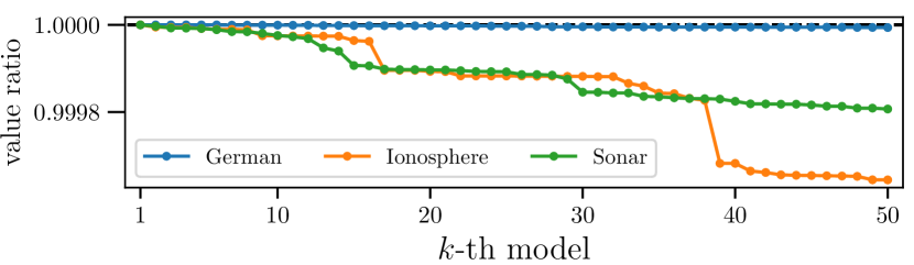
We first evaluated EnumSV on three real datasets, German ($n=1000,d=20$), Ionosphere ($n=351,d=34$), and Sonar ($n=208,d=60$) from UCI ML repository Dheeru & Karra Taniskidou (2017). Their task is a binary classification. We randomly split each dataset into train ($70\%$) and test ($30\%$) samples, and evaluated the test loss by the hinge loss $l(y,{\hat{y}})=\max(0,1-y\cdot{\hat{y}})$. For each dataset, the hyperparameter $C$ was selected by $5$-fold cross validation among $10^{-2},10^{-1},\dots,10^{3}$ before enumeration.

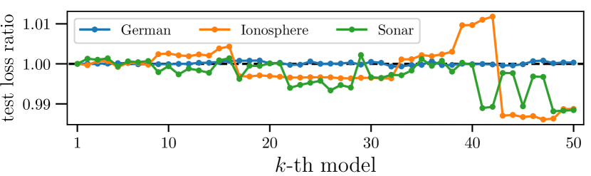
We applied EnumSV to these datasets, and enumerated top-$50$ models. Figure 1 presents the values of the ratio $f(\bm{\alpha}^{(k)})/f(\bm{\alpha}^{(1)})$ of the objective function value and the ratio of the test loss of the $k$-th enumerated model $\bm{\alpha}^{(k)}$ to those of the best model $\bm{\alpha}^{(1)}$. Figure 1 (a) shows that the values of the objective function decreases as the rank $k$ increases as expected from Theorem 1. For German dataset, the objective function values of top-$50$ were almost same within deviation of $6.0\times 10^{-4}$. It indicates that there are multiple models achieving the almost identical objective value. Figure 1 (b) shows that some enumerated model, such as $\bm{\alpha}^{(32)}$ for German, $\bm{\alpha}^{(43)}$ for Ionosphere, and $\bm{\alpha}^{(41)}$ for Sonar, had smaller test loss compared with the optimal model $\bm{\alpha}^{(1)}$. It means that an optimal model is not always the best model, and we obtained a better model with a lower test loss than an optimal model by enumerating models.

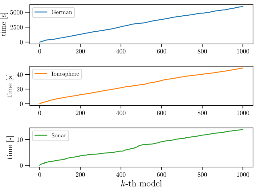
Figure 2 presents the total time of enumerating top-$1000$ models. The total time seems almost linear in rank $k$. Consequently, we conclude that EnumSV has small latency for outputting solutions independent of their ranks, and thus, is scalable in the number $K$ of enumerated models.

5.2 Injected COMPAS Dataset

(a) Demographic parity $\delta(\bm{\alpha}^{(k)}\mid z)$ on the test dataset $S_{\textrm{test}}$.

(b) Misclassification ratio of $\bm{\alpha}^{(k)}$ on $S_{\textrm{test}}$.

Figure 3: Changes of properties of top-50 enumerated models on Injected COMPAS dataset.

Next, we demonstrate an application of EnumSV to a fair classification scenario under false data injection attacks. To evaluate the fairness of the model $m$ for the sensitive attribute $z\in\{-1,1\}$, we used demographic parity (DP) Calders et al. (2009) defined by

$$\delta(m\!\mid\!z):=|P(m(x)\!=\!1\!\mid\!z\!=\!1)-P(m(x)\!=\!1\!\mid\!z\!=\!-1)|,$$

where $P$ is a probability on the joint distribution over $(z,m(x))$. We note that the larger the DP, the larger the discrimination of prediction.

We used COMPAS dataset ($n=6172,d=12$) related to recidivism risk prediction distributed at Adebayo (2018). The task is to predict whether individual people recidivate within two years from their criminal history. We used the attribute ”African_American” as a sensitive attribute $z$. We assume a scenario of false data injection Mo et al. (2010) that is a special kind of attacks to learning algorithms, which increases the DP of the learned model for the sensitive attribute $z$ by flipping output labels $y$ of a small subset of a training dataset. To reproduce this scenario, we generated injected subsets of the COMPAS by the following steps:

1. Create a training dataset $S$ by randomly sampling a subset of the COMPAS with $100$ examples.

2. Randomly choose a subset of $S$ such that $y\not=z$ with $10$ examples, and replace these outputs $y$ by $-y$.

3. Create a test dataset $S_{\textrm{test}}$ by randomly sampling from the COMPAS with $50$ examples.

By our preliminary experiments, we confirm that the above procedure increases the DP of SVM models on $S_{\textrm{test}}$.

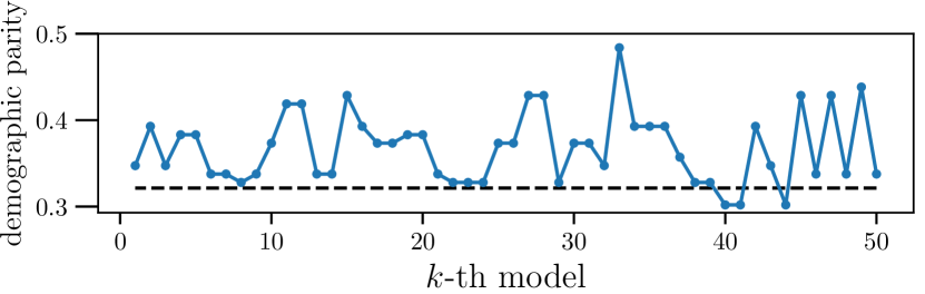
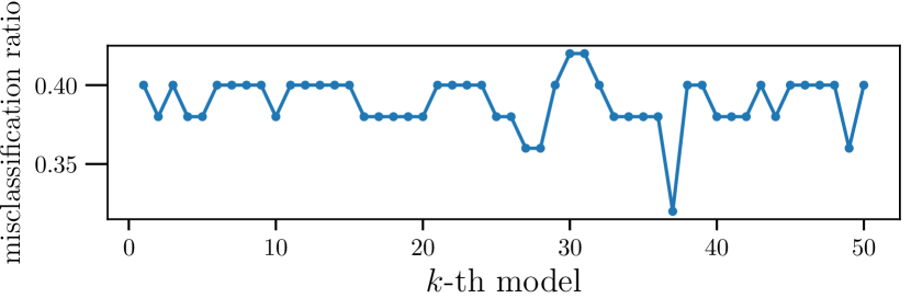
We applied EnumSV to the above injected COMPAS dataset, and measured objective function values, demographic parity (DP), and misclassification ratio of the top-50 enumerated models. We observed that all the enumerated top-$K$ models had the same objective value. However, these prediction results were mutually different.

Figure 2 (a) presents the value of the DP of the enumerated models, where the dashed line indicates the reference DP value $\theta_{*}=0.321$ of the model learned by the non-injected subset of the input $S$. Figure 2 (b) presents the misclassification ratio of the enumerated models $\bm{\alpha}^{(k)}$ on $S_{\textrm{test}}$. From the figures, we observed that EnumSV found the three fair models $\bm{\alpha}^{(40)}$, $\bm{\alpha}^{(41)}$, and $\bm{\alpha}^{(44)}$ achieving lower DP than $\theta_{*}$ and lower misclassification ratio than $\bm{\alpha}^{(1)}$. Consequently, EnumSV successfully obtained several fair models against false data injection by enumerating models.

6 Conclusion

In this paper, we proposed an efficient algorithm to enumerate top-$K$ SVM models with distinct support vectors in descending order of these objective function values. By experiments on real datasets, we demonstrated that our framework provides better models than one single optimal solution, and fair models against false data injection, which increases the unfairness of an optimal model. As future work, we will try to make theoretical or empirical justification of Assumption 1 for a particular class of SVM learning algorithms such as chunking Vapnik (1998) and SMO Platt (1999). It is also interesting future work to extend our algorithm to enumerate models taking their diversity into account so as to interactively help users to understand a dataset.

References

- Adebayo (2018) Adebayo, J. FairML: Auditing black-box predictive models. https://github.com/adebayoj/fairml, 2018.
- Angelino et al. (2017) Angelino, E., Larus-Stone, N., Alabi, D., Seltzer, M., and Rudin, C. Learning certifiably optimal rule lists. In Proc. ACM KDD 2017, Halifax, August, pp. 35–44, 2017.
- Avis & Fukuda (1996) Avis, D. and Fukuda, K. Reverse search for enumeration. Discrete Applied Mathematics, 65(1-3):21–46, 1996.
- Bien & Tibshirani (2011) Bien, J. and Tibshirani, R. Prototype selection for interpretable classification. The Annals of Applied Statistics, 5(4):2403–2424, 2011.
- Burges & Crisp (2000) Burges, C. J. and Crisp, D. J. Uniqueness of the svm solution. In NIPS 1999, pp. 223–229, 2000.
- Calders et al. (2009) Calders, T., Kamiran, F., and Pechenizkiy, M. Building classifiers with independency constraints. In IEEE ICDM 2009 Workshops, pp. 13–18, Dec 2009.
- Cormen et al. (2009) Cormen, T. H., Leiserson, C. E., Rivest, R. L., and Stein, C. Introduction to Algorithms, Third Edition. The MIT Press, 3rd edition, 2009.
- Crawford (2017) Crawford, K. The trouble with bias. NIPS 2017, invited talk, Long Beach, USA, 2017.
- Cristianini & Shawe-Taylor (2000) Cristianini, N. and Shawe-Taylor, J. An Introduction to Support Vector Machines and Other Kernel-based Learning Methods. Cambridge University Press, 2000.
- Dheeru & Karra Taniskidou (2017) Dheeru, D. and Karra Taniskidou, E. UCI machine learning repository, 2017. URL http://archive.ics.uci.edu/ml.
- Hajian et al. (2016) Hajian, S., Bonchi, F., and Castillo, C. Algorithmic bias: From discrimination discovery to fairness-aware data mining. In Proc. ACM KDD 2016, San Francisco, pp. 2125–2126, 2016.
- Hara & Ishihata (2018) Hara, S. and Ishihata, M. Approximate and exact enumeration of rule models. In Proc. AAAI 2018, New Orleans, USA., pp. 3157–3164, 2018.
- Hara & Maehara (2017) Hara, S. and Maehara, T. Enumerate lasso solutions for feature selection. In Proc. AAAI 2017, San Francisco, USA., pp. 1985–1991, 2017.
- Hastie et al. (2001) Hastie, T., Tibshirani, R., and Friedman, J. The Elements of Statistical Learning. Springer Series in Statistics. Springer New York Inc., 2001.
- Hastie et al. (2004) Hastie, T., Rosset, S., Tibshirani, R., and Zhu, J. The entire regularization path for the support vector machine. J. Mach. Learn. Res., 5:1391–1415, December 2004.
- Kim et al. (2016) Kim, B., Khanna, R., and Koyejo, O. Examples are not enough, learn to criticize! criticism for interpretability. In NIPS 2016, Barcelona, pp. 2280–2288. 2016.
- Lawler (1972) Lawler, E. A procedure for computing the k best solutions to discrete optimization problems and its application to the shortest path problem. Manag. Sci., 18(7):401–405, 1972.
- Mo et al. (2010) Mo, Y., Garone, E., Casavola, A., and Sinopoli, B. False data injection attacks against state estimation in wireless sensor networks. In 49th IEEE Conference on Decision and Control (CDC), pp. 5967–5972, Dec 2010.
- Platt (1999) Platt, J. C. Fast training of support vector machines using sequential minimal optimization. In Advances in Kernel Methods, chapter 12, pp. 185–208. MIT Press, 1999.
- Ribeiro et al. (2016) Ribeiro, M. T., Singh, S., and Guestrin, C. ”why should I trust you?”: Explaining the predictions of any classifier. In Proc. ACM KDD 2016, San Francisco, pp. 1135–1144, 2016.
- Ross et al. (2018) Ross, A., Pan, W., and Doshi-Velez, F. Learning qualitatively diverse and interpretable rules for classification. In 2018 ICML Workshop on Human Interpretability in Machine Learning (WHI 2018), 2018. URL https://arxiv.org/abs/1806.08716.
- Ruggieri (2017) Ruggieri, S. Enumerating distinct decision trees. In Proc. ICML 2017, Sydney, pp. 2960–2968, 2017.
- Vapnik (1998) Vapnik, V. N. Statistical Learning Theory. Wiley-Interscience, 1998.