A two-dimensional electrostatic model of interdigitated comb drive in longitudinal mode

Abstract

A periodic homogenization model of the electrostatic equation is constructed for a comb drive with a large number of fingers and whose mode of operation is in-plane and longitudinal. The model is obtained in the case where the distance between the rotor and the stator is of an order $\varepsilon^{\alpha}$, $\alpha\geq 2$, where $\varepsilon$ denotes the period of distribution of the fingers. The model derivation uses the two-scale convergence technique. Strong convergences are also established. This allows us to find, after a proper scaling, the limit of the electrostatic force applied to the rotor in the longitudinal direction.

Keywords: Comb drive, electrostatic forces, MEMS, homogenization

2010 AMS subject classifications: 35J05, 35B27

1 Introduction

The technology of Micro-Electro-Mechanical Systems, or MEMS, includes both mechanical and electronic components on a single chip built with micro fabrication techniques. The main MEMS parts are sensors, actuators, and microelectronics. Many types of micro actuation techniques are available, the most common of which are piezoelectric, magnetic, thermal, electrochemical, and electrostatic actuation. The latter is clearly the most widespread because of its compatibility with microfabrication technology, its ease of integration and its low energy consumption. In particular, electrostatic comb drives, introduced in [52, 51] to enable large travel range at low driving voltage, are among the most used electrostatically actuated devices in microelectromechanical systems containing movable mechanical structures.

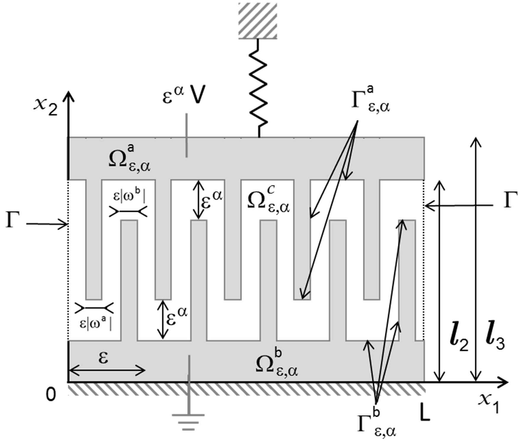
Figure 1: The comb drive

A comb drive is a deformable capacitor consisting of conductive stator and rotor, each one composed of parallel fingers, that are interdigitated, and whose number may exceed one hundred. The stator is clamped and the rotor is suspended on elastic springs. The elastic suspension is designed to allow the rotor to move in one of the desired directions: longitudinal direction, i.e. parallel to the fingers, or in one of the two perpendicular directions. From the electrical point of view, the stator is grounded and the rotor is subjected to an electric potential $V$. The difference in voltage induces an electrostatic force between the stator and the rotor which causes a displacement of the rotor and therefore restoring forces in the suspension. The equilibrium state is reached when the mechanical restoring forces balance the electrostatic force.

The advantages of using electrostatic comb drive actuator approach include low power dissipation, simple electronic control, and easy capacity-based sensing mechanism. These devices are intended for applications in mechanical sensors, RF communication, microbiology, mechanical power transmission, long-range actuation, microphotonics, and microfluids [51, 55, 38, 33].

To achieve considerable electrostatic forces without reverting to excessively high driving voltages, the freespace gap between the electrodes must be minimal. With the advances of microfabrication technology, thinner fingers and smaller gaps can be micromachined. This can allow for a denser spacing of fingers and thus increase the power density of comb drive actuators.

Design of complex MEMS involving multiple comb drives can not be performed by trial and error due to the high microfabrication cost and time consumption. Designers then make an intensive use of models. Part of the comb drive modeling works focuse on the development of analytical models that, beyond taking into account the electrostatic forces between parallel parts, describe the fringe fields according to different methods and in many configurations [37], [54], [34], [35] [43], [36], [43], and the analytical models in the software package Coventor MEMS+ [20]. On the other side, the use of direct numerical simulation remains the reference approach for general configurations. Most often it is carried out by a finite element method [25], [16], [50], or a boundary element method [17], [44]. Despite the impressive increase of computer power, the time scale required by their use for direct simulation, optimization or calibration of complex systems is still incompatible with the time scale of a designer.

Until now, the use of multiscale methods has not been yet explored on this family of problems despite their periodic structure. However, they can offer a good compromise between numerical methods adapted to general physics and geometries, but expensive in simulation time, and analytical methods developed for particular physics and geometries requiring only a few computation resources.

In this paper we develop a first comb drive multiscale model based on asymptotic methods. Precisely, we consider a 2-dimensional model for an in-plane comb drive, in a vacuum and in statical longitudinal regime, made by a rotor called $\Omega^{a}_{\varepsilon,\alpha}$ and a stator called $\Omega^{b}_{\varepsilon,\alpha}$ (see Figure 1). Both of them are composed by a set of $\varepsilon$-periodic fingers, with cross-section of order $\varepsilon$. The goal of this paper is to study the asymptotic behaviour of the longitudinal electrostatic force applied on the rotor with respect to two parameters: the period $\varepsilon$ and the small distance between the rotor and the stator. A priori estimates show that in this model a discriminating role is played by this distance that we consider of order $\varepsilon^{\alpha}$. Precisely, we prove that if $\alpha\geq 2$ for obtaining asymptotically a force of order $O(1)$, the applied voltage has to be of order $\varepsilon^{\alpha}V$ and in this case the limit force is given by

$$-\frac{\epsilon_{0}}{2}V^{2}L\left(\hbox{meas}(\omega^{a})+\hbox{meas}(\omega^{b})\right)$$ (1.1)

where $\epsilon_{0}$ is the vacuum permittivity, $V$ is a constant independent of $\varepsilon$, $L$ the comb length, and $\hbox{meas}(\omega^{a})$ and $\hbox{meas}(\omega^{b})$ the length of the cross section of the reference finger of the rotor and of the stator, respectively (see Figure 1). This result shows that only the longitudinal forces on the extremities of the rotor’s fingers and on the part of the rotor’s boundary corresponding to the orthogonal projection of the stator’s fingers play a significant role. In particular, this means that the fringe field can be neglected in the asymptotic regime $\alpha\geq 2$. We expect that this phenomenon appears when $0\leq\alpha<2$. We also underline that in the limit force there is no contribution of boundary layer effect on the lateral side of the comb, that are expected in other regimes.

The paper is organized in the following way. The geometry of the comb drive is rigorously described in Section 2. The problem satisfied by the electrical potential in the vacuum between the rotor and the stator is given in Section 3 (see (3.1) where the voltage source is normalized by assuming it equal to 1). The main result of this paper, i.e. the proof of formula (1.1), is stated in Theorem 3.1. Section 4 is devoted to rescale the problem given in Section 3 to a problem on a domain where the finger’s height is independent of $\varepsilon$ (see Figure 3). Thus, the problem is split on three subdomains $\Omega^{c,1}_{\varepsilon}$, $\Omega^{c,2}_{\varepsilon}$, and $\Omega^{c,3}_{\varepsilon}$ (see Figure 3). Moreover, in Proposition 4.1 we prove a key result which allows us to transform the longitudinal force applied on the rotor’s boundary part $\Gamma^{a}_{\varepsilon,\alpha}$ (see formula in (3.3) and also p. 225 in [39]) into an integral on $\Omega^{c,1}_{\varepsilon}\cup\Omega^{c,2}_{\varepsilon}\cup\Omega^{c,3}_{\varepsilon}$. A priori estimates of the rescaled solution of problem (3.1) are obtained in Section 5. They suggest that different regimes depending on $\alpha$ can be expected. Section 6 is devoted to prove Theorem 3.1 in the case $\alpha=2$. The proof consists of several steps. In Section 6.1, further a priori estimates of the rescaled solution are derived in the case $\alpha=2$. These estimates provide two-scale convergences (the two-scale convergence technique was proposed in [49] and developed in [2], see also [14], [19], and [40]). Then, in Section 6.2 the two-scale limits are identified on each subdomain $\Omega^{c,1}$, $\Omega^{c,2}$, and $\Omega^{c,3}$ (see Figure 4). The limit results are improved in Section 6.3 by corrector results. Finally in Section 6.4, these correctors allow us to pass to the limit in the formula of the longitudinal force stated in Proposition 4.1 and to prove Theorem 3.1 in the case $\alpha=2$. The proof of Theorem 3.1 in the case $\alpha>2$ is only sketched in Section 7.

Homogenization of oscillating boundaries with fixed amplitude is widely studied and we refer to the following main papers: [1], [3], [4], [5], [6], [7], [8], [9], [10], [11], [12], [13], [15], [21], [22], [23], [24], [26], [27], [28], [29], [30], [31], [32], [41] [42], [45], [46], [47], [48], and [53].

Also the homogenization of boundaries with oscillations having small amplitude has a wide bibliography, but this argument is beyond the scope of this paper and a reader interested in this subject can see some references quoted in [30].

2 The geometry

Let $\zeta_{1},\,\zeta_{2},\,\zeta_{3},\,\zeta_{4}\in]0,1[$ be such that

$$\zeta_{1}<\zeta_{2}<\zeta_{3}<\zeta_{4},$$

and set

$$\omega^{a}=]\zeta_{1},\zeta_{2}[,\quad\omega^{b}=]\zeta_{3},\zeta_{4}[,$$

$$\hbox{meas}(\omega^{a})=\zeta_{2}-\zeta_{1},\quad\hbox{meas}(\omega^{b})=\zeta_{4}-\zeta_{3}.$$

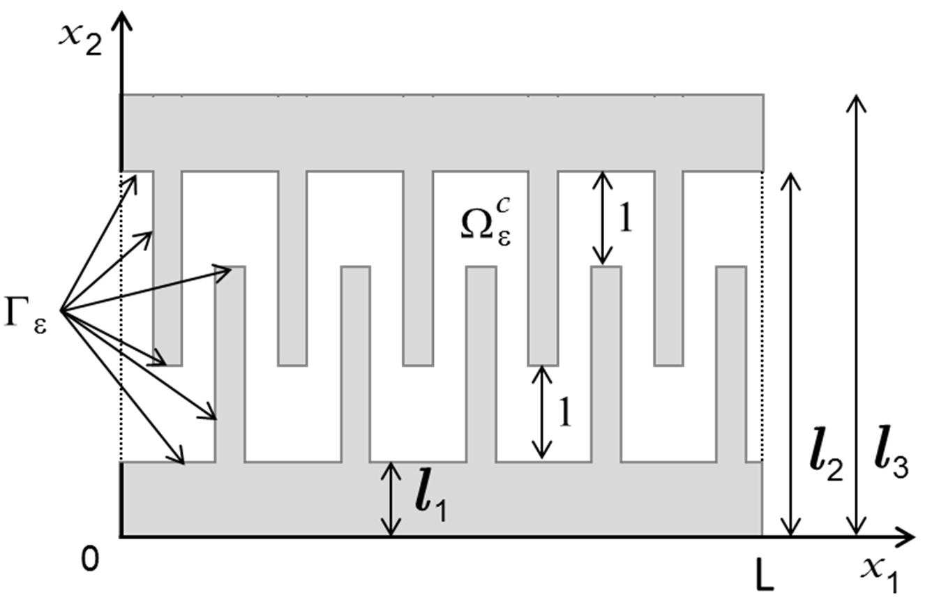
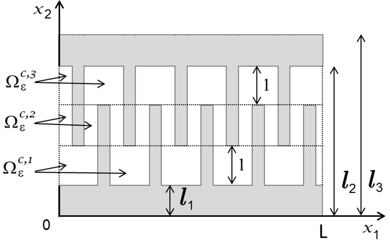
Figure 2: The rescaled comb drive

Figure 3: Decomposition of the rescaled comb drive

Let $\alpha\in[0,+\infty[$, $L\in]0,+\infty[$, and $l_{1},l_{2},l_{3}\in]0,+\infty[$ be such that

$$l_{1}+2<l_{2}<l_{3}.$$

For every $\varepsilon\in\left\{\frac{L}{n}:n\in\mathbb{N}\right\}$ set (see Figure 1 for $\alpha>0$ or Figure 3 for $\alpha=0$)

$$\Omega^{a}_{\varepsilon,\alpha}=\left(]0,L[\times]l_{2},l_{3}[\right)\cup\left(\bigcup_{k=0}^{\frac{L}{\varepsilon}-1}\left(\varepsilon\omega^{a}+\varepsilon k\right)\times]l_{1}+\varepsilon^{\alpha},l_{2}]\right),$$

$$\Omega^{b}_{\varepsilon,\alpha}=\left(]0,L[\times]0,l_{1}[\right)\cup\left(\bigcup_{k=0}^{\frac{L}{\varepsilon}-1}\left(\varepsilon\omega^{b}+\varepsilon k\right)\times[l_{1},l_{2}-\varepsilon^{\alpha}[\right),$$

$$\Omega^{c}_{\varepsilon,\alpha}=\left(]0,L[\times]0,l_{3}[\right)\setminus\left(\overline{\Omega^{a}_{\varepsilon,\alpha}}\cup\overline{\Omega^{b}_{\varepsilon,\alpha}}\right),$$

$$\Gamma^{a}_{\varepsilon,\alpha}=\partial\Omega^{a}_{\varepsilon,\alpha}\cap\partial\Omega^{c}_{\varepsilon,\alpha},$$

$$\Gamma^{b}_{\varepsilon,\alpha}=\partial\Omega^{b}_{\varepsilon,\alpha}\cap\partial\Omega^{c}_{\varepsilon,\alpha},$$

$$\Gamma_{\varepsilon,\alpha}=\Gamma^{a}_{\varepsilon,\alpha}\cup\Gamma^{b}_{\varepsilon,\alpha},$$

$$\Gamma=\{0,L\}\times]l_{1},l_{2}[.$$

where $\Omega^{a}_{\varepsilon,\alpha}$ models the rotor, $\Omega^{b}_{\varepsilon,\alpha}$ the stator, each one composed of parallel fingers that are interdigitated, $\Omega^{c}_{\varepsilon,\alpha}$ the vacuum between the rotor and the stator, and $\Gamma^{a}_{\varepsilon,\alpha}$ and $\Gamma^{b}_{\varepsilon,\alpha}$ are the parts of the boundary of the rotor and of the stator facing each other. Moreover, setting (see Figure 3 for $\alpha=0$)

$$\Omega^{c,1}_{\varepsilon,\alpha}=\Omega^{c}_{\varepsilon,\alpha}\cap\left(]0,L[\times]l_{1},l_{1}+\varepsilon^{\alpha}[\right),$$

$$\Omega^{c,2}_{\varepsilon,\alpha}=\Omega^{c}_{\varepsilon,\alpha}\cap\left(]0,L[\times[l_{1}+\varepsilon^{\alpha},l_{2}-\varepsilon^{\alpha}]\right),$$

$$\Omega^{c,3}_{\varepsilon,\alpha}=\Omega^{c}_{\varepsilon,\alpha}\cap\left(]0,L[\times]l_{2}-\varepsilon^{\alpha},l_{2}[\right),$$

the vacuum is split in three parts

$$\Omega^{c}_{\varepsilon,\alpha}=\Omega^{c,1}_{\varepsilon,\alpha}\cup\Omega^{c,2}_{\varepsilon,\alpha}\cup\Omega^{c,3}_{\varepsilon,\alpha}.$$

Furthermore, set (see Figure 4)

$$\Omega^{c,1}=]0,L[\times]l_{1},l_{1}+1[,\quad\Omega^{c,2}=]0,L[\times]l_{1}+1,l_{2}-1[,\quad\Omega^{c,3}=]0,L[\times]l_{2}-1,l_{2}[.$$

Remark 2.1.

For simplicity we assumed $\varepsilon\in\left\{\frac{L}{n}:n\in\mathbb{N}\right\}$. Of course, with small modifications in the proofs, all results of this paper hold true with $\varepsilon\in]0,1[$.

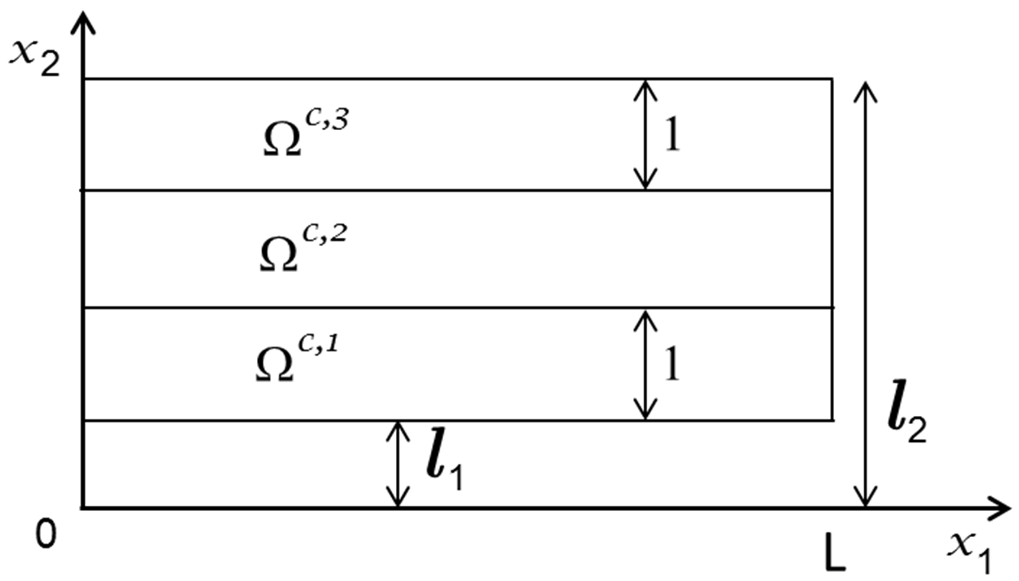
Figure 4: The limit domains

3 The problem

Let $\alpha\in[0,+\infty[$. Then, for every $\varepsilon$ consider the following normalized problem

$$\left\{\begin{array}[]{lll}-\Delta\phi_{\varepsilon}=0,\hbox{ in }\Omega^{c}_{\varepsilon,\alpha},\\ \\ \phi_{\varepsilon}=1,\hbox{ on }\Gamma^{a}_{\varepsilon,\alpha},\\ \\ \phi_{\varepsilon}=0,\hbox{ on }\Gamma^{b}_{\varepsilon,\alpha},\\ \\ \nabla\phi_{\varepsilon}\cdot\nu=0,\hbox{ on }\Gamma,\end{array}\right.$$ (3.1)

where $\nu$ denotes the unit normal to $\Gamma$ exterior to $\Omega^{c}_{\varepsilon,\alpha}$. The solution $\phi_{\varepsilon}$ represents the electrical potential in the vacuum $\Omega^{c}_{\varepsilon,\alpha}$ when the stator is grounded and the voltage in the rotor is assumed equal to $1$. By setting

$$\mu_{\varepsilon,\alpha}=\left\{\begin{array}[]{ll}1,\hbox{ on }\Gamma^{a}_{\varepsilon,\alpha},\\ \\ 0,\hbox{ on }\Gamma^{b}_{\varepsilon,\alpha},\end{array}\right.$$

the weak formulation of (3.1) is

$$\left\{\begin{array}[]{lll}\phi_{\varepsilon}\in H^{1}_{\Gamma_{\varepsilon,\alpha}}(\Omega^{c}_{\varepsilon,\alpha},\mu_{\varepsilon,\alpha}),\\ \\ \displaystyle{\int_{\Omega^{c}_{\varepsilon,\alpha}}\nabla\phi_{\varepsilon}\nabla\psi dx=0,\quad\forall\psi\in H^{1}_{\Gamma_{\varepsilon,\alpha}}(\Omega^{c}_{\varepsilon,\alpha},0),}\end{array}\right.$$ (3.2)

where for $g\in H^{-\frac{1}{2}}(\Gamma_{\varepsilon,\alpha})$ it is set

$$H^{1}_{\Gamma_{\varepsilon,\alpha}}(\Omega^{c}_{\varepsilon,\alpha},g)=\{\psi\in H^{1}(\Omega^{c}_{\varepsilon,\alpha}):\psi=g,\hbox{ on }\Gamma_{\varepsilon,\alpha}\}.$$

According to [39], p. 225, the longitudinal electrostatic force on rotor’s boundary $\Gamma^{a}_{\varepsilon,\alpha}$ generated by the electrical potential $\varepsilon^{\alpha}V\phi_{\varepsilon}$ in the vacuum is given by

$$-\frac{\epsilon_{0}}{2}V^{2}\int_{\Gamma^{a}_{\varepsilon,\alpha}}|\varepsilon^{\alpha}\nabla\phi_{\varepsilon}|^{2}\nu_{2}\,ds,$$ (3.3)

where $\epsilon_{0}$ is the vacuum permittivity,$V$ is a constant independent of $\varepsilon$, and $\nu_{2}$ denotes the second component of the unit normal to $\Gamma^{a}_{\varepsilon,\alpha}$ exterior to $\Omega^{c}_{\varepsilon,\alpha}$.

The main result of this paper is the following one.

Theorem 3.1.

For every $\varepsilon$, let $\phi_{\varepsilon}$ be the unique solution to (3.2) with $\alpha\geq 2$ and let $\nu_{2}$ denote the second component of the unit normal to $\Gamma^{a}_{\varepsilon,\alpha}$ exterior to $\Omega^{c}_{\varepsilon,\alpha}$. Then,

$$\lim_{\varepsilon\rightarrow 0}\int_{\Gamma^{a}_{\varepsilon,\alpha}}|\varepsilon^{\alpha}\nabla\phi_{\varepsilon}|^{2}\nu_{2}\,ds=L\left(\hbox{meas}(\omega^{a})+\hbox{meas}(\omega^{b})\right),$$ (3.4)

where $L$, $\omega^{a}$, and $\omega^{b}$ are defined in Section 2.

In the sequel, the dependence on $\alpha$ of the domain will be omitted when $\alpha=0$. For instance, $\Omega^{a}_{\varepsilon,0}$ will be denoted by $\Omega^{a}_{\varepsilon}$, and so on.

4 The rescaling

By virtue of transformation (see Figure 1 and Figure 3)

$$T_{\varepsilon,\alpha}:\Omega^{c}_{\varepsilon}\rightarrow\Omega^{c}_{\varepsilon,\alpha}$$ (4.1)

defined by

$$\left\{\begin{array}[]{ll}(x_{1},x_{2})\in\Omega^{c,1}_{\varepsilon}\rightarrow\left(x_{1},(x_{2}-l_{1})\varepsilon^{\alpha}+l_{1}\right)\in\Omega^{c,1}_{\varepsilon,\alpha},\\ \\ (x_{1},x_{2})\in\Omega^{c,2}_{\varepsilon}\rightarrow\left(x_{1},D_{\varepsilon}(x_{2}-l_{1}-1)+l_{1}+\varepsilon^{\alpha}\right)\in\Omega^{c,2}_{\varepsilon,\alpha},\\ \\ (x_{1},x_{2})\in\Omega^{c,3}_{\varepsilon}\rightarrow\left(x_{1},(x_{2}-l_{2}+1)\varepsilon^{\alpha}+l_{2}-\varepsilon^{\alpha}\right)\in\Omega^{c,3}_{\varepsilon,\alpha},\end{array}\right.$$ (4.2)

with

$$D_{\varepsilon}=\frac{l_{2}-l_{1}-2\varepsilon^{\alpha}}{l_{2}-l_{1}-2},$$ (4.3)

problem (3.2) is rescaled in the following one

$$\left\{\begin{array}[]{lll}\varphi_{\varepsilon}\in H^{1}_{\Gamma_{\varepsilon}}(\Omega^{c}_{\varepsilon},\mu_{\varepsilon}),\\ \\ \displaystyle{\int_{\Omega^{c,1}_{\varepsilon}\cup\Omega^{c,3}_{\varepsilon}}\left(\varepsilon^{\alpha}\partial_{x_{1}}\varphi_{\varepsilon}\partial_{x_{1}}\psi+\varepsilon^{-\alpha}\partial_{x_{2}}\varphi_{\varepsilon}\partial_{x_{2}}\psi\right)dx}\\ \\ \displaystyle{+\int_{\Omega^{c,2}_{\varepsilon}}\left(D_{\varepsilon}\partial_{x_{1}}\varphi_{\varepsilon}\partial_{x_{1}}\psi+D^{-1}_{\varepsilon}\partial_{x_{2}}\varphi_{\varepsilon}\partial_{x_{2}}\psi\right)dx=0,\quad\forall\psi\in H^{1}_{\Gamma_{\varepsilon}}(\Omega^{c}_{\varepsilon},0).}\end{array}\right.$$ (4.4)

Remark that

$$\lim_{\varepsilon\rightarrow 0}D_{\varepsilon}=\frac{l_{2}-l_{1}}{l_{2}-l_{1}-2}.$$ (4.5)

Let

$$\varphi^{\star}\in C^{\infty}(\mathbb{R}\times[l_{1},l_{2}])$$ (4.6)

be such that

$$\left\{\begin{array}[]{ll}\varphi^{\star}(\cdot,x_{2})\hbox{ is 1-periodic for every }x_{2}\in[l_{1},l_{2}],\\ \\ \varphi^{\star}=1,\hbox{ in }\omega^{a}\times]l_{1}+1,l_{2}[,\quad\varphi^{\star}=0,\hbox{ in }\omega^{b}\times]l_{1},l_{2}-1[,\\ \\ \varphi^{\star}=1,\hbox{ on }\mathbb{R}\times\{l_{2}\},\quad\varphi^{\star}=0,\hbox{ on }\mathbb{R}\times\{l_{1}\},\end{array}\right.$$ (4.7)

and for every $\varepsilon\in]0,1[$ set

$$\varphi^{\star}_{\varepsilon}(x_{1},x_{2})=\varphi^{\star}\left(\frac{x_{1}}{\varepsilon},x_{2}\right),\hbox{ in }\mathbb{R}\times[l_{1},l_{2}].$$ (4.8)

The previous rescaling allows us to rewrite formula (3.3).

Proposition 4.1.

For every $\varepsilon$, let $\phi_{\varepsilon}$ be the unique solution to (3.2), $\varphi_{\varepsilon}$ be the unique solution to (4.4), $\varphi^{\star}_{\varepsilon}$ be defined by (4.6)-(4.8), $D_{\varepsilon}$ be defined in (4.3), and let $\nu_{2}$ denote the second component of the unit normal to $\Gamma^{a}_{\varepsilon,\alpha}$ exterior to $\Omega^{c}_{\varepsilon,\alpha}$. Then, for every $\varepsilon$,

$$\begin{array}[]{ll}\displaystyle{\int_{\Gamma^{a}_{\varepsilon,\alpha}}|\nabla\phi_{\varepsilon}|^{2}\nu_{2}ds=}\\ \\ \displaystyle{\int_{\Omega^{c,1}_{\varepsilon}\cup\Omega^{c,3}_{\varepsilon}}\left(-\partial_{x_{2}}\varphi^{\star}_{\varepsilon}\left(\left|\partial_{x_{1}}\varphi_{\varepsilon}\right|^{2}-\frac{1}{\varepsilon^{2\alpha}}\left|\partial_{x_{2}}\varphi_{\varepsilon}\right|^{2}\right)+2\partial_{x_{2}}\varphi_{\varepsilon}\partial_{x_{1}}\varphi^{\star}_{\varepsilon}\partial_{x_{1}}\varphi_{\varepsilon}\right)dx}\\ \\ \displaystyle{+\int_{\Omega^{c,2}_{\varepsilon}}\left(-\partial_{x_{2}}\varphi^{\star}_{\varepsilon}\left(\left|\partial_{x_{1}}\varphi_{\varepsilon}\right|^{2}-\frac{1}{D_{\varepsilon}^{2}}\left|\partial_{x_{2}}\varphi_{\varepsilon}\right|^{2}\right)+2\partial_{x_{2}}\varphi_{\varepsilon}\partial_{x_{1}}\varphi^{\star}_{\varepsilon}\partial_{x_{1}}\varphi_{\varepsilon}\right)dx.}\end{array}$$ (4.9)

Proof.

Let $T_{\varepsilon,\alpha}$ be defined by (4.1)-(4.3). The first step is devoted to proving that

$$\begin{array}[]{lll}\displaystyle{\int_{\Gamma^{a}_{\varepsilon,\alpha}}|\nabla\phi_{\varepsilon}|^{2}\nu_{2}ds}\\ \\ \displaystyle{=\int_{\Omega_{\varepsilon,\alpha}^{c}}\left(-\partial_{x_{2}}\left(\varphi^{\star}_{\varepsilon}\circ T_{\varepsilon,\alpha}^{-1}\right)\left|\nabla\phi_{\varepsilon}\right|^{2}+2\partial_{x_{2}}\phi_{\varepsilon}\nabla\left(\varphi^{\star}_{\varepsilon}\circ T_{\varepsilon,\alpha}^{-1}\right)\nabla\phi_{\varepsilon}\right)dx,\quad\forall\varepsilon,}\end{array}$$ (4.10)

from which (4.10) follows by changing of variable (4.1) in the second integral.

As we shall show in the following,

$$|\nabla\phi_{\varepsilon}|^{2}\in W^{1,1}(\Omega_{\varepsilon,\alpha}^{c}).$$ (4.11)

In particular, also $(\varphi_{\varepsilon}^{\star}\circ T_{\varepsilon,\alpha}^{-1})|\nabla\phi_{\varepsilon}|^{2}$ belongs to $W^{1,1}(\Omega_{\varepsilon,\alpha}^{c})$. Thus, definitions (4.1) and (4.6)-(4.8) allow us to write

$$\begin{array}[]{ll}\displaystyle{\int_{\Gamma_{\varepsilon,\alpha}^{a}}|\nabla\phi_{\varepsilon}|^{2}\nu_{2}ds=\int_{\Gamma_{\varepsilon,\alpha}^{a}}(\varphi_{\varepsilon}^{\star}\circ T_{\varepsilon,\alpha}^{-1})|\nabla\phi_{\varepsilon}|^{2}\nu_{2}ds}\\ \\ \displaystyle{=\int_{\Gamma_{\varepsilon,\alpha}\cup\Gamma}(\varphi_{\varepsilon}^{\star}\circ T_{\varepsilon,\alpha}^{-1})|\nabla\phi_{\varepsilon}|^{2}\nu_{2}ds,\quad\forall\varepsilon.}\end{array}$$ (4.12)

The Green’s Formula (for instance, see Th. 6.6-7 in [18]) gives

$$\int_{\Gamma_{\varepsilon,\alpha}\cup\Gamma}(\varphi_{\varepsilon}^{\star}\circ T_{\varepsilon,\alpha}^{-1})|\nabla\phi_{\varepsilon}|^{2}\nu_{2}ds=\int_{\Omega_{\varepsilon,\alpha}^{c}}\partial_{x_{2}}((\varphi_{\varepsilon}^{\star}\circ T_{\varepsilon,\alpha}^{-1})|\nabla\phi_{\varepsilon}|^{2})dx,\quad\forall\varepsilon.$$ (4.13)

Then, (4.12) and (4.13)) provides

$$\begin{array}[]{ll}\displaystyle{\int_{\Gamma_{\varepsilon,\alpha}^{a}}|\nabla\phi_{\varepsilon}|^{2}\nu_{2}ds}\\ \\ \displaystyle{=\int_{\Omega_{\varepsilon,\alpha}^{c}}\partial_{x_{2}}(\varphi_{\varepsilon}^{\star}\circ T_{\varepsilon,\alpha}^{-1})|\nabla\phi_{\varepsilon}|^{2}dx+2\int_{\Omega_{\varepsilon,\alpha}^{c}}(\varphi_{\varepsilon}^{\star}\circ T_{\varepsilon,\alpha}^{-1})\nabla\phi_{\varepsilon}\nabla(\partial_{x_{2}}\phi_{\varepsilon})dx,\quad\forall\varepsilon.}\end{array}$$ (4.14)

On the other side (see below),

$$\nabla\phi_{\varepsilon}\in W^{1,\frac{3}{2}}(\Omega_{\varepsilon,\alpha}^{c}).$$ (4.15)

In particular, $(\varphi_{\varepsilon}^{\star}\circ T_{\varepsilon,\alpha}^{-1})\nabla\phi_{\varepsilon}$ belongs to $W^{1,\frac{3}{2}}(\Omega_{\varepsilon,\alpha}^{c})$, and $\partial_{x_{2}}\phi_{\varepsilon}$ belongs to $W^{1,\frac{3}{2}}(\Omega_{\varepsilon,\alpha}^{c})$ which is included in $W^{1,\frac{6}{5}}(\Omega_{\varepsilon,\alpha}^{c})$. Consequently, again applying the Green’s Formula as it appears in Theorem 6.6-7 in [18] with exponents $p=\frac{3}{2}$ and $q=\frac{6}{5}$, the last integral in the right-hand side of (4.14) becomes

$$\begin{array}[]{ll}\displaystyle{\int_{\Omega_{\varepsilon,\alpha}^{c}}(\varphi_{\varepsilon}^{\star}\circ T_{\varepsilon,\alpha}^{-1})\nabla\phi_{\varepsilon}\nabla(\partial_{x_{2}}\phi_{\varepsilon})dx}\\ \\ \displaystyle{=-\int_{\Omega_{\varepsilon,\alpha}^{c}}{div}((\varphi_{\varepsilon}^{\star}\circ T_{\varepsilon,\alpha}^{-1})\nabla\phi_{\varepsilon})\text{ }\partial_{x_{2}}\phi_{\varepsilon}dx+\int_{\Gamma_{\varepsilon,\alpha}\cup\Gamma}(\varphi_{\varepsilon}^{\star}\circ T_{\varepsilon,\alpha}^{-1})\partial_{x_{2}}\phi_{\varepsilon}\nabla\phi_{\varepsilon}\nu ds,\quad\forall\varepsilon,}\end{array}$$ (4.16)

where $\nu$ is the unit normal to $\Gamma_{\varepsilon,\alpha}\cup\Gamma$ exterior to $\Omega_{\varepsilon,\alpha}^{c}$. Since

$$\int_{\Gamma_{\varepsilon,\alpha}\cup\Gamma}(\varphi_{\varepsilon}^{\star}\circ T_{\varepsilon,\alpha}^{-1})\partial_{x_{2}}\phi_{\varepsilon}\nabla\phi_{\varepsilon}\nu ds=\int_{\Gamma_{\varepsilon,\alpha}^{a}}|\nabla\phi_{\varepsilon}|^{2}\nu_{2}ds,\quad\forall\varepsilon,$$

which can be checked by inspectioning on each part of $\Gamma_{\varepsilon,\alpha}\cup\Gamma$, one can rewrite (4.16) as

$$\begin{array}[]{ll}\displaystyle{\int_{\Omega_{\varepsilon,\alpha}^{c}}(\varphi_{\varepsilon}^{\star}\circ T_{\varepsilon,\alpha}^{-1})\nabla\phi_{\varepsilon}\partial_{x_{2}}\nabla\phi_{\varepsilon}dx}\\ \\ \displaystyle{=-\int_{\Omega_{\varepsilon,\alpha}^{c}}{div}((\varphi_{\varepsilon}^{\star}\circ T_{\varepsilon,\alpha}^{-1})\nabla\phi_{\varepsilon})\text{ }\partial_{x_{2}}\phi_{\varepsilon}dx+\int_{\Gamma_{\varepsilon,\alpha}^{a}}|\nabla\phi_{\varepsilon}|^{2}\nu_{2}ds,\quad\forall\varepsilon.}\end{array}$$ (4.17)

Comparing (4.14) and (4.17) gives

$$\begin{array}[]{ll}\displaystyle{\int_{\Gamma_{\varepsilon,\alpha}^{a}}|\nabla\phi_{\varepsilon}|^{2}\nu_{2}ds}\\ \\ \displaystyle{=-\int_{\Omega_{\varepsilon,\alpha}^{c}}\partial_{x_{2}}(\varphi_{\varepsilon}^{\star}\circ T_{\varepsilon,\alpha}^{-1})|\nabla\phi_{\varepsilon}|^{2}dx+2\int_{\Omega_{\varepsilon,\alpha}^{c}}{div}((\varphi_{\varepsilon}^{\star}\circ T_{\varepsilon,\alpha}^{-1})\nabla\phi_{\varepsilon})\partial_{x_{2}}\phi_{\varepsilon}dx}\\ \\ \displaystyle{=-\int_{\Omega_{\varepsilon,\alpha}^{c}}\partial_{x_{2}}(\varphi_{\varepsilon}^{\star}\circ T_{\varepsilon,\alpha}^{-1})|\nabla\phi_{\varepsilon}|^{2}dx+2\int_{\Omega_{\varepsilon,\alpha}^{c}}\nabla(\varphi_{\varepsilon}^{\star}\circ T_{\varepsilon,\alpha}^{-1})\nabla\phi_{\varepsilon}\partial_{x_{2}}\phi_{\varepsilon}dx}\\ \\ \displaystyle{+\int_{\Omega_{\varepsilon,\alpha}^{c}}(\varphi_{\varepsilon}^{\star}\circ T_{\varepsilon,\alpha}^{-1})\Delta\phi_{\varepsilon}\partial_{x_{2}}\phi_{\varepsilon}dx,\quad\forall\varepsilon,}\end{array}$$

which provides (4.10) since $\Delta\phi_{\varepsilon}=0$ in $\Omega_{\varepsilon,\alpha}^{c}$.

Now, we sketch the proof of (4.11), based on the decomposition of $\phi_{\varepsilon}$ as a sum of its singular and regular parts $\phi_{\varepsilon}^{S}\in H^{1}(\Omega_{\varepsilon,\alpha}^{c})$ and $\phi_{\varepsilon}^{S}\in H^{2}(\Omega_{\varepsilon,\alpha}^{c})$. At the vicinity of any reentering corner with angle $\omega=\frac{3\pi}{2}$, the expression in polar coordinate of the singular part reads

$$\phi_{\varepsilon}^{S}(r,\theta)=r^{\frac{2}{3}}\sin\left(\frac{2\theta}{3}\right).$$

Thus,

$$|\nabla\phi_{\varepsilon}^{S}|^{2}(r,\theta)=r^{-\frac{2}{3}}\Phi_{0}(\theta),$$

with $\Phi_{0}\in C^{\infty}$. The expansion of $\nabla|\nabla\phi_{\varepsilon}|^{2}$ in $\phi_{\varepsilon}^{S}$ and $\phi_{\varepsilon}^{R}$ includes four terms:

$$\nabla|\nabla\phi_{\varepsilon}^{S}|^{2},\quad\nabla\nabla\phi_{\varepsilon}^{S}\nabla\phi_{\varepsilon}^{R},\quad\nabla|\nabla\phi_{\varepsilon}^{R}|^{2},\hbox{ and }\nabla\nabla\phi_{\varepsilon}^{R}\nabla\phi_{\varepsilon}^{S},$$ (4.18)

of which only the first two terms cause regularity problems.

As the first term in (4.18) is concerned, one has

$$\nabla|\nabla\phi_{\varepsilon}^{S}|^{2}(r,\theta)=r^{-\frac{5}{3}}\Phi_{1}(\theta),$$

with $\Phi_{1}\in C^{\infty}$. Then, it is integrable. As the second term in (4.18) is concerned, one has

$$\nabla\nabla\phi_{\varepsilon}^{S}\nabla\phi_{\varepsilon}^{R}=(r^{\frac{1}{3}}\nabla\nabla\phi_{\varepsilon}^{S})(r^{-\frac{1}{3}}\nabla\phi_{\varepsilon}^{R})$$

and its integrability comes from the observation that both terms $r^{\frac{1}{3}}\nabla\nabla\phi_{\varepsilon}^{S}$ are $r^{-\frac{1}{3}}\nabla\phi_{\varepsilon}^{R}$ are square integrable.

The contribution of the corners with mixed conditions, that is at the ends of $\Gamma$, to the singular part is in $H^{2-\eta}(\Omega_{\varepsilon,\alpha}^{c})$ for any positive $\eta$ and does not yield any regularity issue.

Regularity result (4.15) can be proved with the same arguments.

∎

5 A priori estimates

Proposition 5.1.

For every $\varepsilon$, let $\varphi_{\varepsilon}$ be the unique solution to (4.4). Then

$$\exists c\in]0,+\infty[\quad:\quad\left\{\begin{array}[]{lll}\displaystyle{\int_{\Omega^{c,1}_{\varepsilon}\cup\Omega^{c,3}_{\varepsilon}}|\partial_{x_{1}}\varphi_{\varepsilon}|^{2}dx\leq c\left(\varepsilon^{-2-\alpha}+\varepsilon^{-2\alpha}\right),}\\ \\ \displaystyle{\int_{\Omega^{c,1}_{\varepsilon}\cup\Omega^{c,3}_{\varepsilon}}|\partial_{x_{2}}\varphi_{\varepsilon}|^{2}dx\leq c\left(\varepsilon^{\alpha-2}+1\right),}\\ \\ \displaystyle{\int_{\Omega^{c,2}_{\varepsilon}}|\nabla\varphi_{\varepsilon}|^{2}dx\leq c\left(\varepsilon^{-2}+\varepsilon^{-\alpha}\right),}\end{array}\right.\quad\forall\varepsilon.$$ (5.1)

Proof.

For every $\varepsilon$, let $\varphi^{\star}_{\varepsilon}$ be defined by (4.6)-(4.8). Moreover, set

$$Y=]0,1[\times]l_{1},l_{2}[.$$

Then, one has

$$\|\varphi^{\star}_{\varepsilon}\|^{2}_{L^{2}(\Omega^{c}_{\varepsilon})}\leq\sum_{k=0}^{\frac{L}{\varepsilon}}\varepsilon\|\varphi^{\star}\|^{2}_{L^{2}(Y)}=L\|\varphi^{\star}\|^{2}_{L^{2}(Y)},\quad\forall\varepsilon.$$ (5.2)

Similarly, one obtains

$$\|\partial_{x_{1}}\varphi^{\star}_{\varepsilon}\|^{2}_{L^{2}(\Omega^{c}_{\varepsilon})}=\frac{L}{\varepsilon^{2}}\|\partial_{x_{1}}\varphi^{\star}\|^{2}_{L^{2}(Y)},\quad\forall\varepsilon,$$ (5.3)

and

$$\|\partial_{x_{2}}\varphi^{\star}_{\varepsilon}\|^{2}_{L^{2}(\Omega^{c}_{\varepsilon})}=L\|\partial_{x_{2}}\varphi^{\star}\|^{2}_{L^{2}(Y)},\quad\forall\varepsilon.$$ (5.4)

Now choosing $\psi=\varphi_{\varepsilon}-\varphi^{\star}_{\varepsilon}$ as test function in (4.4) and using Young’s inequality, (4.5), and estimates (5.3) and (5.4) provide

$$\begin{array}[]{lll}\displaystyle{\exists c\in]0,+\infty[\,\,:\int_{\Omega^{c,1}_{\varepsilon}\cup\Omega^{c,3}_{\varepsilon}}\left(\varepsilon^{\alpha}|\partial_{x_{1}}\varphi_{\varepsilon}|^{2}+\varepsilon^{-\alpha}|\partial_{x_{2}}\varphi_{\varepsilon}|^{2}\right)dx+\int_{\Omega^{c,2}_{\varepsilon}}|\nabla\varphi_{\varepsilon}|^{2}dx}\\ \\ \leq c\left(\varepsilon^{-2}+\varepsilon^{-\alpha}\right),\quad\forall\varepsilon,\end{array}$$

which implies (5.1). ∎

6 The case $\alpha=2$

This section is devoted to proving Theorem 3.1 when $\alpha=2$.

6.1 A priori estimates

Proposition 5.1 immediately implies the following result.

Corollary 6.1.

For every $\varepsilon$, let $\varphi_{\varepsilon}$ be the unique solution to (4.4) with $\alpha=2$. Then,

$$\exists c\in]0,+\infty[\quad:\quad\left\{\begin{array}[]{lll}\displaystyle{\|\varepsilon^{2}\partial_{x_{1}}\varphi_{\varepsilon}\|_{L^{2}(\Omega^{c,1}_{\varepsilon}\cup\Omega^{c,3}_{\varepsilon})}\leq c,}\\ \\ \displaystyle{\|\partial_{x_{2}}\varphi_{\varepsilon}\|_{L^{2}(\Omega^{c,1}_{\varepsilon}\cup\Omega^{c,3}_{\varepsilon})}\leq c,}\\ \\ \displaystyle{\|\varepsilon\nabla\varphi_{\varepsilon}\|_{L^{2}(\Omega^{c,2}_{\varepsilon})}\leq c,}\end{array}\right.\quad\forall\varepsilon.$$ (6.1)

The next task is devoted to prove the following a priori estimate.

Proposition 6.2.

For every $\varepsilon$, let $\varphi_{\varepsilon}$ be the unique solution to (4.4) with $\alpha=2$. Then,

$$\exists c\in]0,+\infty[\,\,:\|\varphi_{\varepsilon}\|_{L^{2}(\Omega^{c}_{\varepsilon})}\leq c,\quad\forall\varepsilon.$$ (6.2)

Proof.

The Dirichlet boundary condition of $\varphi_{\varepsilon}$ on $\Gamma_{\varepsilon}$ and the second estimate in (6.1) provide that

$$\exists c\in]0,+\infty[\,\,:\|\varphi_{\varepsilon}\|_{L^{2}(\Omega^{c,1}_{\varepsilon}\cup\Omega^{c,3}_{\varepsilon})}\leq c,\quad\forall\varepsilon.$$

The main task is to prove that

$$\exists c\in]0,+\infty[\,\,:\|\varphi_{\varepsilon}\|_{L^{2}(\Omega^{c,2}_{\varepsilon})}\leq c,\quad\forall\varepsilon,$$ (6.3)

which completes the proof. To this aim, set

$$P=]0,1[\setminus\left(\overline{\omega^{a}}\cup\overline{\omega^{b}}\right)=]0,\zeta_{1}[\cup]\zeta_{2},\zeta_{3}[\cup]\zeta_{4},1[.$$

Fix $\varepsilon$. Then, one has

$$\|\varphi_{\varepsilon}\|^{2}_{L^{2}(\Omega^{c,2}_{\varepsilon})}=\sum_{k=0}^{\frac{L}{\varepsilon}-1}\int_{\left(\varepsilon P+\varepsilon k\right)\times]l_{1},l_{2}[}|\varphi_{\varepsilon}|^{2}dx.$$ (6.4)

Now fix $k\in\left\{0,\cdots,\frac{L}{\varepsilon}-1\right\}$. Then, if $x_{1}\in\varepsilon P+\varepsilon k$, one of the following three cases holds true:

$$x_{1}\in]\varepsilon k,\varepsilon\zeta_{1}+\varepsilon k[,\quad x_{1}\in]\varepsilon\zeta_{2}+\varepsilon k,\varepsilon\zeta_{3}+\varepsilon k[,\quad x_{1}\in]\varepsilon\zeta_{4}+\varepsilon k,\varepsilon(1+k)[.$$

In the first case, since

$$\varphi_{\varepsilon}=1,\hbox{ on }\{\varepsilon\zeta_{1}+\varepsilon k\}\times]l_{1},l_{2}[,$$

one has

$$\varphi_{\varepsilon}(x_{1},x_{2})=1-\int_{x_{1}}^{\varepsilon\zeta_{1}+\varepsilon k}\partial_{x_{1}}\varphi_{\varepsilon}(t,x_{2})dt,\quad\forall x_{1}\in]\varepsilon k,\varepsilon\zeta_{1}+\varepsilon k[,\hbox{ for a.e. }x_{2}\in]l_{1},l_{2}[,$$

which implies

$$\int_{l_{1}}^{l_{2}}\int_{\varepsilon k}^{\varepsilon\zeta_{1}+\varepsilon k}|\varphi_{\varepsilon}(x_{1},x_{2})|^{2}dx_{1}dx_{2}\leq 2(l_{2}-l_{1})\varepsilon+2\varepsilon^{2}\int_{l_{1}}^{l_{2}}\int_{\varepsilon k}^{\varepsilon\zeta_{1}+\varepsilon k}|\partial_{x_{1}}\varphi_{\varepsilon}(x_{1},x_{2})|^{2}dx_{1}dx_{2}.$$ (6.5)

Similarly, since

$$\varphi_{\varepsilon}=0,\hbox{ on }\{\varepsilon\zeta_{3}+\varepsilon k\}\times]l_{1},l_{2}[\hbox{ and on }\{\varepsilon\zeta_{4}+\varepsilon k\}\times]l_{1},l_{2}[,$$

in the second and in the third case one has

$$\int_{l_{1}}^{l_{2}}\int_{\varepsilon\zeta_{2}+\varepsilon k}^{\varepsilon\zeta_{3}+\varepsilon k}|\varphi_{\varepsilon}(x_{1},x_{2})|^{2}dx_{1}dx_{2}\leq 2\varepsilon^{2}\int_{l_{1}}^{l_{2}}\int_{\varepsilon\zeta_{2}+\varepsilon k}^{\varepsilon\zeta_{3}+\varepsilon k}|\partial_{x_{1}}\varphi_{\varepsilon}(x_{1},x_{2})|^{2}dx_{1}dx_{2}$$ (6.6)

and

$$\int_{l_{1}}^{l_{2}}\int_{\varepsilon\zeta_{4}+\varepsilon k}^{\varepsilon(1+k)}|\varphi_{\varepsilon}(x_{1},x_{2})|^{2}dx_{1}dx_{2}\leq 2\varepsilon^{2}\int_{l_{1}}^{l_{2}}\int_{\varepsilon\zeta_{4}+\varepsilon k}^{\varepsilon(1+k)}|\partial_{x_{1}}\varphi_{\varepsilon}(x_{1},x_{2})|^{2}dx_{1}dx_{2}.$$ (6.7)

Adding (6.5), (6.6), and (6.7) gives

$$\int_{\left(\varepsilon P+\varepsilon k\right)\times]l_{1},l_{2}[}|\varphi_{\varepsilon}|^{2}dx\leq 2(l_{2}-l_{1})\varepsilon+2\varepsilon^{2}\int_{\left(\varepsilon P+\varepsilon k\right)\times]l_{1},l_{2}[}|\partial_{x_{1}}\varphi_{\varepsilon}|^{2}dx,$$

from which, summing up $k\in\left\{0,\cdots,\frac{L}{\varepsilon}-1\right\}$ and using (6.4) and the third estimate in (6.1), one obtains (6.3). ∎

6.2 Weak convergence results

The next proposition is devoted to studying the limit in $\Omega^{c,2}$, as $\varepsilon$ tends to zero, of problem (4.4) with $\alpha=2$.

Proposition 6.3.

For every $\varepsilon$, let $\varphi_{\varepsilon}$ be the unique solution to (4.4) with $\alpha=2$. Set

$$\varphi_{\varepsilon,2}={\varphi_{\varepsilon}}_{|_{\Omega_{\varepsilon}^{c,2}}}$$

and

$$\overline{\varphi_{\varepsilon,2}}=\left\{\begin{array}[]{ll}\varphi_{\varepsilon,2},\hbox{ a.e. in }\Omega_{\varepsilon}^{c,2},\\ \\ \displaystyle{1,\hbox{ a.e. in }\bigcup_{k=0}^{\frac{L}{\varepsilon}-1}\left(\varepsilon\omega^{a}+\varepsilon k\right)\times]l_{1}+1,l_{2}-1[,}\\ \\ \displaystyle{0,\hbox{ a.e. in }\bigcup_{k=0}^{\frac{L}{\varepsilon}-1}\left(\varepsilon\omega^{b}+\varepsilon k\right)\times]l_{1}+1,l_{2}-1[.}\end{array}\right.$$ (6.8)

Let

$$\varphi_{2}:y\in[0,1]\longrightarrow\left\{\begin{array}[]{ll}\dfrac{y+1-\zeta_{4}}{\zeta_{1}-\zeta_{4}+1},\hbox{ if }y\in[0,\zeta_{1}],\\ \\ 1,\hbox{ if }y\in[\zeta_{1},\zeta_{2}],\\ \\ \dfrac{y-\zeta_{3}}{\zeta_{2}-\zeta_{3}},\hbox{ if }y\in[\zeta_{2},\zeta_{3}],\\ \\ 0,\hbox{ if }y\in[\zeta_{3},\zeta_{4}],\\ \\ \dfrac{y-\zeta_{4}}{\zeta_{1}-\zeta_{4}+1},\hbox{ if }y\in[\zeta_{4},1].\end{array}\right.$$ (6.9)

Then,

$$\left\{\begin{array}[]{ll}\overline{\varphi_{\varepsilon,2}}\hbox{ two scale converges to }\varphi_{2},\\ \\ \varepsilon\partial_{x_{1}}\overline{\varphi_{\varepsilon,2}}\hbox{ two scale converges to }\partial_{y}\varphi_{2},\\ \\ \varepsilon\partial_{x_{2}}\overline{\varphi_{\varepsilon,2}}\hbox{ two scale converges to }0,\end{array}\right.$$ (6.10)

as $\varepsilon$ tends to zero.

Proof.

Proposition 6.2 and the third estimate in (6.1) ensure the existence of a subsequence of $\{\varepsilon\}$, still denoted by $\{\varepsilon\}$, and $u_{2}\in L^{2}\left(\Omega^{c,2},H^{1}_{\hbox{per}}(]0,1[)\right)$ (in possible dependence on the subsequence) such that

$$\left\{\begin{array}[]{ll}\overline{\varphi_{\varepsilon,2}}\hbox{ two scale converges to }u_{2},\\ \\ \varepsilon\partial_{x_{1}}\overline{\varphi_{\varepsilon,2}}\hbox{ two scale converges to }\partial_{y}u_{2},\\ \\ \varepsilon\partial_{x_{2}}\overline{\varphi_{\varepsilon,2}}\hbox{ two scale converges to }0,\end{array}\right.$$ (6.11)

as $\varepsilon$ tends to zero.

The next step is devoted to proving that

$$u_{2}=1,\hbox{ a.e. in }\Omega^{c,2}\times\omega^{a}.$$ (6.12)

Indeed, the definition of $\overline{\varphi_{\varepsilon,2}}$ gives

$$\begin{array}[]{ll}\displaystyle{\int_{\Omega^{c,2}}\overline{\varphi_{\varepsilon,2}}(x_{1},x_{2})\psi\left(x_{1},x_{2},\frac{x_{1}}{\varepsilon}\right)dx_{1}dx_{2}=\int_{\Omega^{c,2}}\psi\left(x_{1},x_{2},\frac{x_{1}}{\varepsilon}\right)dx_{1}dx_{2},}\\ \\ \forall\psi\in C_{0}^{\infty}(\Omega^{c,2}\times\omega^{a}),\quad\forall\varepsilon.\end{array}$$ (6.13)

Passing to the limit, as $\varepsilon$ tends to zero, in (6.13) and using the first limit in (6.11) provide

$$\begin{array}[]{ll}\displaystyle{\int_{\Omega^{c,2}\times\omega^{a}}u_{2}(x_{1},x_{2},y)\psi\left(x_{1},x_{2},y\right)dx_{1}dx_{2}dy=\int_{\Omega^{c,2}\times\omega^{a}}\psi\left(x_{1},x_{2},y\right)dx_{1}dx_{2}dy,}\\ \\ \forall\psi\in C_{0}^{\infty}(\Omega^{c,2}\times\omega^{a}),\end{array}$$

which implies (6.12).

Similarly, one proves that

$$u_{2}=0,\hbox{ a.e. in }\Omega^{c,2}\times\omega^{b}.$$ (6.14)

Finally, choosing $\displaystyle{\psi=\varepsilon^{2}\chi_{1}(x_{1},x_{2})\chi_{2}\left(\frac{x_{1}}{\varepsilon}\right)}$ with $\chi_{1}\in C_{0}^{\infty}\left(\Omega^{c,2}\right)$ and $\chi_{2}\in H^{1}_{\hbox{per}}\left(]0,1[\right)$ such that $\chi_{2}=0$ in $\omega^{a}\cup\omega^{b}$ as test function in (4.4) with $\alpha=2$ gives

$$\begin{array}[]{lll}\displaystyle{D_{\varepsilon}\varepsilon^{2}\int_{\Omega^{c,2}}\partial_{x_{1}}\overline{\varphi_{\varepsilon,2}}\left(\partial_{x_{1}}\chi_{1}(x_{1},x_{2})\chi_{2}\left(\frac{x_{1}}{\varepsilon}\right)+\varepsilon^{-1}\chi_{1}(x_{1},x_{2})\partial_{y}\chi_{2}\left(\frac{x_{1}}{\varepsilon}\right)\right)dx_{1}dx_{2}}\\ \\ \displaystyle{+D_{\varepsilon}^{-1}\varepsilon^{2}\int_{\Omega^{c,2}}\partial_{x_{2}}\overline{\varphi_{\varepsilon,2}}\partial_{x_{2}}\chi_{1}(x_{1},x_{2})\chi_{2}\left(\frac{x_{1}}{\varepsilon}\right)dx_{1}dx_{2}=0,}\\ \\ \forall\chi_{1}\in C_{0}^{\infty}\left(\Omega^{c,2}\right),\quad\forall\chi_{2}\in H^{1}_{\hbox{per}}\left(]0,1[\right)\,\,:\,\,\chi_{2}=0,\hbox{ in }\omega^{a}\cup\omega^{b},\quad\forall\varepsilon.\end{array}$$ (6.15)

Passing to the limit, as $\varepsilon$ tends to zero, in (6.15) and using the second and third limits in (6.11), and (4.5) provide that, for a.e. $(x_{1},x_{2})$ in $\Omega^{c,2}$,

$$\begin{array}[]{ll}\displaystyle{\int_{]0,1[\setminus\left(\omega^{a}\cup\omega^{b}\right)}\partial_{y}u_{2}(x_{1},x_{2},y)\partial_{y}\chi_{2}(y)dy=0,}\\ \\ \forall\chi_{2}\in H^{1}_{\hbox{per}}\left(]0,1[\right)\,\,:\,\,\chi_{2}=0,\hbox{ in }\omega^{a}\cup\omega^{b}.\end{array}$$ (6.16)

Problem (6.12), (6.14), and (6.16) is equivalent to the following problem independent of $(x_{1},x_{2})$

$$\left\{\begin{array}[]{ll}\partial^{2}_{y^{2}}u_{2}=0,\hbox{ in }]0,1[\setminus\left(\omega^{a}\cup\omega^{b}\right),\\ \\ u_{2}=1,\hbox{ in }\omega^{a},\\ \\ u_{2}=0,\hbox{ in }\omega^{b},\\ \\ u_{2}(0)=u_{2}(1),\\ \\ \partial_{y}u_{2}(0)=\partial_{y}u_{2}(1),\end{array}\right.$$ (6.17)

which admits (6.9) as unique solution. Consequently, limits in (6.11) hold for the whole sequence and (6.10) is satisfied. ∎

The next proposition is devoted to studying the limit in $\Omega^{c,3}$ and in $\Omega^{c,1}$, as $\varepsilon$ tends to zero, of problem (4.4) with $\alpha=2$.

Proposition 6.4.

For every $\varepsilon$, let $\varphi_{\varepsilon}$ be the unique solution to (4.4) with $\alpha=2$. Set

$$\varphi_{\varepsilon,3}={\varphi_{\varepsilon}}_{|_{\Omega_{\varepsilon}^{c,3}}},\quad\varphi_{\varepsilon,1}={\varphi_{\varepsilon}}_{|_{\Omega_{\varepsilon}^{c,1}}},$$

$$\widetilde{\varphi_{\varepsilon,3}}\left\{\begin{array}[]{ll}\varphi_{\varepsilon,3},\hbox{ a.e. in }\Omega_{\varepsilon}^{c,3},\\ \\ 1,\hbox{ a.e. in }\Omega^{c,3}\setminus\Omega_{\varepsilon}^{c,3},\end{array}\right.$$ (6.18)

and

$$\widehat{\varphi_{\varepsilon,1}}=\left\{\begin{array}[]{ll}\varphi_{\varepsilon,1},\hbox{ a.e. in }\Omega_{\varepsilon}^{c,1},\\ \\ 0,\hbox{ a.e. in }\Omega^{c,1}\setminus\Omega_{\varepsilon}^{c,1}.\end{array}\right.$$ (6.19)

Moreover, let

$$\varphi_{3}:(x_{1},x_{2},y)\in\Omega^{c,3}\times]0,1[\longrightarrow\left\{\begin{array}[]{ll}x_{2}+1-l_{2},\hbox{ if }y\in\omega^{b},\\ \\ 1,\hbox{ if }y\in]0,1[\setminus\omega^{b},\end{array}\right.$$ (6.20)

and

$$\varphi_{1}:(x_{1},x_{2},y)\in\Omega^{c,1}\times]0,1[\longrightarrow\left\{\begin{array}[]{ll}x_{2}-l_{1},\hbox{ if }y\in\omega^{a},\\ \\ 0,\hbox{ if }y\in]0,1[\setminus\omega^{a}.\end{array}\right.$$ (6.21)

Then

$$\left\{\begin{array}[]{ll}\widetilde{\varphi_{\varepsilon,3}}\hbox{ two scale converges to }\varphi_{3},\\ \\ \partial_{x_{2}}\widetilde{\varphi_{\varepsilon,3}}\hbox{ two scale converges to }\partial_{x_{2}}\varphi_{3},\end{array}\right.$$ (6.22)

and

$$\left\{\begin{array}[]{ll}\widehat{\varphi_{\varepsilon,1}}\hbox{ two scale converges to }\varphi_{1},\\ \\ \partial_{x_{2}}\widehat{\varphi_{\varepsilon,1}}\hbox{ two scale converges to }\partial_{x_{2}}\varphi_{1},\end{array}\right.$$ (6.23)

as $\varepsilon$ tends to zero.

Proof.

The proof will be developed in several steps.

Proposition 6.2 and the second estimate in (6.1) ensure the existence of a subsequence of $\{\varepsilon\}$, still denoted by $\{\varepsilon\}$, $u_{3}$, $\xi\in L^{2}(\Omega^{c,3}\times]0,1[)$, and $w$, $z\in L^{2}(]0,L[\times]0,1[)$ (in possible dependence on the subsequence) satisfying

$$\widetilde{\varphi_{\varepsilon,3}}\hbox{ two scale converges to }u_{3},$$ (6.24)

and

$$\left\{\begin{array}[]{ll}\partial_{x_{2}}\widetilde{\varphi_{\varepsilon,3}}\hbox{ two scale converges to }\xi,\\ \\ \hbox{ the trace of }\widetilde{{\varphi_{\varepsilon,3}}}\hbox{ on }]0,L[\times\{l_{2}-1\}\hbox{ two scale converges to }w,\\ \\ \hbox{ the trace of }\widetilde{{\varphi_{\varepsilon,3}}}\hbox{ on }]0,L[\times\{l_{2}\}\hbox{ two scale converges to }z,\end{array}\right.$$ (6.25)

as $\varepsilon$ tends to zero.

The first step is devoted to proving that

$$\xi=\partial_{x_{2}}u_{3},\hbox{ a.e. in }\Omega^{c,3}\times]0,1[.$$ (6.26)

Indeed, integration by parts gives

$$\begin{array}[]{ll}\displaystyle{\int_{\Omega^{c,3}}\partial_{x_{2}}\widetilde{\varphi_{\varepsilon,3}}(x_{1},x_{2})\psi\left(x_{1},x_{2},\frac{x_{1}}{\varepsilon}\right)dx_{1}dx_{2}}\\ \\ \displaystyle{=-\int_{\Omega^{c,3}}\widetilde{\varphi_{\varepsilon,3}}(x_{1},x_{2})\partial_{x_{2}}\psi\left(x_{1},x_{2},\frac{x_{1}}{\varepsilon}\right)dx_{1}dx_{2},\quad\forall\psi\in C_{0}^{\infty}(\Omega^{c,3}\times]0,1[),\quad\forall\varepsilon.}\end{array}$$ (6.27)

Passing to the limit, as $\varepsilon$ tends to zero, in (6.27) and using (6.24) and the first limit in (6.25) provide

$$\begin{array}[]{ll}\displaystyle{\int_{\Omega^{c,3}\times]0,1[}\xi(x_{1},x_{2},y)\psi(x_{1},x_{2},y)dx_{1}dx_{2}dy}\\ \\ \displaystyle{=-\int_{\Omega^{c,3}\times]0,1[}u_{3}(x_{1},x_{2},y)\partial_{x_{2}}\psi(x_{1},x_{2},y)dx_{1}dx_{2}dy,\quad\forall\psi\in C_{0}^{\infty}(\Omega^{c,3}\times]0,1[),}\end{array}$$

which implies (6.26). Combining the first limit in (6.25) with (6.26) gives

$$\partial_{x_{2}}\widetilde{\varphi_{\varepsilon,3}}\hbox{ two scale converges to }\partial_{x_{2}}u_{3},$$ (6.28)

as $\varepsilon$ tends to zero.

The fact that $u_{3}$ and $\xi\in L^{2}(\Omega^{c,3}\times]0,1[)$ combined with (6.26) provides that for a.e. $y\in]0,1[$ $u_{3}(\cdot,\cdot,y)$ has traces on $]0,l[\times\{l_{2}-1\}$ and on $]0,l[\times\{l_{2}\}$ belonging to $L^{2}(]0,l[\times\{l_{2}-1\})$ and to $L^{2}(]0,l[\times\{l_{2}\})$, respectively. The second step is devoted to proving that

$$w(x_{1},y)=u_{3}(x_{1},l_{2}-1,y),\hbox{ a.e in }]0,L[\times]0,1[.$$ (6.29)

Indeed, integration by parts gives

$$\begin{array}[]{ll}\displaystyle{\int_{\Omega^{c,3}}\partial_{x_{2}}\widetilde{\varphi_{\varepsilon,3}}(x_{1},x_{2})\psi\left(x_{1},\frac{x_{1}}{\varepsilon}\right)(l_{2}-x_{2})dx_{1}dx_{2}}\\ \\ \displaystyle{=\int_{\Omega^{c,3}}\widetilde{\varphi_{\varepsilon,3}}(x_{1},x_{2})\psi\left(x_{1},\frac{x_{1}}{\varepsilon}\right)dx_{1}dx_{2}}\displaystyle{-\int_{]0.L[}\widetilde{\varphi_{\varepsilon,3}}(x_{1},l_{2}-1)\psi\left(x_{1},\frac{x_{1}}{\varepsilon}\right)dx_{1},}\\ \\ \forall\psi\in C_{0}^{\infty}(]0,L[\times]0,1[),\quad\forall\varepsilon.\end{array}$$ (6.30)

Passing to the limit, as $\varepsilon$ tends to zero, in (6.30) and using (6.24), the second limit in (6.25), and (6.28) provide

$$\begin{array}[]{ll}\displaystyle{\int_{\Omega^{c,3}\times]0,1[}\partial_{x_{2}}u_{3}(x_{1},x_{2},y)\psi\left(x_{1},y\right)(l_{2}-x_{2})dx_{1}dx_{2}dy}\\ \\ \displaystyle{=\int_{\Omega^{c,3}\times]0,1[}u_{3}(x_{1},x_{2},y)\psi\left(x_{1},y\right)dx_{1}dx_{2}dy}\displaystyle{-\int_{]0.L[\times]0,1[}w(x_{1},y)\psi\left(x_{1},y\right)dx_{1}dy,}\\ \\ \forall\psi\in C_{0}^{\infty}(]0,L[\times]0,1[),\end{array}$$

that is

$$\begin{array}[]{ll}\displaystyle{\int_{]0,L[\times]0,1[}w(x_{1},y)\psi\left(x_{1},y\right)dx_{1}dy,=\int_{0}^{1}\left(\int_{0}^{L}w(x_{1},y)\psi(x_{1},y)dx_{1}\right)dy=}\\ \\ \displaystyle{\int_{0}^{1}\left(\int_{\Omega^{c,3}}\left(u_{3}(x_{1},x_{2},y)\psi(x_{1},y)-\partial_{x_{2}}u_{3}(x_{1},x_{2},y)\psi(x_{1},y)(l_{2}-x_{2})\right)dx_{1}dx_{2}\right)dy}\\ \\ \displaystyle{=\int_{0}^{1}\left(\int_{0}^{L}u_{3}(x_{1},l_{2}-1,y)\psi(x_{1},y)dx_{1}\right)dy=\int_{]0,L[\times]0,1[}u_{3}(x_{1},l_{2}-1,y)\psi\left(x_{1},y\right)dx_{1}dy,}\\ \\ \forall\psi\in C_{0}^{\infty}(]0,L[\times]0,1[),\end{array}$$

which implies (6.29). Similarly, one proves that

$$z(x_{1},y)=u_{3}(x_{1},l_{2},y),\hbox{ a.e in }]0,L[\times]0,1[.$$ (6.31)

The third step is devoted to proving that

$$u_{3}(x_{1},l_{2}-1,y)=0,\hbox{ a.e. in }]0,L[\times\omega^{b},$$ (6.32)

Indeed, the boundary condition of $\varphi_{\varepsilon}$ on $\Gamma^{b}_{\varepsilon}$ gives

$$\begin{array}[]{ll}\displaystyle{\int_{]0,L[}\widetilde{\varphi_{\varepsilon,3}}(x_{1},l_{2}-1)\psi\left(x_{1},\frac{x_{1}}{\varepsilon}\right)dx_{1}=0,\quad\forall\psi\in C_{0}^{\infty}(]0,L[\times\omega^{b}),\quad\forall\varepsilon.}\end{array}$$ (6.33)

Passing to the limit, as $\varepsilon$ tends to zero, in (6.33) and using the second limit in (6.25) and (6.29) provide

$$\begin{array}[]{ll}\displaystyle{\int_{]0,L[\times\omega^{b}}u_{3}(x_{1},l_{2}-1,y)\psi\left(x_{1},y\right)dx_{1}dy=0,\quad\forall\psi\in C_{0}^{\infty}(]0,L[\times\omega^{b}),}\end{array}$$

which implies (6.32). Similarly, one proves

$$u_{3}(x_{1},l_{2},y)=1,\hbox{ a.e. in }]0,L[\times]0,1[.$$ (6.34)

Arguing as in the proof of (6.12) gives

$$u_{3}=1,\hbox{ a.e. in }\Omega^{c,3}\times\omega^{a},$$ (6.35)

The fourth step is devoted to proving that

$$\begin{array}[]{ll}\displaystyle{\int_{\Omega^{c,3}\times\left(]0,1[\setminus\omega^{a}\right)}\partial_{x_{2}}u_{3}(x_{1},x_{2},y)\partial_{x_{2}}\chi(x_{1},x_{2},y)dx_{1}dx_{2}dy=0,}\\ \\ \forall\chi\in C_{0}^{\infty}\left(\Omega^{c,3}\times\left(]0,1[\setminus\omega^{a}\right)\right).\end{array}$$ (6.36)

Indeed, choosing $\displaystyle{\psi=\varepsilon^{2}\chi\left(x_{1},x_{2},\frac{x_{1}}{\varepsilon}\right)}$ with $\chi\in C_{0}^{\infty}\left(\Omega^{c,3}\times\left(]0,1[\setminus\omega^{a}\right)\right)$ as test function in (4.4) with $\alpha=2$ gives

$$\begin{array}[]{lll}\displaystyle{\int_{\Omega^{c,3}}\varepsilon^{4}\partial_{x_{1}}\widetilde{\varphi_{\varepsilon,3}}\left(\partial_{x_{1}}\chi\left(x_{1},x_{2},\frac{x_{1}}{\varepsilon}\right)+\varepsilon^{-1}\partial_{y}\chi\left(x_{1},x_{2},\frac{x_{1}}{\varepsilon}\right)\right)dx_{1}dx_{2}}\\ \\ \displaystyle{+\int_{\Omega^{c,3}}\partial_{x_{2}}\widetilde{\varphi_{\varepsilon,3}}\partial_{x_{2}}\chi\left(x_{1},x_{2},\frac{x_{1}}{\varepsilon}\right)dx_{1}dx_{2}=0,}\quad\forall\chi\in C_{0}^{\infty}\left(\Omega^{c,3}\times\left(]0,1[\setminus\omega^{a}\right)\right)),\quad\forall\varepsilon.\end{array}$$ (6.37)

Passing to the limit, as $\varepsilon$ tends to zero, in (6.37) and using the first estimate in (6.1), (6.28), and (6.35) provide (6.36).

In a similar way, one proves that there exist a subsequence of $\{\varepsilon\}$, still denoted by $\{\varepsilon\}$ and $u_{1}\in L^{2}(\Omega^{c,1}\times]0,1[)$ (in possible dependence on the subsequence) such that

$$\widehat{\varphi_{\varepsilon,1}}\hbox{ two scale converges to }u_{1},$$ (6.38)

as $\varepsilon$ tends to zero. Moreover, $\partial_{x_{2}}u_{1}\in L^{2}(\Omega^{c,1}\times]0,1[)$ and

$$\partial_{x_{2}}\widehat{\varphi_{\varepsilon,1}}\hbox{ two scale converges to }\partial_{x_{2}}u_{1},$$ (6.39)

as $\varepsilon$ tends to zero. Furthermore,

$$u_{1}=0,\hbox{ a.e. in }\Omega^{c,1}\times\omega^{b},$$ (6.40)

$$u_{1}(x_{1},l_{1}+1,y)=1,\hbox{ a.e. in }]0,L[\times\omega^{a},$$ (6.41)

$$u_{1}(x_{1},l_{1},y)=0,\hbox{ a.e. in }]0,L[\times]0,1[,$$ (6.42)

and

$$\begin{array}[]{ll}\displaystyle{\int_{\Omega^{c,1}\times\left(]0,1[\setminus\omega^{b}\right)}\partial_{x_{2}}u_{1}(x_{1},x_{2},y)\partial_{x_{2}}\chi(x_{1},x_{2},y)dx_{1}dx_{2}dy=0,}\\ \\ \forall\chi\in C_{0}^{\infty}\left(\Omega^{c,1}\times\left(]0,1[\setminus\omega^{b}\right)\right).\end{array}$$ (6.43)

The last step is devoted to proving that

$$\begin{array}[]{ll}\displaystyle{\int_{\Omega^{c,3}\times\left(]0,1[\setminus\left(\omega^{a}\cup\omega^{b}\right)\right)}\partial_{x_{2}}u_{3}(x_{1},x_{2},y)\partial_{x_{2}}\chi(x_{1},x_{2},y)dx_{1}dx_{2}dy}\\ \\ \displaystyle{+\int_{\Omega^{c,1}\times\left(]0,1[\setminus\left(\omega^{a}\cup\omega^{b}\right)\right)}\partial_{x_{2}}u_{1}(x_{1},x_{2},y)\partial_{x_{2}}\chi(x_{1},x_{2},y)dx_{1}dx_{2}dy,}\\ \\ \forall\chi\in C_{0}^{\infty}\left(\Omega^{c}\times\left(]0,1[\setminus\left(\omega^{a}\cup\omega^{b}\right)\right)\right).\end{array}$$ (6.44)

Indeed, choosing $\displaystyle{\psi=\varepsilon^{2}\chi\left(x_{1},x_{2},\frac{x_{1}}{\varepsilon}\right)}$ with $\chi\in C_{0}^{\infty}\left(\Omega^{c}\times\left(]0,1[\setminus\left(\omega^{a}\cup\omega^{b}\right)\right)\right)$ as test function in (4.4) with $\alpha=2$ gives

$$\begin{array}[]{lll}\displaystyle{\int_{\Omega^{c,3}}\varepsilon^{4}\partial_{x_{1}}\widetilde{\varphi_{\varepsilon,3}}\left(\partial_{x_{1}}\chi\left(x_{1},x_{2},\frac{x_{1}}{\varepsilon}\right)+\varepsilon^{-1}\partial_{y}\chi\left(x_{1},x_{2},\frac{x_{1}}{\varepsilon}\right)\right)dx_{1}dx_{2}}\\ \\ \displaystyle{+\int_{\Omega^{c,3}}\partial_{x_{2}}\widetilde{\varphi_{\varepsilon,3}}\partial_{x_{2}}\chi\left(x_{1},x_{2},\frac{x_{1}}{\varepsilon}\right)dx_{1}dx_{2}}\\ \\ \displaystyle{+\int_{\Omega^{c,1}}\varepsilon^{4}\partial_{x_{1}}\widehat{\varphi_{\varepsilon,3}}\left(\partial_{x_{1}}\chi\left(x_{1},x_{2},\frac{x_{1}}{\varepsilon}\right)+\varepsilon^{-1}\partial_{y}\chi\left(x_{1},x_{2},\frac{x_{1}}{\varepsilon}\right)\right)dx_{1}dx_{2}}\\ \\ \displaystyle{+\int_{\Omega^{c,1}}\partial_{x_{2}}\widehat{\varphi_{\varepsilon,3}}\partial_{x_{2}}\chi\left(x_{1},x_{2},\frac{x_{1}}{\varepsilon}\right)dx_{1}dx_{2}}\\ \\ \displaystyle{+D_{\varepsilon}\varepsilon^{2}\int_{\Omega^{c,2}}\partial_{x_{1}}\overline{\varphi_{\varepsilon,2}}\left(\partial_{x_{1}}\chi\left(x_{1},x_{2},\frac{x_{1}}{\varepsilon}\right)+\varepsilon^{-1}\partial_{y}\chi\left(x_{1},x_{2},\frac{x_{1}}{\varepsilon}\right)\right)dx_{1}dx_{2}}\\ \\ \displaystyle{+D_{\varepsilon}^{-1}\varepsilon^{2}\int_{\Omega^{c,2}}\partial_{x_{2}}\overline{\varphi_{\varepsilon,2}}\partial_{x_{2}}\chi\left(x_{1},x_{2},\frac{x_{1}}{\varepsilon}\right)dx_{1}dx_{2}=0,}\\ \\ \forall\chi\in C_{0}^{\infty}\left(\Omega^{c}\times\left(]0,1[\setminus\left(\omega^{a}\cup\omega^{b}\right)\right)\right),\quad\forall\varepsilon.\end{array}$$ (6.45)

Passing to the limit, as $\varepsilon$ tends to zero, in (6.45) and using the first estimate in (6.1), (6.28), (6.35), (6.39), (6.40), (4.5), and the second and third limit in (6.10) provide

$$\begin{array}[]{ll}\displaystyle{\int_{\Omega^{c,3}\times\left(]0,1[\setminus\left(\omega^{a}\cup\omega^{b}\right)\right)}\partial_{x_{2}}u_{3}(x_{1},x_{2},y)\partial_{x_{2}}\chi(x_{1},x_{2},y)dx_{1}dx_{2}dy}\\ \\ \displaystyle{+\int_{\Omega^{c,1}\times\left(]0,1[\setminus\left(\omega^{a}\cup\omega^{b}\right)\right)}\partial_{x_{2}}u_{1}(x_{1},x_{2},y)\partial_{x_{2}}\chi(x_{1},x_{2},y)dx_{1}dx_{2}dy+}\\ \\ \displaystyle{\frac{l_{2}-l_{1}}{l_{2}-l_{1}-2}.\int_{\Omega^{c,2}\times\left(]0,1[\setminus\left(\omega^{a}\cup\omega^{b}\right)\right)}\partial_{y}\varphi_{2}(x_{1},x_{2},y)\partial_{y}\chi(x_{1},x_{2},y)dx_{1}dx_{2}dy,}\\ \\ \forall\chi\in C_{0}^{\infty}\left(\Omega^{c}\times\left(]0,1[\setminus\left(\omega^{a}\cup\omega^{b}\right)\right)\right).\end{array}$$ (6.46)

which implies (6.44), since the last integral in (6.46) is zero due to (6.9).

Finally, (6.32), (6.34), (6.35), (6.36), and (6.40)-(6.44) assert that $u_{3}$ and $u_{1}$ solve the following problems

$$\left\{\begin{array}[]{ll}u_{3}=1,\hbox{ in }\Omega^{c,3}\times\omega^{a},\\ \\ \left\{\begin{array}[]{ll}\partial^{2}_{x^{2}_{2}}u_{3}(x_{1},x_{2},y)=0,\hbox{ in }\Omega^{c,3}\times\left(]0,1[\setminus\omega^{a}\right),\\ \\ u_{3}(x_{1},l_{2},y)=1,\hbox{ in }]0,L[\times]0,1[,\\ \\ u_{3}(x_{1},l_{2}-1,y)=0,\hbox{ in }]0,L[\times\omega^{b},\\ \\ \partial_{x_{2}}u_{3}(x_{1},l_{2}-1,y)=0,\hbox{ in }]0,L[\times]0,1[\setminus\left(\omega^{a}\cup\omega^{b}\right),\end{array}\right.\end{array}\right.$$ (6.47)

and

$$\left\{\begin{array}[]{ll}u_{1}=0,\hbox{ in }\Omega^{c,1}\times\omega^{b},\\ \\ \left\{\begin{array}[]{ll}\partial^{2}_{x^{2}_{2}}u_{1}(x_{1},x_{2},y)=0,\hbox{ in }\Omega^{c,1}\times\left(]0,1[\setminus\omega^{b}\right),\\ \\ u_{1}(x_{1},l_{1},y)=0,\hbox{ in }]0,L[\times]0,1[,\\ \\ u_{1}(x_{1},l_{1}+1,y)=1,\hbox{ in }]0,L[\times\omega^{a},\\ \\ \partial_{x_{2}}u_{1}(x_{1},l_{1}+1,y)=0,\hbox{ in }]0,L[\times]0,1[\setminus\left(\omega^{a}\cup\omega^{b}\right),\end{array}\right.\end{array}\right.$$ (6.48)

respectively, which means that $u_{3}$ and $u_{1}$ are given by (6.20) and (6.21), respectively. Consequently, (6.24), (6.28), (6.38), and (6.39) hold true for the whole sequence and (6.22) and (6.23) are satisfied. ∎

The following result is an immediate consequence of Proposition 6.3 and Proposition 6.4.

Corollary 6.5.

For every $\varepsilon$, let $\varphi_{\varepsilon}$ be the unique solution to (4.4) with $\alpha=2$ and let $\overline{\varphi_{\varepsilon,2}}$, $\widetilde{\varphi_{\varepsilon,3}}$, and $\widehat{\varphi_{\varepsilon,1}}$ be defined by (6.8), (6.18), and (6.19), respectively. Moreover, let $\varphi_{2}$, $\varphi_{3}$, and $\varphi_{1}$ be defined by (6.9), (6.20), and (6.21), respectively. Then

$$\overline{\varphi_{\varepsilon,2}}\rightharpoonup\frac{1}{2}\left(1+\hbox{meas}(\omega^{a})-\hbox{meas}(\omega^{b})\right),\quad\varepsilon\partial_{x_{1}}\overline{\varphi_{\varepsilon,2}}\rightharpoonup 0,\quad\varepsilon\partial_{x_{2}}\overline{\varphi_{\varepsilon,2}}\rightharpoonup 0,\hbox{ weakly in }L^{2}(\Omega^{c,2}),$$

$$\widetilde{\varphi_{\varepsilon,3}}\rightharpoonup(x_{2}-l_{2})\hbox{meas}(\omega^{b})+1,\quad\partial_{x_{2}}\widetilde{\varphi_{\varepsilon,3}}\rightharpoonup\hbox{meas}(\omega^{b}),\hbox{ weakly in }L^{2}(\Omega^{c,3}),$$

and

$$\widehat{\varphi_{\varepsilon,1}}\rightharpoonup(x_{2}-l_{1})\hbox{meas}(\omega^{a}),\quad\quad\partial_{x_{2}}\widehat{\varphi_{\varepsilon,1}}\rightharpoonup\hbox{meas}(\omega^{a}),\hbox{ weakly in }L^{2}(\Omega^{c,1}),$$

as $\varepsilon$ tends to zero.

6.3 Corrector results

Th following proposition is devoted to proving the energies convergence.

Proposition 6.6.

For every $\varepsilon$, let $\varphi_{\varepsilon}$ be the unique solution to (4.4) with $\alpha=2$. Moreover, let $\varphi_{1}$, $\varphi_{3}$, and $\varphi_{2}$, be defined by (6.21), (6.20), and (6.9), respectively. Then

$$\begin{array}[]{lll}\displaystyle{\lim_{\varepsilon\rightarrow 0}\bigg{[}\int_{\Omega^{c,1}_{\varepsilon}\cup\Omega^{c,3}_{\varepsilon}}\left(\left|\varepsilon^{2}\partial_{x_{1}}\varphi_{\varepsilon}\right|^{2}+\left|\partial_{x_{2}}\varphi_{\varepsilon}\right|^{2}\right)dx}\\ \\ \displaystyle{+\int_{\Omega^{c,2}_{\varepsilon}}\left(D_{\varepsilon}\left|\varepsilon\partial_{x_{1}}\varphi_{\varepsilon}\right|^{2}+D^{-1}_{\varepsilon}\left|\varepsilon\partial_{x_{2}}\varphi_{\varepsilon}\right|^{2}\right)dx\bigg{]}}\\ \\ \displaystyle{=\int_{\Omega^{c,1}\times\omega^{a}}\left|\partial_{x_{2}}\varphi_{1}\right|^{2}dxdy+\int_{\Omega^{c,3}\times\omega^{b}}\left|\partial_{x_{2}}\varphi_{3}\right|^{2}dxdy}\\ \\ \displaystyle{+\frac{l_{2}-l_{1}}{l_{2}-l_{1}-2}\int_{\Omega^{c,2}\times\left(]0,1[\setminus\left(\omega^{a}\cup\omega^{b}\right)\right)}\left|\partial_{y}\varphi_{2}\right|^{2}dxdy.}\end{array}$$ (6.49)

Proof.

Choosing $\psi=\varepsilon^{2}\left(\varphi_{\varepsilon}-\varphi^{\star}_{\varepsilon}\right)$ as test function in (4.4), where $\varphi^{\star}_{\varepsilon}$ is defined by (4.6)-(4.8), gives

$$\begin{array}[]{lll}\displaystyle{\int_{\Omega^{c,1}_{\varepsilon}\cup\Omega^{c,3}_{\varepsilon}}\left(\left|\varepsilon^{2}\partial_{x_{1}}\varphi_{\varepsilon}\right|^{2}+\left|\partial_{x_{2}}\varphi_{\varepsilon}\right|^{2}\right)dx+\int_{\Omega^{c,2}_{\varepsilon}}\left(D_{\varepsilon}\left|\varepsilon\partial_{x_{1}}\varphi_{\varepsilon}\right|^{2}+D^{-1}_{\varepsilon}\left|\varepsilon\partial_{x_{2}}\varphi_{\varepsilon}\right|^{2}\right)dx}\\ \\ \displaystyle{=\int_{\Omega^{c,1}}\left(\varepsilon^{3}\partial_{x_{1}}\widehat{\varphi_{\varepsilon,1}}\left(\partial_{y}\varphi^{\star}\right)\left(\frac{x_{1}}{\varepsilon},x_{2}\right)+\partial_{x_{2}}\widehat{\varphi_{\varepsilon,1}}\partial_{x_{2}}\varphi^{\star}\left(\frac{x_{1}}{\varepsilon},x_{2}\right)\right)dx}\\ \\ \displaystyle{+\int_{\Omega^{c,3}}\left(\varepsilon^{3}\partial_{x_{1}}\widetilde{\varphi_{\varepsilon,3}}\left(\partial_{y}\varphi^{\star}\right)\left(\frac{x_{1}}{\varepsilon},x_{2}\right)+\partial_{x_{2}}\widetilde{\varphi_{\varepsilon,3}}\partial_{x_{2}}\varphi^{\star}\left(\frac{x_{1}}{\varepsilon},x_{2}\right)\right)dx}\\ \\ \displaystyle{+\int_{\Omega^{c,2}}\left(D_{\varepsilon}\varepsilon\partial_{x_{1}}\overline{\varphi_{\varepsilon,2}}\left(\partial_{y}\varphi^{\star}\right)\left(\frac{x_{1}}{\varepsilon},x_{2}\right)+D^{-1}_{\varepsilon}\varepsilon^{2}\partial_{x_{2}}\overline{\varphi_{\varepsilon,2}}\partial_{x_{2}}\varphi^{\star}\left(\frac{x_{1}}{\varepsilon},x_{2}\right)\right)dx,\quad\forall\varepsilon,}\end{array}$$ (6.50)

where $\widehat{\varphi_{\varepsilon,1}}$, $\widetilde{\varphi_{\varepsilon,3}}$, $\overline{\varphi_{\varepsilon,2}}$ are defined by (6.19), (6.18), and (6.8), respectively. Passing to the limit, as $\varepsilon$ tends to zero, in (6.50) and using (4.5), the first estimate in (6.1), Proposition 6.3, and Proposition 6.4 provide

$$\begin{array}[]{lll}\displaystyle{\lim_{\varepsilon\rightarrow 0}\bigg{[}\int_{\Omega^{c,1}_{\varepsilon}\cup\Omega^{c,3}_{\varepsilon}}\left(\left|\varepsilon^{2}\partial_{x_{1}}\varphi_{\varepsilon}\right|^{2}+\left|\partial_{x_{2}}\varphi_{\varepsilon}\right|^{2}\right)dx}\\ \\ \displaystyle{+\int_{\Omega^{c,2}_{\varepsilon}}\left(D_{\varepsilon}\left|\varepsilon\partial_{x_{1}}\varphi_{\varepsilon}\right|^{2}+D^{-1}_{\varepsilon}\left|\varepsilon\partial_{x_{2}}\varphi_{\varepsilon}\right|^{2}\right)dx\bigg{]}}\\ \\ \displaystyle{=\int_{\Omega^{c,1}\times\omega^{a}}\partial_{x_{2}}\varphi^{\star}dxdy+\int_{\Omega^{c,3}\times\omega^{b}}\partial_{x_{2}}\varphi^{\star}dxdy}\\ \\ \displaystyle{+\frac{l_{2}-l_{1}}{l_{2}-l_{1}-2}\int_{\Omega^{c,2}\times\left(]0,1[\setminus\left(\omega^{a}\cup\omega^{b}\right)\right)}\partial_{y}\varphi_{2}\partial_{y}\varphi^{\star}dxdy.}\end{array}$$ (6.51)

As the third integral and fourth integral in (6.51) are concerned, the last two lines in (4.7), (6.20), and (6.21) ensure that

$$\begin{array}[]{lll}\displaystyle{\int_{\Omega^{c,1}\times\omega^{a}}\partial_{x_{2}}\varphi^{\star}dxdy+\int_{\Omega^{c,3}\times\omega^{b}}\partial_{x_{2}}\varphi^{\star}dxdy=\int_{\Omega^{c,1}\times\omega^{a}}1dxdy+\int_{\Omega^{c,3}\times\omega^{b}}1dxdy}\\ \\ \displaystyle{=\int_{\Omega^{c,1}\times\omega^{a}}\left|\partial_{x_{2}}\varphi_{1}\right|^{2}dxdy+\int_{\Omega^{c,3}\times\omega^{b}}\left|\partial_{x_{2}}\varphi_{3}\right|^{2}dxdy.}\end{array}$$ (6.52)

As the last integral in (6.51) is concerned, the first two lines in (4.7) and (6.9) ensure that

$$\begin{array}[]{lll}\displaystyle{\int_{\Omega^{c,2}\times\left(]0,1[\setminus\left(\omega^{a}\cup\omega^{b}\right)\right)}\partial_{y}\varphi_{2}\partial_{y}\varphi^{\star}dxdy=\left(\frac{1}{\zeta_{1}-\zeta_{4}+1}-\frac{1}{\zeta_{2}-\zeta_{3}}\right)\int_{\Omega^{c,2}}1dx}\\ \\ \displaystyle{=\int_{\Omega^{c,2}\times\left(]0,1[\setminus\left(\omega^{a}\cup\omega^{b}\right)\right)}\left|\partial_{y}\varphi_{2}\right|^{2}dxdy.}\end{array}$$ (6.53)

Finally, (6.49) follows from (6.51), (6.52), and (6.53). ∎

Proposition 6.3, Proposition 6.4, and Proposition 6.6 provide the following corrector results.

Proposition 6.7.

For every $\varepsilon$, let $\varphi_{\varepsilon}$ be the unique solution to (4.4) with $\alpha=2$. Moreover, let $\varphi_{1}$, $\varphi_{3}$, and $\varphi_{2}$, be defined by (6.21), (6.20), and (6.9), respectively. Then

$$\begin{array}[]{lll}\displaystyle{\lim_{\varepsilon\rightarrow 0}\int_{\Omega^{c,1}_{\varepsilon}}\left(\left|\varepsilon^{2}\partial_{x_{1}}\varphi_{\varepsilon}\right|^{2}+\left|\partial_{x_{2}}\varphi_{\varepsilon}(x)-\left(\partial_{x_{2}}\varphi_{1}\right)\left(\frac{x_{1}}{\varepsilon}\right)\right|^{2}\right)dx=0,}\end{array}$$ (6.54)

$$\begin{array}[]{lll}\displaystyle{\lim_{\varepsilon\rightarrow 0}\int_{\Omega^{c,3}_{\varepsilon}}\left(\left|\varepsilon^{2}\partial_{x_{1}}\varphi_{\varepsilon}\right|^{2}+\left|\partial_{x_{2}}\varphi_{\varepsilon}(x)-\left(\partial_{x_{2}}\varphi_{3}\right)\left(\frac{x_{1}}{\varepsilon}\right)\right|^{2}\right)dx=0,}\end{array}$$ (6.55)

and

$$\begin{array}[]{lll}\displaystyle{\lim_{\varepsilon\rightarrow 0}\int_{\Omega^{c,2}_{\varepsilon}}\left(\left|\varepsilon\partial_{x_{1}}\varphi_{\varepsilon}-\left(\partial_{y}\varphi_{2}\right)\left(\frac{x_{1}}{\varepsilon}\right)\right|^{2}+\left|\varepsilon\partial_{x_{2}}\varphi_{\varepsilon}(x)\right|^{2}\right)dx=0.}\end{array}$$ (6.56)

Proof.

One has

$$\begin{array}[]{lll}\displaystyle{\int_{\Omega^{c,1}_{\varepsilon}}\left(\left|\varepsilon^{2}\partial_{x_{1}}\varphi_{\varepsilon}\right|^{2}+\left|\partial_{x_{2}}\varphi_{\varepsilon}(x)-\left(\partial_{x_{2}}\varphi_{1}\right)\left(\frac{x_{1}}{\varepsilon}\right)\right|^{2}\right)dx}\\ \\ \displaystyle{+\int_{\Omega^{c,3}_{\varepsilon}}\left(\left|\varepsilon^{2}\partial_{x_{1}}\varphi_{\varepsilon}\right|^{2}+\left|\partial_{x_{2}}\varphi_{\varepsilon}(x)-\left(\partial_{x_{2}}\varphi_{3}\right)\left(\frac{x_{1}}{\varepsilon}\right)\right|^{2}\right)dx}\\ \\ \displaystyle{+\int_{\Omega^{c,2}_{\varepsilon}}\left(D_{\varepsilon}\left|\varepsilon\partial_{x_{1}}\varphi_{\varepsilon}-\left(\partial_{y}\varphi_{2}\right)\left(\frac{x_{1}}{\varepsilon}\right)\right|^{2}+D_{\varepsilon}^{-1}\left|\varepsilon\partial_{x_{2}}\varphi_{\varepsilon}(x)\right|^{2}\right)dx=}\end{array}$$

$$\begin{array}[]{lll}\displaystyle{\int_{\Omega^{c,1}_{\varepsilon}\cup\Omega^{c,3}_{\varepsilon}}\left(\left|\varepsilon^{2}\partial_{x_{1}}\varphi_{\varepsilon}\right|^{2}+\left|\partial_{x_{2}}\varphi_{\varepsilon}\right|^{2}\right)dx+\int_{\Omega^{c,2}_{\varepsilon}}\left(D_{\varepsilon}\left|\varepsilon\partial_{x_{1}}\varphi_{\varepsilon}\right|^{2}+D^{-1}_{\varepsilon}\left|\varepsilon\partial_{x_{2}}\varphi_{\varepsilon}\right|^{2}\right)dx}\\ \\ \displaystyle{+\int_{\Omega^{c,1}}\left(\left|\left(\partial_{x_{2}}\varphi_{1}\right)\left(\frac{x_{1}}{\varepsilon}\right)\right|^{2}-2\partial_{x_{2}}\widehat{\varphi_{\varepsilon,1}}(x)\left(\partial_{x_{2}}\varphi_{1}\right)\left(\frac{x_{1}}{\varepsilon}\right)\right)dx}\\ \\ \displaystyle{+\int_{\Omega^{c,3}}\left(\left|\left(\partial_{x_{2}}\varphi_{3}\right)\left(\frac{x_{1}}{\varepsilon}\right)\right|^{2}-2\partial_{x_{2}}\widetilde{\varphi_{\varepsilon,3}}(x)\left(\partial_{x_{2}}\varphi_{3}\right)\left(\frac{x_{1}}{\varepsilon}\right)\right)dx}\\ \\ \displaystyle{+D_{\varepsilon}\int_{\Omega^{c,2}}\left(\left|\left(\partial_{y}\varphi_{2}\right)\left(\frac{x_{1}}{\varepsilon}\right)\right|^{2}-2\varepsilon\partial_{x_{1}}\overline{\varphi_{\varepsilon,2}}(x)\left(\partial_{y}\varphi_{2}\right)\left(\frac{x_{1}}{\varepsilon}\right)\right)dx,\quad\forall\varepsilon.}\end{array}$$

where $\widehat{\varphi_{\varepsilon,1}}$, $\widetilde{\varphi_{\varepsilon,3}}$, and $\overline{\varphi_{\varepsilon,2}}$ are defined by (6.19), (6.18), and (6.8), respectively. Passing to the limit, as $\varepsilon\rightarrow 0$, in this equality and using Proposition 6.3, Proposition 6.4, Proposition 6.6, and (4.5) provide

$$\begin{array}[]{lll}\displaystyle{\lim_{\varepsilon\rightarrow 0}\bigg{[}\int_{\Omega^{c,1}_{\varepsilon}}\left(\left|\varepsilon^{2}\partial_{x_{1}}\varphi_{\varepsilon}\right|^{2}+\left|\partial_{x_{2}}\varphi_{\varepsilon}(x)-\left(\partial_{x_{2}}\varphi_{1}\right)\left(\frac{x_{1}}{\varepsilon}\right)\right|^{2}\right)dx}\\ \\ \displaystyle{+\int_{\Omega^{c,3}_{\varepsilon}}\left(\left|\varepsilon^{2}\partial_{x_{1}}\varphi_{\varepsilon}\right|^{2}+\left|\partial_{x_{2}}\varphi_{\varepsilon}(x)-\left(\partial_{x_{2}}\varphi_{3}\right)\left(\frac{x_{1}}{\varepsilon}\right)\right|^{2}\right)dx}\\ \\ \displaystyle{+\int_{\Omega^{c,2}_{\varepsilon}}\left(D_{\varepsilon}\left|\varepsilon\partial_{x_{1}}\varphi_{\varepsilon}-\left(\partial_{y}\varphi_{2}\right)\left(\frac{x_{1}}{\varepsilon}\right)\right|^{2}+D_{\varepsilon}^{-1}\left|\varepsilon\partial_{x_{2}}\varphi_{\varepsilon}(x)\right|^{2}\right)dx\bigg{]}=0,}\end{array}$$

which implies (6.54) thanks to (4.5).∎

6.4 Proof of Theorem 3.1 with $\alpha=2$

Proof.

Proposition 4.1 with $\alpha=2$ provides that for every $\varepsilon$

$$\begin{array}[]{ll}\displaystyle{\int_{\Gamma^{a}_{\varepsilon,2}}|\nabla\varepsilon^{2}\phi_{\varepsilon}|^{2}\nu_{2}ds}\\ \\ \displaystyle{=-\int_{\Omega^{c,1}_{\varepsilon}\cup\Omega^{c,3}_{\varepsilon}}\partial_{x_{2}}\varphi^{\star}_{\varepsilon}\left|\varepsilon^{2}\partial_{x_{1}}\varphi_{\varepsilon}\right|^{2}dx+\int_{\Omega^{c,1}_{\varepsilon}}\partial_{x_{2}}\varphi^{\star}_{\varepsilon}\left|\partial_{x_{2}}\varphi_{\varepsilon}\right|^{2}dx+\int_{\Omega^{c,3}_{\varepsilon}}\partial_{x_{2}}\varphi^{\star}_{\varepsilon}\left|\partial_{x_{2}}\varphi_{\varepsilon}\right|^{2}dx}\\ \\ \displaystyle{+2\varepsilon^{4}\int_{\Omega^{c,1}_{\varepsilon}\cup\Omega^{c,3}_{\varepsilon}}\partial_{x_{2}}\varphi_{\varepsilon}\partial_{x_{1}}\varphi^{\star}_{\varepsilon}\partial_{x_{1}}\varphi_{\varepsilon}dx}\\ \\ \displaystyle{+\varepsilon^{2}\int_{\Omega^{c,2}_{\varepsilon}}\left(-\partial_{x_{2}}\varphi^{\star}_{\varepsilon}\left(\left|\varepsilon\partial_{x_{1}}\varphi_{\varepsilon}\right|^{2}-\frac{1}{D_{\varepsilon}^{2}}\left|\varepsilon\partial_{x_{2}}\varphi_{\varepsilon}\right|^{2}\right)+2\varepsilon\partial_{x_{2}}\varphi_{\varepsilon}\partial_{x_{1}}\varphi^{\star}_{\varepsilon}\varepsilon\partial_{x_{1}}\varphi_{\varepsilon}\right)dx.}\end{array}$$ (6.57)

As the first integral in the right-hand side of (6.57) is concerned, (4.6)-(4.8), (6.54), and (6.55) provide that

$$\begin{array}[]{ll}\displaystyle{\left|\int_{\Omega^{c,1}_{\varepsilon}\cup\Omega^{c,3}_{\varepsilon}}\partial_{x_{2}}\varphi^{\star}_{\varepsilon}\left|\varepsilon^{2}\partial_{x_{1}}\varphi_{\varepsilon}\right|^{2}dx\right|}\\ \\ \displaystyle{\leq\|\partial_{x_{2}}\varphi^{\star}\|_{L^{\infty}([0,1]\times[l_{1},l_{2}])}\int_{\Omega^{c,1}_{\varepsilon}\cup\Omega^{c,3}_{\varepsilon}}\left|\varepsilon^{2}\partial_{x_{1}}\varphi_{\varepsilon}\right|^{2}dx\rightarrow 0,}\end{array}$$ (6.58)

as $\varepsilon\rightarrow 0$.

As the second integral in the right-hand side of (6.57) is concerned, one has

$$\begin{array}[]{ll}\displaystyle{\int_{\Omega^{c,1}_{\varepsilon}}\partial_{x_{2}}\varphi^{\star}_{\varepsilon}\left|\partial_{x_{2}}\varphi_{\varepsilon}\right|^{2}dx=\int_{\Omega^{c,1}_{\varepsilon}}\partial_{x_{2}}\varphi^{\star}_{\varepsilon}\left|\partial_{x_{2}}\varphi_{\varepsilon}-\left(\partial_{x_{2}}\varphi_{1}\right)\left(\frac{x_{1}}{\varepsilon}\right)+\left(\partial_{x_{2}}\varphi_{1}\right)\left(\frac{x_{1}}{\varepsilon}\right)\right|^{2}dx}\\ \\ \displaystyle{=\int_{\Omega^{c,1}_{\varepsilon}}\partial_{x_{2}}\varphi^{\star}_{\varepsilon}\left|\partial_{x_{2}}\varphi_{\varepsilon}-\left(\partial_{x_{2}}\varphi_{1}\right)\left(\frac{x_{1}}{\varepsilon}\right)\right|^{2}dx+\int_{\Omega^{c,1}_{\varepsilon}}\partial_{x_{2}}\varphi^{\star}_{\varepsilon}\left|\left(\partial_{x_{2}}\varphi_{1}\right)\left(\frac{x_{1}}{\varepsilon}\right)\right|^{2}dx}\\ \\ \displaystyle{+2\int_{\Omega^{c,1}_{\varepsilon}}\partial_{x_{2}}\varphi^{\star}_{\varepsilon}\left(\partial_{x_{2}}\varphi_{\varepsilon}-\left(\partial_{x_{2}}\varphi_{1}\right)\left(\frac{x_{1}}{\varepsilon}\right)\right)\left(\partial_{x_{2}}\varphi_{1}\right)\left(\frac{x_{1}}{\varepsilon}\right)dx,\quad\forall\varepsilon.}\end{array}$$ (6.59)

where $\varphi_{1}$ is defined in (6.21). Moreover, (4.6)-(4.8), (6.21), (6.54), and (6.55) provide

$$\left\{\begin{array}[]{ll}\displaystyle{\left|\int_{\Omega^{c,1}_{\varepsilon}}\partial_{x_{2}}\varphi^{\star}_{\varepsilon}\left|\partial_{x_{2}}\varphi_{\varepsilon}-\left(\partial_{x_{2}}\varphi_{1}\right)\left(\frac{x_{1}}{\varepsilon}\right)\right|^{2}dx\right|}\\ \\ \displaystyle{\leq\|\partial_{x_{2}}\varphi^{\star}\|_{L^{\infty}([0,1]\times[l_{1},l_{2}])}\int_{\Omega^{c,1}_{\varepsilon}}\left|\partial_{x_{2}}\varphi_{\varepsilon}-\left(\partial_{x_{2}}\varphi_{1}\right)\left(\frac{x_{1}}{\varepsilon}\right)\right|^{2}dx\rightarrow 0,}\\ \\ \displaystyle{\int_{\Omega^{c,1}_{\varepsilon}}\partial_{x_{2}}\varphi^{\star}_{\varepsilon}\left|\left(\partial_{x_{2}}\varphi_{1}\right)\left(\frac{x_{1}}{\varepsilon}\right)\right|^{2}dx=\int_{\Omega^{c,1}}\partial_{x_{2}}\varphi^{\star}\left(\frac{x_{1}}{\varepsilon},x_{2}\right)\left|\left(\partial_{x_{2}}\varphi_{1}\right)\left(\frac{x_{1}}{\varepsilon}\right)\right|^{2}dx}\\ \\ \displaystyle{\rightarrow\int_{\Omega^{c,1}\times\omega^{a}}\partial_{x_{2}}\varphi^{\star}\left(y,x_{2}\right)dxdy=\hbox{meas}(\omega^{a})L,}\\ \\ \displaystyle{2\left|\int_{\Omega^{c,1}_{\varepsilon}}\partial_{x_{2}}\varphi^{\star}_{\varepsilon}\left(\partial_{x_{2}}\varphi_{\varepsilon}-\left(\partial_{x_{2}}\varphi_{1}\right)\left(\frac{x_{1}}{\varepsilon}\right)\right)\left(\partial_{x_{2}}\varphi_{1}\right)\left(\frac{x_{1}}{\varepsilon}\right)dx\right|}\\ \\ \displaystyle{\leq 2\|\partial_{x_{2}}\varphi^{\star}\|_{L^{\infty}([0,1]\times[l_{1},l_{2}])}\|\partial_{x_{2}}\varphi_{1}\|_{L^{\infty}([0,1])}\int_{\Omega^{c,1}_{\varepsilon}}\left|\partial_{x_{2}}\varphi_{\varepsilon}-\left(\partial_{x_{2}}\varphi_{1}\right)\left(\frac{x_{1}}{\varepsilon}\right)\right|dx\rightarrow 0,}\end{array}\right.$$ (6.60)

as $\varepsilon\rightarrow 0$. Then, combining (6.59) and (6.60) gives

$$\begin{array}[]{ll}\displaystyle{\lim_{\varepsilon\rightarrow 0}\int_{\Omega^{c,1}_{\varepsilon}}\partial_{x_{2}}\varphi^{\star}_{\varepsilon}\left|\partial_{x_{2}}\varphi_{\varepsilon}\right|^{2}dx=\hbox{meas}(\omega^{a})L.}\end{array}$$ (6.61)

Similarly, one proves that

$$\begin{array}[]{ll}\displaystyle{\lim_{\varepsilon\rightarrow 0}\int_{\Omega^{c,3}_{\varepsilon}}\partial_{x_{2}}\varphi^{\star}_{\varepsilon}\left|\partial_{x_{2}}\varphi_{\varepsilon}\right|^{2}dx=\hbox{meas}(\omega^{b})L.}\end{array}$$ (6.62)

As the fourth integral in the right-hand side of (6.57) is concerned, (4.6)-(4.8), and the first two estimates in (6.1) provide

$$\begin{array}[]{ll}\displaystyle{\left|2\varepsilon^{4}\int_{\Omega^{c,1}_{\varepsilon}\cup\Omega^{c,3}_{\varepsilon}}\partial_{x_{2}}\varphi_{\varepsilon}\partial_{x_{1}}\varphi^{\star}_{\varepsilon}\partial_{x_{1}}\varphi_{\varepsilon}dx\right|}\\ \\ \leq 2\varepsilon\|\partial_{x_{1}}\varphi^{\star}\|_{L^{\infty}([0,1]\times[l_{1},l_{2}])}\|\varepsilon^{2}\partial_{x_{1}}\varphi_{\varepsilon}\|_{L^{2}(\Omega^{c,1}_{\varepsilon}\cup\Omega^{c,3}_{\varepsilon})}\|\partial_{x_{2}}\varphi_{\varepsilon}\|_{L^{2}(\Omega^{c,1}_{\varepsilon}\cup\Omega^{c,3}_{\varepsilon})}\rightarrow 0,\end{array}$$ (6.63)

as $\varepsilon\rightarrow 0$.

As the last integral in the right-hand side of (6.57) is concerned, (4.5), (4.6)-(4.8), and the last estimate in (6.1) provide

$$\begin{array}[]{ll}\displaystyle{\left|\varepsilon^{2}\int_{\Omega^{c,2}_{\varepsilon}}\left(-\partial_{x_{2}}\varphi^{\star}_{\varepsilon}\left(\left|\varepsilon\partial_{x_{1}}\varphi_{\varepsilon}\right|^{2}-\frac{1}{D_{\varepsilon}^{2}}\left|\varepsilon\partial_{x_{2}}\varphi_{\varepsilon}\right|^{2}\right)+2\varepsilon\partial_{x_{2}}\varphi_{\varepsilon}\partial_{x_{1}}\varphi^{\star}_{\varepsilon}\varepsilon\partial_{x_{1}}\varphi_{\varepsilon}\right)dx\right|}\\ \\ \displaystyle{\leq\bigg{[}\varepsilon^{2}\|\partial_{x_{2}}\varphi^{\star}\|_{L^{\infty}([0,1]\times[l_{1},l_{2}])}\int_{\Omega^{c,2}_{\varepsilon}}\left(\left|\varepsilon\partial_{x_{1}}\varphi_{\varepsilon}\right|^{2}+\frac{1}{D_{\varepsilon}^{2}}\left|\varepsilon\partial_{x_{2}}\varphi_{\varepsilon}\right|^{2}\right)dx}\\ \\ \displaystyle{+2\varepsilon\|\partial_{x_{1}}\varphi^{\star}\|_{L^{\infty}([0,1]\times[l_{1},l_{2}])}\|\varepsilon\partial_{x_{1}}\varphi_{\varepsilon}\|_{L^{2}(\Omega^{c,2}_{\varepsilon})}\|\varepsilon\partial_{x_{2}}\varphi_{\varepsilon}\|_{L^{2}(\Omega^{c,2}_{\varepsilon})}\bigg{]}\rightarrow 0,}\end{array}$$ (6.64)

as $\varepsilon\rightarrow 0$.

Finally, passing to the limit, as $\varepsilon$ tends to zero, in (6.57) and using (6.58), (6.61), (6.62), (6.63), and (6.64) give (3.4) when $\alpha=2$. ∎

7 The case $\alpha>2$

In the case $\alpha>2$, the proof of Theorem 3.1 will be just sketched.

7.1 A priori estimates

Proposition 5.1 immediately implies the following result.

Corollary 7.1.

For every $\varepsilon$, let $\varphi_{\varepsilon}$ be the unique solution to (4.4) with $\alpha>2$. Then,

$$\exists c\in]0,+\infty[\quad:\quad\left\{\begin{array}[]{lll}\displaystyle{\|\varepsilon^{\alpha}\partial_{x_{1}}\varphi_{\varepsilon}\|_{L^{2}(\Omega^{c,1}_{\varepsilon}\cup\Omega^{c,3}_{\varepsilon})}\leq c,}\\ \\ \displaystyle{\|\partial_{x_{2}}\varphi_{\varepsilon}\|_{L^{2}(\Omega^{c,1}_{\varepsilon}\cup\Omega^{c,3}_{\varepsilon})}\leq c,}\\ \\ \displaystyle{\|\varepsilon^{\frac{\alpha}{2}}\nabla\varphi_{\varepsilon}\|_{L^{2}(\Omega^{c,2}_{\varepsilon})}\leq c,}\end{array}\right.\quad\forall\varepsilon.$$ (7.1)

This result provides the following a priori estimate.

Proposition 7.2.

For every $\varepsilon$, let $\varphi_{\varepsilon}$ be the unique solution to (4.4) with $\alpha>2$. Then,

$$\exists c\in]0,+\infty[\quad:\quad\left\{\begin{array}[]{lll}\displaystyle{\|\varphi_{\varepsilon}\|_{L^{2}(\Omega^{c,1}_{\varepsilon}\cup\Omega^{c,3}_{\varepsilon})}\leq c,}\\ \\ \left\|\varepsilon^{\frac{\alpha-2}{2}}\varphi_{\varepsilon}\right\|_{L^{2}(\Omega^{c,2}_{\varepsilon})}\leq c,\end{array}\right.\quad\forall\varepsilon.$$ (7.2)

Proof.

The Dirichlet boundary condition of $\varphi_{\varepsilon}$ on $\Gamma_{\varepsilon}$ and the second estimate in (7.1) provide the first estimate in (7.2).

Arguing as in the proof of Proposition 6.2 gives

$$\|\varepsilon^{\frac{\alpha-2}{2}}\varphi_{\varepsilon}\|^{2}_{L^{2}(\Omega^{c,2}_{\varepsilon})}\leq 2(l_{2}-l_{1})\varepsilon^{\alpha-2}+2\left\|\varepsilon^{\frac{\alpha}{2}}\partial_{x_{1}}\varphi_{\varepsilon}\right\|^{2}_{L^{2}(\Omega^{c,2}_{\varepsilon})},\quad\forall\varepsilon,$$ (7.3)

which implies the second estimate in (7.2), thanks to the third estimate in (7.1). ∎

7.2 Weak convergence results

The next proposition is devoted to studying the limit in $\Omega^{c,2}$, as $\varepsilon$ tends to zero, of problem (4.4) with $\alpha>2$.

Proposition 7.3.

For every $\varepsilon$, let $\varphi_{\varepsilon}$ be the unique solution to (4.4) with $\alpha>2$ and let $\overline{\varphi_{\varepsilon,2}}$, be defined by (6.8). Then,

$$\left\{\begin{array}[]{ll}\varepsilon^{\frac{\alpha-2}{2}}\overline{\varphi_{\varepsilon,2}}\hbox{ two scale converges to }0,\\ \\ \varepsilon^{\frac{\alpha}{2}}\partial_{x_{1}}\overline{\varphi_{\varepsilon,2}}\hbox{ two scale converges to }0,\\ \\ \varepsilon^{\frac{\alpha}{2}}\partial_{x_{2}}\overline{\varphi_{\varepsilon,2}}\hbox{ two scale converges to }0,\end{array}\right.$$ (7.4)

as $\varepsilon$ tends to zero.

Proof.

The second estimate in (7.2) and the third estimate in (7.1) ensure the existence of a subsequence of $\{\varepsilon\}$, still denoted by $\{\varepsilon\}$, and $u_{2}\in L^{2}\left(\Omega^{c,2},H^{1}_{\hbox{per}}(]0,1[)\right)$ (in possible dependence on the subsequence) such that

$$\left\{\begin{array}[]{ll}\varepsilon^{\frac{\alpha-2}{2}}\overline{\varphi_{\varepsilon,2}}\hbox{ two scale converges to }u_{2},\\ \\ \varepsilon^{\frac{\alpha}{2}}\partial_{x_{1}}\overline{\varphi_{\varepsilon,2}}\hbox{ two scale converges to }\partial_{y}u_{2},\\ \\ \varepsilon^{\frac{\alpha}{2}}\partial_{x_{2}}\overline{\varphi_{\varepsilon,2}}\hbox{ two scale converges to }0,\end{array}\right.$$ (7.5)

as $\varepsilon$ tends to zero.

Arguing as in the proof of Proposition 6.3, one obtains

$$u_{2}=0,\hbox{ a.e. in }\Omega^{c,2}\times\left(\omega^{a}\cup\omega^{b}\right).$$ (7.6)

Passing to the limit, as $\varepsilon$ tends to zero, in (4.4) with $\alpha>2$ and with test functions $\displaystyle{\psi=\varepsilon^{\frac{\alpha}{2}+1}\chi_{1}(x_{1},x_{2})\chi_{2}\left(\frac{x_{1}}{\varepsilon}\right)}$, where $\chi_{1}\in C_{0}^{\infty}\left(\Omega^{c,2}\right)$ and $\chi_{2}\in H^{1}_{\hbox{per}}\left(]0,1[\right)$ such that $\chi_{2}=0$ in $\omega^{a}\cup\omega^{b}$, and using (4.5) and the second and third limits in (7.5) provide that, for a.e. $(x_{1},x_{2})$ in $\Omega^{c,2}$,

$$\begin{array}[]{ll}\displaystyle{\int_{]0,1[\setminus\left(\omega^{a}\cup\omega^{b}\right)}\partial_{y}u_{2}(x_{1},x_{2},y)\partial_{y}\chi_{2}(y)dy=0,}\\ \\ \forall\chi_{2}\in H^{1}_{\hbox{per}}\left(]0,1[\right)\,\,:\,\,\chi_{2}=0,\hbox{ in }\omega^{a}\cup\omega^{b}.\end{array}$$ (7.7)

Problem (7.6) and (7.7) is equivalent to the following problem independent of $(x_{1},x_{2})$

$$\left\{\begin{array}[]{ll}\partial^{2}_{y^{2}}u_{2}=0,\hbox{ in }]0,1[\setminus\left(\omega^{a}\cup\omega^{b}\right),\\ \\ u_{2}=0,\hbox{ in }\omega^{a}\cup\omega^{b},\\ \\ u_{2}(0)=u_{2}(1),\\ \\ \partial_{y}u_{2}(0)=\partial_{y}u_{2}(1),\end{array}\right.$$ (7.8)

which admits $u_{2}=0$ as unique solution. Consequently, limits in (7.5) hold for the whole sequence and (7.4) is satisfied. ∎

The next proposition is devoted to studying the limit in $\Omega^{c,3}$ and in $\Omega^{c,1}$, as $\varepsilon$ tends to zero, of problem (4.4) with $\alpha>2$.

Proposition 7.4.

For every $\varepsilon$, let $\varphi_{\varepsilon}$ be the unique solution to (4.4) with $\alpha>2$ and let $\widetilde{\varphi_{\varepsilon,3}}$ and $\widehat{\varphi_{\varepsilon,1}}$ be defined by (6.18) and (6.19), respectively. Moreover, let $\varphi_{3}$ and $\varphi_{1}$ be defined by (6.20),and (6.21), respectively. Then,

$$\left\{\begin{array}[]{ll}\widetilde{\varphi_{\varepsilon,3}}\hbox{ two scale converges to }\varphi_{3},\\ \\ \partial_{x_{2}}\widetilde{\varphi_{\varepsilon,3}}\hbox{ two scale converges to }\partial_{x_{2}}\varphi_{3},\end{array}\right.$$ (7.9)

and

$$\left\{\begin{array}[]{ll}\widehat{\varphi_{\varepsilon,1}}\hbox{ two scale converges to }\varphi_{1},\\ \\ \partial_{x_{2}}\widehat{\varphi_{\varepsilon,1}}\hbox{ two scale converges to }\partial_{x_{2}}\varphi_{1},\end{array}\right.$$ (7.10)

as $\varepsilon$ tends to zero.

Proof.

One can repeat the proof of Proposition 6.4, by making attention to use equation (4.4) with $\alpha>2$ instead of $\alpha=2$, and to multiply the test functions by $\varepsilon^{\alpha}$ instead of $\varepsilon^{2}$ when it occurs. Really, in this case the proof is simpler than the proof of Proposition 6.4 due to the fact that the second limit in (7.4) is zero. ∎

The following result is an immediate consequence of Proposition 7.3 and Proposition 7.4.

Corollary 7.5.

For every $\varepsilon$, let $\varphi_{\varepsilon}$ be the unique solution to (4.4) with $\alpha>2$ and let $\overline{\varphi_{\varepsilon,2}}$, $\widetilde{\varphi_{\varepsilon,3}}$, and $\widehat{\varphi_{\varepsilon,1}}$ be defined by (6.8), (6.18), and (6.19), respectively. Moreover, let $\varphi_{3}$ and $\varphi_{1}$ be defined by (6.20) and (6.21), respectively. Then

$$\varepsilon^{\frac{\alpha-2}{2}}\overline{\varphi_{\varepsilon,2}}\rightharpoonup 0,\quad\varepsilon^{\frac{\alpha}{2}}\partial_{x_{1}}\overline{\varphi_{\varepsilon,2}}\rightharpoonup 0,\quad\varepsilon^{\frac{\alpha}{2}}\partial_{x_{2}}\overline{\varphi_{\varepsilon,2}}\rightharpoonup 0,\hbox{ weakly in }L^{2}(\Omega^{c,2}),$$

$$\widetilde{\varphi_{\varepsilon,3}}\rightharpoonup(x_{2}-l_{2})\hbox{meas}(\omega^{b})+1,\quad\partial_{x_{2}}\widetilde{\varphi_{\varepsilon,3}}\rightharpoonup\hbox{meas}(\omega^{b}),\hbox{ weakly in }L^{2}(\Omega^{c,3}),$$

and

$$\widehat{\varphi_{\varepsilon,1}}\rightharpoonup(x_{2}-l_{1})\hbox{meas}(\omega^{a}),\quad\quad\partial_{x_{2}}\widehat{\varphi_{\varepsilon,1}}\rightharpoonup\hbox{meas}(\omega^{a}),\hbox{ weakly in }L^{2}(\Omega^{c,1}),$$

as $\varepsilon$ tends to zero.

7.3 Corrector results

Arguing as in Proposition 6.6, one obtains the following energies convergence.

Proposition 7.6.

For every $\varepsilon$, let $\varphi_{\varepsilon}$ be the unique solution to (4.4) with $\alpha>2$. Moreover, let $\varphi_{1}$ and $\varphi_{3}$ be defined by (6.21) and (6.20), respectively. Then

$$\begin{array}[]{lll}\displaystyle{\lim_{\varepsilon\rightarrow 0}\bigg{[}\int_{\Omega^{c,1}_{\varepsilon}\cup\Omega^{c,3}_{\varepsilon}}\left(\left|\varepsilon^{\alpha}\partial_{x_{1}}\varphi_{\varepsilon}\right|^{2}+\left|\partial_{x_{2}}\varphi_{\varepsilon}\right|^{2}\right)+\int_{\Omega^{c,2}_{\varepsilon}}\left(D_{\varepsilon}\left|\varepsilon^{\frac{\alpha}{2}}\partial_{x_{1}}\varphi_{\varepsilon}\right|^{2}+D^{-1}_{\varepsilon}\left|\varepsilon^{\frac{\alpha}{2}}\partial_{x_{2}}\varphi_{\varepsilon}\right|^{2}\right)dx\bigg{]}}\\ \\ \displaystyle{=\int_{\Omega^{c,1}\times\omega^{a}}\left|\partial_{x_{2}}\varphi_{1}\right|^{2}dxdy+\int_{\Omega^{c,3}\times\omega^{b}}\left|\partial_{x_{2}}\varphi_{3}\right|^{2}dxdy.}\end{array}$$

By arguing as in Proposition 6.7, Proposition 7.3, Proposition 7.4, and Proposition 7.6 provide the following corrector results.

Proposition 7.7.

For every $\varepsilon$, let $\varphi_{\varepsilon}$ be the unique solution to (4.4) with $\alpha>2$. Moreover, let $\varphi_{1}$ and $\varphi_{3}$ be defined by (6.21) and (6.20), respectively. Then

$$\begin{array}[]{lll}\displaystyle{\lim_{\varepsilon\rightarrow 0}\int_{\Omega^{c,1}_{\varepsilon}}\left(\left|\varepsilon^{\alpha}\partial_{x_{1}}\varphi_{\varepsilon}\right|^{2}+\left|\partial_{x_{2}}\varphi_{\varepsilon}(x)-\left(\partial_{x_{2}}\varphi_{1}\right)\left(\frac{x_{1}}{\varepsilon}\right)\right|^{2}\right)dx=0,}\end{array}$$

$$\begin{array}[]{lll}\displaystyle{\lim_{\varepsilon\rightarrow 0}\int_{\Omega^{c,3}_{\varepsilon}}\left(\left|\varepsilon^{\alpha}\partial_{x_{1}}\varphi_{\varepsilon}\right|^{2}+\left|\partial_{x_{2}}\varphi_{\varepsilon}(x)-\left(\partial_{x_{2}}\varphi_{3}\right)\left(\frac{x_{1}}{\varepsilon}\right)\right|^{2}\right)dx=0,}\end{array}$$

and

$$\begin{array}[]{lll}\displaystyle{\lim_{\varepsilon\rightarrow 0}\int_{\Omega^{c,2}_{\varepsilon}}\left(\left|\varepsilon^{\frac{\alpha}{2}}\partial_{x_{1}}\varphi_{\varepsilon}\right|^{2}+\left|\varepsilon^{\frac{\alpha}{2}}\partial_{x_{2}}\varphi_{\varepsilon}(x)\right|^{2}\right)dx=0.}\end{array}$$

Finally, using Proposition 7.7, the proof of Theorem 3.1 with $\alpha>2$ follows the same outline of the proof of Theorem 3.1 with $\alpha=2$.

References

- [1] S. Aiyappan, A. K. Nandakumaran, and R. Prakash, Generalization of unfolding operator for highly oscillating smooth boundary domains and homogenization, Calc. Var. Partial Differential Equations 57 (2018), 3, Art. 86, 30 pp.
- [2] G. Allaire, Homogenization and Two-Scale Convergence, SIAM J. Math Anal. 23 (1992), 6, pp. 1482-1518.
- [3] Y. Amirat and O. Bodart, Boundary layer correctors for the solution of Laplace equation in a domain with oscillating boundary, Z. Anal. Anwendungen 20 (2001), pp. 929-940.
- [4] Y. Amirat, O. Bodart, U. De Maio, and A. Gaudiello, Effective boundary condition for Stokes flow over a very rough surface, J. Differential Equations 254 (2013), pp. 3395-3430.
- [5] N. Ansini and A. Braides, Homogenization of oscillating boundaries and applications to thin films, J. Anal. Math. 83 (2001), pp. 151-182.
- [6] L. Baffico and C. Conca, Homogenization of a transmission problem in solid mechanics, J. Math. Anal. Appl. 233 (1999), pp. 659-680.
- [7] D. Blanchard, L. Carbone, and A. Gaudiello, Homogenization of a monotone problem in a domain with oscillating boundary M2AN Math. Model. Numer. Anal., 33 (1999), pp. 1057–1070.
- [8] D. Blanchard, A. Gaudiello, and G. Griso, Junction of a periodic family of elastic rods with a 3d plate. I, J. Math. Pures Appl. (9) 88 (2007), pp. 1-33.
- [9] D. Blanchard, A. Gaudiello, and T.A. Mel’nyk, Boundary homogenization and reduction of dimension in a Kirchhoff-Love plate, SIAM J. Math. Anal. 39 (2008), pp. 1764-1787.
- [10] D. Blanchard and G. Griso, Microscopic effects in the homogenization of the junction of rods and a thin plate, Asymptot. Anal. 56 (2008), pp. 1-36.
- [11] J.F. Bonder, R. Orive, and J.D. Rossi, The best Sobolev trace constant in a domain with oscillating boundary, Nonlinear Anal. 67 (2007), pp. 1173-1180.
- [12] A. Braides and V. Chiadò Piat, Homogenization of networks in domains with oscillating boundaries, Appl. Anal. 98 (2019), pp. 45-63.
- [13] R. Brizzi and J.-P. Chalot, Homogénéisation de frontières, Ph.D. Thesis, Université de Nice, France, 1978.
- [14] J. Casado-Diaz, Two-scale convergence for nonlinear Dirichlet problems in perforated domains, Proc. Roy. Soc. Edinburgh Sect. A 130 (2000), pp. 249-276.
- [15] G.A. Chechkin and T.A. Mel’nyk, Spatial-skin effect for eigenvibrations of a thick cascade junction with ‘heavy’ concentrated masses, Math. Methods Appl. Sci. 37 (2014), pp. 56-74.
- [16] S.W. Chyuan, Computational simulation for MEMS combdrive levitation using FEM, Journal of Electrostatics 66 (2008), pp. 361-365.
- [17] S.W. Chyuan, Yunn-Shiuan Liao, and Jeng-Tzong Chen, Computational study of variations in gap size for the electrostatic levitating force of MEMS device using dual BEM, Microelectronics Journal 35 (2004), p.p. 739-748.
- [18] P.G. Ciarlet, Linear and nonlinear functional analysis with applications. Society for Industrial and Applied Mathematics, Philadelphia, PA, 2013.
- [19] D. Cioranescu, A. Damlamian, and G. Griso, The Periodic Unfolding Method: Theory and Applications to Partial Differential Problems. Series in Contemporary Mathematics 03, Springer. 2019.
- [20] Coventor MEMS+. https://www.coventor.com/mems-solutions/products/mems-plus-overview/.
- [21] A. Damlamian and K. Pettersson, Homogenization of oscillating boundaries, Discrete Contin. Dyn. Syst. 23 (2009), pp. 197-219.
- [22] C. D’Angelo, G. Panasenko, and A. Quarteroni, Asymptotic numerical derivation of the Robin-type coupling conditions at reservoir-capillaries interface, Appl. Anal. 92 (2013), pp. 158-171.
- [23] U. De Maio, T. Durante, and T.A. Mel’nyk, Asymptotic approximation for the solution to the Robin problem in a thick multi-level junction, Math. Models Methods Appl. Sci. 15 (2005), pp. 1897-1921.
- [24] U. De Maio and A.K. Nandakumaran, Exact internal controllability for a hyperbolic problem in a domain with highly oscillating boundary, Asymptot. Anal. 83 (2013), pp. 189-206.
- [25] L. Dong, W. Huo, H. Yan, and L. Sun, Analysis of fringe effect of mems comb capacitor with slot structures, Integrated Ferroelectrics 129 (2011), pp. 122-132.
- [26] T. Durante, L. Faella, and C. Perugia, Homogenization and behaviour of optimal controls for the wave equation in domains with oscillating boundary, NoDEA Nonlinear Differential Equations Appl. 14 (2007), pp. 455-489.
- [27] T. Durante and T.A. Mel’nyk,Homogenization of quasilinear optimal control problems involving a thick multilevel junction of type , ESAIM Control Optim. Calc. Var. 18 (2012), pp. 583-610,
- [28] I.E. Egorova and E.Ya. Khruslov, Asymptotic behavior of solutions of the second boundary value problem in domains with random thin cracks. (Russian), Teor. Funktsiĭ Funktsional. Anal. i Prilozhen, 52 (1989), pp. 91–103. English translation: J. Soviet Math., 52 (1990), pp. 3412-3421.
- [29] A. Gaudiello and O. Guibé, Homogenization of an evolution problem with data in a domain with oscillating boundary, Ann. Mat. Pura Appl. (4) 197 (2018), pp. 153-169.
- [30] A. Gaudiello, O. Guibé, and F. Murat, Homogenization of the brush problem with a source term in , Arch. Rational Mech. Anal. 225 (2017), pp. 1-64.
- [31] A. Gaudiello and T. A. Mel’nyk, Homogenization of a nonlinear monotone problem with nonlinear Signorini boundary conditions in a domain with highly rough boundary, J. Differential Equations 265 (2018), pp. 5419-5454.
- [32] A. Gaudiello and A. Sili, Homogenization of highly oscillating boundaries with strongly contrasting diffusivity, SIAM J. Math. Anal. 47 (2015), pp. 1671-1692.
- [33] W. Geiger, B. Folkmer, U. Sobe, H. Sandmaier, and W. Lang, New designs of micromachined vibrating rate gyroscopes with decoupled oscillation modes, Sensors and Actuators A: Physical 66 (1998), pp. 118-124.
- [34] H. Hammer, Analytical model for comb-capacitance fringe fields, Journal of Microelectromechanical Systems 19 (2010), pp. 175-182.
- [35] J. He, J. Xie, X. He, L. Du, W. Zhou, and Z. Hu, Analytical and high accurate formula for electrostatic force of comb-actuators with ground substrate, Microsystem Technologies 22 (2016), pp. 255-260.
- [36] J. He, J. Xie, X. He, L. Du, W. Zhou, and Z. Hu, Calculating capacitance and analyzing nonlinearity of micro-accelerometers by Schwarz-Christoffel mapping, Microsystem Technologies 20 (2014), pp. 1195-1203.
- [37] W.A Johnson and L.K Warne, Electrophysics of micromechanical comb actuators, Journal of Microelectromechanical Systems 4 (1995), pp. 49-59.
- [38] C.J. Kim, A.P. Pisano, and R.S. Muller, Silicon-processed overhanging microgripper, Journal of Microelectromechanical Systems 1 (1992), pp. 31-36.
- [39] A. Kovetz, Electromagnetic theory, Oxford University Press Oxford 975, 2000.
- [40] M. Lenczner, Homogénéisation d’un circuit électrique. Comptes Rendus de l’Académie des Sciences-Series IIB-Mechanics-Physics-Chemistry-Astronomy, 324 (1997), pp. 537-542.
- [41] M. Lenczner, Multiscale model for atomic force microscope array mechanical behavior, Appl. Phys. Lett. 90, 091908, (2007).
- [42] M. Lenczner and R.C. Smith, A two-scale model for an array of AFM’s cantilever in the static case, Math. Comput. Modelling 46 (2007), pp. 776-805.
- [43] F. Li and J.V. Clark, Improved modeling of the comb drive levitation effect by using Schwartz-Christoffel mapping, Sensors and Transducers 139 (2012), pp. 24-34.
- [44] Y.S. Liao, S.W. Chyuan, and J.T. Chen, An alternatively efficient method (DBEM) for simulating the electrostatic field and levitating force of a MEMS combdrive, Journal of Micromechanics and Microengineering 14 (2004), pp. 11258-1269.
- [45] T.A. Mel’nyk, Homogenization of the Poisson equation in a thick periodic junction, Z. Anal. Anwendungen 18 (1999), pp. 953-975.
- [46] T.A. Mel’nyk and S.A. Nazarov, Asymptotic behavior of the Neumann spectral problem solution in a domain of “tooth comb” type, J. Math. Sci. 85 (1997), pp. 2326-2346.
- [47] A. K. Nandakumaran, R. Prakash, and B. C. Sardar, Periodic controls in an oscillating domain: controls via unfolding and homogenization, SIAM J. Control Optim. 53 (2015), pp. 3245-3269.
- [48] J. Nevard and J.B. Keller, Homogenization of rough boundaries and interfaces, SIAM J. Appl. Math. 57 (1997), pp. 1660-1686.
- [49] G. Nguetseng, A General Convergence Result for a Functional Related to the Theory of Homogenization. SIAM J. Math. Anal. 20 (1989), pp. 608-623.
- [50] H.M. Ouakad, Numerical model for the calculation of the electrostatic force in non-parallel electrodes for MEMS applications, Journal of Electrostatics 76 (2015), pp. 254-261.
- [51] W. Tang, Electrostatic comb drive for resonant sensor and actuator applications, Ph.D. thesis, University of California, Berkley, CA, 1990.
- [52] W.C. Tang, T.C.H. Nguyen, and R.T. Howe, Laterally driven polysilicon resonant microstructures, Sensors and actuators 20 (1989), pp. 25-32.
- [53] P.C. Vinh and D.X.Tung, Homogenized equations of the linear elasticity theory in two-dimensional domains with interfaces highly oscillating between two circles, Acta Mech. 218 (2011), pp. 333-348.
- [54] J.L.A. Yeh, C.Y. Hui, and N.C. Tien, Electrostatic model for an asymmetric combdrive, Journal of Microelectromechanical systems 9 (2000), pp. 126-135.
- [55] J.L.A. Yeh, H. Jiang, and N.C. Tien, Integrated polysilicon and DRIE bulk silicon micromachining for an electrostatic torsional actuator, Journal of Microelectromechanical systems 8 (1999), pp. 456-465.