Variational Inference for Graph Convolutional Networks in the Absence of Graph Data and Adversarial Settings

Abstract

We propose a framework that lifts the capabilities of graph convolutional networks (GCNs) to scenarios where no input graph is given and increases their robustness to adversarial attacks. We formulate a joint probabilistic model that considers a prior distribution over graphs along with a GCN-based likelihood and develop a stochastic variational inference algorithm to estimate the graph posterior and the GCN parameters jointly. To address the problem of propagating gradients through latent variables drawn from discrete distributions, we use their continuous relaxations known as Concrete distributions. We show that, on real datasets, our approach can outperform state-of-the-art Bayesian and non-Bayesian graph neural network algorithms on the task of semi-supervised classification in the absence of graph data and when the network structure is subjected to adversarial perturbations.

1 Introduction

Graphs represent the elements of a system and their relationships as a set of nodes and edges, respectively. By exploiting the inter-dependencies of these elements, many applications of machine learning have achieved significant success, for example in the areas of social networks [20], document classification [32, 49] and bioinformatics [16]. In particular, motivated by the incredible success of convolutional neural networks [cnns, 33] on regular-grid data, researchers have generalized some of their fundamental properties (such as their ability to learn local stationary structures efficiently) to graph-structured data [8, 22, 12]. These approaches mainly focused on exploiting feature dependencies explicitly defined by a graph in an analogous way to how convolutional neural networks (cnns) model long-range correlations through local interactions across pixels in an image. The seminal work by [32] leveraged these ideas to model dependencies across instances (instead of features) to be able to incorporate knowledge of the instances’ relationships in a semi-supervised learning setting, going beyond the standard i.i.d. assumption.

In this work we focus precisely on the problem of semi-supervised classification based on the method developed in [32], which is now commonly referred to as graph convolutional networks (gcns). These networks can be seen as a first-order approximation of the spectral graph convolutional networks developed by [12], which itself built upon the pioneering work of [8, 22]. The great popularity of graph convolutional networks (gcns) is mainly due to their practical performance as, at the time it was published, it outperformed related methods by a significant margin. Another practical advantage of using gcns is their relatively simple propagation rule, which does not require expensive operations such as eigen-decomposition.

However, one of the main assumptions underlying gcns is that the given graph is helpful for the task at hand and that the corresponding edges are highly reliable. This is generally not true in practical applications, as the given graph may be (i) noisy, (ii) loosely related to the classification problem of interest or (iii) built in an ad hoc basis using, e.g., side information. Although these settings have been addressed by previous work independently [see e.g. 17, 57], in practice, it is difficult to incorporate this type of uncertainty over the graph using the original gcn framework in a principled way and the performance of the method degrades significantly with increasingly noisy graphs.

Consequently, in this paper we propose a framework that lifts gcn’s capabilities to handle the more challenging cases of learning in the absence of an input graph and dealing with highly-effective adversarial perturbations such as those proposed recently by [5]. We achieve this by formulating a joint probabilistic model that places a prior over the graph structure, as given by the adjacency matrix, along with a GCN-based conditional likelihood. This, however, poses significant inference challenges as estimating the posterior over the adjacency matrix under a highly non-linear likelihood (as given by the gcn’s output) is intractable.

Thus, to estimate the graph posterior we resort to approximations via stochastic variational inference (vi). Nevertheless, even in the approximate inference world, carrying out posterior estimation over a very large discrete combinatorial space can prove extremely hard. We adopt a simple but effective relaxation over both the prior and the approximate posterior using Concrete distributions [35], which allows us to propagate gradients in the corresponding stochastic computational graph. Our experiments show that we can outperform state-of-the-art Bayesian and non-Bayesian graph neural network algorithms in the task of semi-supervised classification (i) in the absence of graph data; (ii) when the network structure is subjected to adversarial perturbations and (iii) when considering the ground truth graphs. Our results and analyses indicate that our framework does indeed learn new graph representations by turning on/off connections so as to improve performance on the given task.

1.1 Related work

Most graph neural network frameworks can be seen from a more general perspective under the unifying mixture models network [monet, 38]. For details of graph neural network approaches the reader is referred to the excellent related work in [49] and, more generally, to the surveys in [56, 52]. With regards to uncertain graphs, [6] propose a graph-anonymization technique that injects uncertainty in the existence of edges of the graph. [11] propose a method that models the probability of a node belonging to a particular class as a function of the uncertainty in the edges related to that node. However, such an approach does not build upon state-of-the-art graph networks nor develop a fully coherent probabilistic model over the parameters of the network. Following a different methodology, [24] deal with the problem of uncertain graphs via embeddings by constructing a proximity matrix given the uncertain graph and applying matrix factorization to get the embedded representation. The embeddings are then used in supervised learning tasks. Unlike our method, this is a two-step procedure where the prediction task is separate from uncertainty modeling and representation learning.

In terms of probabilistic approaches, [55] propose a model for gcns where the graph is considered as a realization of mixed membership stochastic block models [3]. However, despite their method being referred to as Bayesian, it parameterizes the true posterior over the graph directly and this posterior is not dependent on the observed data (neither features or labels). Thus, it can be seen more like an ensemble gcn. Targeting the low-labeled-data regime, [40] propose a method for semi-supervised classification with Gaussian process (gp) priors, where the parameters of a robust-max likelihood for a node are given by the average of the gp values over its 1-hop neighborhood. Their results indicate that their method can outperform gcns in active learning settings.

Concerning graph structure learning, similarly to our work, [30] use variational autoencoders during inference to learn this structure. However, their focus is very different to ours as they address the problem of learning the interactions between components in a dynamical system given their trajectories (i.e., the entities evolve over time) in an unsupervised way. More recently, [17] develop a method for learning the graph structure using a generative model and estimate its parameters via bilevel optimization. However, unlike our approach, their method is not Bayesian and it does not allow for either the incorporation of prior knowledge or estimation of the full posterior over the graph. To elaborate on this point, its initial edge probabilities use a deterministic distribution (see their Algorithm 1) and do not play an explicit role in the objective function being optimized, i.e. there is no prior constraining the search-space over graphs. Using different initial probabilities will not achieve a similar effect to that obtained in our joint probabilistic framework. Finally, [31] propose the variational graph autoencoder, a probabilistic framework that learns latent representations for graphs but, unlike our work, is designed for the task of link prediction.

2 Bayesian graph convolution models

Let ${\boldsymbol{\mathbf{X}}}\in\mathbb{R}^{N\times D}$ be a set of $D$-dimensional features representing $N$ instances and ${\boldsymbol{\mathbf{Y}}}=\{{\boldsymbol{\mathbf{y}}}_{n}\}$ be their corresponding labels, some of which are observed and others unobserved and ${\boldsymbol{\mathbf{y}}}_{n}\in\{0,1\}^{C}$ is one-hot-encoded. The goal of semi-supervised classification is to leverage the labeled and unlabeled data in order to predict the unobserved labels. In this paper we are interested in doing so by explicitly exploiting the dependencies among datapoints as given by an undirected graph $\mathcal{G}=(\mathcal{V},\mathcal{E})$ with $N$ nodes $v_{i}\in\mathcal{V}$, edges $(v_{i},v_{j})\in\mathcal{E}$ and binary adjacency matrix ${\boldsymbol{\mathbf{A}}}\in\{0,1\}^{N\times N}$.

GCN’s basic propagation rule.  To do this, we consider the popular gcn models [32], which can be seen as first-order approximations to more general (but computationally costly) spectral graph convolutional networks [12]. For a signal ${\boldsymbol{\mathbf{X}}}$, [32] showed that one can write a convolved signal matrix as $\tilde{{\boldsymbol{\mathbf{D}}}}^{-\frac{1}{2}}\tilde{{\boldsymbol{\mathbf{A}}}}\tilde{{\boldsymbol{\mathbf{D}}}}^{-\frac{1}{2}}{\boldsymbol{\mathbf{X}}}{\boldsymbol{\mathbf{W}}}$, where ${\boldsymbol{\mathbf{W}}}$ is a matrix of filter parameters, $\tilde{{\boldsymbol{\mathbf{A}}}}={\boldsymbol{\mathbf{A}}}+\mathbf{I}_{N}$ is the adjacency matrix of the graph augmented with self-loops and $\tilde{{\boldsymbol{\mathbf{D}}}}$ is the corresponding degree matrix with $\tilde{\mathbf{D}}_{ii}=\sum_{j=1}^{N}\tilde{{\boldsymbol{\mathbf{A}}}}_{ij}$. This convolved signal matrix constitutes the basic operation in gcns.

Composition of graph convolutions.  Thus, we can define compositions of these approximate spectral graph convolutions by the recurrence relation, ${\boldsymbol{\mathbf{f}}}^{(0)}(\mathbf{X},\mathbf{A})=\mathbf{X}$ , ${\boldsymbol{\mathbf{f}}}^{(l+1)}(\mathbf{X},\mathbf{A})=h^{(l+1)}\left(\hat{{\boldsymbol{\mathbf{A}}}}{\boldsymbol{\mathbf{f}}}^{(l)}(\mathbf{X},\mathbf{A})\mathbf{W}_{l}\right),$ where $\hat{{\boldsymbol{\mathbf{A}}}}\equiv\tilde{\mathbf{D}}^{-\frac{1}{2}}\tilde{{\boldsymbol{\mathbf{A}}}}\tilde{\mathbf{D}}^{-\frac{1}{2}}$, $\tilde{{\boldsymbol{\mathbf{A}}}}$ and $\tilde{{\boldsymbol{\mathbf{D}}}}$ defined as above and $h^{(l)}(\cdot)$ is a nonlinear activation function of the $l$-th layer, typically the element-wise rectified linear unit (ReLU), $\mathtt{relu}(\cdot)=\max(0,\cdot)$. gcn uses these types of compositions to define a neural network architecture for semi-supervised classification, where the activation for the final layer $h^{(L)}(\cdot)$ is the row-wise softmax function. Each layer is parameterized by $\mathbf{W}_{l}$, a $Q^{(l)}\times Q^{(l+1)}$ matrix of weights, where $Q^{(l)}$ is the number of hidden units for layer $l$, with $Q^{(0)}=D$ and $Q^{(L)}=C$. We will denote the gcn parameters with ${\boldsymbol{\mathbf{\theta}}}=\{\mathbf{W}_{l}\}_{l=1}^{L}$.

Two-layer gcn.  In this paper we will focus on two-layer architectures, hence the output of the gcn at the last layer, i.e. ${\boldsymbol{\mathbf{\Pi}}}\equiv{\boldsymbol{\mathbf{f}}}^{(L)}(\mathbf{X},\mathbf{A})$ is given by:

$${\boldsymbol{\mathbf{\Pi}}}=\mathtt{softmax}\left(\hat{{\boldsymbol{\mathbf{A}}}}\mathtt{relu}\left(\hat{{\boldsymbol{\mathbf{A}}}}\mathbf{X}\mathbf{W}_{0}\right)\mathbf{W}_{1}\right),$$ (1)

where ${\boldsymbol{\mathbf{\Pi}}}$ is an $N\times C$ matrix of probabilities for all nodes and classes.

When the given graph is highly reliable, gcns trained with the proposed cross-entropy minimization method can yield state-of-the-art classification results [32]. However, one would like to lift gcn capabilities to scenarios where there is no input graph or make them robust to cases when the graph has been perturbed adversarially. In order to address these problems, we propose a joint probabilistic model that considers the graph parameters as random variables and develop a stochastic variational inference algorithm to estimate the posterior over these parameters. This posterior is then used in conjunction with the gcn parameters for making predictions over the unlabeled instances.

2.1 Likelihood

Our likelihood model assumes that, conditioned on all the features and the graph adjacency matrix, the observed labels ${\boldsymbol{\mathbf{Y}}}^{o}$ are conditionally independent, i.e.,

$$p_{{\boldsymbol{\mathbf{\theta}}}}({\boldsymbol{\mathbf{Y}}}^{o}\,|\,{\boldsymbol{\mathbf{X}}},{\boldsymbol{\mathbf{A}}})=\prod_{{\boldsymbol{\mathbf{y}}}_{n}\in{\boldsymbol{\mathbf{Y}}}^{o}}p_{{\boldsymbol{\mathbf{\theta}}}}({\boldsymbol{\mathbf{y}}}_{n}\,|\,{\boldsymbol{\mathbf{X}}},{\boldsymbol{\mathbf{A}}})\quad\text{ with }\quad p_{{\boldsymbol{\mathbf{\theta}}}}({\boldsymbol{\mathbf{y}}}_{n}\,|\,{\boldsymbol{\mathbf{X}}},{\boldsymbol{\mathbf{A}}})=\mathrm{Cat}({\boldsymbol{\mathbf{y}}}_{n}\,|\,{\boldsymbol{\mathbf{\pi}}}_{n}),$$ (2)

where $\mathrm{Cat}({\boldsymbol{\mathbf{y}}}_{n}|{\boldsymbol{\mathbf{\pi}}}_{n})$ denotes a Categorical distribution over ${\boldsymbol{\mathbf{y}}}_{n}$ with parameters ${\boldsymbol{\mathbf{\pi}}}_{n}$ being the $n$-th row of the $N\times C$ probability matrix ${\boldsymbol{\mathbf{\Pi}}}$ obtained from a gcn with $L$ layers, i.e., ${\boldsymbol{\mathbf{\Pi}}}={\boldsymbol{\mathbf{f}}}^{(L)}(\mathbf{X},\mathbf{A})$. As before, ${\boldsymbol{\mathbf{\theta}}}$ denotes the gcn’s weight parameters. One of the fundamental differences of our approach with standard gcns is that we consider a prior over graphs that is constructed using the observed (but potentially noisy or unreliable) adjacency matrix.

2.2 Prior over graphs

We consider random graph priors of the form

$$p({\boldsymbol{\mathbf{A}}})=\prod_{ij}p(A_{ij}),\text{ with }p(A_{ij})=\mathrm{Bern}(A_{ij}\,|\,\rho^{o}_{ij}),$$ (3)

where $\mathrm{Bern}(A_{ij}\,|\,\rho^{o}_{ij})$ is a Bernoulli distribution over $A_{ij}$ with parameter $\rho^{o}_{ij}$. Our prior is constructed given an observed (auxiliary) graph $\bar{{\boldsymbol{\mathbf{A}}}}$ but, for simplicity in the notation, we omit this conditioning here and in all related distributions. This prior can be constructed in various ways so as to encode our beliefs about the graph structure and about how much this structure should be trusted a priori for our semi-supervised classification task. For example, we have found that the construction $\rho^{o}_{ij}=\bar{\rho}_{1}\bar{{\boldsymbol{\mathbf{A}}}}_{ij}+\bar{\rho}_{0}(1-\bar{{\boldsymbol{\mathbf{A}}}}_{ij})$, with $0<\bar{\rho}_{1},\bar{\rho}_{0}<1$ being hyper-parameters, works very well in practice as it gives just enough flexibility to encode our degree of belief on the absence and presence of links separately.

In the adversarial setting, i.e., when the adjacency matrix of the given graph is altered through adversarial perturbations, $\bar{{\boldsymbol{\mathbf{A}}}}$ is simply given by the perturbed matrix. In the case when no input graph is provided, $\bar{{\boldsymbol{\mathbf{A}}}}$ can be obtained through a k-nearest neighbor graph (k-nng). In other words, given a distance function $d(\cdot,\cdot)$, $\bar{{\boldsymbol{\mathbf{A}}}}_{i,j}=1$ iff $d({\boldsymbol{\mathbf{x}}}_{i},{\boldsymbol{\mathbf{x}}}_{j})$ is among the $k$ smallest distances from ${\boldsymbol{\mathbf{x}}}_{i}$ to all other instances and $\bar{{\boldsymbol{\mathbf{A}}}}_{i,j}=0$ otherwise.

3 Graph structure inference

Our goal is to carry out joint inference over the gcn parameters and the graph structure as given by the adjacency matrix. Since the main additional component of our approach is to consider a prior over the adjacency matrix, we focus on the estimation of the posterior over this matrix given the observed data, i.e. $p({\boldsymbol{\mathbf{A}}}\,|\,{\boldsymbol{\mathbf{X}}},{\boldsymbol{\mathbf{Y}}}^{o})\propto p_{{\boldsymbol{\mathbf{\theta}}}}({\boldsymbol{\mathbf{Y}}}^{o}\,|\,{\boldsymbol{\mathbf{X}}},{\boldsymbol{\mathbf{A}}})p({\boldsymbol{\mathbf{A}}})$ where the likelihood and prior terms are given by eqs. 2 and 3, respectively.

Computation of this posterior is analytically intractable due to the highly non-linear nature of the likelihood so we resort to approximate posterior inference methods. Given the high-dimensional nature of the posterior over ${\boldsymbol{\mathbf{A}}}$, we focus on compact representations of the posterior via vi [26]. Generally, vi methods entail the definition of an approximate posterior (variational) distribution and the estimation of its parameters via the maximization of the so-called evidence lower bound (elbo), a procedure that is known to be equivalent to minimizing the Kullback-Leibler (kl) divergence between the approximate and true posterior distributions.

3.1 Variational distribution: free parameterization and continuous relaxations

Similarly to the prior definition, our approximate posterior is of the form

$$q_{{\boldsymbol{\mathbf{\phi}}}}({\boldsymbol{\mathbf{A}}})=\prod_{ij}q_{\boldsymbol{\mathbf{\phi}}}(A_{ij}),\text{ with }\quad q_{{\boldsymbol{\mathbf{\phi}}}}(A_{ij})=\mathrm{Bern}(A_{ij}\,|\,\rho_{ij}),\rho_{ij}>0,$$ (4)

where, henceforth, we use ${\boldsymbol{\mathbf{\phi}}}$ to denote all the parameters of the variational posterior. In the case where $\rho_{ij}$ are free parameters then ${\boldsymbol{\mathbf{\phi}}}=\{\rho_{ij}\}$. We refer to this approach as the free parameterization. The variational distribution defined in eq. 4 naturally models the discrete nature of the adjacency matrix ${\boldsymbol{\mathbf{A}}}$. Our goal is then to estimate the parameters ${\boldsymbol{\mathbf{\phi}}}$ of the posterior $q_{{\boldsymbol{\mathbf{\phi}}}}({\boldsymbol{\mathbf{A}}})$ via maximization of the evidence lower bound (elbo). For this purpose we can use the so-called score function method [42], which provides an unbiased estimator of the gradient of an expectation of a function using Monte Carlo (mc) samples. However, it is now widely accepted that, because of its generality, the score function estimator can suffer from high variance [43].

Therefore, as an alternative to the score function estimator, we can use the so-called re-parameterization trick [29, 44], which generally exhibits lower variance. Unfortunately, the re-parameterization trick is not applicable to discrete distributions so we need to resort to continuous relaxations. In this work we use Concrete distributions as proposed by [25, 35]. In particular, we denote our binary Concrete posterior distribution with location parameters $\lambda_{ij}>0$ and temperature $\tau>0$ as $q_{{\boldsymbol{\mathbf{\phi}}}}(A_{ij})=\mathrm{BinConcrete}(A_{ij}\,|\,\lambda_{ij},\tau)$. Analogously, as discussed in [35], in order to maintain a lower bound during variational inference we also relax our prior so that $p(A_{ij})=\mathrm{BinConcrete}(A_{ij}\,|\,\lambda^{o}_{ij},\tau_{o})$. In this case the variational parameters are the parameters of the Concrete distribution ${\boldsymbol{\mathbf{\phi}}}=\{\lambda_{ij}\}$.

Our experiments in § 4 focus on freely-parameterized variational posteriors using continuous relaxations via Concrete distributions. However, we have also analyzed the performance of discrete approaches along with low-rank parameterizations such as those used by [31]. These analyses, detailed in the supplement, show that our approach is superior and can be explained by recent results regarding the severe limitations of low-rank representations of graphs [46].

3.2 Evidence lower bound

It is easy to show that we can write the elbo as

$$\mathcal{L}_{\textsc{elbo}}({\boldsymbol{\mathbf{\phi}}})=\bar{\ell}_{{\boldsymbol{\mathbf{\phi}}}}\left({\boldsymbol{\mathbf{Y}}}^{o},{\boldsymbol{\mathbf{X}}},{\boldsymbol{\mathbf{A}}}\right)-\textsc{kl}\left[q_{{\boldsymbol{\mathbf{\phi}}}}({\boldsymbol{\mathbf{A}}})\;\|\;p({\boldsymbol{\mathbf{A}}})\right],$$ (5)

where $\bar{\ell}_{{\boldsymbol{\mathbf{\phi}}}}\left({\boldsymbol{\mathbf{Y}}}^{o},{\boldsymbol{\mathbf{X}}},{\boldsymbol{\mathbf{A}}}\right)\equiv\mathbb{E}_{q_{{\boldsymbol{\mathbf{\phi}}}}({\boldsymbol{\mathbf{A}}})}\log p_{{\boldsymbol{\mathbf{\theta}}}}({\boldsymbol{\mathbf{Y}}}^{o}\,|\,{\boldsymbol{\mathbf{X}}},{\boldsymbol{\mathbf{A}}})$ is the expected log likelihood (ell), i.e. the expectation of the conditional likelihood over the approximate posterior, and $\textsc{kl}\left[q_{{\boldsymbol{\mathbf{\phi}}}}({\boldsymbol{\mathbf{A}}})\;\|\;p({\boldsymbol{\mathbf{A}}})\right]$ is the kl divergence between the approximate posterior and the prior. The elbo when using the Concrete relaxations under a more numerically stable parameterization (see the supplement for details) is given by

$$\mathcal{L}_{\textsc{elbo}}({\boldsymbol{\mathbf{\phi}}})=\mathbb{E}_{g_{{\boldsymbol{\mathbf{\phi}}},\tau}({\boldsymbol{\mathbf{B}}})}\left[\log p_{{\boldsymbol{\mathbf{\theta}}}}({\boldsymbol{\mathbf{Y}}}^{o}\,|\,{\boldsymbol{\mathbf{X}}},\sigma({\boldsymbol{\mathbf{B}}}))-\log\frac{g_{{\boldsymbol{\mathbf{\phi}}},\tau}({\boldsymbol{\mathbf{B}}})}{f_{\tau_{o}}({\boldsymbol{\mathbf{B}}})}\right],$$ (6)

where

$$g_{{\boldsymbol{\mathbf{\phi}}},\tau}(B_{ij})=\mathrm{Logistic}\left(B_{ij}\,|\,\frac{\log\lambda_{ij}}{\tau},\frac{1}{\tau}\right),\quad f_{\tau_{o}}(B_{ij})=\mathrm{Logistic}\left(B_{ij}\,|\,\frac{\log\lambda^{o}_{ij}}{\tau_{o}},\frac{1}{\tau_{o}}\right),$$ (7)

$\sigma({\boldsymbol{\mathbf{B}}})$ computes the entrywise logistic sigmoid function over ${\boldsymbol{\mathbf{B}}}$; $\mathrm{Logistic}(B\,|\,\mu,s)$ denotes a Logistic distribution with location $\mu$ and scale $s$ and the distributions $g_{{\boldsymbol{\mathbf{\phi}}},\tau}({\boldsymbol{\mathbf{B}}})$ and $f_{\tau_{o}}({\boldsymbol{\mathbf{B}}})$ factorize over the entries of ${\boldsymbol{\mathbf{B}}}$. The expectation $E_{g_{{\boldsymbol{\mathbf{\phi}}},\tau}({\boldsymbol{\mathbf{B}}})}$ is estimated using $S$ samples from the re-parameterized posterior, which can be obtained using eq. 9 below. Estimation of the variational parameters ${\boldsymbol{\mathbf{\phi}}}$ is done via gradient-based optimization of the elbo with the gradients obtained by automatic differentiation.

3.3 Predictions

The posterior predictive distribution of the latent labels, given our factorized assumption of the conditional likelihood in eq. 2, can be obtained as

$$p({\boldsymbol{\mathbf{Y}}}^{u}\,|\,{\boldsymbol{\mathbf{Y}}}^{o},{\boldsymbol{\mathbf{X}}})=\sum_{{\boldsymbol{\mathbf{A}}}}p_{{\boldsymbol{\mathbf{\theta}}}}({\boldsymbol{\mathbf{Y}}}^{u}\,|\,{\boldsymbol{\mathbf{X}}},{\boldsymbol{\mathbf{A}}})p({\boldsymbol{\mathbf{A}}}\,|\,{\boldsymbol{\mathbf{Y}}}^{o},{\boldsymbol{\mathbf{X}}})\approx\frac{1}{S}\sum_{s=1}^{S}p_{{\boldsymbol{\mathbf{\theta}}}}({\boldsymbol{\mathbf{Y}}}^{u}|{\boldsymbol{\mathbf{X}}},{\boldsymbol{\mathbf{A}}}^{(s)}),$$ (8)

where ${\boldsymbol{\mathbf{A}}}^{(s)}$ is a sample from the posterior $q_{{\boldsymbol{\mathbf{\phi}}}}({\boldsymbol{\mathbf{A}}})$, $S$ is the total number of samples and $p_{{\boldsymbol{\mathbf{\theta}}}}({\boldsymbol{\mathbf{Y}}}^{u}\,|\,{\boldsymbol{\mathbf{X}}},{\boldsymbol{\mathbf{A}}})$ is the gcn-likelihood given in eq. 2. These samples can be obtained as:

$$U\sim\mathrm{Uniform}(0,1),\quad A^{(s)}_{ij}=\sigma\left(\frac{\log\lambda_{ij}+\log U-\log(1-U)}{\tau}\right),$$ (9)

where, as before, $\{\lambda_{ij}\}$ are the estimated parameters of the posterior and $\tau$ is the posterior temperature.

3.4 Computational complexity

We require to compute $\mathcal{O}(N^{2})$ individual kl divergences, which can be trivially parallelized. While for a discrete posterior these individual kl terms can be computed exactly (as shown in the supplement), for the continuous relaxation we need to resort to mc estimation over $S$ samples. Aggregation over samples can also be parallelized straightforwardly. Computing the ell using a 2-layer gcn as in eq. 1 requires $\mathcal{O}(NDQ+S(NQC+N^{2}Q+N^{2}C))$ for the continuous case. However, in the discrete case it only requires doing a forward pass over the standard gcn architecture $S$ times, hence being linear in the number of edges, i.e. $\mathcal{O}(S|\mathcal{E}|DQC)$, where $|\mathcal{E}|$ is the expected number of edges sampled from the posterior, assuming sparse-dense matrix multiplication is exploited. In order to reduce the number of parameters and allow for mini-batch training, our approach can be combined with other methods such as cluster-gcn [10]. We present an example of this as well as more details of our method’s computational complexity in the supplement.

4 Experiments

In this section we describe the experiments carried out to evaluate our method, which we will refer to as variational graph convolutional network (vgcn) . We will focus on its relaxed version when using the free parameterization with binary Concrete prior and posterior distributions, which we found to be much more stable during training than when using the discrete version and outperformed the low-rank parameterization under latent-dimensionality constraints (see the supplement for details). We will start by analyzing the scenario when no input graph is given and will refer to this as the no-graph case. This is motivated by the fact that in many practical applications graphs are created in an ad hoc basis based on side information or node features [22]. Then we present results on the robustness of the algorithm when there is an input graph associated with the given dataset and such a graph is subjected to adversarial perturbations. We refer to this scenario as the adversarial setting. We conclude the section with an analysis of the estimated posterior distribution and by showcasing the performance of our method when using the ground truth (unperturbed) graphs.

4.1 Experimental set-up

Datasets.  We use two citation-network datasets (cora and citeseer) and an additional graph of political blogs (polblogs). In the citation networks the nodes represent documents and their links refer to citations between documents. We construct an undirected graph based on these citation links so as to obtain a binary adjacency matrix. Each document is characterized by a set of features, which are either bag-of-words (bow) or term frequency-inverse document frequency (tf-idf) for cora and citeseer, respectively. The class for each document is given by their subject and our goal is to predict this for a subset of unlabeled documents. The polblogs dataset is a network of political blogs first introduced in [2]. For our experiments, we use the dataset as published in [5]. Nodes represent blogs and two nodes are connected if a blog links to another from anywhere on the landing page. Each node is labeled as one of two classes based on the blog’s political affiliation (conservative vs liberal). No node features are available and so we use an identity matrix as is common practice. Details of these datasets are given in the supplement.

Training details.  For the citation networks we used a similar setting to that in [53] where 20 labeled examples per class are used for training, 1,000 examples are used for testing and the rest are used as unlabeled data. We are very much aware of the potential difficulties when using fixed training datasets for evaluation in machine learning, in general, and in particular in graph neural networks [47]. However, we believe our experiments introduce enough additional randomization so that the results can be considered as reliable. Firstly, we adopt the set-up in the recently proposed work of [17], where the original splits are augmented so as to include 50% of the validation set. Furthermore, in the no-graph case, we generate 10 different versions of each dataset and also construct k-nngs using $k=\{10,20\}$ and the cosine and Minkowski distances. In the adversarial setting, also using the augmented datasets, we explore 7 different noise-level aggregations and replicate each experiment 10 times. To alleviate the phenomenon of the variational posterior collapsing to the prior and thereby failing to learn latent representations that explain the data [7, 13], we dampen the effect of the KL regularization term in the ELBO by scaling via a parameter $\beta<1$ [23, 4]. This and other hyper-parameters were tuned using cross-validation, see the supplement for details.

Baselines and performance metrics.  We compare against standard gcn [32], sample-and-aggregate [graphsage, 20] and graph attention networks [gats, 49], which are all competitive graph neural network algorithms that assume a noise-free input graph is given. Additionally, we benchmark our algorithm against the learning discrete structures (lds) framework of [17] which, like ours, attempts to learn a graph generative model for gcns (see § 1.1 for more details). We consider other Bayesian approaches to gcn, in particular, the work of [55] which herein we refer to as ensemble graph convolutional network (egcn) and the graph Gaussian process (ggp) approach of [55]. Finally, in the adversarial case we compare against robust GCN (rgcn) of [57] that extends gcn for robustness to adversarial attacks. Overall, we believe this set of 7 benchmarks provides state-of-the-art competing algorithms that show a realistic and up-to-date evaluation of the benefits of our approach. In terms of performance metrics, throughout our experiments we use the test accuracy as given by the proportion of correctly classified test examples and use the validation accuracy for model selection on all methods. More details of the experimental set-up are given in the supplement.

4.2 Results in the no-graph case

Here we present the performance of our proposed method (vgcn) and the baselines’ when we do not use the graph that is associated with the corresponding citations network. In this case we build a k-nng and use it to construct a prior distribution (as described in § 2.2) for the Bayesian methods (vgcn, egcn, ggp) or directly for the non-Bayesian algorithms (lds, gcn, graphsage, gat). We see that on citeseer (left of fig. 1) our algorithm outperforms both Bayesian and non-Bayesian methods, with the Bayesian ggp approach of [55] providing the lowest test accuracy. Although there is no clear distinction of Bayesian vs non-Bayesian methods, these results are not incredibly surprising as the non-Bayesian methods optimize the cross-entropy error directly.

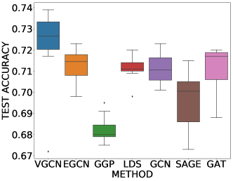
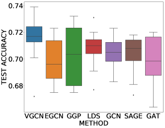
Figure 1: Test accuracy for the no-graph case on citeseer (left) and cora (right) across ten replications for our method (vgcn) and competing algorithms. The first three methods are Bayesian, while the others are not.

The benefits of our approach are less pronounced on cora as seen on the right of fig. 1, while we still see a marginal improvement over the other baselines. We attribute these differences between the datasets to the types of features used, bow vs tf-idf. Overall we can conclude that our method does manage to discover new graph parameterizations that improve performance even over methods that were specifically designed to do so, such as the lds algorithm of [17]. We also note that, as reported in [17], a dense gcn that does not use the graph (corresponding to a multi-layer Perceptron) achieves test accuracies of 58.4% and 59.1% on citeseer and cora respectively.

4.3 Results in the adversarial setting

We consider the robustness of vgcn and the baselines in the adversarial setting where the ground truth graph has been corrupted via the removal or addition of edges. Specifically, we consider the graph poisoning setting as outlined in [5] where the graph is poisoned before model training. We limit our study on general attacks where the attacker uses an unsupervised approach to perturb network structure and is not targeted to a classification task. In [5], it was shown that poisoning the network structure reduces performance on downstream tasks and transfers across to graph convolutional methods. These graph poisoning attacks are the easiest for an attacker to deploy in practice.

We applied graph poisoning on all 3 of our datasets removing 2,000, 1,000, and 500 edges (denoted using negative values in the figures) and also adding 500, 1000, 2,000, and 5,000 edges. We generated 10 attacked graphs for each of these settings. We note that removing 5,000 edges is not actually possible on citeseer hence we do not consider this setting. We show results for the extreme cases -2,000, 2,000, and 5,000 here and for all settings in the supplement.

Citation Networks: Figure 2 (left and middle) shows results for attacked graphs with node features, namely the two citation networks. We see that all methods perform well in the -2000 setting where the graphs are missing edges but all remaining edges are uncorrupted. The Bayesian methods vgcn and egcn have an advantage over the others on citeseer but the algorithms’ performance is more leveled up on cora. We note that performance for all methods degrades when false edges are added to the graphs. vgcn is the most robust especially in the extreme case of adding 5000 edges, effectively doubling the total number of edges in the graphs for both datasets. vgcn outperforms rgcn, which was specifically designed for these types of problems, especially in the cases of adding edges. Lastly, we note that variance for vgcn is lower across all graphs and datasets.

Featureless Graphs: Finally, we evaluate the performance of all methods on a graph without node features. Figure 2 (right) shows results for the polblogs network where node features are not available. All methods perform competitively across all attacked graph settings. Surprisingly, methods such as graphsage and graph attention network (gat) show superior performance for the -2000 setting but have very high variance at the 5000 regime. rgcn performs best when removing edges but does poorly when adding edges due to its heavy reliance on the similarity of node features.

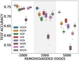
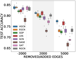
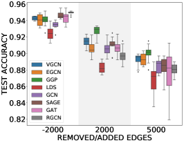
Figure 2: Test accuracy for the adversarial setting on attributed graphs citeseer (left) and cora (middle) and featureless graph polblogs (right) when removing (negative values) or adding (positive values) edges. Our method is denoted by vgcn.

While the Bayesian methods, vgcn, egcn, and ggp are the most robust on this dataset, lds is the worst performer across all graphs. One possible explanation for this is that the lack of node features negatively affects methods that optimize the graph structure as there may not be enough information in the training data and the graph structure alone to optimize the models with higher learning capacities, i.e., more parameters. Furthermore, we note that since the ground truth graph has approximately 16,000 edges, the 5000 fake edges are only an additional  30% as compared to nearly doubling of the number of edges for the citation networks. For higher levels of noise, Bayesian methods might demonstrate higher levels of robustness.

4.4 Performance on ground-truth graphs and qualitative analysis

Performance on ground-truth graphs.  Figure 3 shows the results for the ground-truth (unperturbed) graphs, where we see that vgcn can provide state-of-the-art performance, indicating that it can find better configurations even for those graphs that are believed to be most beneficial for the semi-supervised node classification task.

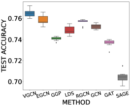
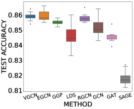
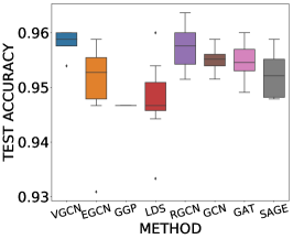
Figure 3: From left to right: Test accuracy for ground-truth graphs on citeseer, cora and polblogs across ten replications for our method (vgcn) and competing algorithms.

Limit posterior probabilities.  Here we analyze what our model has learned and how different the resulting posterior is with respect to the prior and its initialization during optimization. Interpreting Concrete distributions can be cumbersome so instead we use their zero-temperature property as presented in [35]. More specifically, in the zero-temperature limit, one can obtain the corresponding Bernoulli parameters of their discrete counterpart using $p(\text{lim}_{\tau\rightarrow 0}A_{ij}=1)={\lambda_{ij}}/{(\lambda_{ij}+1)}$. We refer to these probabilities as the limit posterior probabilities. Figure 4 (left) shows a histogram of these limit probabilities on a typical run of our model in the no-graph case for the citeseer dataset. As the majority of the links are close to zero, fig. 4 (left) only shows those probabilities that changed significantly with respect to the prior (defined as their absolute difference being greater than $0.02$). Hence, we see that in effect our algorithm manages to both decrease and increase these initial probabilities, providing evidence that it has the capacity to turn links on/off in the original graph. More precisely, the number of links with a significant change in their probabilities of being turned on was 3046. We believe this is indeed a significant amount, considering that the k-nearest neighbor graph had around 33,000 links and that the ‘true’ citeseer graph has around 4600 edges.

Learned graphs.  We illustrate the types of graphs learned by our approach by using an example from the adversarial setting experiment on citeseer when adding edges, where our approach significantly outperformed the competing baselines. Since showing the entire graph would be unintelligible, we enumerate communities (subgraphs that are internally densely connected) that contain a good balance of node labels. In particular, we use label propagation [58] to detect the largest communities and draw a graph for each. We show an example subgraph in fig. 4 (middle and right). On the middle we denote the edges from the original graph in solid lines and the added edges in dashed red lines. On the right is the corresponding complete graph with edge opacity proportional to their limit posterior probabilities. Generally speaking, the posterior probabilities of the original edges can be expected to remain largely the same or in some cases, either amplified or attenuated to improve downstream classification accuracy. More interestingly, we see that, with few exceptions (highlighted in red), the posterior probabilities of the added edges are attenuated. We show more example subgraphs in the supplement.

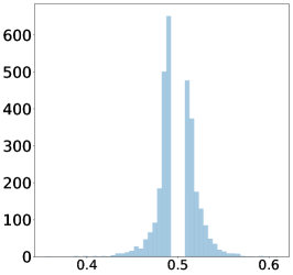
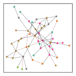
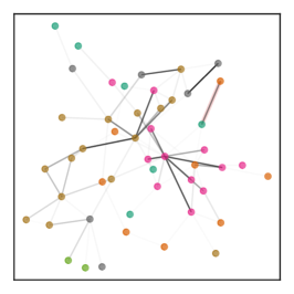
Figure 4: Left: Histogram of limit posterior probabilities of a link being turned on computed as the zero-temperature limit of the final variational posterior distributions over each adjacency entry (see text for details), using the citeseer dataset under the no-graph scenario. Middle: A community in the original graph from the adversarial citeseer experiment with node labels distinguished by colors and added edges denoted by red dashes. Right: Learned graph with edge opacity proportional to limit posterior probabilities. Added edges with probability greater than $\nicefrac{{1}}{{2}}$ are highlighted red.

5 Conclusion & discussion

We have presented variational graph convolutional networks (vgcns)for semi-supervised classification, a method that generalizes the capabilities of gcns by making them applicable in the absence of graph data and more robust to adversarial attacks. vgcn considers prior distributions over the graph along with a gcn likelihood in a joint probabilistic model and infers a graph posterior exploiting Concrete distributions. We have showcased the performance of our method on the above problems and using the ground-truth graphs. Our method can be extended beyond gcns to use other graph neural network architectures as long as the graph is represented by an adjacency matrix and that parameter estimation in the original method can be combined easily with variational inference.

Broader Impact

There exist numerous useful applications for graph-cnn s including e-commerce product recommendations [50], online social network recommendations [54], drug discovery [34, 41, 18], computational pharmacology [59], disease understanding [48], bioinformatics [16], finance [21], anti-money laundering [51], online hate speech classification [45], and understanding online fake news propagation [39].

Of the above applications, several can benefit from vgcn over existing graph-cnn s. Any application where there is incentive for bad actors to poison the data in order to (a) hide their activities, e.g., online hate speech, (b) control the activities of others, e.g., trick consumers into purchasing unreliable or expensive products, or (c) promote misinformation, e.g., fake news, stand to benefit from vgcn’s ability to deal with adversarial attacks.

Furthermore, vgcn is directly applicable to non-graph domains via the ad hoc construction of graphs hence the benefits of graph-cnn s can be brought into domains where data is not inherently graph-structured. As we have discussed earlier, such ad hoc graph creation results in noisy graphs requiring the use of principled structure modeling for training useful predictive models.

Just like any machine learning algorithm can be used for good it can also be used for harm. Graph-cnn s and our method vgcn are not immune to such misuse. For example, understanding how vgcn deals with adversarial attacks can be used by an adversarial agent to create more robust attacks and subvert attempts at detection. Currently, we have no solution for such a general problem but we understand that this needs to be addressed in future work.

Overall, we believe that our work is beneficial to society because of the many important applications that stand to benefit from vgcn’s ability to handle noise in the graph structure.

Appendix A Variational distributions

In this section we provide more details about the choices of variatiational distributions over the graph structure.

A.1 Variational distribution: free vs smooth parameterizations

Similarly to the prior definition, our approximate posterior is of the form

$$q_{{\boldsymbol{\mathbf{\phi}}}}({\boldsymbol{\mathbf{A}}})=\prod_{ij}q_{\boldsymbol{\mathbf{\phi}}}(A_{ij}),\text{ with }\quad q_{{\boldsymbol{\mathbf{\phi}}}}(A_{ij})=\mathrm{Bern}(A_{ij}\,|\,\rho_{ij}),\rho_{ij}>0,$$ (A.1)

where, henceforth, we use ${\boldsymbol{\mathbf{\phi}}}$ to denote all the parameters of the variational posterior. In the case where $\rho_{ij}$ are free parameters then ${\boldsymbol{\mathbf{\phi}}}=\{\rho_{ij}\}$. We refer to this approach as the free parameterization We have found experimentally that such a parameterization can make optimization of the elbo wrt ${\boldsymbol{\mathbf{\phi}}}$ extremely difficult. Thus, one is forced to either use alternative representations of the posterior, or continuous relaxations of the discrete prior and posterior distributions (see § A.2). Intuitively, conditional independence in the posterior is a strong assumption and small changes in $\rho_{ij}$ will compete with each other to explain the data. Consequently, any continuous optimization algorithm will find it very challenging to find a good direction in this non-smooth combinatorial space. Therefore, as an alternative, it is sensible to adopt a smooth parameterization:

$$\rho_{ij}=\sigma({\boldsymbol{\mathbf{z}}}_{i}^{T}\tilde{{\boldsymbol{\mathbf{z}}}}_{j}+b_{i}+b_{j}+s),{\boldsymbol{\mathbf{z}}}_{i},\tilde{{\boldsymbol{\mathbf{z}}}}_{j}\in\mathbb{R}^{d_{z}},\{b_{i},s\in\mathbb{R}\},$$ (A.2)

$i,j=1,\ldots,N$, where $\sigma(x)\equiv(1+\exp(-x))^{-1}$ is the logistic sigmoid function and $d_{z}\leq D$ is the dimensionality of the parameters ${\boldsymbol{\mathbf{z}}},\tilde{{\boldsymbol{\mathbf{z}}}}$. As we see, the same representation is shared across the columns and rows of ${\boldsymbol{\mathbf{A}}}$’s Bernoulli parameters, which addresses the combinatorial nature of the optimization landscape of the free parameterization. We note that this parameterization is referred to in the matrix-factorization and link-prediction literature as low-rank [37, 36] or dot-product [31]. In this case the variational parameters are ${\boldsymbol{\mathbf{\phi}}}=\{\{{\boldsymbol{\mathbf{z}}}_{i},\tilde{{\boldsymbol{\mathbf{z}}}}_{i},b_{i}\},s\}$.

A.2 Variational distribution: discrete vs relaxed

We have defined above a variational distribution which naturally models the discrete nature of the adjacency matrix ${\boldsymbol{\mathbf{A}}}$. Our goal is to estimate the parameters ${\boldsymbol{\mathbf{\phi}}}$ of the posterior $q_{{\boldsymbol{\mathbf{\phi}}}}({\boldsymbol{\mathbf{A}}})$ via maximization of the elbo. For this purpose we can use the so-called score function method [42], which provides an unbiased estimator of the gradient of an expectation of a function using mc samples. However, it is now widely accepted that, because of its generality, the score function estimator can suffer from high variance [43].

Therefore, as an alternative to the score function estimator, we can use the so-called re-parameterization trick [29, 44], which generally exhibits lower variance. Unfortunately, the re-parameterization trick is not applicable to discrete distributions so we need to resort to continuous relaxations. In this work we use Concrete distributions as proposed by Jang et al., [25], Maddison et al., [35]. In particular, we denote our binary Concrete posterior distribution with location parameters $\lambda_{ij}>0$ and temperature $\tau>0$ as $q_{{\boldsymbol{\mathbf{\phi}}}}(A_{ij})=\mathrm{BinConcrete}(A_{ij}\,|\,\lambda_{ij},\tau)$. Analogously, as discussed in Maddison et al., [35], in order to maintain a lower bound during variational inference we also relax our prior so that $p(A_{ij})=\mathrm{BinConcrete}(A_{ij}\,|\,\lambda^{o}_{ij},\tau_{o})$. In this case the variational parameters are the parameters of the Concrete distribution which can be, as in the discrete case, free parameters ${\boldsymbol{\mathbf{\phi}}}=\{\lambda_{ij}\}$ or have a smooth parameterization analogous to that in eq. A.2, i.e. $\lambda_{ij}=\exp({\boldsymbol{\mathbf{z}}}_{i}^{T}{\boldsymbol{\mathbf{z}}}_{j}+b_{i}+b_{j}+s)$ and, consequently, ${\boldsymbol{\mathbf{\phi}}}=\{\{{\boldsymbol{\mathbf{z}}}_{i},b_{i}\},s\}$.

Appendix B Binary discrete distributions

The kl divergence between two Bernoulli distributions $q(a\,|\,\rho)$ and $p(a\,|\,\rho^{o})$ can be computed as

$$\textsc{kl}\left[q(a\,|\,\rho)\;\|\;p(a\,|\,\rho^{o})\right]=\rho[\log\rho-\log\rho^{o}]+(1-\rho)[\log(1-\rho)-\log(1-\rho^{o})].$$ (B.1)

Appendix C Binary concrete distributions

In this section we give details of the re-parameterization used for the implementation of our algorithm when both the prior and the approximate posterior are relaxed via the binary Concrete distribution [35, 25].

C.1 Summary of Bernoulli relaxation transformations

$$A_{ij} \sim\mathrm{BinConcrete}(\lambda_{ij},\tau)\quad\Leftrightarrow\quad A_{ij}=\sigma(B_{ij}),\quad B_{ij}\sim\mathrm{Logistic}\left(\frac{\log\lambda_{ij}}{\tau},\frac{1}{\tau}\right);$$ (C.1)

$$B_{ij} \sim\mathrm{Logistic}\left(\frac{\log\lambda_{ij}}{\tau},\frac{1}{\tau}\right)\quad\Leftrightarrow\quad B_{ij}=\frac{\log\lambda_{ij}+L}{\tau},\quad L\sim\mathrm{Logistic}(0,1);$$ (C.2)

$$L \sim\mathrm{Logistic}(0,1)\quad\Leftrightarrow\quad L=\sigma^{-1}(U):=\log U-\log(1-U),\quad U\sim\mathrm{Uniform}(0,1).$$ (C.3)

In summary, we have

$$A_{ij}\sim\mathrm{BinConcrete}(\lambda_{ij},\tau)\quad\Leftrightarrow\quad A_{ij}=\sigma\left(\frac{\log\lambda_{ij}+\sigma^{-1}(U)}{\tau}\right)\quad U\sim\mathrm{Uniform}(0,1).$$ (C.4)

C.2 Re-parameterized elbo

With the results above, it is easy to see that we can write the elbo as:

$$\mathcal{L}_{\textsc{elbo}}({\boldsymbol{\mathbf{\phi}}}) =\mathbb{E}_{q_{{\boldsymbol{\mathbf{\phi}}},\tau}({\boldsymbol{\mathbf{A}}})}\left[\log p_{{\boldsymbol{\mathbf{\theta}}}}({\boldsymbol{\mathbf{Y}}}^{o}\,|\,{\boldsymbol{\mathbf{X}}},{\boldsymbol{\mathbf{A}}})-\log\frac{q_{{\boldsymbol{\mathbf{\phi}}},\tau}({\boldsymbol{\mathbf{A}}})}{p_{\tau_{o}}({\boldsymbol{\mathbf{A}}})}\right]$$ (C.5)

$$=\mathbb{E}_{g_{{\boldsymbol{\mathbf{\phi}}},\tau}({\boldsymbol{\mathbf{B}}})}\left[\log p_{{\boldsymbol{\mathbf{\theta}}}}({\boldsymbol{\mathbf{Y}}}^{o}\,|\,{\boldsymbol{\mathbf{X}}},\sigma({\boldsymbol{\mathbf{B}}}))-\log\frac{q_{{\boldsymbol{\mathbf{\phi}}},\tau}(\sigma({\boldsymbol{\mathbf{B}}}))}{p_{\tau_{o}}(\sigma({\boldsymbol{\mathbf{B}}}))}\right]$$ (C.6)

$$=\mathbb{E}_{g_{{\boldsymbol{\mathbf{\phi}}},\tau}({\boldsymbol{\mathbf{B}}})}\left[\log p_{{\boldsymbol{\mathbf{\theta}}}}({\boldsymbol{\mathbf{Y}}}^{o}\,|\,{\boldsymbol{\mathbf{X}}},\sigma({\boldsymbol{\mathbf{B}}}))-\log\frac{g_{{\boldsymbol{\mathbf{\phi}}},\tau}({\boldsymbol{\mathbf{B}}})}{f_{\tau_{o}}({\boldsymbol{\mathbf{B}}})}\right].$$ (C.7)

where

$$g_{{\boldsymbol{\mathbf{\phi}}},\tau}(B_{ij})=\mathrm{Logistic}\left(B_{ij}\,|\,\frac{\log\lambda_{ij}}{\tau},\frac{1}{\tau}\right),\quad f_{\tau_{o}}(B_{ij})=\mathrm{Logistic}\left(B_{ij}\,|\,\frac{\log\lambda^{o}_{ij}}{\tau_{o}},\frac{1}{\tau_{o}}\right).$$ (C.8)

C.3 Importance-weighted elbo

For the relaxed version of our algorithm (that uses binary Concrete distributions), in which we cannot compute the KL term in the elbo analytically, we use the importance-weighted elbo, which has been shown to perform better than the standard elbo, be a tighter bound of the marginal likelihood and related to variational inference in an augmented space [9, 15]:

$$\textsc{iw-elbo}=\sum_{{\boldsymbol{\mathbf{y}}}_{n}\in{\boldsymbol{\mathbf{Y}}}^{o}}\textsc{lme}_{{\boldsymbol{\mathbf{A}}}_{1:S}}\left[\log p({\boldsymbol{\mathbf{y}}}_{n}|{\boldsymbol{\mathbf{X}}},{\boldsymbol{\mathbf{A}}})-\frac{1}{|{\boldsymbol{\mathbf{Y}}}^{o}|}\log\frac{q_{{\boldsymbol{\mathbf{\phi}}},\tau}({\boldsymbol{\mathbf{A}}})}{p_{\tau_{o}}({\boldsymbol{\mathbf{A}}})}\right],$$ (C.9)

where $\textsc{lme}_{{\boldsymbol{\mathbf{A}}}_{1:S}}(h({\boldsymbol{\mathbf{A}}}))$ is the log-mean-exp operator of function $h({\boldsymbol{\mathbf{A}}})$ over samples of ${\boldsymbol{\mathbf{A}}}$, i.e. $\textsc{lme}_{{\boldsymbol{\mathbf{A}}}_{1:S}}=\log\frac{1}{S}\sum_{s=1}^{S}\exp(h({\boldsymbol{\mathbf{A}}}^{(s)}))$ with ${\boldsymbol{\mathbf{A}}}_{1:S}\equiv({\boldsymbol{\mathbf{A}}}^{(1)},\ldots,{\boldsymbol{\mathbf{A}}}^{(S)})$ and ${\boldsymbol{\mathbf{A}}}^{(s)}\sim q_{{\boldsymbol{\mathbf{\phi}}},\tau}({\boldsymbol{\mathbf{A}}})$.

Appendix D Implementation and computational complexity

We implement our approach using TensorFlow [1] for efficient GPU-based computation and also use some components of TensorFlow Probability [14]. The time complexity of our algorithm can be derived from considering the two main components of the elbo in eq. 5, namely the kl divergence term and the ell term. We focus here on one-hidden layer gcn (apart from the output layer) with dimensionality $Q\equiv Q^{(1)}$ along with a smooth (dot product) parameterization of the posterior. We recall that $N$ is the number of nodes, $D$ is the dimensionality of the input features ${\boldsymbol{\mathbf{X}}}$, $d_{z}$ is the dimensionality of posterior parameters ${\boldsymbol{\mathbf{Z}}}$, $C$ is the number of classes and $S$ is the number of samples from the variational posterior used to estimate the required expectations.

kl divergence term: We require to compute $\mathcal{O}(N^{2})$ individual kl divergences, which can be trivially parallelized. In the case of the smooth parameterization, for both the discrete and the relaxed cases, we need to compute the dot-product between the latent representations for each each $A_{ij}$ which is $\mathcal{O}(d_{z})$ and gradient information must be aggregated for each ${\boldsymbol{\mathbf{z}}}_{i},\tilde{{\boldsymbol{\mathbf{z}}}}_{i}$. While for a discrete posterior these individual kl terms can be computed exactly (as shown in appendix B), for the continuous relaxation we need to resort to mc estimation over $S$ samples. Aggregation over samples can also be parallelized straightforwardly.

ell term: Computing the ell using a 2-layer gcn as in eq. 1 requires $\mathcal{O}(NDQ+S(NQC+N^{2}Q+N^{2}C))$ for the continuous case. However, in the discrete case it only requires doing a forward pass over the standard gcn architecture $S$ times, hence being linear in the number of edges, i.e. $\mathcal{O}(S|\mathcal{E}|DQC)$, where $|\mathcal{E}|$ is the expected number of edges sampled from the posterior, assuming sparse-dense matrix multiplication is exploited.

Appendix E Datasets

Table 1 gives details of the datasets used in our experiments. Training/Valid/Test refer to the default training/validation/test set sizes. However, as mentioned in § 4, we adopt a similar approach to that of Franceschi et al., [17] where the training set is augmented with approximately 50% of the validation set.

Table 1: Datasets used in the experiments. Train/Valid/Test correspond the the training/validation/test set sizes. Label rate refers to the ratio of the training set size over the total number of nodes.

Dataset	Type	Nodes	Edges	Classes	Features	Train/Valid/Test	Label rate
cora	Citation network	2,708	5,278	7	1,433	140/500/1,000	0.052
citeseer	Citation network	3,327	4,676	6	3,703	120/500/1,000	0.036
polblogs	Blog network	1,222	16,717	2	N/A	122/275/825	0.10
pubmed	Citation network	19,717	44,338	3	500	60/500/1,000	0.003

Appendix F Full details of experimental set-up

Unless stated explicitly below, all the optimization-based methods were trained up to a maximum of 5,000 epochs using the Adam optimizer [28] with an initial learning rate of $0.001$. Hyper-parameter exploration was done via grid search and model selection carried out via cross-validation using the accuracy on the validation set. For standard gcn and our method we use a two-layer gcn as given in eq. 1 with a $16$-unit hidden layer. We train standard gcn as done by Kipf and Welling, [32] so as to minimize the cross-entropy loss, using dropout and L2 regularization, Glorot weight initialization [19] and row-normalization of input-feature vectors. As with our method, we set the dropout rate to $0.5$ and the regularization parameter in $\{5\times 10^{-3},5\times 10^{-4}\}$.

For our method, we carried posterior estimation over the adjacency matrix and MAP estimation of the gcn-likelihood parameters so as to maximize the elbo in eq. 5. Hyper-parameters for gcn-estimation were the same as above. To construct the prior over the adjacency matrix we followed the procedure explained in § 2.2 with $\bar{\rho}_{1}=\{0.25,0.5,0.75,0.99\}$, $\bar{\rho}_{0}=10^{-5}$, $\tau_{o}=\{0.1,0.5\}$, $\tau=\{0.1,0.5,0.66\}$ and $\beta=\{10^{-4},10^{-3},10^{-2},1\}$. We initialized the posterior to the same smoothed probabilities in the prior and used $S_{\text{train}}=3$ and $S_{\text{pred}}=16$ samples for estimating the required expectations for training and predictions, respectively. In the no-graph case all the methods explored k-nngs with $k=\{10,20\}$ and distance metrics $\{\text{cosine},\text{Minkowski}\}$.

For lds we used the code provided by the authors, which carries out bilevel optimization of the regularized cross-entropy loss and does model selection based on the validation accuracy using grid search across a range of parameters such as learning rates (for inner and outer objectives), number of neighbors and distance metrics. Similarly, for ggp and egcn we used the code provided by the authors.

For rgcn we used the code provided by the authors. For all experiments, we used the default parameters as described in [57]. Specifically, we used 2 hidden graph convolutional layers with $32$ units each and dropout 0.6. All models were trained for a maximum $200$ epochs with early stopping (20 epochs patience) using the Adam optimizer and an initial learning rate of $0.01$.

We used our own implementation of gat and graphsage. gat used an architecture identical to the one described in Veličković et al., [49]. The first layer consists of $K=8$ attention heads computing $F=8$ features, followed by an exponential linear unit (ELU) nonlinearity. The second layer is used for classification that computes $C$ features (where $C$ is the number of classes), followed by a softmax activation. $L2$ regularization with $\lambda=0.0005$ and $0.6$ dropout was used. The implementation of graphsage used mean aggregator functions and sampled the neighborhood at a depth of $K=2$ with neighborhood sample size of $S_{1}=25,S_{2}=10$ and batch size of $50$. The model was trained with 0.5 dropout and $L2$ regularization with $\lambda=0.0005$.

Appendix G Complete set of results for the adversarial setting

Here we include the complete set of experiments for the 7 attacked graphs removing 2000, 1000, and 500 edges as well as adding 500, 1000, 2000, and 5000 edges to the ground truth graphs. Figure 5 shows the results for all graphs.

On the citation networks, citeseer and cora, our proposed vgcn outperforms all other Bayesian and non-Bayesian methods, especially in the case of adding edges. On the polblogs network that is lacking node features, all methods perform similarly with ggp having a small edge in the cases of adding 2000 and 5000 edges. Our method, displays the lowest variance across all datasets.

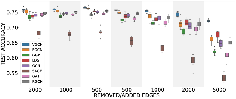
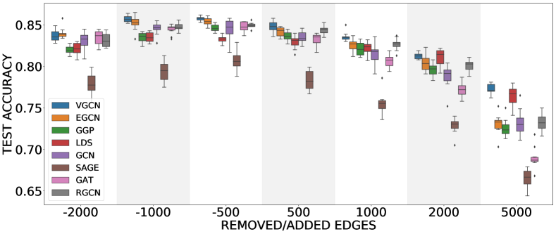
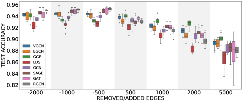
Figure 5: Results for the adversarial setting on attributed graphs citeseer (top), cora (middle), and (featureless graph) polblogs (bottom): Accuracy on the test set across ten attacked graphs at each attack setting such that negative values indicate removing edges and positive values adding edges. We compare our method (vgcn) with competing algorithms.

Appendix H Low-rank vs free parameterizations

Figure 6 compares the low-rank parameterization vs the free parameterization of our model, where we used a latent representation of dimensionality $d_{z}=100$. Our goal is to analyze whether a much more compact representation can yield similar results to those obtained by the free parameterization. For the citation networks used, the number of latent variables with the low-rank parameterization is $N\times 2\times d_{z}\approx 6\times 10^{5}$, whereas with the free parameterization we have $N\times(N-1)/2\approx 4.5\times 10^{6}$ latent variables. i.e. in this setting, the low-rank parameterization has an order of magnitude fewer latent variables. We see, in fig. 6, that although the low-rank parameterization can in some cases achieve a performance close to that of the free-parameterization, it also has a much higher variance and in most cases the resulting solution is considerably poorer. Nevertheless, we believe that factors such as initialization can improve the performance of the low-rank parameterization significantly and leave a much more thorough study of this for future work.

Appendix I Discrete vs relaxed

Besides the number of latent variables used to represent the posterior, we also want to investigate the effect of using the discrete Bernoulli distributions along with the score function estimators versus the relaxed binary Concrete distributions and the reparameterization trick. Figure 7 shows the performance of these two approaches on the citations networks under study and the no-graph case when using only $S=3$ posterior samples for prediction. We see that there is not much difference between the two approaches, although the relaxed version exhibits some outliers on citeseer (which is ameliorated when using $S=16$ samples) and the discrete version has slightly higher variance on cora. However, as we see in fig. 8, the relaxed version converges much faster than the discrete version, hence our selection of the former for our main results.

Figure 9 shows results of the discrete vs relaxed parameterization in the adversarial setting for the citeseer and cora datasets. Both models were trained for a maximum 5000 epochs with hyper-parameter optimization and model selection as described in appendix F. In the adversarial setting, there is an advantage to using the relaxed parameterization as it clearly outperforms the discrete one across all attack settings and both datasets. The difference in performance is more pronounced for citeseer. Lastly, the relaxed parameterization exhibits lower variance across all graphs.

Appendix J The Effect of the number of posterior samples on predictions

Figure 10 shows results for our model when using $S=3$ and $S=16$ samples from the posterior when making predictions. We observe that, as expected, using more posterior samples does improve performance and that the additional gains of using more samples are worthwhile if the computational constrains can be satisfied.

Appendix K The influence of the KL term during training

As mentioned in the main paper, we scaled the kl term by a dampening factor $\beta<1$ so that it does not dominate the likelihood term in the elbo. We have analyzed this KL-dampening factor on the adversarial experiments across all datasets. Figure 11 shows how frequently each factor was selected through cross-validation with $\beta=\{1,10^{-2},10^{-3},10^{-4}\}$ being selected $\{32\%,35\%,21\%,12\%\}$ of the time, respectively. Along with the performance benefits shown in the main paper, this confirms that KL regularization resulting from variational inference does have an effect. Lastly, we have found that even when $\beta$ is very small, the kl term still has an effect as it can be several orders of magnitude larger than the ell.

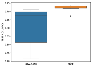
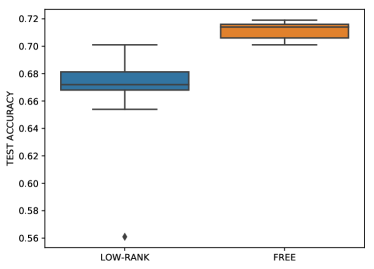
Figure 6: Results in the no-graph case for citeseer (left) and cora (right)—low-rank vs free parameterization: The test accuracy of our method (vgcn) using a low-rank parameterization and a free parameterization, with the latent dimensionality of the low-rank parameterization $d_{z}=100$. As with the results in the main paper, In both cases we used $S_{\text{pred}}=16$ posterior samples for predictions.

Figure 7: Results in the no-graph case for citeseer (left) and cora (right)—discrete vs relaxed: The test accuracy of our method (vgcn) using a free parameterization with discrete Bernoulli distributions and relaxed binary Concrete distributions. Unlike the results in the main paper, in both cases we used $S_{\text{pred}}=3$ posterior samples for predictions.

Figure 8: Results in the no-graph case—convergence of discrete vs relaxed approaches on citeseer: Convergence of the free parameterization with the discrete and the relaxed version using $S_{\text{pred}}=3$ posterior samples for predictions.

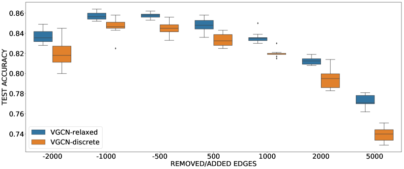
Figure 9: Results in the adversarial setting for citeseer (top) and cora (bottom) —discrete vs relaxed: The test accuracy of our method (vgcn) using a free parameterization with discrete Bernoulli distributions (vgcn-discrete) and relaxed binary Concrete distributions (vgcn-relaxed). In both cases we used $S_{\text{pred}}=3$ posterior samples for predictions.

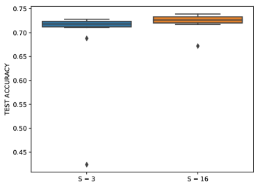
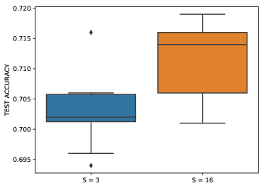
Figure 10: Results in the no-graph case for citeseer (left) and cora (right)—effect of the number of samples: The test accuracy of our method (vgcn) (with freely parameterized relaxed binary Concrete distributions) using $S\equiv S_{\text{pred}}=3$ and $S\equiv S_{\text{pred}}=16$ posterior samples for predictions.

Appendix L Posterior analysis in the adversarial setting

Similar to the analysis in fig. 3 of the main paper for the no-graph case, here we look at the posterior changes for a representative experiment in the adversarial setting. Figure 12 shows the difference between the final posterior probabilities obtained by our algorithm and the prior probabilities, which were also used to initialize the posterior. We see that our model manages to effectively turn off/turn on a significant number of links.

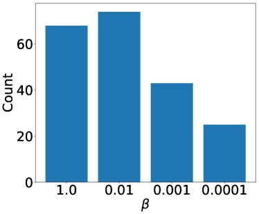
Figure 11: Histogram of kl-dampening factor $\beta$ selected using cross-validation for experiments using the citeseer, cora, and polblogs datasets, where $\beta=1$ accounts for no dampening of the kl term in the elbo.

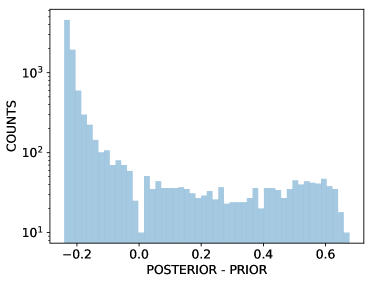
Figure 12: Posterior changes in the adversarial setting on citeseer. The difference in the limit probabilities computed as the zero-temperature limit of the final variational posterior distributions over each adjacency entry. Only showing those probabilities that changed significantly from the prior, which had a maximum value of $0.25$ and a minimum value of $10^{-5}$. The total number of changed probabilities was $9,504$.

Appendix M Additional examples of learned graphs

Following on from § 4.4 of the main paper, we visualize additional communities of the citeseer citation network with added edges and the corresponding latent graph inferred using our approach. We show four communities in fig. 13. As before, on the left we denote the edges from the original graph in solid lines and the added edges in dashed red lines; on the right is the corresponding complete graph with edge opacity drawn proportionally to the limit posterior probabilities.

Furthermore, let $E^{\prime}$ denote the set of added edges. If we have inferred a posterior that suppresses the negative influence of these added edges, we would expect that $\{i,j\}\in E^{\prime}$ implies $p(A_{ij})<\nicefrac{{1}}{{2}}$. On the right, we highlight in red every edge $\{i,j\}\in E^{\prime}$ where $p(A_{ij})\geq\nicefrac{{1}}{{2}}$. We can see that such cases are few and far between, even in communities predominantly consisting of added edges (e.g. row 3).

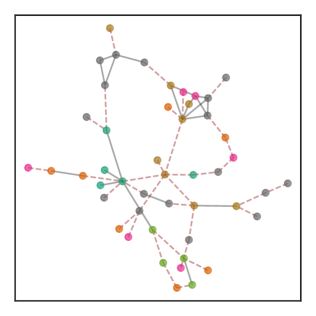
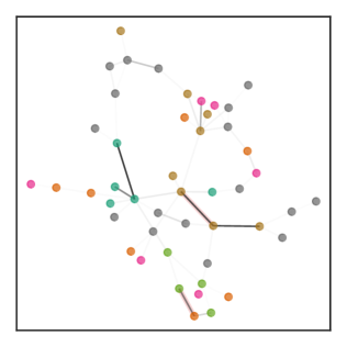
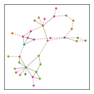
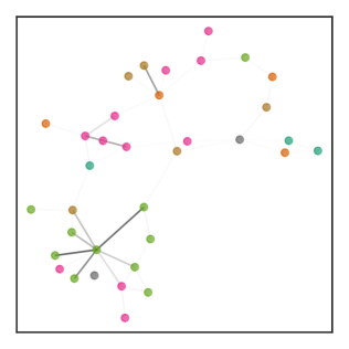
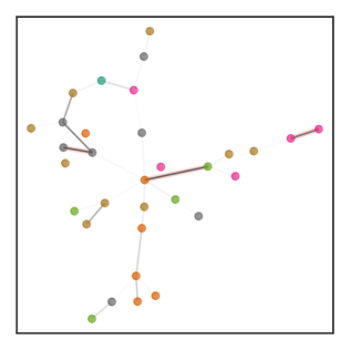
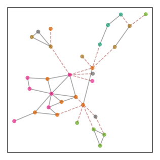
Figure 13: Left: Communities in the original graph from the adversarial citeseer experiment with node labels distinguished by colors and added edges denoted by red dashes. Right: Learned graph with edge opacity proportional to limit posterior probabilities. Added edges with probability greater than $\nicefrac{{1}}{{2}}$ are highlighted red.

Appendix N Results using random data splits

It was argued in [47] that model evaluation using pre-existing data train/validation/test splits produces overconfident estimates of a GNN model’s performance. It is thus suggested that random splits of the data should be instead used. Here we have repeated the experiments outlined in section  G using random splits and show the results in fig. 14. We have used the same random splits to evaluate all competing methods.

Comparing the results shown in fig. 5 and fig. 14, we notice that there is a small drop in performance for all methods and across all attack settings. However, overall our vgcn method continues to outperform the others especially in the setting of adding a large number of false edges. The egcn method has a small advantage over vgcn when removing $2000$ and $1000$ edges on both datasets; however, we note that the variance of egcn has also increased considerably when compared to the results using the fixed splits as shown in fig. 5. Overall, our original conclusions about the benefits of vgcn in the case of attacked graphs remain true regardless of how the given data is split for training and validation.

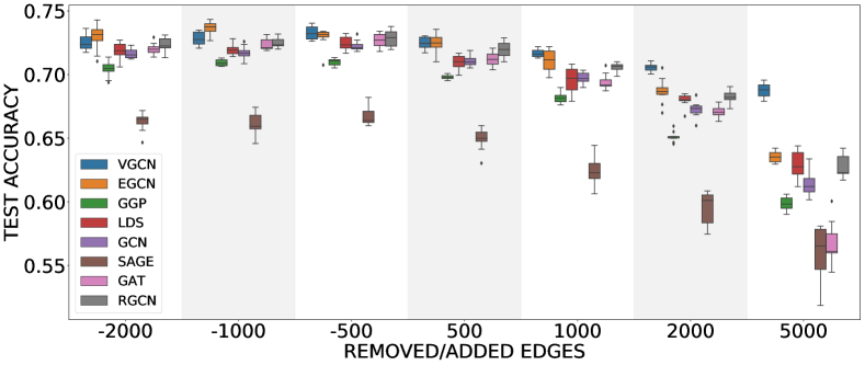
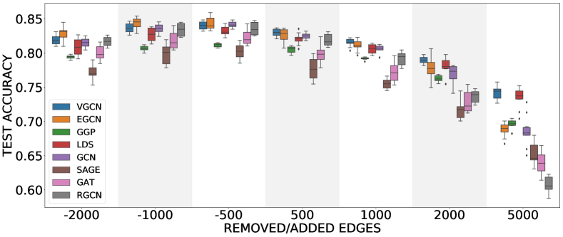
Figure 14: Results for the adversarial setting on attributed graphs citeseer (top), cora (bottom) using random splits of the data into train/validation/test sets: Accuracy on the test set across ten attacked graphs at each attack setting such that negative values indicate removing edges and positive values adding edges. We compare our method (vgcn) with competing algorithms.

Appendix O Mini-batch training

We explored mini-batch training employing the approach of [10]. Mini-batch training permits applying our method to larger datasets where the full-batch method would result in out-of-memory errors. An additional benefit is also an order reduction in the number of model parameters through a block-diagonal approximation of the given graph; this approach is referred to as vanilla cluster-gcn in [10]. We decompose the auxiliary graph into $m$ non-overlapping subgraphs using the METIS [27] algorithm. Then, we optimise the vgcn parameters using mini-batch SGD considering each subgraph as a mini-batch.

Figure 15 shows the performance of our method using mini-batch training with a block-diagonal approximation on the pubmed dataset in the adversarial setting. The statistics for the pubmed dataset are shown in Table 1. We can see that this is a much larger dataset than cora and citeseer. In the adversarial setting, we consider attacks that add or remove edges proportionally to the total number of edges in the ground truth graph such that we remove approximately 50% of the edges or add 50% or 100% of edges. For these experiments we limited the search space for the hyper-parameters to the following: gcn regularisation in $\{5\times 10^{-3},5\times 10^{-4}\}$, $\bar{\rho}_{1}=\{0.25,0.5,0.75\}$, $\beta=\{10^{-2},10^{-3}\}$, $\tau_{o}=\{0.5\}$, and $\tau=\{0.5,0.66\}$. Finally, we reduced the given graph to $20$ non-overlapping graphs.

In fig. 15 we compare vgcn with gcn, gat, and rgcn. We see that in the case of attacks that add edges to the graph, our vgcn method outperforms all others. In the case of attacks that remove edges, all methods have similar performance although vgcn displays a small performance drop and higher variance. This can easily be explained as an artifact of the block-diagonal approximation that forces vgcn to consider a much smaller set of edges than the other methods. That is, the number of edges removed are both the attacked ones as well as the between-subgraph edges.

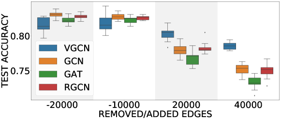
Figure 15: Results using mini-batch training with a block-diagonal approximation of the auxiliary graph on the Pubmed dataset in the adversarial setting.

References

- Abadi et al., [2015] Abadi, M., Agarwal, A., Barham, P., et al. (2015). TensorFlow: Large-scale machine learning on heterogeneous systems.
- Adamic and Glance, [2005] Adamic, L. A. and Glance, N. (2005). The political blogosphere and the 2004 us election: divided they blog. In Proceedings of the 3rd international workshop on Link discovery, pages 36–43.
- Airoldi et al., [2008] Airoldi, E. M., Blei, D. M., Fienberg, S. E., and Xing, E. P. (2008). Mixed membership stochastic blockmodels. Journal of Machine Learning Research, 9(Sep):1981–2014.
- Alemi et al., [2018] Alemi, A., Poole, B., Fischer, I., Dillon, J., Saurous, R. A., and Murphy, K. (2018). Fixing a broken ELBO. In International Conference on Machine Learning, pages 159–168.
- Bojchevski and Günnemann, [2019] Bojchevski, A. and Günnemann, S. (2019). Adversarial attacks on node embeddings via graph poisoning. In International Conference on Machine Learning.
- Boldi et al., [2012] Boldi, P., Bonchi, F., Gionis, A., and Tassa, T. (2012). Injecting uncertainty in graphs for identity obfuscation. Proceedings of the VLDB Endowment, 5(11):1376–1387.
- Bowman et al., [2016] Bowman, S., Vilnis, L., Vinyals, O., Dai, A., Jozefowicz, R., and Bengio, S. (2016). Generating sentences from a continuous space. In Proceedings of The 20th SIGNLL Conference on Computational Natural Language Learning, pages 10–21.
- Bruna et al., [2014] Bruna, J., Zaremba, W., Szlam, A., and Lecun, Y. (2014). Spectral networks and locally connected networks on graphs. In International Conference on Learning Representations.
- Burda et al., [2015] Burda, Y., Grosse, R., and Salakhutdinov, R. (2015). Importance weighted autoencoders. arXiv preprint arXiv:1509.00519.
- Chiang et al., [2019] Chiang, W.-L., Liu, X., Si, S., Li, Y., Bengio, S., and Hsieh, C.-J. (2019). Cluster-GCN: An efficient algorithm for training deep and large graph convolutional networks. In Proceedings of the 25th ACM SIGKDD International Conference on Knowledge Discovery & Data Mining, KDD ’19, page 257–266, New York, NY, USA. Association for Computing Machinery.
- Dallachiesa et al., [2014] Dallachiesa, M., Aggarwal, C., and Palpanas, T. (2014). Node classification in uncertain graphs. In International Conference on Scientific and Statistical Database Management. ACM.
- Defferrard et al., [2016] Defferrard, M., Bresson, X., and Vandergheynst, P. (2016). Convolutional Neural Networks on Graphs with Fast Localized Spectral Filtering. In Advances in Neural Information Processing Systems, pages 3844–3852.
- Dieng et al., [2019] Dieng, A. B., Kim, Y., Rush, A. M., and Blei, D. M. (2019). Avoiding latent variable collapse with generative skip models. In International Conference on Artificial Intelligence and Statistics, pages 2397–2405.
- Dillon et al., [2017] Dillon, J. V., Langmore, I., Tran, D., Brevdo, E., Vasudevan, S., Moore, D., Patton, B., Alemi, A., Hoffman, M., and Saurous, R. A. (2017). TensorFlow Distributions. arXiv preprint arXiv:1711.10604.
- Domke and Sheldon, [2018] Domke, J. and Sheldon, D. R. (2018). Importance weighting and variational inference. In Bengio, S., Wallach, H., Larochelle, H., Grauman, K., Cesa-Bianchi, N., and Garnett, R., editors, Advances in Neural Information Processing Systems 31, pages 4470–4479. Curran Associates, Inc.
- Fout et al., [2017] Fout, A., Byrd, J., Shariat, B., and Ben-Hur, A. (2017). Protein interface prediction using graph convolutional networks. In Advances in Neural Information Processing Systems, pages 6530–6539.
- Franceschi et al., [2019] Franceschi, L., Niepert, M., Pontil, M., and He, X. (2019). Learning discrete structures for graph neural networks. In International Conference on Machine Learning.
- Gilmer et al., [2017] Gilmer, J., Schoenholz, S. S., Riley, P. F., Vinyals, O., and Dahl, G. E. (2017). Neural message passing for quantum chemistry. In International Conference on Machine Learning, pages 1263–1272. JMLR.org.
- Glorot and Bengio, [2010] Glorot, X. and Bengio, Y. (2010). Understanding the difficulty of training deep feedforward neural networks. In Artificial Intelligence and Statistics, pages 249–256.
- Hamilton et al., [2017] Hamilton, W., Ying, Z., and Leskovec, J. (2017). Inductive representation learning on large graphs. In Advances in Neural Information Processing Systems, pages 1024–1034.
- Han et al., [2019] Han, X., Ding, R., Wang, L., and Huang, H. (2019). Creditprint: Credit investigation via geographic footprints by deep learning. arXiv preprint arXiv:1910.08734v1.
- Henaff et al., [2015] Henaff, M., Bruna, J., and LeCun, Y. (2015). Deep convolutional networks on graph-structured data. arXiv preprint arXiv:1506.05163.
- Higgins et al., [2017] Higgins, I., Matthey, L., Pal, A., Burgess, C., Glorot, X., Botvinick, M., Mohamed, S., and Lerchner, A. (2017). beta-VAE: Learning basic visual concepts with a constrained variational framework. In International Conference on Learning Representations.
- Hu et al., [2017] Hu, J., Cheng, R., Huang, Z., Fang, Y., and Luo, S. (2017). On embedding uncertain graphs. In Proceedings of the 2017 ACM on Conference on Information and Knowledge Management, pages 157–166. ACM.
- Jang et al., [2016] Jang, E., Gu, S., and Poole, B. (2016). Categorical Reparameterization with Gumbel-Softmax. arXiv preprint arXiv:1611.01144.
- Jordan et al., [1999] Jordan, M. I., Ghahramani, Z., Jaakkola, T. S., and Saul, L. K. (1999). An introduction to variational methods for graphical models. Machine learning, 37(2):183–233.
- Karypis and Kumar, [1998] Karypis, G. and Kumar, V. (1998). A fast and high quality multilevel scheme for partitioning irregular graphs. SIAM J. Sci. Comput., 20(1):359–392.
- Kingma and Ba, [2014] Kingma, D. P. and Ba, J. (2014). Adam: A method for stochastic optimization. arXiv preprint arXiv:1412.6980.
- Kingma and Welling, [2014] Kingma, D. P. and Welling, M. (2014). Auto-encoding variational Bayes. In International Conference on Learning Representations.
- Kipf et al., [2018] Kipf, T., Fetaya, E., Wang, K.-C., Welling, M., and Zemel, R. (2018). Neural relational inference for interacting systems. In International Conference on Machine Learning.
- Kipf and Welling, [2016] Kipf, T. N. and Welling, M. (2016). Variational graph auto-encoders. arXiv preprint arXiv:1611.07308.
- Kipf and Welling, [2017] Kipf, T. N. and Welling, M. (2017). Semi-Supervised Classification with Graph Convolutional Networks. In International Conference on Learning Representations.
- LeCun et al., [1998] LeCun, Y., Bottou, L., Bengio, Y., Haffner, P., et al. (1998). Gradient-based learning applied to document recognition. Proceedings of the IEEE, 86(11):2278–2324.
- Li et al., [2017] Li, J., Cai, D., and He, X. (2017). Learning graph-level representation for drug discovery. arXiv preprint arXiv:1709.03741v2.
- Maddison et al., [2017] Maddison, C. J., Mnih, A., and Teh, Y. W. (2017). The Concrete Distribution: A Continuous Relaxation of Discrete Random Variables. In International Conference on Learning Representations.
- Menon and Elkan, [2011] Menon, A. K. and Elkan, C. (2011). Link prediction via matrix factorization. In Joint European conference on machine learning and knowledge discovery in databases, pages 437–452. Springer.
- Mnih and Salakhutdinov, [2008] Mnih, A. and Salakhutdinov, R. R. (2008). Probabilistic matrix factorization. In Advances in Neural Information Processing Systems, pages 1257–1264.
- Monti et al., [2017] Monti, F., Boscaini, D., Masci, J., Rodola, E., Svoboda, J., and Bronstein, M. M. (2017). Geometric deep learning on graphs and manifolds using mixture model CNNs. In IEEE Conference on Computer Vision and Pattern Recognition, pages 5115–5124.
- Monti et al., [2019] Monti, F., Frasca, F., Eynard, D., Mannion, D., and Bronstein, M. M. (2019). Fake news detection on social media using geometric deep learning. ArXiv, abs/1902.06673.
- Ng et al., [2018] Ng, Y. C., Colombo, N., and Silva, R. (2018). Bayesian semi-supervised learning with graph Gaussian processes. In Advances in Neural Information Processing Systems, pages 1683–1694.
- Nguyen et al., [2020] Nguyen, T., Le, H., Quinn, T. P., Le, T., and Venkatesh, S. (2020). Predicting drug–target binding affinity with graph neural networks. bioRxiv.
- Ranganath et al., [2014] Ranganath, R., Gerrish, S., and Blei, D. M. (2014). Black box variational inference. In Artificial Intelligence and Statistics.
- Ranganath et al., [2016] Ranganath, R., Tran, D., and Blei, D. (2016). Hierarchical variational models. In International Conference on Machine Learning, pages 324–333.
- Rezende et al., [2014] Rezende, D. J., Mohamed, S., and Wierstra, D. (2014). Stochastic backpropagation and approximate inference in deep generative models. In International Conference on Machine Learning.
- Ribeiro et al., [2018] Ribeiro, M. H., Calais, P. H., Santos, Y. A., Almeida, V. A. F., and Meira, W. (2018). Characterizing and detecting hateful users on twitter. In ICWSM.
- Seshadhri et al., [2020] Seshadhri, C., Sharma, A., Stolman, A., and Goel, A. (2020). The impossibility of low-rank representations for triangle-rich complex networks. Proceedings of the National Academy of Sciences, 117(11):5631–5637.
- Shchur et al., [2018] Shchur, O., Mumme, M., Bojchevski, A., and Günnemann, S. (2018). Pitfalls of graph neural network evaluation. arXiv preprint arXiv:1811.05868.
- Sügis et al., [2019] Sügis, E., Dauvillier, J., Leontjeva, A., Adler, P., Hindie, V., Moncion, T., Collura, V., Daudin, R., Loe-Mie, Y., Herault, Y., Lambert, J.-C., Hermjakob, H., Pupko, T., Rain, J.-C., Xenarios, I., Vilo, J., Simonneau, M., and Peterson, H. (2019). Hena, heterogeneous network-based data set for alzheimer’s disease. Scientific Data, 6(1):151.
- Veličković et al., [2018] Veličković, P., Cucurull, G., Casanova, A., Romero, A., Liò, P., and Bengio, Y. (2018). Graph Attention Networks. In International Conference on Learning Representations.
- Wang et al., [2020] Wang, X., Salim, F. D., Ren, Y., and Koniusz, P. (2020). Relation embedding for personalised translation-based poi recommendation. In Lauw, H. W., Wong, R. C.-W., Ntoulas, A., Lim, E.-P., Ng, S.-K., and Pan, S. J., editors, Advances in Knowledge Discovery and Data Mining, pages 53–64, Cham. Springer International Publishing.
- Weber et al., [2018] Weber, M., Chen, J., Suzumura, T., Pareja, A., Ma, T., Kanezashi, H., Kaler, T., Leiserson, C. E., and Schardl, T. B. (2018). Scalable graph learning for anti-money laundering: A first look. CoRR, abs/1812.00076.
- Wu et al., [2019] Wu, Z., Pan, S., Chen, F., Long, G., Zhang, C., and Yu, P. S. (2019). A comprehensive survey on graph neural networks. arXiv preprint arXiv:1901.00596.
- Yang et al., [2016] Yang, Z., Cohen, W. W., and Salakhutdinov, R. (2016). Revisiting semi-supervised learning with graph embeddings. In International Conference on Machine Learning.
- Ying et al., [2018] Ying, R., He, R., Chen, K., Eksombatchai, P., Hamilton, W. L., and Leskovec, J. (2018). Graph convolutional neural networks for web-scale recommender systems. In Proceedings of the 24th ACM SIGKDD International Conference on Knowledge Discovery & Data Mining, KDD ’18, page 974–983, New York, NY, USA. Association for Computing Machinery.
- Zhang et al., [2019] Zhang, Y., Pal, S., Coates, M., and Üstebay, D. (2019). Bayesian graph convolutional neural networks for semi-supervised classification. In AAAI Conference on Artificial Intelligence.
- Zhou et al., [2018] Zhou, J., Cui, G., Zhang, Z., Yang, C., Liu, Z., and Sun, M. (2018). Graph neural networks: A review of methods and applications. arXiv preprint arXiv:1812.08434.
- Zhu et al., [2019] Zhu, D., Zhang, Z., Cui, P., and Zhu, W. (2019). Robust graph convolutional networks against adversarial attacks. In Proceedings of the 25th ACM SIGKDD International Conference on Knowledge Discovery & Data Mining, KDD ’19, page 1399–1407, New York, NY, USA. Association for Computing Machinery.
- Zhu and Ghahramani, [2003] Zhu, X. and Ghahramani, Z. (2003). Learning from labeled and unlabeled data with label propagation. Technical Report CMU-CALD-02-106, Carnegie Mellon University.
- Zitnik et al., [2018] Zitnik, M., Agrawal, M., and Leskovec, J. (2018). Modeling polypharmacy side effects with graph convolutional networks. Bioinformatics, 34(13):457–466.