Travelling Waves
for Reaction-Diffusion Equations
Forced by Translation Invariant Noise

Abstract

Inspired by applications, we consider reaction-diffusion equations on $\mathbb{R}$ that are stochastically forced by a small multiplicative noise term that is white in time, coloured in space and invariant under translations. We show how these equations can be understood as a stochastic partial differential equation (SPDE) forced by a cylindrical Q-Wiener process and subsequently explain how to study stochastic travelling waves in this setting. In particular, we generalize the phase tracking framework that was developed in [20, 19] for noise processes driven by a single Brownian motion. The main focus lies on explaining how this framework naturally leads to long term approximations for the stochastic wave profile and speed. We illustrate our approach by two fully worked-out examples, which highlight the predictive power of our expansions.

Physica D

, [coraut]Corresponding author. , [LD1] Mathematisch Instituut - Universiteit Leiden
P.O. Box 9512; 2300 RA Leiden; The Netherlands
Email: c.h.s.hamster@math.leidenuniv.nl [LD2] Mathematisch Instituut - Universiteit Leiden
P.O. Box 9512; 2300 RA Leiden; The Netherlands
Email: hhupkes@math.leidenuniv.nl

35K57 35R60 .

travelling waves, stochastic forcing, nonlinear stability, stochastic phase shift.

1 Introduction

In this paper we set out to study the propagation of wave solutions to stochastic equations of the form

$$\begin{split}u_{t}&=\rho\partial_{xx}u+f(u)+\sigma g(u)\xi(x,t),\\ \end{split}$$ (1.1)

in which $\xi$ is a Gaussian process that is white in time and coloured in space. In particular, we assume formally that

$$\begin{split}E[\xi(x,t)]&=0,\\ E[\xi(x,t)\xi(x^{\prime},t^{\prime})]&=\delta(t-t^{\prime})q(x-x^{\prime}),\end{split}$$ (1.2)

for some smooth covariance function $q$ that describes the correlation in space. Such equations have been used in a wide range of applications, for example to model the appearance of travelling waves in light-sensitive Belousov-Zhabotinsky chemical reactions [26] or to study the excitability of activator-inhibitor systems such as nerve fibres [15]. We refer to [16, §6.1] for an extended list of examples.

We will assume here that (1.1) with $\sigma=0$ admits a spectrally stable deterministic travelling front or pulse and examine the impact of the multiplicative noise term for small $\sigma$. The nonlinearity $g$ will be chosen to vanish at the endpoints of the deterministic wave. In particular, the full stochastic system is at rest whenever the deterministic portion is at rest. Such an assumption is typically used to examine the distortions on a system caused by external random effects, such as fluctuations in the intensity of the light driving a Belousov-Zhabotinsky reaction. In a controlled setting these effects can often be minimized or switched off completely, leading to the notion of the deterministic limit.

On the other hand, internal fluctuations arise from the microscopic properties of the system itself and cannot be readily eliminated. For example, the vibrations of the individual atoms are essential ingredients in the derivation of the ideal gas equations. It is more natural to use an additive noise term to model effects of this type, but we do not focus on this case here.

The main goal of this paper is to uncover the corrections to the deterministic wave that are caused by the (small) multiplicative noise term. In particular, we develop a framework that allows the corrections to the speed and shape of the wave to be computed to any desired order in $\sigma$. We explicitly compute the second and third order correction terms and show numerically that these expansions are valid for long time scales. We also outline in which sense these predictions can be made rigorous, which involves casting the translationally invariant Stochastic Partial Differential Equation (SPDE) (1.1) into a mathematically precise form.

Example I: The Nagumo equation

In order to set the stage, let us consider the stochastic Nagumo equation

$$\begin{split}u_{t}&=\rho\partial_{xx}u+f_{\mathrm{cub}}(u;\alpha)+\sigma u(1-u)\xi(x,t),\\ \end{split}$$ (1.3)

with the bistable cubic nonlinearity

$$f_{\mathrm{cub}}(u;\alpha)=u(1-u)(u-\alpha),\qquad\qquad 0<\alpha<1$$ (1.4)

and the Gaussian covariance kernel

$$q(x)=\frac{1}{2}e^{\frac{-\pi x^{2}}{4}}.$$ (1.5)

For $0<a<1$, the deterministic system is known to have a spectrally stable wave solution $u(x,t)=\Phi_{0}(x-c_{0}t)$ that connects the stable rest states zero and one [27]. In fact, the travelling wave ODE

$$\rho\Phi_{0}^{\prime\prime}+c_{0}\Phi_{0}^{\prime}+f_{\mathrm{cub}}(\Phi_{0};\alpha)=0$$ (1.6)

can be solved by using the explicit expressions

$$c_{0}=\sqrt{2\rho_{0}}\left(\frac{1}{2}-\alpha_{0}\right),\qquad\Phi_{0}(x)=\frac{1}{2}\left[1-\tanh\left(\frac{1}{2\sqrt{2\rho_{0}}}x\right)\right]$$ (1.7)

with $(\rho_{0},\alpha_{0})=(\rho,\alpha)$.

Note that the form of the nonlinear terms in (1.3) allows us to recast the system as

$$\begin{split}u_{t}&=\rho_{0}\partial_{xx}u+f_{\mathrm{cub}}\big{(}u;\alpha_{0}-\sigma\xi(x,t)\big{)},\\ \end{split}$$ (1.8)

showing that we are stochastically forcing the (external) parameter $\alpha$. As a consequence, it is natural to ask whether effective $\sigma$-dependent parameters $(\rho_{\sigma},\alpha_{\sigma})$ can be derived that are able to capture the stochastic effects on the waves by replacing (1.7) with

$$c_{\sigma}=\sqrt{2\rho_{\sigma}}\left(\frac{1}{2}-\alpha_{\sigma}\right),\qquad\Phi_{\sigma}(x)=\frac{1}{2}\left[1-\tanh\left(\frac{1}{2\sqrt{2\rho_{\sigma}}}x\right)\right].$$ (1.9)

In the case where $\xi(x,t)$ is replaced by the derivative of a single $x$-independent Brownian motion in time, this point of view can be made fully explicit and precise. Indeed, in this case the wave (1.9) with

$$(\rho_{\sigma},\alpha_{\sigma})=(\frac{\rho_{0}}{1+\sigma^{2}\rho_{0}},\alpha_{0})$$ (1.10)

is an exact solution to the underlying SPDE [20, 7], with a phase that follows a scaled Brownian motion.

The early results in [16] for general $\xi$ can also be seen in this light. Indeed, the authors use a formal (partial) expansion to suggest the choices

$$\rho_{\sigma}=\frac{1}{1-\sigma^{2}q(0)},\qquad\alpha_{\sigma}=\frac{2\alpha_{0}-\sigma^{2}q(0)}{2-2\sigma^{2}q(0)}$$ (1.11)

where $\rho_{0}=1$. However, the waves found in this way are only approximate solutions to (1.3). We show in §3 how our techniques can be used to significantly improve the quality of this approximation.

In order to discuss the stability of these waves, we introduce the linearised operator

$$\mathcal{L}_{\mathrm{tw}}v=\rho v^{\prime\prime}+c_{0}v^{\prime}+f_{\mathrm{cub}}^{\prime}(\Phi_{0};\alpha)v,$$ (1.12)

together with its formal adjoint

$$\mathcal{L}^{*}_{\mathrm{tw}}w=\rho w^{\prime\prime}-c_{0}w^{\prime}+f_{\mathrm{cub}}^{\prime}(\Phi_{0},\alpha)w.$$ (1.13)

By direct substitution, it can be verified that $\psi_{\mathrm{tw}}(\xi)=\kappa e^{c_{0}\xi/\rho}\Phi_{0}^{\prime}(\xi)$ is an element of the kernel of $\mathcal{L}^{*}_{\mathrm{tw}}$; see also [27, ex. 2.3.1 and 4.1.4] for more intuition. The constant $\kappa$ can be chosen in such a way that

$$\mathcal{L}_{\mathrm{tw}}\Phi_{0}^{\prime}=\mathcal{L}^{*}_{\mathrm{tw}}\psi_{\mathrm{tw}}=0,\qquad\langle\psi_{\mathrm{tw}},\Phi_{0}^{\prime}\rangle=1,$$ (1.14)

which allows us to write

$$Pv=\langle\psi_{\mathrm{tw}},v\rangle_{L^{2}}\Phi_{0}^{\prime}$$ (1.15)

for the spectral projection onto the simple zero eigenspace of $\mathcal{L}_{\mathrm{tw}}$.

Since the remainder of the spectrum of $\mathcal{L}_{\mathrm{tw}}$ lies strictly to the left of the imaginary axis, general considerations [36] can be used to show that the associated semigroup satisfies the bound

$$\left\|e^{\mathcal{L}_{\mathrm{tw}}t}(I-P)v\right\|_{L^{2}(\mathbb{R})}\leq Me^{-\beta t}\left\|(I-P)v\right\|_{L^{2}(\mathbb{R})}$$ (1.16)

for some $\beta>0$ and $M\geq 1$. The approach in this paper shows how this bound can be exploited to show that the stochastic waves discussed above are robust against small perturbations.

With additional ad hoc work [46] it is even possible to show that $M=1$ holds in (1.16). Based on this latter property we say that the semigroup is immediately contractive. Indeed, perturbations are not able to grow even on short timescales, but always decay exponentially fast back to the wave. We do not use this property here, but it has played an essential role in many previous studies on stochastic waves [22, 29].

Example II: The FitzHugh-Nagumo system

Our second main example is the two-component FitzHugh-Nagumo system

$$\begin{split}u_{t}&=\partial_{xx}u+f_{\mathrm{cub}}(u;\alpha)-w+\sigma u\xi(x,t),\\ w_{t}&=\varepsilon\partial_{xx}w+\varrho(u-\gamma w),\\ \end{split}$$ (1.17)

in which $\varepsilon>0$ and $\varrho>0$ are small parameters and $\gamma>0$ is not too large. For convenience, we reuse the covariance kernel $q$ given in (1.5). In the deterministic case $\sigma=0$, this system can be used to describe signal propagation through nerve fibres. It is famous for its fast and slow travelling pulses that make an excursion from the stable 0 state. Indeed, the construction of these pulses sparked many developments in the area of singular perturbation theory [21, 6, 24, 23, 25]. Unlike the previous example, explicit expressions are not available for the profiles and wavespeeds. Nevertheless, it is known that the fast pulses are spectrally stable [1]. This allows the framework developed in this paper to be applied to (1.17), leading to the numerical and theoretical discussion in §4. Let us emphasize that the specific structure of the noise term in (1.17) is just for illustrative purposes. Indeed, our conditions in §2 are rather general and allow cross-talk between the noise on the $u$ and $w$ components.

For systems such as (1.17), we typically expect $M>1$ to hold for the general bound (1.16). This means that larger excursions from the wave are possible before the exponential decay of the linear semigroup steps in. In particular, (1.17) does not fit into the framework of any previous results in this area. In fact, besides our earlier work [20, 19], there do not seem to be many rigorous studies of travelling waves for multi-component SPDEs in the literature.

Translational invariance

Notice that (1.1) is translationally invariant, in the sense that the deterministic terms are autonomous while the correlation function depends only on the distance between two points. This is a natural assumption, as any explicit dependence on $x$ and $y$ individually would imply some a-priori knowledge about the noise that is often not available. Indeed, in many applications [3, 15, 16, 4] translationally invariant noise is considered to be the preferred modelling tool.

However, this choice does present certain mathematical issues that do not arise when replacing $q(x-y)$ by $\tilde{q}(x,y)$ in (1.1) and assuming that $\tilde{q}$ is square integrable with respect to $(x,y)$. This breaks the translational symmetry, but does allow the noise-term to be expanded as a countable sum of Brownian motions. This approach is taken in several other works such as [7].

In the following paragraph we will explain how to set up a framework to study translationally invariant noise, but we emphasize that this is only relatively straightforward in the case of multiplicative noise [32, §2.2.1] Indeed, additive noise of this type cannot be treated directly, but needs a far more abstract machinery that is still under development [18].

We recall that the goal of our approach is to understand the long-term behaviour of the travelling waves under consideration, which move freely throughout the entire spatial domain. We therefore believe that the elegance of the translationally invariant point of view in combination with the direct relevance for applications outweighs the additional mathematical complications.

Cylindrical Wiener process

At present, (1.1) should be interpreted as a pre-equation rather than an actual SPDE. Our first task is to give a mathematical interpretation to the stochastic term involving the process $\xi$. To this end, we assume that the correlation function $q$ is integrable, which allows us to define a bounded linear convolution operator $Q:L^{2}(\mathbb{R})\to L^{2}(\mathbb{R})$ that acts as

$$[Qv](x)=[q*v](x)=\int_{\mathbb{R}}q(x-y)v(y)\,dy.$$ (1.18)

Assuming furthermore that the Fourier transform $\widehat{q}$ is a non-negative function, one can show that $Q$ is a non-negative symmetric operator. More concretely, we have $\langle Qv,v\rangle_{L^{2}(\mathbb{R})}\geq 0$ for all $v\in L^{2}(\mathbb{R})$ and it is possible to define a square-root $Q^{1/2}:L^{2}(\mathbb{R})\to L^{2}(\mathbb{R})$.

However, we caution the reader that typically $Q$ has infinite trace and is not even compact. In particular, it is not generally possible to construct a countable orthonormal basis of $L^{2}(\mathbb{R})$ that consists of the eigenfunctions of $Q$. This prevents us from using the Brownian-motion expansion discussed above. Stated in technical terms, we cannot interpret $\xi$ as the derivative of a ‘regular’ $Q$-Wiener process.

These difficulties can be resolved through the use of cylindrical Wiener processes. Historically, such processes were developed to handle noise that is white (i.e. completely decorrelated) both in space and time. In our notation, this means that $q$ is replaced by the delta-function to yield $Q=I$, which is clearly not of finite trace. This approach only requires that $Q$ is bounded, self adjoint and nonnegative and hence applies to the class of operators $Q$ introduced above [41, §4.3].

To set the stage, we define the subspace

$$L_{Q}^{2}=Q^{1/2}\big{(}L^{2}(\mathbb{R})\big{)}\subset L^{2}(\mathbb{R})$$ (1.19)

equipped with the inner product

$$\langle v,w\rangle_{L^{2}_{Q}}=\langle Q^{-\frac{1}{2}}v,Q^{-\frac{1}{2}}w\rangle_{L^{2}(\mathbb{R})}.$$ (1.20)

In addition, we follow the construction in [42, §2.5] to define a Hilbert space $L^{2}_{\mathrm{ext}}$ that contains $L^{2}(\mathbb{R})$ and has the special property that the inclusion $L^{2}_{Q}\subset L^{2}_{\mathrm{ext}}$ is Hilbert-Schmidt.

One can now follow the procedure in [42, §2.5] or [28], to construct the so-called cylindrical $Q$-Wiener process $W^{Q}_{t}$. This process arises as a limit of processes on $L^{2}_{Q}$ that converges as a process on $L^{2}_{\mathrm{ext}}$, where it can be understood as a ‘regular’ $\bar{Q}$-Wiener process for some compact $\bar{Q}:L^{2}_{\mathrm{ext}}\to L^{2}_{\mathrm{ext}}$. This means that $W^{Q}_{t}$ does not necessarily attain values in $L^{2}(\mathbb{R})$, but fortunately, the exact choice for $L^{2}_{\mathrm{ext}}$ is immaterial for two important reasons.

First, it turns out [28, Prop. 2] that the expression $\langle W^{Q}_{t},v\rangle_{L^{2}(\mathbb{R})}$ is well-defined for any $v\in L^{2}(\mathbb{R})$. In fact, it can be interpreted as a scaled Brownian motion that satisfies the correlations

$$E\Big{[}\langle W^{Q}_{t},v\rangle_{L^{2}(\mathbb{R})}\langle W^{Q}_{s},w\rangle_{L^{2}(\mathbb{R})}\Big{]}=(t\wedge s)\langle Qv,w\rangle_{L^{2}(\mathbb{R})}.$$ (1.21)

In particular, formally replacing $v$ and $w$ by delta functions $\delta_{x}(\cdot)$ and $\delta_{y}(\cdot)$ and taking the derivative with respect to $t$ and $s$, we see that

$$E\Big{[}\langle dW^{Q}_{t},\delta_{x}\rangle_{L^{2}(\mathbb{R})}\langle dW^{Q}_{s},\delta_{y}\rangle_{L^{2}(\mathbb{R})}\Big{]}=\delta(t-s)q(x-y).$$ (1.22)

Comparing this with (1.2), we see that $\frac{d}{dt}{W}^{Q}_{t}(x)$ and $\xi(x,t)$ are natural counterparts.

The second reason is that all the essential stochastic estimates we will need only rely on the space $L^{2}_{Q}$. For example, the full noise term in (1.1) is well-defined if the pointwise multiplication

$$v(\xi)\mapsto g\big{(}U(\xi)\big{)}v(\xi)$$ (1.23)

can be interpreted as a Hilbert-Schmidt operator from $L^{2}_{Q}$ into $L^{2}(\mathbb{R})$ for any relevant function $U$. We will show in Appendix A that this can be achieved by imposing simple bounds on the scalar function $g:\mathbb{R}\to\mathbb{R}$ and its derivative.

Interpretation

In many applications involving external noise, it is natural to interpret the stochastic terms in the Stratonovich sense [48]. Indeed, this interpretation yields the correct limit when approximating a Wiener process by regularized versions that can be fitted into the standard deterministic framework (a so-called Wong-Zakai Theorem). Upon using the process $W^{Q}_{t}$ to recast (1.1) as a SPDE in Stratonovich form, we arrive at

$$dU =[\rho\partial_{xx}U+f(U)]dt+\sigma g(U)\circ dW^{Q}_{t}.$$ (1.24)

The equivalent Itô formulation is given by

$$\begin{split}dU&=\Big{[}\rho\partial_{xx}U+f(U)+\mu\frac{\sigma^{2}}{2}q(0)g^{\prime}(U)g(U)\Big{]}dt+\sigma g(U)dW^{Q}_{t}\\ \end{split}$$ (1.25)

with $\mu=1$. From a mathematical point of view it is more convenient to work in this formulation, since most of the technical machinery for SPDEs is based on Itô calculus. The choice $\mu=0$ allows us to interpret the noise in (1.1) in the Itô sense directly. Our results in this paper cover both cases, in order to ease the comparison with previous work and to illustrate how the two types of noise impact the deterministic waves in different ways.

Previous results

Rigorous results concerning the well-posedness of SPDEs of type (1.25) are widely available by now, see e.g. [42]. However, the dynamics of this type of equation is less well studied in the math community. Several authors have considered the dynamics of stochastic waves driven by $Q$-Wiener processes, which means that the noise is necessarily localized in space. For example, the shape and speed of stochastic waves for Nagumo-type SPDEs were computed numerically in [34] and derived formally in [7] using a collective coordinate approach. In addition, short-time stability results for immediately contractive systems can be found in [29, 22]. The results in [37] do use cylindrical $Q$-Wiener processes for waves in the Fisher-KPP equation, but there the smooth covariance function $q$ is replaced by a delta-function in order to model noise that is white in space and time. A more detailed overview of results on stochastic travelling waves can be found in the review by Kuehn [30].

Turning to non-rigorous results for (1.1) from other fields, we refer to [16] for an interesting overview of studies that have appeared in the physics and chemistry literature. For the Nagumo SPDE (1.3), the dynamics up to first order in $\sigma$ of have been formally computed [16, eq. (6.11)]. At this order, the shape of the wave is equal to the deterministic shape and the phase of the wave follows a Brownian motion with a variance that can be expressed in closed form. We will see in §3 how these conclusions can be recovered as special cases from our expansions.

Phase tracking

Our work here builds on the framework developed in [20, 19] to study travelling waves in stochastic reaction-diffusion equations forced by a single Brownian motion. The main idea is to use a phase-tracking approach that is based purely on technical considerations rather than ad hoc geometric intuition. Inspired by the overview in [49], this allows us to adapt modern tools developed for deterministic stability results for use in a stochastic setting.

In order to explain the key concepts, we turn to the deterministic Nagumo PDE that arises by taking $\sigma=0$ in (1.3). The translational invariance of the travelling wave $u(x,t)=\Phi_{0}(x-c_{0}t)$ can be captured by introducing an Ansatz of the form

$$u\big{(}\cdot+\gamma(t),t\big{)}=\Phi_{0}(\cdot)+v(\cdot,t),$$

in which $\gamma(t)$ can be interpreted as the phase of $u$. We now demand that the evolution of the phase is governed by

$$\dot{\gamma}(t)=c_{0}+a\big{(}v(\cdot,t)\big{)},$$ (1.26)

for some (nonlinear) functional $a:L^{2}(\mathbb{R})\to\mathbb{R}$ that we are still free to choose. The resulting equation for $v$ is then given by

$$\partial_{t}v(t)=\mathcal{L}_{\mathrm{tw}}v(t)+N\big{(}v(t)\big{)}+a\big{(}v(t)\big{)}\partial_{\xi}\big{[}\Phi_{0}+v(t)\big{]},$$ (1.27)

in which $N(v)=f_{\mathrm{cub}}(\Phi_{0}+v)-f_{\mathrm{cub}}(\Phi_{0})-f_{\mathrm{cub}}^{\prime}(\Phi_{0})v$. This can be recast into the mild form

$$v(t)=e^{\mathcal{L}_{\mathrm{tw}}t}v_{0}+\int_{0}^{t}e^{\mathcal{L}_{\mathrm{tw}}(t-s)}\Big{[}N\big{(}v(s)\big{)}+a\big{(}v(s)\big{)}\partial_{\xi}\big{[}\Phi_{0}+v(s)\big{]}\Big{]}ds,$$ (1.28)

inviting us to apply the bound (1.16).

In order to apply exponential bounds such as (1.16) to the semigroup $e^{\mathcal{L}_{\mathrm{tw}}}$, we must avoid the neutral non-decaying part of the semigroup. In order to force the integrand to be orthogonal to the zero eigenspace, we recall the spectral projection (1.15) and choose

$$a(v)=-\frac{\langle N\big{(}v\big{)},\psi_{\mathrm{tw}}\rangle_{L^{2}(\mathbb{R})}}{\langle\partial_{\xi}(\Phi_{0}+v),\psi_{\mathrm{tw}}\rangle_{L^{2}(\mathbb{R})}}.$$ (1.29)

In fact, one arrives at the same choice if one directly imposes the orthogonality condition
$\langle v(t),\psi_{\mathrm{tw}}\rangle_{L^{2}(\mathbb{R})}=0$. By a standard bootstrapping procedure one can now establish the limits $\lVert v(t)\rVert_{L^{2}}\to 0$ and $t^{-1}\gamma(t)\to c_{0}$ for $t\to\infty$, provided that $v(0)$ is sufficiently small. This allows us to conclude that the travelling wave is orbitally stable.

In our stochastic setting, the pair $(v,\gamma)$ is replaced by its stochastic counterpart $(V,\Gamma)$, which we always write in capitals. The resulting equations for this pair are naturally much more complicated. They both consist of a deterministic and a stochastic part, resulting in two free functionals that can be tuned to ensure $\langle V,\psi_{\mathrm{tw}}\rangle_{L^{2}(\mathbb{R})}=0$, see §2.2.

Besides the fact that we use the adjoint eigenfunction $\psi_{\mathrm{tw}}$ instead of $\Phi_{0}^{\prime}$, the main difference with the phase tracking approaches developed in [22, 29] is that our perturbation $V$ is taken relative to a novel pair $(\Phi_{\sigma},c_{\sigma})$ that we refer to as the instantaneous stochastic wave. This pair is chosen in such a way that the deterministic part of the equation for $V$ vanishes at $V=0$. However, this does not hold for the stochastic part, leading to persistent fluctuations that must be controlled.

Stability

Our first contribution is that we establish that the wave $(\Phi_{\sigma},c_{\sigma})$ is stable, in the sense that the perturbation $V(t)$ remains small over time scales of $\mathcal{O}(\sigma^{-2})$. In particular, we show that the semigroup techniques developed in our earlier work [20, 19] are general enough to remain applicable in the present more convoluted setting. The main effort is to verify that certain technical estimates remain valid, which is possible by the powerful theory that has been developed for cylindrical $Q$-Wiener processes.

The procedure in [20, 19] is rather delicate in order to compensate for the lack of immediate contractivity. Indeed, the $H^{1}$-norm of $V(t)$ must be kept under control, resulting in apparent singularities in the stochastic integrals that must be handled with care. The time scale mentioned above arises as a consequence of the mild Burkholder-Davis-Gundy inequality that we used to obtain supremum bounds on stochastic integrals. However, these bounds are known to be suboptimal. Indeed, we believe that our phase tracking approach can be maintained for time scales that are exponential in $\sigma$. This is confirmed by the numerical results at the end of §3.

Expansions in $\sigma$

The second – and main – contribution in this paper is that we explicitly show how to expand the fluctuations around the stochastic wave $(\Phi_{\sigma},c_{\sigma})$ in powers of the noise strength $\sigma$. In particular, we show that our framework yields a natural procedure to compute Taylor expansions for the pair $\big{(}V(t),\Gamma(t)\big{)}$. These results extend the pioneering work in [31, 29], where related multi-scale expansions were achieved in a variety of settings on short time-scales.

An important advantage of our semigroup approach is that the resulting terms have expectations that are well-defined in the limit $t\to\infty$. In particular, we are able to uncover the long-term stochastic corrections to the speed and shape of the travelling waves.

We provide explicit formula’s for the first and second order corrections, which all crucially involve the semigroup $e^{\mathcal{L}_{\mathrm{tw}}t}$. In addition, we show how to compute the third order corrections in the phase $\Gamma$ from these second order corrections. In principle, the expansions can be computed to any desired order in $\sigma$, but the process quickly becomes unwieldy.

At first order in $\sigma$, our predictions concur with many earlier results [16, 29, 7, 5], which show that the phase $\Gamma(t)$ of the wave behaves as a Brownian motion centered around the deterministic position $c_{0}t$. In addition, the shape of the wave fluctuates at first order like an infinite dimensional Ornstein-Uhlenbeck process around the deterministic wave $\Phi_{0}$.

At second order in $\sigma$, two distinct effects start to play a role. The first is that differences start to appear between the instantaneous stochastic wave $(\Phi_{\sigma},c_{\sigma})$ and the deterministic wave $(\Phi_{0},c_{0})$. This generalizes the wave steepening effect (1.10) discussed in [20, 7, 34]. On top of this, there is an additional contribution to the average speed and shape that is caused by the feedback of the first order fluctuations of $V(t)$. These effects – which we refer to as orbital drift – become visible after an initial transient period. Besides a brief discussion in our earlier work [20, 19], we do not believe that this long-term behaviour has been systematically explored before.

Taken together, we now have a quantitative procedure that is able to accurately describe the numerical results in [34] and the formal computations in [7] for the Nagumo SPDE (1.3), both for the Stratonovich and Itô formulation. This allows us to understand the differences in speed and shape between both interpretations analytically. These predictions are confirmed by our numerical results, which compare the solutions of the full SPDE with our explicit formula’s and exhibit the rate of convergence with respect to $\sigma$.

Outlook

In this paper we will not treat space-time white noise, i.e. $q(x-y)=\delta(x-y)$, as our mathematical framework does not yet allow distributions to be used as kernels. This can already be seen from the fact that (1.24) depends explicitly on $q(0)$, which of course is not well-defined for distributions. In fact, it is still a subject of active research [18] to give a clear interpretation of (1.1) in this case. In the Itô interpretation however, many of our computations concerning the shape and speed of the stochastic wave have a well-defined limit if we let $q$ converge to $\delta$. In addition, many of our expressions still make sense for $g=1$, which suggests that our expansions could also be used to make predictions for additive noise.

In addition, we expect that our methods can be extended to other types of equations. For example, stochastic neural field models have attracted a lot of attention in recent years, but they lack the smoothening effect of the diffusion operator. Finally, we are exploring techniques that would allow us to extend the $\mathcal{O}(\sigma^{-2})$ time scales in our results to the exponentially long scales observed in the numerical computations.

Organization

In §2 we state our assumptions and give a step-by-step overview of the steps that lead to our expansions. In addition, we provide the explicit formula’s that describe the first and second order terms in the expansions for $(V,\Gamma)$. In §3 and §4 we illustrate how our results can be applied to the Nagumo and FitzHugh-Nagumo SPDEs and verify the predictions with numerical computations.

The remaining sections contain the technical heart of this paper and provide the link between our setting here and the bootstrapping procedure developed in [20, 19]. In particular, we show in §5 how the stochastic evolution equation for $V$ can be computed using Itô calculus, which represents the core computation of this work. In §6 we explain how the technical machinery available for cylindrical $Q$-Wiener processes can be used to follow the steps of [20, 19]. Appendix A provides the main link between these papers, showing how the estimates in [20] can be generalized to the nonlinearities appearing here.

Acknowledgements

HJH acknowledges support from the Netherlands Organization for Scientific Research (NWO) (grant 639.032.612).

2 Main results

In this paper we study the properties of travelling wave solutions to stochastic reaction-diffusion systems with translationally invariant noise. In §2.1 we introduce the class of systems that we are interested in. The main steps of our approach are outlined in §2.2, which allows us to expand the stochastic corrections to the shape and speed of the waves in powers of the noise strength. The precise form of these expansions is described in §2.3. Finally, we discuss several consequences of our results in §2.4 and compare them to earlier work in this area.

2.1 Setup

In this section we formulate the conditions that we need to impose on our stochastic reaction-diffusion system. Taken together, these conditions ensure that the noise-term is well-defined, that the SPDE is well-posed and that the deterministic part admits a spectrally stable travelling wave.

Noise Process

We start by discussing the covariance function $q$ that underpins the noise process, which we assume to have $m$ components. In particular, we impose the following condition on the $m\times m$ components of the function $q$ and its Fourier transform $\widehat{q}$.

• We have $q\in H^{1}(\mathbb{R},\mathbb{R}^{m\times m})\cap L^{1}(\mathbb{R},\mathbb{R}^{m\times m})$, with $q(-\xi)=q(\xi)$ and $q^{T}(\xi)=q(\xi)$ for all $\xi\in\mathbb{R}$. In addition, for each $k\in\mathbb{R}$ the $m\times m$ matrix $\widehat{q}(k)$ is non-negative definite.

Since the Fourier transform maps Gaussians onto Gaussians, this condition can easily be verified for $q(x)=\mathrm{exp}(-x^{2})$ in the scalar case $m=1$. Other examples include the exponential $q(x)=\mathrm{exp}\big{(}-\left|x\right|\big{)}$ and the tent function $q(x)=1-\left|x\right|$ supported on $[-1,1]$.

The integrability of $q$ allows us to introduce a bounded linear operator $Q:L^{2}(\mathbb{R},\mathbb{R}^{m})\to L^{2}(\mathbb{R},\mathbb{R}^{m})$ that acts as

$$[Qv](x)=[q*v](x)=\int_{\mathbb{R}}q(x-y)v(y)\,dy.$$ (2.1)

The remaining conditions in (Hq) show that $Q$ is symmetric and that $\langle Qv,v\rangle_{L^{2}(\mathbb{R},\mathbb{R}^{m})}\geq 0$ holds for all $v\in L^{2}(\mathbb{R},\mathbb{R}^{m})$. As explained in §1 and §5.1, this allows us to follow [42, §2.5] and [28] to define a cylindrical $Q$-Wiener process $W^{Q}_{t}$ over $L^{2}(\mathbb{R},\mathbb{R}^{m})$. In particular, for any $v,w\in L^{2}(\mathbb{R},\mathbb{R}^{m})$ we have

$$E[\langle W^{Q}_{t},v\rangle_{L^{2}(\mathbb{R},\mathbb{R}^{m})}\langle W^{Q}_{s},w\rangle_{L^{2}(\mathbb{R},\mathbb{R}^{m})}]=s\wedge t\,\langle q*v,w\rangle_{L^{2}(\mathbb{R},\mathbb{R}^{m})}.$$ (2.2)

Upon writing $\{e_{i}\}$ for the standard unit vectors together with $v(x)=\delta(x-x_{0})e_{i}$ and $w(x)=\delta(x-x_{1})e_{j}$, this reduces formally to the familiar expression

$$E[dW^{Q}_{t}(x_{0})dW^{Q}_{s}(x_{1})]=\delta(t-s)q_{ij}(x_{0}-x_{1}),$$ (2.3)

after taking the time derivative with respect to $t$ and $s$. This highlights the role that the correlation function $q$ plays in our setup.

Stochastic reaction-diffusion equation

The main SPDE that we will study can now be formulated as

$$\begin{split}dU&=\big{[}\rho\partial_{xx}U+f(U)+\sigma^{2}h(U)\big{]}dt+\sigma g(U)dW^{Q}_{t}.\\ \end{split}$$ (2.4)

Here we take $U=U(x,t)\in\mathbb{R}^{n}$ with $x\in\mathbb{R}$ and $t\geq 0$. The nonlinearities $f:\mathbb{R}^{n}\to\mathbb{R}^{n}$, $h:\mathbb{R}^{n}\to\mathbb{R}^{n}$ and $g:\mathbb{R}^{n}\to\mathbb{R}^{n\times m}$ are considered to act in a pointwise fashion. In order to proceed, we need to assume that these nonlinearities have a common pair of equilibria.

• There exist $u_{\pm}\in\mathbb{R}^{n}$ so that

  $$f(u_{\pm})=g(u_{\pm})=h(u_{\pm})=0.$$ (2.5)

If $u_{-}\neq u_{+}$, then the relevant solutions $U$ to (2.4) cannot be captured in the Hilbert space $L^{2}(\mathbb{R},\mathbb{R}^{n})$. In order to remedy this, we pick a smooth reference function $\Phi_{\mathrm{ref}}$ that has the limits $\Phi_{\mathrm{ref}}(\pm\infty)=u_{\pm}$ and introduce the affine spaces

$$\mathcal{U}_{H^{1}}=\Phi_{\mathrm{ref}}+H^{1}(\mathbb{R},\mathbb{R}^{n}),\hskip 28.45274pt\mathcal{U}_{H^{2}}=\Phi_{\mathrm{ref}}+H^{2}(\mathbb{R},\mathbb{R}^{n}).$$ (2.6)

Naturally, we can simply take $\Phi_{\mathrm{ref}}=0$ if $u_{-}=u_{+}$. We will see that (2.4) is well-posed as a stochastic evolution equation on $\mathcal{U}_{H^{1}}$. In fact, it is advantageous to study $X(t)=U(t)-\Phi_{\mathrm{ref}}$, which solves the SPDE

$$\begin{split}dX&=\big{[}\rho\partial_{xx}(X+\Phi_{\mathrm{ref}})+f(X+\Phi_{\mathrm{ref}})+\sigma^{2}h(X+\Phi_{\mathrm{ref}})\big{]}dt+\sigma g(X+\Phi_{\mathrm{ref}})dW^{Q}_{t}\\ \end{split}$$ (2.7)

and hence attains values in $H^{1}(\mathbb{R},\mathbb{R}^{n})$. This decomposition will be used in §5-§6.

Stochastic terms

In order to ensure that the stochastic term in (2.4) is well-defined, we impose the following growth bound on $g$.

• We have $g\in C^{2}(\mathbb{R}^{n},\mathbb{R}^{n\times m})$. In addition, the derivative $Dg$ is bounded and globally Lipschitz continuous.

Indeed, in Appendix A this assumption is used to establish that the pointwise map

$$[g(U)v](x)=g\big{(}U(x)\big{)}v(x)$$ (2.8)

is a Hilbert-Schmidt operator from

$$L^{2}_{Q}=Q^{1/2}\big{(}L^{2}(\mathbb{R},\mathbb{R}^{m})\big{)}$$ (2.9)

into $L^{2}(\mathbb{R},\mathbb{R}^{n})$ for any $U\in\mathcal{U}_{H^{1}}$. We note that the existence of the square-root $Q^{1/2}$ follows from the fact that $Q$ is a nonnegative operator. This square-root has a convolution kernel $p$ that is also translationally invariant; see Appendix A.1 for the details.

For clarity, we take the noise intensity $\sigma$ to be a scalar factor in front of $g$. In principle however, each of the $n\times m$ components of $g$ could have its own scaling. This can also be fitted into our framework, but it would unnecessarily complicate the expansions we are after.

Deterministic terms

Turning to the deterministic part of (2.4), we first note that $h$ is a function that can be used to represent the appropriate Itô-Stratonovich correction terms. For example, in the scalar case $n=m=1$ we saw in §1 that the choice $h(U)=\frac{1}{2}q(0)g^{\prime}(U)g(U)$ allows us to interpret (2.4) as the Stratonovich SPDE

$$\begin{split}dU&=\big{[}\rho\partial_{xx}U+f(U)\big{]}dt+\sigma g(U)\circ dW^{Q}_{t}.\\ \end{split}$$ (2.10)

We refer to [47, 14] for further information concerning the construction of similar correction terms for multi-component systems.

We now impose the following conditions on the nonlinearities $f$ and $h$.

• The matrix $\rho\in\mathbb{R}^{n\times n}$ is a diagonal matrix with strictly positive diagonal elements $\{\rho_{i}\}_{i=1}^{n}$. In addition, we have $f,h\in C^{3}(\mathbb{R}^{n},\mathbb{R}^{n})$. Finally, $D^{3}f$ and $D^{3}h$ are bounded and there exists a constant $K_{\mathrm{var}}>0$ so that the one-sided inequality

  $$\begin{split}\langle f(u_{A})-f(u_{B}),u_{A}-u_{B}\rangle_{\mathbb{R}^{n}}+\sigma^{2}\langle h(u_{A})-h(u_{B}),u_{A}-u_{B}\rangle_{\mathbb{R}^{n}}&\leq K_{\mathrm{var}}\left|u_{A}-u_{B}\right|^{2}\end{split}$$ (2.11)

  holds for all pairs $(u_{A},u_{B})\in\mathbb{R}^{n}\times\mathbb{R}^{n}$ and all $0\leq\sigma\leq 1$.

The precise form of these assumptions is strongly motivated by the setup in [33]. Indeed, the four conditions (Hq), (HEq), (HSt) and (HDt) together allow us to apply [33, Thm 1.1]. This implies that our system (2.4) has a unique solution in $\mathcal{U}_{H^{1}}$ that is defined for all $t\geq 0$. A precise statement on the properties of these solutions can be found in Proposition 5.2.

Travelling wave

The following assumption states that the deterministic part of (2.4) has a spectrally stable travelling wave solution that connects the two equilibria $u_{\pm}$. We remark again that these two limiting values are allowed to be equal.

• There exists a wavespeed $c_{0}\in\mathbb{R}$ and a waveprofile $\Phi_{0}\in C^{2}(\mathbb{R},\mathbb{R}^{n})$ that satisfies the travelling wave ODE

  $$\rho\Phi_{0}^{\prime\prime}+c_{0}\Phi_{0}^{\prime}+f(\Phi_{0})=0$$ (2.12)

  and approaches its limiting values $\Phi_{0}(\pm\infty)=u_{\pm}$ at an exponential rate. In addition, the associated linear operator $\mathcal{L}_{\mathrm{tw}}:H^{2}(\mathbb{R},\mathbb{R}^{n})\to L^{2}(\mathbb{R},\mathbb{R}^{n})$ that acts as

  $$[\mathcal{L}_{\mathrm{tw}}v](\xi)=\rho v^{\prime\prime}(\xi)+c_{0}v^{\prime}(\xi)+Df\big{(}\Phi_{0}(\xi)\big{)}v(\xi)$$ (2.13)

  has a simple eigenvalue at $\lambda=0$ and has no other spectrum in the half-plane $\{\mathop{\mathrm{missing}}{Re}\nolimits\lambda\geq-2\beta\}\subset\mathbb{C}$ for some $\beta>0$.

The formal adjoint

$$\mathcal{L}_{\mathrm{tw}}^{*}:H^{2}(\mathbb{R},\mathbb{R}^{n})\to L^{2}(\mathbb{R},\mathbb{R}^{n})$$ (2.14)

of the operator (2.13) acts as

$$[\mathcal{L}_{\mathrm{tw}}^{*}w](\xi)=\rho w^{\prime\prime}(\xi)-c_{0}w^{\prime}(\xi)+Df\big{(}\Phi_{0}(\xi)\big{)}^{T}w(\xi).$$ (2.15)

Indeed, one easily verifies that

$$\langle\mathcal{L}_{\mathrm{tw}}v,w\rangle_{L^{2}(\mathbb{R},\mathbb{R}^{n})}=\langle v,\mathcal{L}_{\mathrm{tw}}^{*}w\rangle_{L^{2}(\mathbb{R},\mathbb{R}^{n})}$$ (2.16)

holds whenever $(v,w)\in H^{2}(\mathbb{R},\mathbb{R}^{n})\times H^{2}(\mathbb{R},\mathbb{R}^{n})$. The assumption that zero is a simple eigenvalue for $\mathcal{L}_{\mathrm{tw}}$ implies that $\mathcal{L}_{\mathrm{tw}}^{*}\psi_{\mathrm{tw}}=0$ for some $\psi_{\mathrm{tw}}\in H^{2}(\mathbb{R},\mathbb{R}^{n})$ that can be normalized to have

$$\langle\Phi_{0}^{\prime},\psi_{\mathrm{tw}}\rangle_{L^{2}(\mathbb{R},\mathbb{R}^{n})}=1.$$ (2.17)

These assumptions imply [27, §4] that the family of travelling wave solutions

$$U(x,t)=\Phi_{0}(x+c_{0}t+\vartheta),\qquad\qquad\vartheta\in\mathbb{R},$$ (2.18)

is nonlinearly stable under the dynamics of $(\ref{eq:mr:main:spde})$ at $\sigma=0$. In particular, any small perturbation from such a wave converges exponentially fast to a nearby translate.

2.2 Overview

Guided by the short sketch in §1 of the ideas behind the deterministic stability proof, we now give a step-by-step description of the stochastic framework that we use to generalize this result and compute our expansions. At this stage we only give an overview of the key concepts, leaving the details to §2.3 and later sections.

Step 1: Stochastic phase.

We introduce a wavespeed $c_{\sigma}\in\mathbb{R}$, together with a nonlinear functional $\overline{a}_{\sigma}:\mathcal{U}_{H^{1}}\times\mathbb{R}\to\mathbb{R}$. In addition, for any $U\in\mathcal{U}_{H^{1}}$ and $\Gamma\in\mathbb{R}$ we define a Hilbert-Schmidt operator $\overline{b}(U,\Gamma)$ that maps $L^{2}_{Q}$ into $\mathbb{R}$. We emphasize that all three objects are unknown at present; see §5.2 for their precise definitions. However, they do allow us to define a stochastic phase $\Gamma(t)$ by coupling the SDE

$$d\Gamma=\big{[}c_{\sigma}+\overline{a}_{\sigma}(U,\Gamma)\big{]}\,dt+\sigma\overline{b}(U,\Gamma)dW^{Q}_{t}$$ (2.19)

to the SPDE (2.4) that governs $U$. This generalizes the deterministic phase that was introduced in (1.26). For convenience, we also write the phase in the integrated form

$$\Gamma(t)=\Gamma_{0}+c_{\sigma}t+\int_{0}^{t}\overline{a}_{\sigma}\big{(}U(s),\Gamma(s)\big{)}\,ds+\sigma\int_{0}^{t}\overline{b}\big{(}U(s),\Gamma(s)\big{)}dW^{Q}_{s}.$$ (2.20)

Step 2: Decomposition of $U$.

We now introduce a, yet unknown, waveprofile $\Phi_{\sigma}\in\mathcal{U}_{H^{2}}$. We can use this together with the phase $\Gamma$ defined in Step 1 to define the perturbation

$$V(t)=U(\cdot+\Gamma(t),t)-\Phi_{\sigma},$$ (2.21)

which measures the deviation from $\Phi_{\sigma}$ of $U$ after shifting it to the left by $\Gamma(t)$. We note that $V$ takes values in $H^{1}(\mathbb{R},\mathbb{R}^{n})$ in a sense that is made precise in Proposition 5.4. In addition, we will from now on write

$$a_{\sigma}(V)=\overline{a}_{\sigma}(\Phi_{\sigma}+V,0),\qquad\qquad b_{\sigma}(V)=\overline{b}(\Phi_{\sigma}+V,0).$$ (2.22)

Using Itô calculus, we will show in §5 that $V(t)$ solves an equation of the form

$$dV=\big{[}F_{\sigma}(\Phi_{\sigma},c_{\sigma};b_{\sigma})+\mathcal{L}_{\mathrm{tw}}V+N_{\sigma}(V;b_{\sigma})+a_{\sigma}(V)\partial_{\xi}(\Phi_{\sigma}+V)\big{]}dt+\sigma\mathcal{S}_{\sigma}(V;b_{\sigma})dW^{Q}_{t}.$$ (2.23)

Due to the second order terms in the Itô formula, the specific shapes of $F_{\sigma}$, $N_{\sigma}$ and $\mathcal{S}_{\sigma}$ all depend on the functional $b_{\sigma}$. It is therefore helpful to make a choice for $b_{\sigma}$, which we will do in the next step.

However, at this point an important warning is in order. We are using the same symbol for the noise processes driving (2.4) and (2.23), because - by translation invariance - they are are indistinguishable from one another.

On the other hand, when one wants to compare $U(t)$ and $V(t)$ numerically for a specific realization of $W_{t}^{Q}$, then one must take care to spatially translate this realization by $\Gamma(t)$ when passing between (2.4) and (2.23). Indeed, these two equations are defined in separate coordinate systems. This distinction will be explained in detail in the proof of Proposition 5.4. For now, we remark that all the averages that we compute in this section are invariant under translations in the noise.

Step 3: Choice of $b$.

For any $V\in H^{1}(\mathbb{R},\mathbb{R}^{n})$, the computations in §5 show that

$$\mathcal{S}_{\sigma}(V;b_{\sigma})[v]=g(\Phi_{\sigma}+V)v+\partial_{\xi}(\Phi_{\sigma}+V)b_{\sigma}(V)[v]$$ (2.24)

for all $v\in U_{0}$. As in the deterministic case, the goal is to achieve the identity

$$\big{\langle}\psi_{\mathrm{tw}},\mathcal{S}_{\sigma}(V;b_{\sigma})\big{\rangle}_{L^{2}(\mathbb{R},\mathbb{R}^{n})}=0$$ (2.25)

in order to circumvent the neutral mode of the semigroup. Whenever $\left\|V\right\|_{L^{2}(\mathbb{R},\mathbb{R}^{n})}$ is sufficiently small, this can be achieved by writing

$$b_{\sigma}(V)[v]=-\frac{\big{\langle}g(\Phi_{\sigma}+V)v,\psi_{\mathrm{tw}}\big{\rangle}_{L^{2}(\mathbb{R},\mathbb{R}^{n})}}{\big{\langle}\partial_{\xi}(\Phi_{\sigma}+V),\psi_{\mathrm{tw}}\big{\rangle}_{L^{2}(\mathbb{R},\mathbb{R}^{n})}}.$$ (2.26)

Having made this choice, we now drop the dependence on $b_{\sigma}$ in $F_{\sigma}(V)$, $N_{\sigma}(V)$ and $\mathcal{S}_{\sigma}(V)$.

Step 4: Construction of $(\Phi_{\sigma},c_{\sigma})$.

Ideally, we would like $V(t)=0$ to be a solution to (2.23), since then $U(x,t)=\Phi_{\sigma}(x+\Gamma(t),t)$ would be an exact solution to (2.4). However, since the deterministic and stochastic terms both need to vanish simultaneously, this can only be achieved in very special situations. In Prop. 5.1 we show that for small $\sigma$, it is possible to construct a pair $(\Phi_{\sigma},c_{\sigma})$ for which $F_{\sigma}(\Phi_{\sigma},c_{\sigma})=0$. Since we will see below that $N_{\sigma}(0)=0$ and $a_{\sigma}(0)=0$, this ensures that the state $V=0$ only experiences (instantaneous) stochastic forcing.

For any pair $(\Phi,c)\in\mathcal{U}_{H^{2}}\times\mathbb{R}$, the nonlinearity $F_{\sigma}(\Phi,c)$ can be decomposed as

$$F_{\sigma}(\Phi,c)=F_{0}(\Phi,c)+\sigma^{2}F_{0;2}(\Phi).$$ (2.27)

The leading order term $F_{0}(\Phi,c)$ is related to the deterministic wave in the sense that

$$F_{0}(\Phi,c)=\rho\Phi^{\prime\prime}+c\Phi^{\prime}+f(\Phi),$$ (2.28)

while the correction term $F_{0;2}(\Phi)$ is found to be

$$F_{0;2}(\Phi)=\frac{1}{2}\frac{\langle g(\Phi)Qg^{T}(\Phi)\psi_{\mathrm{tw}},\psi_{\mathrm{tw}}\rangle_{L^{2}(\mathbb{R},\mathbb{R}^{n})}}{\langle\Phi^{\prime},\psi_{\mathrm{tw}}\rangle_{L^{2}(\mathbb{R},\mathbb{R}^{n})}^{2}}\Phi^{\prime\prime}-\frac{(g(\Phi)Qg^{T}(\Phi)\psi_{\mathrm{tw}})^{\prime}}{\langle\Phi^{\prime},\psi_{\mathrm{tw}}\rangle_{L^{2}(\mathbb{R},\mathbb{R}^{n})}}+h(\Phi)$$ (2.29)

whenever $\lVert\Phi-\Phi_{0}\rVert_{L^{2}}$ is sufficiently small. We emphasize here that the transpose is taken in a pointwise fashion. Note here that the correction term $F_{0;2}(\Phi)$ depends on the operator $g(\Phi)Qg^{T}(\Phi)$, which is the covariance operator of the stochastic process

$$\int_{0}^{t}g(\Phi)dW^{Q}_{s}$$ (2.30)

for $t\to\infty$ [17]. Therefore, as we will see, the lowest order corrections of $\Phi_{\sigma}$ to $\Phi_{0}$ can be understood in terms of the covariance of the stochastic process $\int_{0}^{t}g(\Phi_{0})dW^{Q}_{s}$.

Step 5: Choice of $a_{\sigma}$.

As in the deterministic case, we now define $a_{\sigma}$ in such a way that the deterministic part of (2.23) (i.e., the terms multiplying $dt$) becomes orthogonal to $\psi_{\mathrm{tw}}$. In particular, for $V$ small we write

$$a_{\sigma}(V)=-\frac{\big{\langle}N_{\sigma}(V),\psi_{\mathrm{tw}}\big{\rangle}_{{L^{2}(\mathbb{R},\mathbb{R}^{n})}}}{\big{\langle}\partial_{\xi}(\Phi_{\sigma}+V),\psi_{\mathrm{tw}}\big{\rangle}_{{L^{2}(\mathbb{R},\mathbb{R}^{n})}}}.$$ (2.31)

For reference, we note that the non-linearity $N_{\sigma}$ introduced in (2.23) is given by

$$\begin{split}N_{\sigma}(V)=&F_{\sigma}(\Phi_{\sigma}+V,c_{\sigma})-F_{\sigma}(\Phi_{\sigma},c_{\sigma})-\mathcal{L}_{\mathrm{tw}}V.\end{split}$$ (2.32)

As we claimed in Step 4, we indeed see that $a_{\sigma}(0)=0$ and $N_{\sigma}(0)=0$. Upon introducing a nonlinearity $\mathcal{R}_{\sigma}$ that acts as

$$\mathcal{R}_{\sigma}\big{(}V\big{)}=F_{\sigma}(\Phi_{\sigma}+V,c_{\sigma})+a_{\sigma}(V)\partial_{\xi}(\Phi_{\sigma}+V)$$ (2.33)

for small $V$, we conclude that $V$ solves the equation

$$dV=\mathcal{R}_{\sigma}(V)dt+\sigma\mathcal{S}_{\sigma}(V)dW^{Q}_{s}.$$ (2.34)

The nonlinearities on the right hand side of this equation are now both orthogonal to $\psi_{\mathrm{tw}}$ for small $V$.

Step 6: Stability.

We write $S(t)$ for the semigroup generated by the linear operator $\mathcal{L}_{\mathrm{tw}}$ and consider the mild formulation of (2.34), which is given by the integral equation

$$V(t)=S(t)V_{0}+\int_{0}^{t}S(t-s)\widetilde{\mathcal{R}}_{\sigma}\big{(}V(s)\big{)}ds+\sigma\int_{0}^{t}S(t-s)\mathcal{S}_{\sigma}\big{(}V(s)\big{)}dW^{Q}_{s},$$ (2.35)

in which we have

$$\widetilde{\mathcal{R}}_{\sigma}(V)=\mathcal{R}_{\sigma}(V)-\mathcal{L}_{\mathrm{tw}}V=N_{\sigma}(V)+a_{\sigma}(V)\partial_{\xi}(\Phi_{\sigma}+V).$$ (2.36)

By construction, we have achieved $\langle\psi_{\mathrm{tw}},\widetilde{\mathcal{R}}_{\sigma}(V)\rangle_{L^{2}(\mathbb{R},\mathbb{R}^{n})}=\langle\psi_{\mathrm{tw}},\mathcal{S}_{\sigma}(V)\rangle_{L^{2}(\mathbb{R},\mathbb{R}^{n})}=0$ for small $V$. Whenever $U(0)$ is sufficiently close to $\Phi_{0}$, we can also ensure $\langle\psi_{\mathrm{tw}},V_{0}\rangle_{L^{2}(\mathbb{R},\mathbb{R}^{n})}=0$ by picking the initial phase $\Gamma(0)$ appropriately.

We caution the reader that it is hard to obtain estimates on $V$ directly from (2.35), because the term $\widetilde{\mathcal{R}}_{\sigma}(V)$ still contains second order derivatives. Tackling this problem is the key part of [19], as we discuss in §6. Nevertheless, it is possible to show that the instantaneous wave $(\Phi_{\sigma},c_{\sigma})$ is stable in the sense that the size of $V(t)$ can be kept under control. An exact statement to this effect can be found in §6, but we here provide an informal summary.

Theorem 2.1 (see §6).

Assume that (Hq), (HEq), (HDt), (HSt) and (HTw) all hold and that $\sigma$ and $V_{0}$ are sufficiently small. Then for time scales up to $\mathcal{O}(\sigma^{-2})$, the perturbation $V(t)$ remains small and the phase $\Gamma(t)$ accurately represents the position of $U(t)$ relative to the wave $(\Phi_{\sigma},c_{\sigma})$.

As we discussed in §1, we expect this result to remain valid up to exponentially long time scales. This is supported by the numerical evidence in §3.

Step 7: Expansion in $\sigma$.

In order to investigate the fluctuations around the instantaneous stochastic wave $(\Phi_{\sigma},c_{\sigma})$, we choose $(V_{0},\Gamma_{0})=(0,0)$ and expand our equations for $(V,\Gamma)$ in powers of $\sigma$. In particular, we look for expansions of the form

$$V(t)=\sigma V^{(1)}_{\sigma}(t)+\sigma^{2}V^{(2)}_{\sigma}(t)+V_{\mathrm{\mathrm{res}}}(t)$$ (2.37)

and

$$\Gamma(t)=c_{\sigma}t+\sigma\Gamma^{(1)}_{\sigma}(t)+\sigma^{2}\Gamma^{(2)}_{\sigma}(t)+\sigma^{3}\Gamma^{(3)}_{\sigma}(t)+\mathcal{O}(\sigma^{4}).$$ (2.38)

For example, using (2.35) we may write

$$V_{\sigma}^{(1)}(t)=\int_{0}^{t}S(t-s)\mathcal{S}_{\sigma}(0)dW^{Q}_{s},$$ (2.39)

which can be substituted back into (2.35) to find an expression for $V^{(2)}_{\sigma}(t)$ and so on. In addition, using (2.20) it is natural to write

$$\Gamma_{\sigma}^{(1)}(t)=\int_{0}^{t}b_{\sigma}(0)dW^{Q}_{s}.$$ (2.40)

Knowledge of $V^{(1)}_{\sigma}$ can subsequently be used to define $\Gamma^{(2)}_{\sigma}$, while $V^{(2)}_{\sigma}$ can be used to compute $\Gamma^{(3)}_{\sigma}$.

We provide explicit formula’s for these expansion terms in §2.3 below. We mention here that we are including a $\sigma$-dependence in these terms as it often increases the readability to use $(\Phi_{\sigma},c_{\sigma})$ instead of $(\Phi_{0},c_{0})$. For example, $\mathcal{S}_{\sigma}(0)$ can be expanded in terms of $\sigma$ to yield $V^{(1)}_{\sigma}(t)=V^{(1)}_{0}(t)+\mathcal{O}(\sigma^{2})$, hence the difference between $\sigma V^{(1)}_{\sigma}(t)$ and $\sigma V^{(1)}_{0}(t)$ is only seen at third order.

Corollary 2.2 (see §6).

Assume that (Hq), (HEq), (HSt), (HDt) and (HTw) all hold. Then $\sigma^{-2}V_{\mathrm{res}}$ remains small for time scales up to $\mathcal{O}(\sigma^{-2})$.

Step 8: Formal limits.

We are now in a position to address our main question concerning the average long-term behaviour of the speed and shape of $U(t)$. In particular, we are interested to see if - and in what sense - it is possible to define limiting quantities

$$\big{(}\Phi_{\sigma;\mathrm{lim}},c_{\sigma;\mathrm{lim}}\big{)}=`\lim_{t\to\infty}\textrm{'}\,\,E\Big{(}U(\cdot+\Gamma(t),t),t^{-1}\Gamma(t)\Big{)}.$$ (2.41)

Any rigorous definition of such a limit most likely requires the use of carefully constructed stopping times, since our wave-tracking mechanism almost surely fails at some finite time (see also §2.4). This delicate theoretical question is outside of the scope of the present paper unfortunately. From a practical point of view however, the numerical results in §3-4 displayed in the stochastic reference frame $\Gamma(t)$ clearly indicate that some type of fast convergence is taking place on long time scales. In fact, by evaluating the averages in (2.41) for sufficiently large values of $t$, we construct observed quantities $\big{(}\Phi^{\mathrm{obs}}_{\sigma;\mathrm{lim}},c^{\mathrm{obs}}_{\sigma;\mathrm{lim}}\big{)}$ that we feel are useful proxies for the limits (2.41).

We emphasize that we expect these quantities to differ from the instantaneous stochastic wave $(\Phi_{\sigma},c_{\sigma})$. Indeed, the stochastic forcing leads to an effect that we refer to as ‘orbital drift’. Upon (formally) writing

$$\big{(}V^{\mathrm{od}}_{\sigma},c^{\mathrm{od}}_{\sigma}\big{)}=\big{(}\Phi_{\sigma;\mathrm{lim}}-\Phi_{\sigma},c_{\sigma;\mathrm{lim}}-c_{\sigma}\big{)}$$ (2.42)

to quantify this difference, we note that

$$\begin{array}[]{lcl}c^{\mathrm{od}}_{\sigma}&=&`\lim_{t\to\infty}\textrm{'}\,\,E\,t^{-1}[\Gamma(t)-c_{\sigma}t],\\[5.69046pt] V^{\mathrm{od}}_{\sigma}&=&`\lim_{t\to\infty}\textrm{'}\,\,E\,V(t).\end{array}$$ (2.43)

Of course, the same theoretical issues discussed above apply to these limits.

The key point however, is that such limits do exist naturally for the individual terms in the expansions (2.37)-(2.38). In particular, it is possible to compute the expansions

$$\begin{array}[]{lcl}c^{\mathrm{od}}_{\sigma;i}&=&\lim_{t\to\infty}E\,t^{-1}\Gamma^{(i)}_{\sigma}(t),\\[5.69046pt] V^{\mathrm{od}}_{\sigma;i}&=&\lim_{t\to\infty}E\,V^{(i)}_{\sigma}(t),\end{array}$$ (2.44)

which allows us to compute approximations for (2.41) that can be explicitly evaluated. In §3-4 we show that they agree remarkably well with the observed numerical proxies $\big{(}\Phi^{\mathrm{obs}}_{\sigma;\mathrm{lim}},c^{\mathrm{obs}}_{\sigma;\mathrm{lim}}\big{)}$ for (2.41).

Giving an interpretation to the pair $(\Phi_{\sigma;\mathrm{lim}},c_{\sigma;\mathrm{lim}})$ however is difficult. We do not have any ODE that it solves, but we think of $(\Phi_{\sigma;\mathrm{lim}},c_{\sigma;\mathrm{lim}})$ as the ceasefire line between the stochastic term that pushes the solution away from $(\Phi_{\sigma},c_{\sigma})$ and the exponential decay of the deterministic part that pushes it back to $(\Phi_{\sigma},c_{\sigma})$. We remark that it might be possible to embed $(\Phi_{\sigma;\mathrm{lim}},c_{\sigma;\mathrm{lim}})$ in some type of an invariant measure for the SPDE. There is a rich literature on the existence of invariant measures to stochastic Reaction-Diffusion equations, see e.g. [8] and we intend to study this in the future.

2.3 Explicit expansions

We now set out to explain in detail how the expansions discussed in §2.2 can be derived. We give general results here, but also show how they can be applied to two explicit examples in §3 and §4.

Expansions for $(\Phi_{\sigma},c_{\sigma})$

First, we examine the correction terms that are required to obtain the instantaneous stochastic wave from the deterministic wave $(\Phi_{0},c_{0})$. In particular, we recall the defining identity

$$F_{0}(\Phi_{\sigma},c_{\sigma})+\sigma^{2}F_{0;2}(\Phi_{\sigma},c_{\sigma})=0$$ (2.45)

and write

$$\begin{split}\Phi_{\sigma}&=\Phi_{0}+\sigma^{2}\Phi_{0;2}+\mathcal{O}(\sigma^{4}),\\ c_{\sigma}&=c_{0}+\sigma^{2}c_{0;2}+\mathcal{O}(\sigma^{4})\\ \end{split}$$ (2.46)

for the solutions that are constructed in Proposition 5.1. We note that the $\mathcal{O}(1)$-terms in (2.45) indeed vanish because $F_{0}(\Phi_{0},c_{0})=0$. Balancing the $\mathcal{O}(\sigma^{2})$-terms, we find

$$\begin{split}\mathcal{L}_{\mathrm{tw}}\Phi_{0;2}&=-\frac{1}{2}\Phi_{0}^{\prime\prime}\langle g(\Phi_{0})Qg^{T}(\Phi_{0})\psi_{\mathrm{tw}},\psi_{\mathrm{tw}}\rangle_{L^{2}(\mathbb{R},\mathbb{R}^{n})}^{2}-c_{0;2}\Phi_{0}^{\prime}+(g(\Phi_{0})Qg^{T}(\Phi_{0})\psi_{\mathrm{tw}})^{\prime}-h(\Phi_{0})\\ &=-F_{0;2}(\Phi_{0},c_{0})-c_{0;2}\Phi_{0}^{\prime}.\end{split}$$ (2.47)

By the Fredholm alternative, we know that we can solve for $\Phi_{0;2}$ when the right hand side of this equation is orthogonal to $\psi_{\mathrm{tw}}$. In view of the normalization $\langle\Phi_{0}^{\prime},\psi_{\mathrm{tw}}\rangle_{L^{2}(\mathbb{R},\mathbb{R}^{n})}=1$, we hence find

$$\begin{split}c_{0;2}=&-\langle F_{0;2}(\Phi_{0},c_{0}),\psi_{\mathrm{tw}}\rangle_{L^{2}(\mathbb{R},\mathbb{R}^{n})}.\end{split}$$ (2.48)

The function $\Phi_{0;2}$ can now be computed by numerically (or analytically when possible) inverting $\mathcal{L}_{\mathrm{tw}}$ and solving (2.47).

First order: $(\Gamma_{\sigma}^{(1)},V_{\sigma}^{(1)})$

We now turn our attention to the first order terms in the expansions (2.37)-(2.38). Expanding the expressions (2.39)-(2.40), we may write

$$\begin{split}V_{\sigma}^{(1)}(t)&=\int_{0}^{t}S(t-s)g(\Phi_{\sigma})dW^{Q}_{s}\\ &\qquad-\int_{0}^{t}S(t-s)\Phi_{\sigma}^{\prime}\frac{\langle\psi_{\mathrm{tw}},g(\Phi_{\sigma})dW^{Q}_{s}\rangle_{L^{2}(\mathbb{R},\mathbb{R}^{n})}}{\langle\Phi_{\sigma}^{\prime},\psi_{\mathrm{tw}}\rangle_{L^{2}(\mathbb{R},\mathbb{R}^{n})}},\end{split}$$ (2.49)

together with

$$\begin{split}\Gamma^{(1)}_{\sigma}(t)&=-\int_{0}^{t}\frac{\langle\psi_{\mathrm{tw}},g(\Phi_{\sigma})dW^{Q}_{s}\rangle_{L^{2}(\mathbb{R},\mathbb{R}^{n})}}{\langle\Phi_{\sigma}^{\prime},\psi_{\mathrm{tw}}\rangle_{L^{2}(\mathbb{R},\mathbb{R}^{n})}}.\end{split}$$ (2.50)

We note that $E[V_{\sigma}^{(1)}(t)]=E[\Gamma_{\sigma}^{(1)}(t)]=0$. On account of the decay of the semigroup, $V_{\sigma}^{(1)}$ can be regarded as a process of Ornstein-Uhlenbeck type. On the other hand, $\Gamma^{(1)}_{\sigma}$ behaves as a scaled Brownian motion with variance

$$\begin{split}\mathrm{Var}(\Gamma_{\sigma}^{(1)}(t))&=\langle g(\Phi_{\sigma})Qg^{T}(\Phi_{\sigma})\psi_{\mathrm{tw}},\psi_{\mathrm{tw}}\rangle_{L^{2}(\mathbb{R},\mathbb{R}^{n})}^{2}t.\end{split}$$ (2.51)

Second order: $(\Gamma_{\sigma}^{(2)},V_{\sigma}^{(2)})$

Substituting the first order term $V^{(1)}_{\sigma}$ into the right-hand-side of (2.35), we find that $V_{\sigma}^{(2)}(t)$ picks up a deterministic contribution coming from the quadratic terms in $\mathcal{R}_{\sigma}$, together with a stochastic contribution arising from the linear terms in $\mathcal{S}_{\sigma}$. In particular, we obtain

$$\begin{split}V_{\sigma}^{(2)}(t)=&\int_{0}^{t}S(t-s)\mathcal{R}_{\sigma}^{(2)}[V_{\sigma}^{(1)}(s),V_{\sigma}^{(1)}(s)]\,ds+\int_{0}^{t}S(t-s)\mathcal{S}_{\sigma}^{(1)}\big{(}V_{\sigma}^{(1)}(s)\big{)}\,dW^{Q}_{s},\end{split}$$ (2.52)

in which we have

$$\begin{split}\mathcal{R}^{(2)}_{\sigma}[V,V]=&\frac{1}{2}D^{2}f(\Phi_{\sigma})[V,V]-\frac{1}{2}\Phi_{\sigma}^{\prime}\frac{\langle D^{2}f(\Phi_{\sigma})[V,V],\psi_{\mathrm{tw}}\rangle_{L^{2}(\mathbb{R},\mathbb{R}^{n})}}{\langle\Phi_{\sigma}^{\prime},\psi_{\mathrm{tw}}\rangle_{L^{2}(\mathbb{R},\mathbb{R}^{n})}},\\ \end{split}$$ (2.53)

together with

$$\begin{split}\mathcal{S}_{\sigma}^{(1)}(V)[w]=&Dg(\Phi_{\sigma})[V]w-\partial_{\xi}V\frac{\langle\psi_{\mathrm{tw}},g(\Phi_{\sigma})w\rangle_{L^{2}(\mathbb{R},\mathbb{R}^{n})}}{\langle\Phi_{\sigma}^{\prime},\psi_{\mathrm{tw}}\rangle_{L^{2}(\mathbb{R},\mathbb{R}^{n})}}\\ &-\Phi_{\sigma}^{\prime}\frac{\langle\psi_{\mathrm{tw}},Dg(\Phi_{0})[V]w\rangle_{L^{2}(\mathbb{R},\mathbb{R}^{n})}}{\langle\Phi_{\sigma}^{\prime},\psi_{\mathrm{tw}}\rangle_{L^{2}(\mathbb{R},\mathbb{R}^{n})}}\\ &+\Phi_{\sigma}^{\prime}\langle\partial_{\xi}V,\psi_{\mathrm{tw}}\rangle_{L^{2}(\mathbb{R},\mathbb{R}^{n})}\frac{\langle\psi_{\mathrm{tw}},g(\Phi_{\sigma})w\rangle_{L^{2}(\mathbb{R},\mathbb{R}^{n})}}{\langle\Phi_{\sigma}^{\prime},\psi_{\mathrm{tw}}\rangle_{L^{2}(\mathbb{R},\mathbb{R}^{n})}^{2}}\end{split}$$ (2.54)

for any $w\in L^{2}_{Q}$. In a similar fashion, we find

$$\begin{split}\Gamma_{\sigma}^{(2)}(t)=&\int_{0}^{t}a_{\sigma}^{(2)}(\Phi_{\sigma})[V_{\sigma}^{(1)}(s),V_{\sigma}^{(1)}(s)]\,ds+\int_{0}^{t}b_{\sigma}^{(1)}(\Phi_{\sigma})[V_{\sigma}^{(1)}(s)]\,dW^{Q}_{t},\end{split}$$ (2.55)

in which we have

$$\begin{split}a_{\sigma}^{(2)}[V,V]=&-\frac{1}{2}\langle D^{2}f(\Phi_{\sigma})[V,V],\psi_{\mathrm{tw}}\rangle_{L^{2}(\mathbb{R},\mathbb{R}^{n})},\\ \end{split}$$ (2.56)

together with

$$\begin{split}b_{\sigma}^{(1)}(\Phi_{\sigma})[V][w]=&-\frac{\langle\psi_{\mathrm{tw}},Dg(\Phi_{\sigma})[V]v\rangle_{L^{2}(\mathbb{R},\mathbb{R}^{n})}}{\langle\Phi_{\sigma}^{\prime},\psi_{\mathrm{tw}}\rangle_{L^{2}(\mathbb{R},\mathbb{R}^{n})}}\\ &-\langle\partial_{\xi}V,\psi_{\mathrm{tw}}\rangle_{L^{2}(\mathbb{R},\mathbb{R}^{n})}\frac{\langle\psi_{\mathrm{tw}},g(\Phi_{\sigma})w\rangle_{L^{2}(\mathbb{R},\mathbb{R}^{n})}}{\langle\Phi_{\sigma}^{\prime},\psi_{\mathrm{tw}}\rangle_{L^{2}(\mathbb{R},\mathbb{R}^{n})}^{2}}.\end{split}$$ (2.57)

Note that the expressions for $V_{\sigma}^{(2)}(t)$ and $\Gamma_{\sigma}^{(2)}(t)$ depend on $f$, but not on $h$. This is due to the fact that the $\mathcal{O}(\sigma^{2})$ part of the Itô-Stratonovich correction term is already absorbed in $(\Phi_{\sigma},c_{\sigma})$. If we would have started our computations around $(\Phi_{0},c_{0})$, the dependence of $h$ would show up via $(\Phi_{0;2},c_{0;2})$. However the extra second order terms together form (2.47) and therefore vanish.

We remark that both of these second-order terms have a nonzero expectation, which can be explicitly computed using the Itô lemma. To this end, we introduce the notation

$$K_{\sigma}(s)[w_{1},w_{2}]=\frac{1}{2}D^{2}f(\Phi_{\sigma})[S(s)\mathcal{S}_{\sigma}(0)w_{1},S(s)\mathcal{S}_{\sigma}(0)w_{2}]$$ (2.58)

for any $v,w\in L_{Q}^{2}$. Upon choosing a basis $(e_{k})$ of $L^{2}(\mathbb{R},\mathbb{R}^{m})$ and applying Lemma 5.3, we find

$$E[\Gamma_{\sigma}^{(2)}(t)]=-\int_{0}^{t}\int_{0}^{s}\sum_{k=0}^{\infty}\langle K_{\sigma}(s^{\prime})[\sqrt{Q}e_{k},\sqrt{Q}e_{k}],\psi_{\mathrm{tw}}\rangle_{L^{2}(\mathbb{R},\mathbb{R}^{n})}\,ds^{\prime}ds,$$ (2.59)

together with

$$\begin{split}E[V_{\sigma}^{(2)}(t)]=\int_{0}^{t}S(t-s)\int_{0}^{s}\sum_{k=0}^{\infty}&\Big{[}K_{\sigma}(s^{\prime})[\sqrt{Q}e_{k},\sqrt{Q}e_{k}]\\ &-\Phi^{\prime}_{\sigma}\frac{\langle K_{\sigma}(s^{\prime})[\sqrt{Q}e_{k},\sqrt{Q}e_{k}],\psi_{\mathrm{tw}}\rangle_{L^{2}(\mathbb{R},\mathbb{R}^{n})}}{\langle\Phi_{\sigma}^{\prime},\psi_{\mathrm{tw}}\rangle_{L^{2}(\mathbb{R},\mathbb{R}^{n})}}\Big{]}ds^{\prime}ds.\end{split}$$ (2.60)

Sending $t\to\infty$, we can explicitly compute

$$c_{\sigma;2}^{\mathrm{od}}=\lim_{t\to\infty}t^{-1}E[\Gamma_{\sigma}^{(2)}(t)]=-\int_{0}^{\infty}\sum_{k=0}^{\infty}\langle K_{\sigma}(s^{\prime})[\sqrt{Q}e_{k},\sqrt{Q}e_{k}],\psi_{\mathrm{tw}}\rangle_{L^{2}(\mathbb{R},\mathbb{R}^{n})}\,ds.$$ (2.61)

Note that this integral converges because $\mathcal{S}_{\sigma}(0)$ is orthogonal to $\psi_{\mathrm{tw}}$, which circumvents the nondecaying mode of the semigroup.

In a similar fashion, we can obtain

$$V_{\sigma;2}^{\mathrm{od}}=\lim_{t\to\infty}E\,\big{[}V_{\sigma}^{(2)}(t)\big{]}.$$ (2.62)

Switching the integrals in (2.60) and applying the operator identity [36, Prop. 1.3.6]

$$\mathcal{L}_{\mathrm{tw}}\int_{0}^{t}S(s)ds=S(t)-I,$$ (2.63)

we arive at

$$V_{\sigma;2}^{\mathrm{od}}=-\mathcal{L}_{\mathrm{tw}}^{-1}\int_{0}^{\infty}\sum_{k=0}^{\infty}\Big{[}K_{\sigma}(s)[\sqrt{Q}e_{k},\sqrt{Q}e_{k}] -\Phi^{\prime}_{\sigma}\frac{\langle K_{\sigma}(s)[\sqrt{Q}e_{k},\sqrt{Q}e_{k}],\psi_{\mathrm{tw}}\rangle_{L^{2}(\mathbb{R},\mathbb{R}^{n})}}{\langle\Phi_{\sigma}^{\prime},\psi_{\mathrm{tw}}\rangle_{L^{2}(\mathbb{R},\mathbb{R}^{n})}}\Big{]}ds.$$ (2.64)

Third order: $\Gamma_{\sigma}^{(3)}$

Provided that the nonlinearities are sufficiently smooth, the methods in the previous paragraphs can in principle be extended to any desired order in $\sigma$, but the computations get more involved. However, it is important to note that in order to compute the $n$-th order approximation of $\Gamma(t)$, we only need information from $V(t)$ up to order $n-1$. In particular, upon inspecting equation (2.20) we find that

$$\begin{split}\sigma^{3}\Gamma^{(3)}_{\sigma}(t)=&\int_{0}^{t}a_{\sigma}\big{(}\sigma V_{\sigma}^{(1)}(s)+\sigma^{2}V_{\sigma}^{(2)}(s)\big{)}\,ds+\sigma\int_{0}^{t}b_{\sigma}\big{(}\sigma V_{\sigma}^{(1)}(s)+\sigma^{2}V_{\sigma}^{(2)}(s)\big{)}\,dW^{Q}_{s}\\ &-\sigma\Gamma_{\sigma}^{(1)}(t)-\sigma^{2}\Gamma_{\sigma}^{(2)}(t)+O(\sigma^{4}).\end{split}$$ (2.65)

This gives us a convenient numerical procedure to compute $c^{\mathrm{od}}_{0;3}$ without having to explicitly compute $a^{(3)}_{\sigma}$ and $b^{(2)}_{\sigma}$. Indeed, we may write

$$c^{\mathrm{od}}_{0;3}=\lim_{\sigma\to 0,\,t\to\infty}\sigma^{-3}E\Big{[}\int_{0}^{t}a_{\sigma}\big{(}\sigma V_{\sigma}^{(1)}(s)+\sigma^{2}V_{\sigma}^{(2)}(s)\big{)}\,ds-\sigma^{2}\Gamma_{\sigma}^{(2)}(t)\Big{]}.$$ (2.66)

2.4 Predictions

Based upon the perturbation analysis in the previous section, we can make the following predictions on the behaviour of the wave.

Diffusive phase wandering

At leading order in $\sigma$, we see that the phase wanders diffusively around the deterministic position $c_{0}t$. Indeed, based upon (2.51) we predict that

$$\begin{split}\mathrm{Var}\big{(}\Gamma(t)\big{)}=\sigma^{2}\langle g(\Phi_{\sigma})Qg^{T}(\Phi_{\sigma})\psi_{\mathrm{tw}},\psi_{\mathrm{tw}}\rangle_{L^{2}(\mathbb{R},\mathbb{R}^{n})}^{2}t+\mathcal{O}(\sigma^{3}).\end{split}$$ (2.67)

Note that this expression coincides with the mean square deviation from the deterministic phase $E[(\Gamma(t)-c_{0}t)^{2}]$ up to $\mathcal{O}(\sigma^{3})$. In the specific case of the stochastic Nagumo equation, this expression has been known for two decades already [16, eq. (6.25)]. Similar identities (with $g(u)=1$) were found for almost translationally invariant additive noise [29, §3.4] and in the context of neural field equations [5, 31]. Remark that the difference between the Itô and Stratonovich interpretation cannot yet be observed at this level.

Short term behaviour

Based on (2.59) we see that on short timescales we have

$$E[\Gamma_{\sigma}^{(2)}(t)]\sim t^{2},$$ (2.68)

which does not contribute meaningfully to the speed for small $t$. Similarly, we have

$$\mathrm{Var}[V_{\sigma}^{(1)}(t)]\sim t,\qquad E[V_{\sigma}^{(2)}(t)]\sim t^{2},$$ (2.69)

which shows that also the shape of the wave is relatively unaffected by these correction terms. In particular, we see that on short timescales the pair $(\Phi_{\sigma},c_{\sigma})$ indeed accurately describes the shape and speed of the wave. We feel that this justifies the use of our ‘instantaneous stochastic wave’ terminology.

Long term behaviour

On longer timescales the Ornstein-Uhlenbeck-like process $V^{(1)}_{\sigma}$ starts to play an important role, causing fluctuations around $(\Phi_{\sigma},c_{\sigma})$ that lead to the orbital drift corrections. Using the Itô isometry, we predict that the size of the perturbations behaves as

$$\begin{split}E[\lVert V(t)\rVert_{L^{2}(\mathbb{R},\mathbb{R}^{n})}^{2}]&=\sigma^{2}E[\lVert V_{0}^{(1)}(t)\rVert_{L^{2}(\mathbb{R},\mathbb{R}^{n})}^{2}]+\mathcal{O}(\sigma^{3})\\ &=\sigma^{2}\int_{0}^{t}\lVert S(s)\mathcal{S}_{0}(0)\rVert^{2}_{HS\big{(}L_{Q}^{2},L^{2}(\mathbb{R},\mathbb{R}^{n})\big{)}}\,ds+\mathcal{O}(\sigma^{3}),\end{split}$$ (2.70)

see [12, Ex. 4]. We point out that the integral actually converges (at an exponential rate) as $t\to\infty$. Naturally, the residual is predicted to behave as

$$E[\lVert V_{\mathrm{res}}(t)\rVert_{L^{2}(\mathbb{R},\mathbb{R}^{n})}^{2}] =E[\lVert V(t)-V_{\sigma}^{(1)}(t)-V_{\sigma}^{(2)}(t)\rVert_{L^{2}(\mathbb{R},\mathbb{R}^{n})}^{2}]\sim\mathcal{O}(\sigma^{6}).$$ (2.71)

Although the average of $V_{0}^{(1)}(t)$ can be kept under control, our phase tracking breaks down as soon as $\left\|V(t)\right\|_{L^{2}(\mathbb{R},\mathbb{R}^{n})}$ exceeds a certain $\sigma$-independent threshold. Based on the hitting-time estimates for the scalar Ornstein-Uhlenbeck process that were obtained in [38, Eq. (6a)], we conjecture that the expected break-down time increases exponentially with respect to $\sigma^{-2}$. In a similar vein, the quantity of interest for our stability analysis is the expectation of the supremum of $\lVert V(t)\rVert^{2}$ over the interval $[0,T]$. Based on detailed and very delicate computations for the standard scalar Ornstein-Uhlenbeck process [44, 2, 40], we conjecture that $E\sup_{0\leq t\leq T}\,\lVert V_{0}^{(1)}(t)\rVert^{2}_{L^{2}(\mathbb{R},\mathbb{R}^{n})}\sim\ln T$, while the corresponding expression for $V_{0}^{(2)}$ grows as $\ln^{2}T$; see also Fig. 8(a).

Both these conjectures suggest that our framework remains valid for $T$ up to $\mathcal{O}(e^{\eta\sigma^{-2}})$ for some small $\eta>0$. However, it is not clear to us how the bounds above can be obtained in the infinite-dimensional semigroup setting. In our rigorous stability proof we are therefore forced to work with a weaker $\mathcal{O}(\sigma^{2}T)$ bound for the supremum expectation, which understates the timescales over which we can keep track of the stochastic wave.

Once we have lost track of the wave, it could potentially be possible to restart the tracking mechanism by allowing for an instantaneous jump in the phase. In [22, §7] some first promising results in this direction were obtained by defining the phase as the - possibly discontinuous - solution to a global minimization problem.

Turning to the limiting speed and shape of the wave, we arrive at the prediction

$$\begin{split}c_{\sigma;\mathrm{lim}}&=c_{\sigma}+\sigma^{2}c_{\sigma;2}^{\mathrm{od}}+\sigma^{3}c_{\sigma;3}^{\mathrm{od}}+\mathcal{O}(\sigma^{4})\\ &=c_{0}+\sigma^{2}[c_{0;2}+c_{0;2}^{\mathrm{od}}]+\sigma^{3}c_{0;3}^{\mathrm{od}}+\mathcal{O}(\sigma^{4}),\end{split}$$ (2.72)

where we used $(\Phi_{\sigma},c_{\sigma})=(\Phi_{0},c_{0})+\mathcal{O}(\sigma^{2})$ to conclude that the difference between $c_{\sigma;2}^{\mathrm{od}}$ and $c_{0;2}^{\mathrm{od}}$ is also of order $\sigma^{2}$. In a similar fashion, we obtain

$$\begin{split}\Phi_{\sigma;\mathrm{lim}}&=\Phi_{\sigma}+\sigma^{2}V^{\mathrm{od}}_{0;2}+\mathcal{O}(\sigma^{3})\\ &=\Phi_{0}+\sigma^{2}\big{[}\Phi_{0;2}+V^{\mathrm{od}}_{0;2}\big{]}+\mathcal{O}(\sigma^{3}).\end{split}$$ (2.73)

The leading order terms in the expressions (2.72)-(2.73) can all be explicitly computed, which will allow us to test our predictions against numerical simulations in §3 and §4.

3 Example I: The Nagumo Equation

In this section, we study the explicit example

$$\begin{split}dU&=[\partial_{xx}U+f_{\mathrm{cub}}(U)+\frac{\mu\sigma^{2}}{2}q(0)g^{\prime}(U)g(U)]dt+\sigma g(U)dW^{Q}_{t},\\ \end{split}$$ (3.1)

in which $\mu$ is either zero (Itô) or one (Stratonovich), while the nonlinearities are given by

$$f_{\mathrm{cub}}(U)=U(1-U)(U-\alpha),\qquad\qquad g(U)=U(1-U)$$ (3.2)

for some $\alpha\in(0,1)$. We do remark that $g$ does not have a bounded second derivative as demanded by our assumption (HSt). This technical problem can be remedied by applying a cut-off function to $g(U)$ to ensure that this value levels off for $U>>1$.

Following [34], we use the normalized kernel

$$q(x)=\frac{1}{2\zeta}e^{\frac{-\pi x^{2}}{4\zeta^{2}}}$$ (3.3)

to generate the cylindrical $Q$-Wiener process $W^{Q}_{t}$ over $L^{2}(\mathbb{R})$. Here the parameter $\zeta>0$ is a measure for the spatial correlation length, which is defined [16] as the second moment of $q$, i.e. $\frac{2\zeta}{\pi}$. The kernel $p$ of $\sqrt{Q}$ can be computed by taking the inverse Fourier transform of $\sqrt{\widehat{q}}$; see Appendix A.1. This yields

$$\begin{split}p(x)&=\sqrt[4]{\frac{\pi}{2}}\frac{e^{-\frac{\pi x^{2}}{2\zeta^{2}}}}{\zeta}.\end{split}$$ (3.4)

Notice that the dimensions of the problem are $n=m=1$, which means that $g=g^{T}$.

We now set out to carefully perform the computations in §2.3 and compare the results with our numerical simulations. These simulations are based on the algorithms from [35, Chap. 10]. In particular, we use a semi-implicit scheme in time and a straight-forward central-difference discretization in space. In addition, we use circulant embedding [35, Alg. 6.8] to generate a stochastic Wiener process with the prescribed spatial correlation function.

Computing $(\Phi_{\sigma},c_{\sigma})$

As explained in §1, the wave $(\Phi_{0},c_{0})$ satisfies the ODE

$$\Phi_{0}^{\prime\prime}+c_{0}\Phi_{0}^{\prime}+f_{\mathrm{cub}}(\Phi_{0})=0$$ (3.5)

and is given by

$$\begin{split}\Phi_{0}&=\frac{1}{2}\left[1-\tanh\left(\frac{1}{2\sqrt{2}}x\right)\right],\qquad c_{0}=\sqrt{2}\left(\frac{1}{2}-\alpha\right).\end{split}$$ (3.6)

The linear operators $\mathcal{L}_{\mathrm{tw}}$ and $\mathcal{L}_{\mathrm{tw}}^{*}$ act as

$$\begin{split}\mathcal{L}_{\mathrm{tw}}v&=v^{\prime\prime}+c_{0}v^{\prime}+f_{\mathrm{cub}}^{\prime}(\Phi_{0})v,\qquad\mathcal{L}^{*}_{\mathrm{tw}}w=w^{\prime\prime}-c_{0}w^{\prime}+f_{\mathrm{cub}}^{\prime}(\Phi_{0})w\end{split}$$ (3.7)

and we write $\Phi_{0}^{\prime}$ respectively $\psi_{\mathrm{tw}}(x)=e^{c_{0}x}\Phi_{0}^{\prime}/\langle\Phi^{\prime}_{0},e^{c_{0}\cdot}\Phi^{\prime}_{0}\rangle_{L^{2}(\mathbb{R})}$ for their normalized simple eigenfunctions at zero.

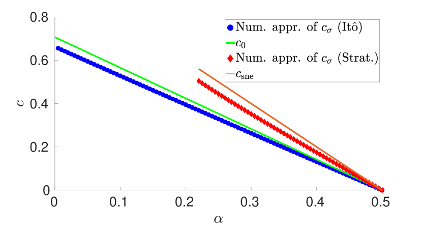
(a)

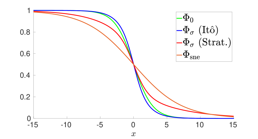
(b)

Figure 3.1: Panel (a) compares the deterministic wave speed (3.6) (green), the instantaneous stochastic wave speed $c_{\sigma}$ for the Ito (blue) and Stratonovich (red) interpretations and the speed $c_{\mathrm{sne}}$ derived in [16, eq. (6.33)] (orange), all for $\sigma=1$ and $\zeta=1$. The red and orange lines are only plotted for $\alpha_{\mathrm{eff}}\in(0,1/2)$. Panel (b) compares the associated wave profiles $\alpha=0.45$ and $\sigma=1.3$. Notice the steepening and flattening of the waves for the Itô respectively Stratonovich interpretations. The profiles are computed on the interval $[-40,40]$, but here zoomed in to $[-15,15]$ to highlight the differences.

In this scalar setting, the full equation $F_{\sigma}(\Phi_{\sigma},c_{\sigma})=0$ can be written as

$$\begin{split}\Phi_{\sigma}^{\prime\prime}+c_{\sigma}\Phi_{\sigma}^{\prime}+f_{\mathrm{cub}}(\Phi_{\sigma})=&-\frac{\sigma^{2}}{2}\frac{\langle q*(g(\Phi_{\sigma})\psi_{\mathrm{tw}}),g(\Phi_{\sigma})\psi_{\mathrm{tw}}\rangle_{L^{2}(\mathbb{R})}}{\langle\Phi_{\sigma}^{\prime},\psi_{\mathrm{tw}}\rangle^{2}_{L^{2}(\mathbb{R})}}\Phi_{\sigma}^{\prime\prime}\\ &+\sigma^{2}\frac{\big{(}g(\Phi_{\sigma})q*(g(\Phi_{\sigma})\psi_{\mathrm{tw}})\big{)}^{\prime}}{\langle\Phi^{\prime}_{\sigma},\psi_{\mathrm{tw}}\rangle_{L^{2}(\mathbb{R})}}-\frac{\mu\sigma^{2}}{2}q(0)g^{\prime}(\Phi_{\sigma})g(\Phi_{\sigma}).\end{split}$$ (3.8)

It is interesting to compare this equation with the system

$$\begin{split}\Phi_{\mathrm{sne}}^{\prime\prime}+c_{\mathrm{sne}}\Phi_{\mathrm{sne}}^{\prime}+f_{\mathrm{cub}}(\Phi_{\mathrm{sne}})=-\frac{\mu\sigma^{2}}{2}q(0)g^{\prime}(\Phi_{\mathrm{sne}})g(\Phi_{\mathrm{sne}})\end{split}$$ (3.9)

used to construct the waves $(\Phi_{\mathrm{sne}},c_{\mathrm{sne}})$ in [16] using their so-called small noise expansion technique. As the authors remark, this equation is not the result of a systematic perturbative expansion in $\sigma$, but rather a partial resummation of such an expansion. For example, the additional two $O(\sigma^{2})$ terms in (3.8) arise from the second order terms in the Itô formula which were neglected in [16].

In any case, for $\mu=1$ we can rewrite (3.9) in the explicit form

$$\Phi_{\mathrm{sne}}^{\prime\prime}+c_{\mathrm{sne}}\Phi_{\mathrm{sne}}^{\prime}+\big{(}1-\sigma^{2}q(0)\big{)}u(1-u)\Big{(}u-\alpha_{\mathrm{eff}}\Big{)}=0,$$ (3.10)

with a new effective detuning parameter

$$\alpha_{\mathrm{eff}}=\frac{2\alpha-\sigma^{2}q(0)}{2-2\sigma^{2}q(0)}.$$ (3.11)

This equation is just a scaled version of the original ODE, which can be solved by rescaling (3.6) as

$$\begin{split}\Phi_{\mathrm{sne}}&=\frac{1}{2}\left[1-\tanh\left(\frac{\sqrt{1-\sigma^{2}q(0)}}{2\sqrt{2}}x\right)\right],\qquad c_{\mathrm{sne}}=\sqrt{2\big{(}1-\sigma^{2}q(0)\big{)}}(\frac{1}{2}-\alpha_{\mathrm{eff}}).\end{split}$$ (3.12)

Our full system (3.8) cannot be solved explicitly, but in the bistable regime $\alpha_{\mathrm{eff}}\in(0,1)$ we were able to use a straightforward numerical boundary value problem solver to approximate the solutions; see Fig. 1(a). These results show that $c_{\mathrm{sne}}$ is a reasonable approximation for $c_{\sigma}$, but in Fig. 4(b) we shall see that $c_{\mathrm{sne}}$ compares less favourably with the full limiting wave speed. Note that our solutions are in agreement with the numerical observations from [34]: for the Stratonovich interpretation the wave moves faster and is less steep, but for the Itô interpretation the wave slows down and becomes steeper.

We now turn to expanding $(\Phi_{\sigma},c_{\sigma})$ in powers of $\sigma$. Following (2.48), the lowest order correction to $c_{\sigma}$ becomes

$$\begin{split}c_{0;2}=&-\frac{1}{2}\langle\Phi_{0}^{\prime\prime},\psi_{\mathrm{tw}}\rangle_{L^{2}(\mathbb{R})}\langle q*(g(\Phi_{0})\psi_{\mathrm{tw}}),g(\Phi_{0})\psi_{\mathrm{tw}}\rangle_{L^{2}(\mathbb{R})}-\langle g(\Phi_{0})q*(g(\Phi_{0})\psi_{\mathrm{tw}}),\psi_{\mathrm{tw}}^{\prime}\rangle_{L^{2}(\mathbb{R})}\\ &\qquad-\frac{\mu q(0)}{2}\langle g^{\prime}(\Phi_{0})g(\Phi_{0}),\psi_{\mathrm{tw}}\rangle_{L^{2}(\mathbb{R})}.\end{split}$$ (3.13)

We can subsequently find $\Phi_{0;2}$ by numerically inverting the linear operator $\mathcal{L}_{\mathrm{tw}}$ to solve

$$\begin{split}\mathcal{L}_{\mathrm{tw}}\Phi_{0;2}&=-\frac{1}{2}\Phi_{0}^{\prime\prime}\langle q*(g(\Phi_{0})\psi_{\mathrm{tw}}),\psi_{\mathrm{tw}}\rangle_{L^{2}(\mathbb{R})}^{2}-c_{0;2}\Phi_{0}^{\prime}+\Big{(}g(\Phi_{0})q*(g(\Phi_{0})\psi_{\mathrm{tw}})\Big{)}^{\prime}\\ &\qquad\qquad-\frac{q(0)}{2}g^{\prime}(\Phi_{0})g(\Phi_{0}).\end{split}$$ (3.14)

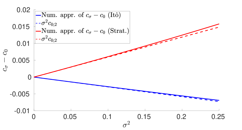
(a)

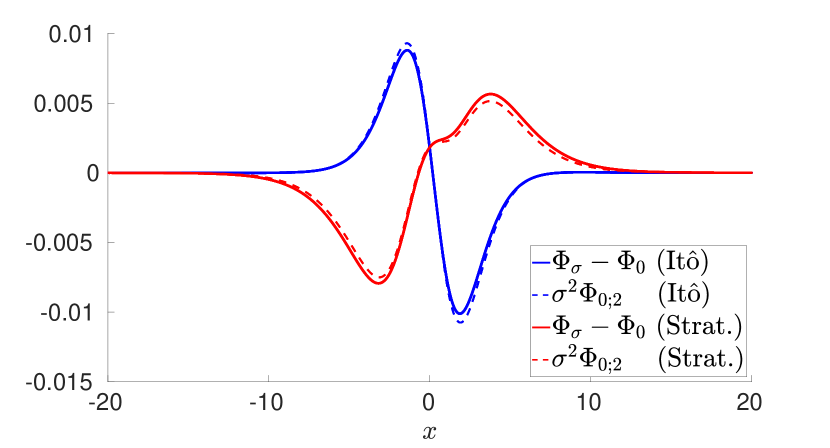
(b)

Figure 3.3: These panels display the stochastic corrections $c_{\sigma}-c_{0}$ and $\Phi_{\sigma}-\Phi_{0}$ for the wave speed (a) and wave profile (b), together with their leading order approximations. We chose $\alpha=0.25$ and $\zeta=1$, which results in $c_{0;2}=-0.0298$ (Itô) and $c_{0;2}=0.0563$ (Stratonovich). The profiles in (b) were computed for $\sigma=0.5$.

We remark that these approximations can also be evaluated for additive noise ($g=1$), or, in the Itô interpretation, for $q(x-y)=\delta(x-y)$. In Fig. 3.3 we compare $(\Phi_{\sigma}-\Phi_{0},c_{\sigma}-c_{0})$ with our quadratic approximations for a range of different values of $\sigma$. There appears to be a good agreement, both for the Itô and Stratonovich interpretation.

Limiting wave speed

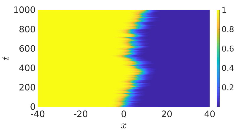
(a) $U(x+c_{0}t,t)$

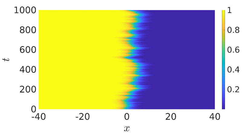
(b) $U(x+c_{\sigma}t,t)$

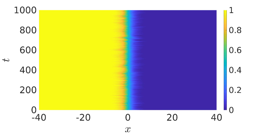
(c) $U(x+\Gamma(t),t)$

Figure 3.2: A single realization of (3.1) in the Stratonovich interpretation with initial condition $\Phi_{\sigma}$ in 3 different reference frames, with parameters $\alpha=0.25$, $\sigma=0.3$ and $\zeta=1$. We can clearly see in (a) that the deterministic speed underestimates the stochastic speed. Replacing $c_{0}$ with $c_{\sigma}$ in (b) captures the movement better, but the position is still fluctuating. Panel (c) shows that these fluctuations can be captured almost completely in the $\Gamma(t)$-frame.

In order to provide some insight on the effectiveness of our stochastic phase $\Gamma(t)$, Fig. 3.2 describes the behaviour of $U(t)$ for a single realization of (3.1) in three different reference frames. The first panel shows the wave in the deterministic co-moving frame, which clearly underestimates the wave speed. Replacing the speed $c_{0}$ by $c_{\sigma}$ gives a better approximation, but the wave is still wandering. The right panel shows that these fluctuations can be largely eliminated by using $\Gamma(t)$, confirming that this an appropriate representation for the position of the wave.

At leading order, the fluctuations around $c_{\sigma}t$ are described by the scaled Brownian motion

$$\Gamma_{0}^{(1)}(t)=\int_{0}^{t}\langle\psi_{\mathrm{tw}},g(\Phi_{0})dW^{Q}_{s}\rangle_{L^{2}(\mathbb{R})}.$$ (3.15)

The corresponding variance is given by

$$\mathrm{Var}\big{(}\sigma\Gamma_{0}^{(1)}(t)\big{)} =\sigma^{2}\langle q*(g(\Phi_{0})\psi_{\mathrm{tw}}),g(\Phi_{0})\psi_{\mathrm{tw}}\rangle_{L^{2}(\mathbb{R})}t,$$ (3.16)

which exactly matches [16, eq. (6.25)]. Since $E\,\Gamma_{0}^{(1)}(t)=0$, the orbital drift corrections to the limiting wave speed are only visible at second order in $\sigma$. In particular, the lowest order contribution given in (2.61) reduces to

$$\begin{split}c_{0;2}^{\mathrm{od}}&=-\frac{1}{2}\int_{0}^{\infty}\sum_{k=0}^{\infty}\langle f_{\mathrm{cub}}^{\prime\prime}(\Phi_{0})\Big{(}S(s)\mathcal{S}_{0}(0)[p*e_{k}]\Big{)}^{2},\psi_{\mathrm{tw}}\rangle_{L^{2}(\mathbb{R})}\,ds.\\ \end{split}$$ (3.17)

Here the square is taken in a pointwise fashion, with

$$\begin{split}\mathcal{S}_{0}(0)[p*e_{k}]&=g(\Phi_{0})p*e_{k}-\Phi^{\prime}_{0}\langle p*e_{k},g(\Phi_{0})\psi_{\mathrm{tw}}\rangle_{L^{2}(\mathbb{R})}.\end{split}$$ (3.18)

In order to evaluate this expression for $c_{0;2}^{\mathrm{od}}$, we need to choose an appropriate orthonormal basis for $L^{2}([-L,L];\mathbb{R})$, where $[-L,L]$ is the domain that we use for the numerical simulations. Following [34, 45], we take

$$e^{(L)}_{k,c}(x)=\frac{1}{\sqrt{L}}\cos(\frac{\pi kx}{L}),\qquad\qquad e^{(L)}_{k,s}(x)=\frac{1}{\sqrt{L}}\sin(\frac{\pi kx}{L})$$ (3.19)

for all integers $k\geq 0$

and introduce the quantities

$$\lambda_{k;\mathrm{apx}}=\mathrm{exp}[-\pi k^{2}\zeta^{2}/L^{2}].$$ (3.20)

A short computation shows that

$$Qe^{(L)}_{k,c}=q*e^{(L)}_{k,c}=\int_{-L}^{L}q(\cdot-y)e^{(L)}_{k,c}(y)dy\approx\int_{-\infty}^{\infty}q(\cdot-y)e^{(L)}_{k,c}(y)dy=\lambda_{k;\mathrm{apx}}e^{(L)}_{k,c}$$ (3.21)

and in the same fashion we find $Qe^{(L)}_{k,s}\approx\lambda_{k;\mathrm{apx}}e^{(L)}_{k,s}$. These observations can be used to approximate the expression (3.17) by writing

$$\begin{split}c^{\mathrm{od}}_{0;2}\approx-\frac{1}{2}\int_{0}^{\infty}\sum_{k=0}^{150}\sum_{\#\in\{c,s\}}\lambda_{k;\mathrm{apx}}\langle f_{\mathrm{cub}}^{\prime\prime}(\Phi_{0})\big{(}S(s)\mathcal{I}^{(L)}_{k\#}\big{)}^{2},\psi_{\mathrm{tw}}\rangle_{L^{2}([-L,L];\mathbb{R})}\,ds,\end{split}$$ (3.22)

in which we have

$$\mathcal{I}^{(L)}_{k\#}=g(\Phi_{0})e^{(L)}_{k\#}-\Phi^{\prime}_{0}\langle e^{(L)}_{k\#},g(\Phi_{0})\psi_{\mathrm{tw}}\rangle_{L^{2}([-L,L];\mathbb{R})}.$$ (3.23)

We verified numerically that the resulting sum converges exponentially fast in both $L$ and $k$.

In order to approximate the cubic coefficient $c^{\mathrm{od}}_{\sigma;3}$, we use the fact that $\Gamma_{\sigma}^{(3)}(t)$ depends only on $V_{\sigma}^{(1)}(t)$ and $V_{\sigma}^{(2)}(t)$. In particular, we made the approximation

$$\sigma^{3}c^{\mathrm{od}}_{0;3}\approx c^{\mathrm{od}}_{\mathrm{cub}}(\sigma)$$ (3.24)

by numerically computing

$$c^{\mathrm{od}}_{\mathrm{cub}}(\sigma)=\frac{2}{T}\int^{T}_{\frac{T}{2}}\frac{1}{t}E\big{[}\Gamma_{\mathrm{apx}}(t)-c_{\sigma}t-\sigma\Gamma_{\sigma}^{(1)}(t)-\sigma^{2}\Gamma_{\sigma}^{(2)}(t)\big{]}\,dt,$$ (3.25)

in which

$$\Gamma_{\mathrm{apx}}(t)=c_{\sigma}t+\int_{0}^{t}a_{\sigma}\big{(}\sigma V_{\sigma}^{(1)}(s)+\sigma^{2}V_{\sigma}^{(2)}(s)\big{)}\,ds+\int_{0}^{t}b_{\sigma}(\sigma V_{\sigma}^{(1)}(s)+\sigma^{2}V_{\sigma}^{(2)}(s)\big{)}\,dW^{Q}_{s}$$ (3.26)

denotes the value for $\Gamma(t)$ that is obtained by integrating (2.20) using only the second order approximation of $V$.

Putting everything together, we obtain the prediction

$$c^{\mathrm{pred}}_{\sigma;\mathrm{lim}}=c_{0}+\sigma^{2}[c_{0;2}+c_{0;2}^{\mathrm{od}}]+c^{\mathrm{od}}_{\mathrm{cub}}(\sigma)+\mathcal{O}(\sigma^{4}).$$ (3.27)

To get a feeling for the sizes of the perturbations in the Stratonovich interpretation, we remark that our computations for $\alpha=0.25$ and $\zeta=1$ yield

$$\begin{split}c^{\mathrm{pred}}_{\sigma;\mathrm{lim}}&=0.3536+\sigma^{2}[0.056-0.0043]+0.0036\sigma^{3}+\mathcal{O}(\sigma^{4}).\end{split}$$ (3.28)

Clearly, the contribution from the orbital drift is significantly smaller then the contribution from $c_{\sigma}$.

To test this prediction, we numerically computed a proxy for the limiting wave speed by evaluating the integral

$$c_{\sigma;\mathrm{lim}}^{\mathrm{obs}}=c_{\sigma}+\frac{2}{T}\int_{\frac{T}{2}}^{T}\frac{1}{t}E[\Gamma(t)-c_{\sigma}t-\sigma\Gamma_{\sigma}^{(1)}(t)]\,dt,$$ (3.29)

which computes the average speed over the interval $[T/2,T]$ in order to remove any transients from the data. Note that subtracting $\Gamma_{\sigma}^{(1)}(t)$ does not change the average but speeds up the convergence towards the average. This computation is motivated by the plots of $E[\Gamma(t)-c_{\sigma}t]$ contained in Fig. 4(a), which have a clear linear trend. This validates the concept of a limiting wavespeed, but also illustrates the need to include the orbital drift corrections to the instantaneous wavespeed $c_{\sigma}$.

In Fig. 4(b) we show the relative deviation of $c_{\sigma;\mathrm{lim}}$ from $c_{0}$, i.e. $(c_{\sigma;\mathrm{lim}}-c_{0})/c_{0}$. The blue dots represent the numerically observed values. The red dashed line shows the quadratic approximation $c_{0}+\sigma^{2}[c_{0;2}+c_{0;2}^{\mathrm{od}}]$ and there is indeed a good correspondence.

We also provide a cubic approximation to the wave speed by adding the term $c^{\mathrm{od}}_{\mathrm{cub}}(\sigma)$. This indeed improves the prediction, validating our computations. However, it also shows that the improvement is small and might not be worth the effort.

For completeness, we also included the predictions (3.9) arising from the small noise expansion technique. The results show that these predictions capture the overall behaviour of the limiting speed correctly, but the values deviate significantly.

(a)

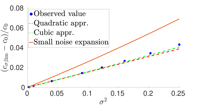
(b)

Figure 3.4: In (a) we computed the average $E[\Gamma(t)-c_{\sigma}t]$ over 1000 simulations of (2.34) for the Stratonovich interpretation, using the procedure described in the main text for several values of $\sigma$. Notice that a clear trend is visible, which validates the orbital drift principle. In (b) we show the relative deviation of $c_{\sigma;\mathrm{lim}}$ from $c_{0}$. Here the observed limiting speed is computed by evaluating the average (3.29) for the data in (a), while the quadratic and cubic approximations were computed using the relevant terms in (3.27). The orange line is the prediction arising from the small noise expansion (3.12). Both plots use $\alpha=0.25$ and $\zeta=1$.

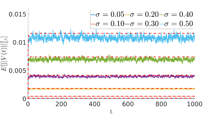
(a)

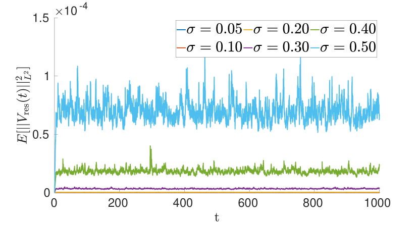
(b)

Figure 3.5: In (a) we computed the average $E[\lVert V(t)\rVert_{L^{2}}^{2}]$ over 1000 realization of (2.34) in the Itô interpretation. The dashed line shows the numerical evaluation of the first order term (3.30). In (b) we computed the corresponding averages for the residual (3.32) by evaluating and subtracting $\sigma V_{\sigma}^{(1)}(t)$ and $\sigma^{2}V_{\sigma}^{(2)}(t)$ for every realization in (a). Note that both $V(t)$ and $V_{\mathrm{res}}(t)$ stabilize over time.

Size of $V(t)$

Next, we turn our attention to the size of the perturbation $V(t)$ defined in (2.34). Although the leading order term $V_{0}^{(1)}(t)$ has zero mean, this does not hold for its norm. Indeed, using (2.70) we find

$$\begin{split}E[\lVert V_{0}^{(1)}(t)\rVert_{L^{2}(\mathbb{R})}^{2}]&=\int_{0}^{t}\lVert S(s)\mathcal{S}_{0}(0)\rVert^{2}_{HS\big{(}L^{2}_{Q},L^{2}(\mathbb{R})\big{)}}ds\\ &=\int_{0}^{t}\sum_{k=0}^{\infty}\lVert S(s)[g(\Phi_{0})p*e_{k}-\Phi^{\prime}_{0}\langle g(\Phi_{0})\psi_{\mathrm{tw}},p*e_{k}\rangle_{L^{2}(\mathbb{R})}]\rVert^{2}_{L^{2}(\mathbb{R})}\,ds.\end{split}$$ (3.30)

This expectation can be approximated using the same basis functions and eigenvalues that we used for the orbital drift. Stated more concretely, we recall (3.23) and write

$$\begin{split}E[\lVert V_{0}^{(1)}(t)\rVert_{L^{2}(\mathbb{R})}^{2}]\approx\int_{0}^{t}\sum_{k=0}^{150}\sum_{\#\in\{c,s\}}\lambda_{k;\mathrm{apx}}\lVert S(s)\mathcal{I}^{(L)}_{k\#}\rVert^{2}_{L^{2}([-L,L];\mathbb{R})}\,ds.\end{split}$$ (3.31)

This function is represented by the red dashed line in Fig. 5(a). This agrees well with the numerical average of $E[\lVert V(t)\rVert_{L^{2}(\mathbb{R})}^{2}]$ that we computed directly from our simulations. The exponential behaviour for short time scales as well as the longer term stabilization are nicely captured by these results. We note that we expect this limiting value to be of order $\mathcal{O}(\sigma^{2})$. This is confirmed by Fig. 7(a), which shows how $E\lVert V(T)\rVert_{L^{2}(\mathbb{R})}^{2}$ scales with $\sigma$ for $T=1000$.

Similar behaviour was found during our simulations for the residual

$$V_{\mathrm{res}}(t)=V(t)-\sigma V_{\sigma}^{(1)}(t)-\sigma^{2}V_{\sigma}^{(2)}(t).$$ (3.32)

Indeed, Fig. 5(b) shows that this residual also stabilizes exponentially fast to a small value which we expect to be $\mathcal{O}(\sigma^{6})$, as confirmed in Fig. 7(a).

We emphasize that we do not expect the running supremum of $\left\|V(t)\right\|_{L^{2}}$ to stabilize in the same fashion. Indeed, we numerically computed $E[\sup_{0\leq s\leq t}\lVert V(s)\rVert^{2}_{L^{2}(\mathbb{R})}]$ for $0\leq t\leq 1000$. The results strongly suggest that this supremum grows logarithmically in time (Fig. 8(a)) and scales as $\sigma^{2}$ for large fixed $t$ (Fig. 8(b)). This is hence significantly better than the $\mathcal{O}(\sigma^{2}t)$ bound that arises from the Burkholder-Davis-Gundy inequality and confirms our belief that our approach can be used to track waves over time scales that are exponential in $\sigma$.

Limiting wave profile

Since $E[V_{\sigma}^{(1)}(t)]=0$, we expect the leading order contribution to the average of $V(t)$ to be given by $\sigma^{2}E[V_{0}^{(2)}(t)]$. Using (3.18) once more, we find that (2.60) can be written as

$$\begin{split}E[V_{0}^{(2)}(t)]=\frac{1}{2}\int_{0}^{t}S(t-s)\int_{0}^{s}\sum_{k=0}^{\infty}\Big{[}&f^{\prime\prime}_{\mathrm{cub}}(\Phi_{0})\left(S(s^{\prime})\mathcal{S}_{0}(0)[p*e_{k}]\right)^{2}\\ &-\Phi^{\prime}_{0}\langle f^{\prime\prime}_{\mathrm{cub}}(\Phi_{0})\left(S(s^{\prime})\mathcal{S}_{0}(0)[p*e_{k}]\right)^{2},\psi_{\mathrm{tw}}\rangle_{L^{2}(\mathbb{R})}\Big{]}ds^{\prime}ds.\end{split}$$ (3.33)

This can be evaluated using the same expressions for the eigenvalues and eigenfunctions that we used for the orbital drift. In order to compare this to our simulations, we numerically approximated $E[V(t)]$ by taking the average over 500 simulations of $V(t)-\sigma V_{\sigma}^{(1)}(t)$. Since $E[V_{\sigma}^{(1)}(t)]=0$, this again speeds up the convergence to the mean. The results are contained in Fig. 3.6, which shows that $\sigma^{2}E[V^{(2)}_{0}(t)]$ is indeed very good approximation for $E[V(t)]$. These plots also show that the average shape indeed appears to converge to a limit, motivating us to write

$$\Phi^{\mathrm{obs}}_{\sigma;\mathrm{lim}}=\Phi_{\sigma}+E[V(20)].$$ (3.34)

We recall our prediction

$$\Phi^{\mathrm{pred}}_{\sigma;\mathrm{lim}}=\Phi_{0}+\sigma^{2}[\Phi_{0;2}+V_{0;2}^{\mathrm{od}}]+O(\sigma^{3})$$ (3.35)

for the limiting wave profile. We can now numerically approximate the expression (2.64) for $V^{\mathrm{od}}_{0;2}$ by computing

$$\begin{split}V^{\mathrm{od}}_{0;2}\approx-\frac{1}{2}\mathcal{L}_{\mathrm{tw}}^{-1}\int_{0}^{T}\sum_{k=0}^{150}\sum_{\#\in\{c,s\}}\lambda_{k;\mathrm{apx}}\Big{[}&f^{\prime\prime}_{\mathrm{cub}}(\Phi_{0})\big{(}S(s)\mathcal{I}^{(L)}_{k\#}\big{)}^{2}\\ &-\Phi^{\prime}_{0}\langle f^{\prime\prime}_{\mathrm{cub}}(\Phi_{0})\big{(}S(s)\mathcal{I}^{(L)}_{k\#}\big{)}^{2},\psi_{\mathrm{tw}}\rangle_{L^{2}([-L,L];\mathbb{R})}\Big{]}\,ds.\end{split}$$ (3.36)

To test our prediction, we compare $\Phi^{\mathrm{obs}}_{\sigma;\mathrm{lim}}-\Phi_{0}$ against $\sigma^{2}[\Phi_{0;2}+V_{0;2}^{\mathrm{od}}]$ for multiple values of $\sigma$. The results are plotted in Fig. 7(b), which again confirms that there is a good match.

(a) $E[V(t)]$

(b) $\sigma^{2}E[V_{0}^{(2)}(t)]$

Figure 3.6: Panel (a) displays the average of $V(t)$ over 500 iterations of (3.1) in the Stratonovich interpretation for $\alpha=0.25$, $\zeta=1$ and $\sigma=0.5$. Panel (b) contains a numerical evaluation of (3.33) that includes the first 150 terms of the sum.

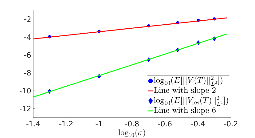
(a)

(b)

Figure 3.7: The datapoints in (a) are computed from Fig. 3.5 by evaluating the expectations at $T=1000$ and plotting them as function of $\sigma$. We observe that $E[\lVert V(T)\rVert_{L^{2}(\mathbb{R})}^{2}]$ and $E[\lVert V_{\mathrm{res}}(T)\rVert_{L^{2}(\mathbb{R})}^{2}]$ scale as $\mathcal{O}(\sigma^{2})$ and $\mathcal{O}(\sigma^{6})$ respectively, as predicted. Panel (b) compares the observed (solid) and predicted (dashed) limiting deviations from $\Phi_{0}$ for multiple values of $\sigma$ in the Stratonovich interpretation, see (3.34) and (3.35).

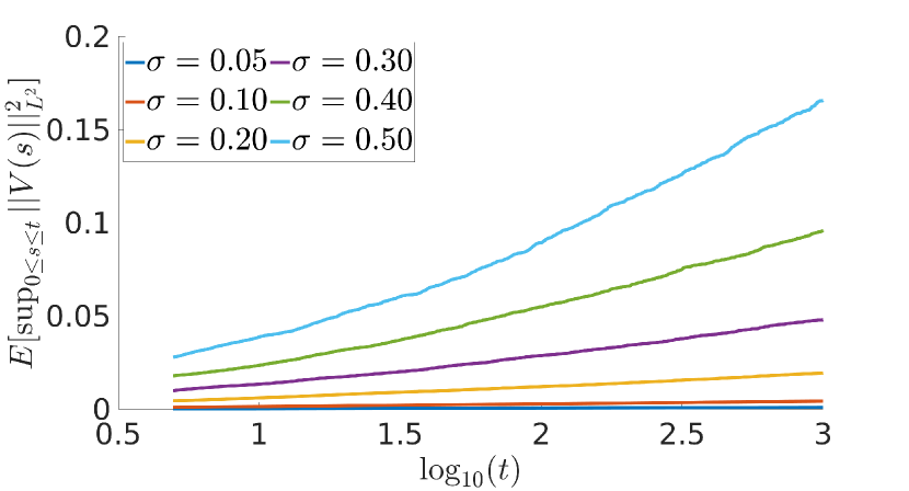
(a)

(b)

Figure 3.8: Panel (a) shows the numerical evaluation of $E[\sup_{0\leq s\leq t}\lVert V(s)\rVert^{2}_{L^{2}(\mathbb{R})}]$ for different values of $\sigma$, where the average is computed over 500 iterations. The trend lines indicate that this supremum admits logarithmic growth. Panel (b) plots the supremum at $t=1000$ against $\sigma$, illustrating the $\mathcal{O}(\sigma^{2})$ behaviour. We used the Itô interpretation with $\alpha=0.25$ and $\zeta=1$.

4 Example II: The FitzHugh-Nagumo system

In this section we repeat the experiments from §3 for the two-component FitzHugh-Nagumo system

$$\begin{split}dU&=\big{[}U_{xx}+f_{\mathrm{cub}}(U)-W+\mu\sigma^{2}h^{(u)}(U,W)]dt+\sigma g^{(u)}(U,W)dW^{Q_{1}}_{t},\\[5.69046pt] dW&=\big{[}\varrho V_{xx}+\varepsilon(U-\gamma W)+\mu\sigma^{2}h^{(w)}(U,W)]dt+\sigma g^{(w)}(U,W)dW^{Q_{2}}_{t},\end{split}$$ (4.1)

where $f_{\mathrm{cub}}$ is the same cubic polynomial as in §3 and $\varrho,\varepsilon,\gamma,\sigma>0$. We assume that the two processes $W^{Q_{1}}_{t}$ and $W^{Q_{2}}_{t}$ are independent, allowing us to write

$$g(U,W)=\begin{pmatrix}g^{(u)}(U,W)&0\\ 0&g^{(w)}(U,W)\end{pmatrix},\hskip 28.45274ptQ\begin{pmatrix}v_{1}\\ v_{2}\end{pmatrix}=\begin{pmatrix}Q_{1}v_{1}&0\\ 0&Q_{2}v_{2}\end{pmatrix}=\begin{pmatrix}q_{1}*v_{1}&0\\ 0&q_{2}*v_{2}\end{pmatrix}$$ (4.2)

for two convolution kernels $q_{1}$ and $q_{2}$. In particular, we have $n=m=2$ and we assume that the combination $\mathrm{diag}(q_{1},q_{2})$ satisfies (Hq).

Upon combining the general computations in [14, p. 123] with the abstract infinite-dimensional framework developed in [47, §4.1], one can show that the Itô-Stratonovich correction term is given by

$$\big{(}h^{(u)}(U,W),h^{(w)}(U,W)\big{)}^{T}=\frac{1}{2}\Big{(}q_{1}(0)D_{1}g^{(u)}(U,W)g^{(u)}(U,W),q_{2}(0)D_{2}g^{(w)}(U,W)g^{(w)}(U,W)\Big{)}^{T}.$$ (4.3)

As usual, we can switch between the Itô $(\mu=0)$ and Stratonovich ($\mu=1$) interpretations for the noise term.

All the expressions that we derive in this section are valid for the general situation described in (4.2). However, in order to generate our plots we used the specific choices

$$g^{(u)}(U,W)=U,\qquad g^{(w)}(U,W)=0,\qquad q_{1}(x)=q_{2}(x)=\frac{1}{2}e^{\frac{-\pi x^{2}}{4}},$$ (4.4)

together with the parameter values $\alpha=0.1$, $\varrho=0.01$, $\varepsilon=0.01$ and $\gamma=5$. Although we were unable to find prior work to which our results can be compared, we do point out that computations for the somewhat related Barkley model are discussed in [15].

(a)

(b)

Figure 4.1: These panels display the stochastic corrections $c_{\sigma}-c_{0}$ for the wave speed (a) and the stochastic wave profiles $\Phi_{\sigma}$ for $\sigma=0.3$ (b), together with their quartic approximations.

Computing $(\Phi_{\sigma},c_{\sigma})$.

Assume for the moment that the deterministic travelling wave ODE

$$\begin{split}\partial_{\xi\xi}\Phi^{(u)}_{0}+c_{0}\partial_{\xi}\Phi^{(u)}_{0}+f_{\mathrm{cub}}(\Phi_{0}^{(u)})-\Phi^{(w)}_{0}=&\,0,\\ \varrho\partial_{\xi\xi}\Phi^{(w)}_{0}+c_{0}\partial_{\xi}\Phi^{(w)}_{0}+\varepsilon(\Phi^{(u)}_{0}-\gamma\Phi^{(w)}_{0})=&\,0\end{split}$$ (4.5)

has a spectrally stable wave solution $\Phi_{0}=(\Phi^{(u)}_{0},\Phi^{(w)}_{0})$. We then recall the associated linear operator $\mathcal{L}_{\mathrm{tw}}:H^{2}(\mathbb{R},\mathbb{R}^{2})\to L^{2}(\mathbb{R},\mathbb{R}^{2})$ that acts as

$$\begin{array}[]{lcl}\mathcal{L}_{\mathrm{tw}}&=&\left(\begin{array}[]{cc}\partial_{\xi\xi}+c_{0}\partial_{\xi}+f^{\prime}_{\mathrm{cub}}(\Phi_{0}^{(u)})&-1\\[5.69046pt] \varepsilon&\varrho\partial_{\xi\xi}+c_{0}\partial_{\xi}-\varepsilon\gamma\\[5.69046pt] \end{array}\right),\end{array}$$ (4.6)

together with the formal adjoint operator that is given by

$$\begin{array}[]{lcl}\mathcal{L}^{*}_{\mathrm{tw}}&=&\left(\begin{array}[]{cc}\partial_{\xi\xi}-c_{0}\partial_{\xi}+f^{\prime}_{\mathrm{cub}}(\Phi_{0}^{(u)})&\varepsilon\\[5.69046pt] -1&\varrho\partial_{\xi\xi}-c_{0}\partial_{\xi}-\varepsilon\gamma\\[5.69046pt] \end{array}\right).\end{array}$$ (4.7)

The spectral stability implies that $\mathcal{L}^{*}_{\mathrm{tw}}$ admits an eigenfunction $\psi_{\mathrm{tw}}=(\psi^{(u)}_{\mathrm{tw}},\psi^{(w)}_{\mathrm{tw}})$ that can be normalized in such a way that

$$\langle\partial_{\xi}\Phi_{0},\psi_{\mathrm{tw}}\rangle_{L^{2}(\mathbb{R},\mathbb{R}^{2})}=1.$$ (4.8)

To summarize, we have

$$\mathcal{L}_{\mathrm{tw}}\partial_{\xi}(\Phi^{(u)}_{0},\Phi^{(w)}_{0})^{T}=0,\qquad\qquad\mathcal{L}^{*}_{\mathrm{tw}}(\psi^{(u)}_{\mathrm{tw}},\psi^{(w)}_{\mathrm{tw}})^{T}=0.$$ (4.9)

The existence of such spectrally stable waves has been obtained in various parameter regions [1, 9, 10, 23], but no explicit expressions are available for $(\Phi_{0},c_{0})$. However, they can readily be computed numerically.

Upon writing $\Phi_{\sigma}=(\Phi^{(u)}_{\sigma},\Phi^{(w)}_{\sigma})$, the stochastic wave equation $F_{\sigma}(\Phi_{\sigma},c_{\sigma})=0$ becomes

$$\begin{split}\partial_{\xi\xi}\Phi^{(u)}_{\sigma}+c_{\sigma}\partial_{\xi}\Phi^{(u)}_{\sigma}+f_{\mathrm{cub}}(\Phi_{\sigma}^{(u)})-\Phi^{(w)}_{\sigma}=&-\frac{\sigma^{2}}{2}\tilde{b}(\Phi_{\sigma})\partial_{\xi\xi}\Phi^{(u)}_{\sigma}-\mu\sigma^{2}h^{(u)}(\Phi_{\sigma})\\ &\qquad+\sigma^{2}\frac{\partial_{\xi}[g^{(u)}(\Phi_{\sigma})q_{1}*(g^{(u)}(\Phi_{\sigma})\psi^{(u)}_{\mathrm{tw}})]}{\langle\partial_{\xi}\Phi_{\sigma},\psi_{\mathrm{tw}}\rangle_{L^{2}(\mathbb{R},\mathbb{R}^{2})}},\\ \varrho\partial_{\xi\xi}\Phi^{(w)}_{\sigma}+c_{\sigma}\partial_{\xi}\Phi^{(w)}_{\sigma}+\varepsilon(\Phi^{(u)}_{\sigma}-\gamma\Phi^{(w)}_{\sigma})=&-\frac{\sigma^{2}}{2}\tilde{b}(\Phi_{\sigma})\partial_{\xi\xi}\Phi^{(w)}_{\sigma}-\mu\sigma^{2}h^{(w)}(\Phi_{\sigma})\\ &\qquad+\sigma^{2}\frac{\partial_{\xi}[g^{(w)}(\Phi_{\sigma})q_{2}*(g^{(w)}(\Phi_{\sigma})\psi^{(w)}_{\mathrm{tw}})]}{\langle\partial_{\xi}\Phi_{\sigma},\psi_{\mathrm{tw}}\rangle_{L^{2}(\mathbb{R},\mathbb{R}^{2})}},\end{split}$$ (4.10)

where $\tilde{b}$ is given by

$$\tilde{b}(\Phi)=-\frac{\langle q_{1}*(g^{(u)}(\Phi)\psi^{(u)}_{\mathrm{tw}}),g^{(u)}(\Phi)\psi^{(u)}_{\mathrm{tw}}\rangle_{L^{2}(\mathbb{R})}+\langle q_{2}*(g^{(w)}(\Phi)\psi^{(w)}_{\mathrm{tw}}),g^{(w)}(\Phi)\psi^{(w)}_{\mathrm{tw}}\rangle_{L^{2}(\mathbb{R})}}{\langle\partial_{\xi}\Phi_{\sigma},\psi_{\mathrm{tw}}\rangle_{L^{2}(\mathbb{R},\mathbb{R}^{2})^{2}}}.$$ (4.11)

Using (4.10) to evaluate (2.48), we find that the lowest order correction to the speed $c_{\sigma}$ reduces to

$$\begin{split}c_{0;2}=&-\frac{1}{2}\tilde{b}(\Phi_{0})\langle\partial_{\xi\xi}\Phi_{0},\psi_{\mathrm{tw}}\rangle_{L^{2}(\mathbb{R},\mathbb{R}^{2})}-\langle g^{(u)}(\Phi_{0})q_{1}*(g^{(u)}(\Phi_{0})\psi^{(u)}_{\mathrm{tw}}),\partial_{\xi}\psi^{(u)}_{\mathrm{tw}}\rangle_{L^{2}(\mathbb{R})}\\ &\qquad-\langle g^{(w)}(\Phi_{0})q_{2}*(g^{(w)}(\Phi_{0})\psi^{(w)}_{\mathrm{tw}}),\partial_{\xi}\psi^{(w)}_{\mathrm{tw}}\rangle_{L^{2}(\mathbb{R})}-\mu\langle h(\Phi_{0}),\psi_{\mathrm{tw}}\rangle_{L^{2}(\mathbb{R},\mathbb{R}^{2})}.\end{split}$$ (4.12)

In Fig. 1(a) we numerically computed $c_{\sigma}$ for the two interpretations. It turns out that the second order approximation above is only accurate for a range of $\sigma$ that is much smaller than we saw for the Nagumo equation. By also including the quartic term $c_{0;4}$ in our expansion we are able to track $\Phi_{\sigma}$ reasonably well up to $\sigma=0.3$. This is more than sufficient for practical purposes, as our simulations of the full system (4.1) revealed that the pulse is unstable for values of $\sigma$ larger than approximately $\sigma=0.15$.

Fig. 1(b) displays the shape of the instantaneous stochastic wave profile $\Phi_{\sigma}$ for the two different interpretations. It is striking that the wave becomes significantly wider for Stratonovich noise.

(a) $U(x+c_{0}t,t)$

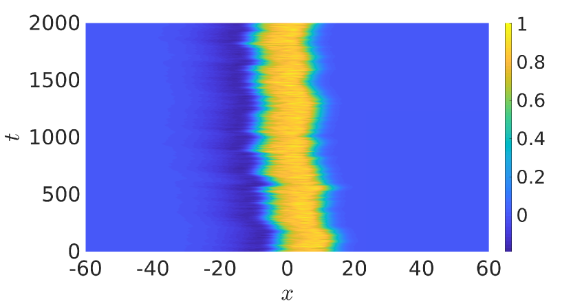
(b) $U(x+c_{\sigma}t,t)$

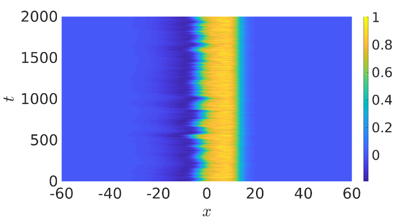
(c) $U(x+\Gamma(t),t)$

Figure 4.2: A single realization of the $U$-component of (4.1) with $\sigma=0.1$ in 3 different reference frames. The initial condition is given by $U(0)=\Phi_{\sigma}$.

Limiting wave speed

In Fig. 4.2 we illustrate the behaviour of a representative sample solution to (4.1) by plotting it in three different moving frames. Fig. 2(a) clearly shows that the deterministic speed $c_{0}$ overestimates the actual speed as the wave moves to the left. The situation is slightly improved in Fig. 2(b), where we use a frame that travels with the stochastic speed $c_{\sigma}$. However, the position of the wave now fluctuates around a position that still moves slowly to the left as a consequence of the orbital drift. This is remedied in Fig. 2(c), where we use the full stochastic phase $\Gamma(t)$. This again validates the idea of using $\Gamma(t)$ as position of the wave.

As in the previous example, the variance of $\Gamma(t)$ is well-described by the variance of the leading order term $\Gamma_{0}^{(1)}$, which is given by

$$\begin{split}\mathrm{Var}\big{(}\Gamma_{0}^{(1)}(t)\big{)}&=\langle q_{1}*(g^{(u)}(\Phi_{0})\psi_{\mathrm{tw}}^{(u)}),g^{(u)}(\Phi_{0})\psi_{\mathrm{tw}}^{(u)}\rangle_{L^{2}(\mathbb{R})}t\\ &\qquad+\langle q_{2}*(g^{(w)}(\Phi_{0})\psi_{\mathrm{tw}}^{(w)}),g^{(w)}(\Phi_{0})\psi_{\mathrm{tw}}^{(w)}\rangle_{L^{2}(\mathbb{R})}t.\end{split}$$ (4.13)

In order to explain the drift observed in Fig. 4.2, we split the semigroup $S(t)$ into its two rows by writing $S(t)=\big{(}S^{(u)}(t),S^{(w)}(t)\big{)}^{T}$. The coefficient (2.61) can now be computed as

$$\begin{split}c^{\mathrm{od}}_{0;2}=\lim_{t\to\infty}t^{-1}E[\Gamma_{0}^{(2)}(t)]&=-\int_{0}^{\infty}\sum_{k=0}^{\infty}\langle K_{0}(s)[\sqrt{Q}e_{k},\sqrt{Q}e_{k}],\psi_{\mathrm{tw}}\rangle_{L^{2}(\mathbb{R},\mathbb{R}^{2})}ds\\ &=-\frac{1}{2}\int_{0}^{\infty}\sum_{k=0}^{\infty}\langle f^{\prime\prime}_{\mathrm{cub}}(\Phi_{0}^{(u)})\big{(}S^{(u)}(s)\mathcal{I}_{k}\big{)}^{2},\psi^{(u)}_{\mathrm{tw}}\rangle_{L^{2}(\mathbb{R})}\,ds.\end{split}$$ (4.14)

Here $\mathcal{I}_{k}$ is given by

$$\mathcal{I}_{k} =\begin{pmatrix}g^{(u)}(\Phi_{0})p_{1}*e^{(u)}_{k}\\ g^{(w)}(\Phi_{0})p_{2}*e^{(w)}_{k}\end{pmatrix}-\alpha_{k}\partial_{\xi}\begin{pmatrix}\Phi_{0}^{(u)}\\ \Phi_{0}^{(w)}\end{pmatrix},$$ (4.15)

in which $(e_{k})=(e_{k}^{(u)},e_{k}^{(w)})$ is a basis of $L^{2}(\mathbb{R},\mathbb{R}^{2})$ and $\alpha_{k}$ is given by

$$\alpha_{k}=\frac{\langle p_{1}*e^{(u)}_{k},g^{(u)}(\Phi_{0})\psi^{(u)}_{\mathrm{tw}}\rangle_{L^{2}(\mathbb{R})}+\langle p_{2}*e^{(w)}_{k},g^{(w)}(\Phi_{0})\psi^{(w)}_{\mathrm{tw}}\rangle_{L^{2}(\mathbb{R})}}{\langle\partial_{\xi}\Phi_{0},\psi_{\mathrm{tw}}\rangle_{L^{2}(\mathbb{R},\mathbb{R}^{2})}}.$$ (4.16)

It is important to note here that the two components in the equation above mix even when $g^{(w)}=0$ due to the presence of the semigroup.

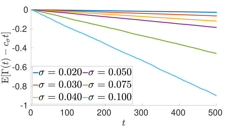
(a)

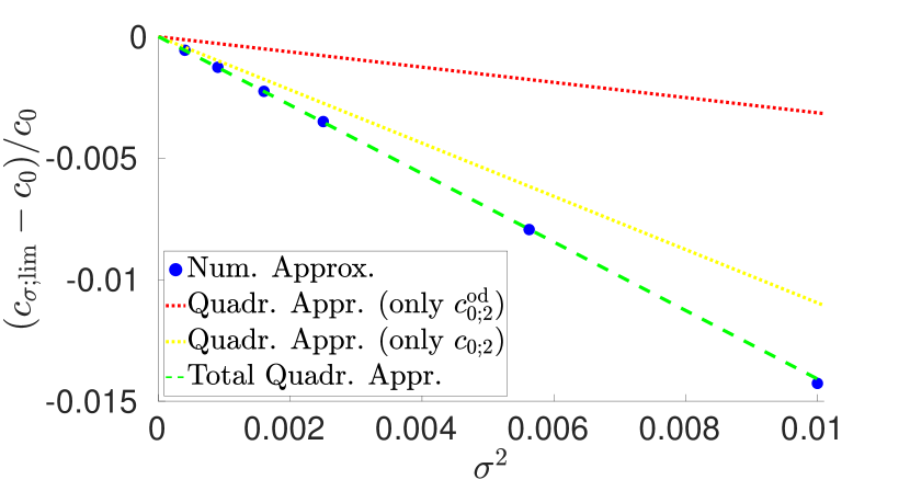
(b)

Figure 4.3: In (a) we computed the average $E[\Gamma(t)-c_{\sigma}t]$ over 500 simulations of (2.34) with $\mu=0$ for several values of $\sigma$, using the procedure described in the main text. Notice that a clear trend is visible. In (b) we show the relative deviation of $c_{\sigma;\mathrm{lim}}$ from $c_{0}$. Here the observed limiting speed is computed by evaluating the average (4.18) for the data in (a), while the various quadratic predictions are obtained from the relevant terms in (4.17).

In order to evaluate (4.14) numerically, we reuse the basis (3.19) for $L^{2}([-L,L];\mathbb{R})$ to construct a basis for $L^{2}([-L,L];\mathbb{R})\times L^{2}([-L,L];\mathbb{R})$. Because $Q$ is diagonal we can also recycle the approximate eigenvalues $\lambda_{k;\mathrm{apx}}$. For the Itô interpretation and the parameter values used in Fig. 3(a), we obtain

$$\begin{split}c^{\mathrm{pred}}_{\sigma;\mathrm{lim}}&=c_{0}+\sigma^{2}[c_{0;2}+c^{\mathrm{od}}_{0;2}]+\mathcal{O}(\sigma^{3})\\ &=0.4693-\sigma^{2}[0.5138+0.1470]+\mathcal{O}(\sigma^{3}).\end{split}$$ (4.17)

Clearly, for the FitzHugh-Nagumo equation the influence of the orbital drift is significant.

To validate our predictions, we again numerically compute

$$c_{\sigma;\mathrm{lim}}^{\mathrm{obs}}=c_{\sigma}+\frac{2}{T}\int_{\frac{T}{2}}^{T}\frac{1}{t}E[\Gamma(t)-c_{\sigma}t-\sigma\Gamma_{\sigma}^{(1)}(t)]\,dt$$ (4.18)

and compare the outcome with (4.17). Fig. 3(b) shows that the total observed speed is indeed well approximated by the two leading order corrections, $\sigma^{2}c_{0;2}$ and $\sigma^{2}c_{0;2}^{\mathrm{od}}$.

Size of $V(t)$

We now turn our attention to the perturbation

$$V(t)=(V^{(u)}(t),V^{(w)}(t))=\big{(}U(\cdot+\Gamma(t),t),W(\cdot+\Gamma(t),t)\big{)}-(\Phi_{\sigma}^{(u)},\Phi_{\sigma}^{(w)})$$ (4.19)

introduced in (2.34). As in §3, Figs. 4(a) and 6(a) show that $E\lVert V(t)\rVert_{L^{2}(\mathbb{R},\mathbb{R}^{2})}^{2}$ stabilizes exponentially fast to a fixed value of size $O(\sigma^{2})$. These curves are nicely captured by the red dashed lines, which describe the integral

$$\begin{split}E[\lVert V_{0}^{(1)}(t)\rVert_{L^{2}(\mathbb{R},\mathbb{R}^{2})}^{2}]&=\int_{0}^{t}\sum_{k=0}^{\infty}\lVert S(s)\mathcal{I}_{k}\rVert^{2}_{L^{2}(\mathbb{R},\mathbb{R}^{2})}ds\end{split}$$ (4.20)

that measure the size of the first order approximation

$$V_{0}^{(1)}(t)=\big{(}V_{0}^{(u,1)}(t),V_{0}^{(w,1)}(t)\big{)}^{T}.$$ (4.21)

Fig. 4(b) shows that $E\lVert V_{\mathrm{res}}(t)\rVert^{2}_{L^{2}(\mathbb{R},\mathbb{R}^{2})}$ also stabilizes over time, but Fig. 6(a) indicates that the expected $\mathcal{O}(\sigma^{6})$ scaling is not achieved (although the behaviour is significantly better than $\mathcal{O}(\sigma^{4})$). We expect that this can be improved by utilizing more advanced numerical schemes, but do not pursue this further here.

Limiting Wave Profile

Turning our attention to the average shape of $V(t)$, we recall (4.15) and note that (2.60) can be computed as

$$\begin{split}E\,[V_{0}^{(2)}(t)]=&\frac{1}{2}\int_{0}^{t}S(t-s)\int_{0}^{s}\sum_{k=0}^{\infty}\Big{[}\begin{pmatrix}f_{\mathrm{cub}}^{\prime\prime}(\Phi_{0})\big{(}S^{(u)}(s^{\prime})\mathcal{I}_{k}\big{)}^{2}\\ 0\end{pmatrix}\\ &\qquad\qquad-\Phi^{\prime}_{0}\langle f_{\mathrm{cub}}^{\prime\prime}(\Phi_{0})\big{(}S^{(u)}(s^{\prime})\mathcal{I}_{k}\big{)}^{2},\psi^{(u)}_{\mathrm{tw}}\rangle_{L^{2}(\mathbb{R})}\Big{]}\,ds^{\prime}ds.\end{split}$$ (4.22)

In Fig. 4.5 we compare this second-order expression with the numerical average of $E[V(t)]$ over 500 simulations of (4.1). To speed up the convergence of the average, we subtract both $\sigma V_{\sigma}^{(1)}(t)$ and the stochastic integral of $\sigma^{2}V_{\sigma}^{(2)}(t)$ from $V(t)$. This does not change the outcome as both terms have zero expectation.

Notice that these two processes are almost indistinguishable from each other. To illustrate this, we provide snapshots of both processes at $t=50$ in Fig. 6(b) for various values of $\sigma$. Notice that the second-order approximants follow the intricate shape of $E[V(t)]$ very closely.

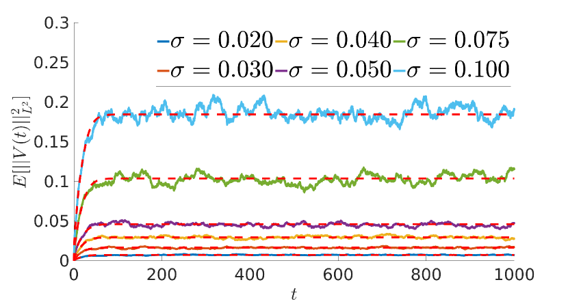
(a)

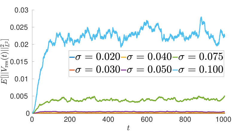
(b)

Figure 4.4: In (a) we computed the average $E[\lVert V(t)\rVert_{L^{2}}^{2}]$ over 500 realization of (2.34) in the Itô interpretation. The dashed line shows the numerical evaluation of the first order term (4.20). In (b) we computed the corresponding averages for the residual (3.32) by evaluating and subtracting $\sigma V_{\sigma}^{(1)}(t)$ and $\sigma^{2}V_{\sigma}^{(2)}(t)$ for every realization in (a). Again, both $V(t)$ and $V_{\mathrm{res}}(t)$ stabilize over time.

(a) $E[V^{(u)}(t)]$

(b) $\sigma^{2}E[V_{0}^{(u,2)}(t)]$

Figure 4.5: Panel (a) shows the average of the first component of $V(t)$, computed over 500 iterations of (4.1) with $\sigma=0.1$ and $\mu=0$. Panel (b) shows the first component of the numerical evaluation of (4.22). As before, there is a good correspondence between the two figures.

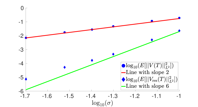
(a)

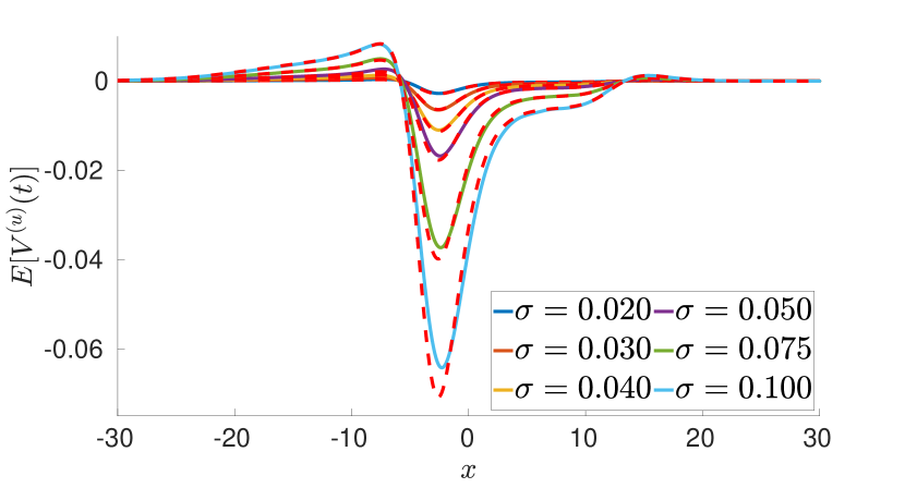
(b)

Figure 4.6: Panel (a) is computed from Fig. 4.4 by evaluating the expectations at the last time step $T=1000$ and plotting them as function of $\sigma$. We observe that $E[\lVert V(T)\rVert_{L^{2}(\mathbb{R},\mathbb{R}^{2})}^{2}]$ scales as $\mathcal{O}(\sigma^{2})$ as predicted and $E[\lVert V_{\mathrm{res}}(T)\rVert_{L^{2}(\mathbb{R},\mathbb{R}^{2})}^{2}]$ scales significantly faster then $\mathcal{O}(\sigma^{4})$, but not as the predicted $\mathcal{O}(\sigma^{6})$. Panel (b) is computed from Fig. 4.5, by evaluating $E[V^{(u)}(50)]$. The dashed lines correspond to the second order predictions $\sigma^{2}E[V_{0}^{(u,2)}(50)]$.

5 The stochastic phase-shift

In this section we derive the SPDE (2.34) that we used to describe the behaviour of the phase-shifted perturbation

$$V(t)=T_{-\Gamma(t)}[X(t)+\Phi_{\mathrm{ref}}]-\Phi_{\sigma}$$ (5.1)

introduced in (2.21). Here $T_{\gamma}$ stands for the right-shift operator $T_{\gamma}U=U(\cdot-\gamma)$. We recall from §2 that the process $X$ is a solution to the SPDE

$$\begin{split}dX&=\big{[}\rho\partial_{xx}(X+\Phi_{\mathrm{ref}})+f(X+\Phi_{\mathrm{ref}})+\sigma^{2}h(X+\Phi_{\mathrm{ref}})\big{]}dt+\sigma g(X+\Phi_{\mathrm{ref}})dW^{Q}_{t}\\ \end{split}$$ (5.2)

posed on the Hilbert space $L^{2}(\mathbb{R},\mathbb{R}^{n})$. In addition, the phase $\Gamma(t)$ was assumed to satisfy the SODE

$$d\Gamma=\big{[}c_{\sigma}+\overline{a}_{\sigma}(U,\Gamma)\big{]}\,dt+\sigma\overline{b}(U,\Gamma)dW^{Q}_{t},$$ (5.3)

with nonlinearities $\overline{a}_{\sigma}$ and $\overline{b}$ that were only defined locally.

In §5.1 we sketch how the noise process $dW^{Q}_{t}$ can be rigorously constructed. We subsequently introduce several cut-off functions in §5.2 that allow us to define $\overline{a}_{\sigma}$ and $\overline{b}$ in such a way that (5.3) remains well-posed globally. This allows us to formulate an appropriate Itô lemma in §5.3, which we use in §5.4 to perform the computations that lead to (2.34).

5.1 Background

In this section we briefly recall some of the functional analysis needed to set up the rigorous framework to study SPDEs. In order to ease the comparison with the earlier work in [20], it turns out to be convenient to work in an abstract setting for the moment. In particular, we consider noise that lives in an arbitrary separable Hilbert space $\mathcal{W}$ and pick a non-negative symmetric operator $Q\in\mathcal{L}(\mathcal{W},\mathcal{W})$. We then write

$$\mathcal{W}_{Q}=Q^{1/2}(\mathcal{W}),$$ (5.4)

which is again a separable Hilbert space with inner product

$$\langle v,w\rangle_{\mathcal{W}_{Q}}=\langle Q^{-1/2}v,Q^{-1/2}v\rangle_{\mathcal{W}}.$$ (5.5)

We now fix an orthonormal basis $(e_{k})$ for $\mathcal{W}$, which means that $(\sqrt{Q}e_{k})$ is a basis for $\mathcal{W}_{Q}$. For any Hilbert space $\mathcal{H}$, we recall that a linear map $\Lambda:\mathcal{W}_{Q}\to\mathcal{H}$ is contained in the set of Hilbert-Schmidt operators $HS(\mathcal{W}_{Q},\mathcal{H})$ if it satisfies $\langle\Lambda,\Lambda\rangle_{HS(\mathcal{W}_{Q},\mathcal{H})}<\infty$. Here the inner product is given by

$$\begin{split}\langle\Lambda_{1},\Lambda_{2}\rangle_{HS(\mathcal{W}_{Q},\mathcal{H})}:&=\sum_{k=0}^{\infty}\langle\Lambda_{1}\sqrt{Q}{e}_{k},\Lambda_{2}\sqrt{Q}{e}_{k}\rangle_{\mathcal{H}}.\end{split}$$ (5.6)

The construction in [42, §2.5] allow us to define a Hilbert space $\mathcal{W}_{\mathrm{ext}}\supset\mathcal{W}$ so that the inclusion $\mathcal{W}_{Q}\subset\mathcal{W}_{\mathrm{ext}}$ is such a Hilbert-Schmidt operator. This (non-unique) extension space is the key ingredient that allows our noise process to be rigorously constructed.

Turning to this task, we introduce a complete probability space $\Big{(}\Omega,\mathcal{F},\mathbb{P}\Big{)}$, together with a normal filtration $(\mathcal{F}_{t})_{t\geq 0}$ and a set of independent $(\mathcal{F}_{t})$-Brownian motions $(\beta_{k})$. Following [28, Eq. (2)], we introduce the formal sum

$$W^{Q}_{t}=\sum_{k=0}^{\infty}\sqrt{Q}e_{k}\beta_{k}(t),$$ (5.7)

which converges in $L^{2}(\Omega,\mathcal{F},P;\mathcal{W}_{\mathrm{ext}})$ for every $t\geq 0$. We will refer to this limiting process $W^{Q}_{t}$ as a $(\mathcal{F}_{t},Q)$-cylindrical Wiener process. The computations in [28, Prop. 2] show that the formal sums

$$\langle W^{Q}_{t},w\rangle_{\mathcal{W}}=\sum_{k=0}^{\infty}\langle\sqrt{Q}e_{k},w\rangle_{\mathcal{W}}\,\beta_{k}(t),\qquad\qquad w\in\mathcal{W}$$ (5.8)

define scalar Wiener processes that satisfy

$$E\Big{[}\langle W^{Q}_{t},w_{1}\rangle_{\mathcal{W}}\langle W^{Q}_{s},w_{2}\rangle_{\mathcal{W}}\Big{]}=(t\wedge s)\langle Qw_{1},w_{2}\rangle_{\mathcal{W}}.$$ (5.9)

For any Hilbert space $\mathcal{H}$ and any $T>0$, we follow the convention in [42, 43] and introduce the space

$$\begin{array}[]{lcl}\mathcal{N}^{2}\big{(}[0,T];(\mathcal{F}_{t});\mathcal{H}\big{)}&=&\{X\in L^{2}\big{(}[0,T]\times\Omega;dt\otimes\mathbb{P};\mathcal{H}\big{)}:\\[5.69046pt] &&\qquad\qquad X\hbox{ has a }(\mathcal{F}_{t})\hbox{-progressively measurable version}\}.\end{array}$$ (5.10)

For any process $B\in\mathcal{N}^{2}\big{(}[0,T];(\mathcal{F}_{t});HS(\mathcal{W}_{Q},\mathcal{H})\big{)}$, we now use [28, Eq (7)] to define the stochastic integral

$$\int_{0}^{t}B(s)\,dW^{Q}_{s}=\lim_{m\to\infty}\sum_{k=0}^{m}\int_{0}^{t}B(s)[\sqrt{Q}e_{k}]\,d\beta_{k}(s)$$ (5.11)

for all $0\leq t\leq T$. This limit can be taken directly in $L^{2}(\Omega,\mathcal{F},P;\mathcal{H})$ and hence avoids the use of the external space. In this setting, the Itô isometry can be stated as

$$E\langle\int_{0}^{t}B_{1}(s)\,dW^{Q}_{s},\int_{0}^{t}B_{2}(s)\,dW^{Q}_{s}\rangle_{\mathcal{H}}=E\,\int_{0}^{t}\langle B_{1}(s),B_{2}(s)\rangle_{HS(\mathcal{W}_{Q},\mathcal{H})}\,ds.$$ (5.12)

Returning to our main SPDE (2.4), we assume for the moment that $g(U)$ is a Hilbert-Schmidt operator from $\mathcal{W}_{Q}$ into $L^{2}(\mathbb{R},\mathbb{R}^{n})$ for every $U\in\mathcal{U}_{H^{1}}$. The formal adjoint

$$g^{\mathrm{adj}}(U):L^{2}(\mathbb{R},\mathbb{R}^{n})\to\mathcal{W}_{Q}$$ (5.13)

is then defined in such a way that

$$\langle g(U)[w],\psi\rangle_{L^{2}(\mathbb{R},\mathbb{R}^{n})}=\langle w,g^{\mathrm{adj}}(U)\psi\rangle_{\mathcal{W}_{Q}}=\langle Q^{-1/2}w,Q^{-1/2}g^{\mathrm{adj}}(U)[\psi]\rangle_{\mathcal{W}}$$ (5.14)

holds for any $w\in\mathcal{W}$ and $\psi\in L^{2}(\mathbb{R},\mathbb{R}^{n})$. This point of view allows us to unify the framework of this paper with the setup used in [20, 19] where scalar noise is considered.

Indeed, for the setting described in §1-4 we can take $\mathcal{W}=L^{2}(\mathbb{R},\mathbb{R}^{m})$ and $\mathcal{W}_{Q}=L^{2}_{Q}$. A simple computation shows that

$$g^{\mathrm{adj}}(U)[\psi]=Qg(U)^{T}\psi,$$ (5.15)

in which the matrix transpose is taken in a pointwise fashion. However, for $\mathcal{W}=\mathbb{R}^{m}$ we must take

$$g^{\mathrm{adj}}(U)[\psi]=Q\int_{\mathbb{R}}g\big{(}U(x)\big{)}^{T}\psi(x)\,dx,$$ (5.16)

which for $m=1$ reduces further to

$$g^{\mathrm{adj}}(U)[\psi]=Q\langle g(U),\psi\rangle_{L^{2}(\mathbb{R})}.$$ (5.17)

We shall see that (5.17) can be used to recover the results in [20, 19] from the expressions that we derive in this section.

5.2 Construction of $\overline{a}_{\sigma}$, $\overline{b}$, $\Phi_{\sigma}$ and $c_{\sigma}$

In order to ensure that the SDE for the phase $\Gamma(t)$ is well-defined and admits global solutions, we need to define the functions $\overline{a}_{\sigma}$ and $\overline{b}$ appearing in (2.19) in such a way that $\overline{b}$ is globally bounded, while the singularities in (2.26) and (2.31) are avoided.

To achieve this, we pick a $C^{\infty}$-smooth non-decreasing cut-off function

$$\chi_{\mathrm{low}}:\mathbb{R}\to[\frac{1}{4},\infty),$$ (5.18)

that satisfies the identities

$$\chi_{\mathrm{low}}(\vartheta)=\frac{1}{4}\hbox{ for }\vartheta\leq\frac{1}{4},\qquad\chi_{\mathrm{low}}(\vartheta)=\vartheta\hbox{ for }\vartheta\geq\frac{1}{2}.$$ (5.19)

In addition, we choose a $C^{\infty}$-smooth non-increasing cut-off function

$$\chi_{\mathrm{high}}:\mathbb{R}^{+}\to[0,1],$$ (5.20)

for which we have

$$\chi_{\mathrm{high}}(\vartheta)=1\hbox{ for }\vartheta\leq K_{\mathrm{up}},\qquad\chi_{\mathrm{high}}(\vartheta)=0\hbox{ for }\vartheta\geq K_{\mathrm{up}}+1$$ (5.21)

for some sufficiently large $K_{\mathrm{up}}>>1$.

For convenience, we now introduce the notation

$$\overline{\chi}_{l}(U,\Gamma)=\big{[}\chi_{\mathrm{low}}\big{(}\big{\langle}\partial_{\xi}U,T_{\Gamma}\psi_{\mathrm{tw}}\big{\rangle}_{{L^{2}(\mathbb{R},\mathbb{R}^{n})}}\big{)}\big{]}^{-1},\qquad\overline{\chi}_{h}(U,\Gamma)=\chi_{\mathrm{high}}(\left\|U-T_{\Gamma}\Phi_{\mathrm{ref}}\right\|_{L^{2}(\mathbb{R},\mathbb{R}^{n})}).$$ (5.22)

We remark that $\overline{\chi}_{l}$ and $\overline{\chi}_{h}$ are both uniformly bounded. Whenever $\lVert U-T_{\Gamma}\Phi_{0}\rVert_{L^{2}(\mathbb{R},\mathbb{R}^{n})}$ is sufficiently small, we have

$$\overline{\chi}_{l}(U,\Gamma)=\big{[}\langle\partial_{\xi}U,T_{\Gamma}\psi_{\mathrm{tw}}\rangle_{L^{2}(\mathbb{R},\mathbb{R}^{n})}\big{]}^{-1},\qquad\overline{\chi}_{l}(U,\Gamma)=1.$$ (5.23)

We now define

$$\overline{b}(U,\Gamma)[v]=-\overline{\chi}_{h}(U,\Gamma)^{2}\overline{\chi}_{l}(U,\Gamma)\big{\langle}g(U)v,T_{\Gamma}\psi_{\mathrm{tw}}\big{\rangle}_{L^{2}(\mathbb{R},\mathbb{R}^{n})},$$ (5.24)

noting that the square on the high cut-off is simply for administrative reasons that will become clear in the sequel. A short computation shows that

$$\begin{split}\lVert\overline{b}(U,\Gamma)\rVert^{2}_{HS(L^{2}_{Q},\mathbb{R})}&=\overline{\chi}_{h}(U,\Gamma)^{4}\overline{\chi}_{l}(U,\Gamma)^{2}\sum_{k=0}^{\infty}\langle g(U)\sqrt{Q}e_{k},T_{\Gamma}\psi_{\mathrm{tw}}\rangle_{L^{2}(\mathbb{R},\mathbb{R}^{n})}^{2}\\ &=\overline{\chi}_{h}(U,\Gamma)^{4}\overline{\chi}_{l}(U,\Gamma)^{2}\sum_{k=0}^{\infty}\langle\sqrt{Q}e_{k},g^{\mathrm{adj}}(U)T_{\Gamma}\psi_{\mathrm{tw}}\rangle_{L^{2}_{Q}}^{2}\\ &=\overline{\chi}_{h}(U,\Gamma)^{4}\overline{\chi}_{l}(U,\Gamma)^{2}\langle g^{\mathrm{adj}}(U)T_{\Gamma}\psi_{\mathrm{tw}},g^{\mathrm{adj}}(U)T_{\Gamma}\psi_{\mathrm{tw}}\rangle_{L^{2}_{Q}}\\ &=\overline{\chi}_{h}(U,\Gamma)^{4}\overline{\chi}_{l}(U,\Gamma)^{2}\langle g(U)g^{\mathrm{adj}}(U)T_{\Gamma}\psi_{\mathrm{tw}},T_{\Gamma}\psi_{\mathrm{tw}}\rangle_{L^{2}(\mathbb{R},\mathbb{R}^{n})}.\end{split}$$ (5.25)

At this point, it is convenient to introduce the notation

$$\begin{array}[]{lcl}\mathcal{K}_{\sigma;A}(U)&=&\rho U^{\prime\prime}+f(U)+\sigma^{2}h(U),\\[5.69046pt] \mathcal{K}_{B}(U,\Gamma)&=&\frac{1}{2}\lVert\overline{b}(U,\Gamma)\rVert^{2}_{HS(L^{2}_{Q},\mathbb{R})}U^{\prime\prime},\\[5.69046pt] \mathcal{K}_{C}(U,\Gamma)&=&-\overline{\chi}^{2}_{h}(U,\Gamma)\overline{\chi}_{l}(U,\Gamma)g(U)g^{\mathrm{adj}}(U)T_{\Gamma}\psi_{\mathrm{tw}},\end{array}$$ (5.26)

together with

$$\mathcal{K}_{\sigma}(U,\Gamma,c)=cU^{\prime}+\mathcal{K}_{\sigma;A}(U)+\sigma^{2}\mathcal{K}_{B}(U,\Gamma)+\sigma^{2}\Big{[}\mathcal{K}_{C}(U,\Gamma)\Big{]}^{\prime}.$$ (5.27)

In order to relate this back to §2, we write

$$F_{\sigma}(U,c)=\mathcal{K}_{\sigma}(U,0,c)$$ (5.28)

and note that this expression reduces to (2.27) whenever $\left\|U-\Phi_{0}\right\|_{L^{2}(\mathbb{R},\mathbb{R}^{n})}$ is sufficiently small on account of (5.25) and (5.15). We are now in a position to construct the instantaneous stochastic waves $(\Phi_{\sigma},c_{\sigma})$ by looking for zeroes of $F_{\sigma}$.

Proposition 5.1.

Suppose that (Hq), (HEq), (HDt), (HSt) and (HTw) are all satisfied and pick a sufficiently large constant $K>0$. Then there exists $\delta_{\sigma}>0$ so that for every $0\leq\sigma\leq\delta_{\sigma}$, there is a unique pair

$$(\Phi_{\sigma},c_{\sigma})\in\mathcal{U}_{H^{2}}\times\mathbb{R}$$ (5.29)

that satisfies the system

$$\mathcal{K}_{\sigma}(\Phi_{\sigma},0,c_{\sigma})=0$$ (5.30)

and admits the bound

$$\left\|\Phi_{\sigma}-\Phi_{0}\right\|_{H^{2}(\mathbb{R},\mathbb{R}^{n})}+\left|c_{\sigma}-c_{0}\right|\leq K\sigma^{2}.$$ (5.31)

Proof.

On account of the estimates in Appendix A, the bounds in [20, §7] can be transferred to the current context. The result can hence be established by following the proof of [20, Prop. 2.2]. ∎

Having defined $\overline{b},\Phi_{\sigma}$ and $c_{\sigma}$, $\overline{a}_{\sigma}$ can now be written as

$$\overline{a}_{\sigma}(U,\Gamma)=-\overline{\chi}_{l}(U,\Gamma)\big{\langle}\mathcal{K}_{\sigma}(U,\Gamma,c_{\sigma}),T_{\Gamma}\psi_{\mathrm{tw}}\big{\rangle}_{{L^{2}(\mathbb{R},\mathbb{R}^{n})}}.$$ (5.32)

The commutation relations

$$T_{\Gamma}f(U)=f(T_{\Gamma}U),\qquad T_{\Gamma}g(U)[w]=g(T_{\Gamma}U)[T_{\Gamma}w],\qquad T_{\Gamma}g^{\mathrm{adj}}(U)[\psi]=g^{\mathrm{adj}}(T_{\Gamma}U)[T_{\Gamma}\psi],$$ (5.33)

the latter of which exploits the translation invariance of $Q$, allow us to conclude the crucial identities

$$\overline{a}_{\sigma}(U,\Gamma)=\overline{a}_{\sigma}(T_{-\Gamma}U,0),\qquad\overline{b}(U,\Gamma)[w]=\overline{b}(T_{-\Gamma}U,0)[T_{-\Gamma}w].$$ (5.34)

This motivates the definitions

$$a_{\sigma}(V)=\overline{a}_{\sigma}(\Phi_{\sigma}+V,0),\qquad\qquad b_{\sigma}(V)=\overline{b}(\Phi_{\sigma}+V,0)$$ (5.35)

that were introduced in §2.1. In order to see that these expressions reduce to (2.26) and (2.31) when $\left\|V\right\|_{L^{2}(\mathbb{R},\mathbb{R}^{n})}$ is small, we note that $F_{\sigma}(\Phi_{\sigma},c_{\sigma})=0$ and $\langle\mathcal{L}_{\mathrm{tw}}V,\psi_{\mathrm{tw}}\rangle_{L^{2}(\mathbb{R},\mathbb{R}^{n})}=0$.

5.3 Itô lemma

Our goal here is to apply an appropriate version of the Itô lemma to the combined stochastic process $\mathbf{Z}(t)=\big{(}X(t),\Gamma(t)\big{)}$, which takes values in the Hilbert spaces

$$\mathcal{H}^{1}_{\mathbf{Z}}=H^{1}(\mathbb{R},\mathbb{R}^{n})\times\mathbb{R},\qquad\mathcal{H}_{\mathbf{Z}}=L^{2}(\mathbb{R},\mathbb{R}^{n})\times\mathbb{R},\qquad\mathcal{H}^{-1}_{\mathbf{Z}}=H^{-1}(\mathbb{R},\mathbb{R}^{n})\times\mathbb{R}.$$ (5.36)

Indeed, upon defining nonlinearities

$$\mathbf{A}_{\sigma}:\mathcal{H}^{1}_{\mathbf{Z}}\to\mathcal{H}^{-1}_{\mathbf{Z}},\qquad\mathbf{B}:\mathcal{H}^{1}_{\mathbf{Z}}\to HS\big{(}L^{2}_{Q},\mathcal{H}_{\mathbf{Z}}\big{)}$$ (5.37)

that act as

$$\mathbf{A}_{\sigma}(X,\Gamma)=\Big{(}\mathcal{K}_{\sigma;A}(X+\Phi_{\mathrm{ref}}),c_{\sigma}+\bar{a}_{\sigma}(X+\Phi_{\mathrm{ref}},\Gamma)\Big{)},$$ (5.38)

together with

$$\mathbf{B}(X,\Gamma)=\Big{(}g(X+\Phi_{\mathrm{ref}}),\overline{b}(X+\Phi_{\mathrm{ref}},\Gamma)\Big{)},$$ (5.39)

the coupled system for $\mathbf{Z}$ can formally be written as

$$d\mathbf{Z}=\mathbf{A}_{\sigma}(\mathbf{Z})\,dt+\sigma\mathbf{B}(\mathbf{Z})\,dW^{Q}_{t}.$$ (5.40)

Our first result here clarifies how solutions to this system should be interpreted. We emphasize that our phase $\Gamma$ is almost surely continuous, unlike its counterpart in [22] which admits jumps. This is a direct consequence of the fact that $\Gamma$ is defined to be the solution of an SODE rather than the minimizer of a distance functional. The cut-off functions introduced in §5.2 ensure that the phase $\Gamma$ remains well-defined even if the orthogonality condition $\langle V,\psi_{\mathrm{tw}}\rangle_{L^{2}(\mathbb{R},\mathbb{R}^{n})}=0$ can no longer be maintained.

Proposition 5.2.

Suppose that (Hq), (HEq), (HDt), (HSt) and (HTw) are all satisfied and fix $T>0$, $0\leq\sigma\leq\delta_{\sigma}$ and $c_{\sigma}\in\mathbb{R}$. In addition, pick an initial condition $\mathbf{Z}_{0}\in\mathcal{H}_{\mathbf{Z}}$. Then there is a unique map $\mathbf{Z}:[0,T]\times\Omega\to\mathcal{H}_{\mathbf{Z}}$ that is of class $\mathcal{N}^{2}\big{(}[0,T];(\mathcal{F}_{t});\mathcal{H}^{1}_{\mathbf{Z}}\big{)}$ and satisfies the following properties.

• For almost all $\omega\in\Omega$, the map $t\mapsto\mathbf{Z}(t,\omega)$ is of class $C([0,T];\mathcal{H}_{\mathbf{Z}})$.

• For all $t\in[0,T]$, the map $\omega\mapsto\mathbf{Z}(t,\omega)\in\mathcal{H}_{\mathbf{Z}}$ is $(\mathcal{F}_{t})$-measurable.

• We have the inclusion $\mathbf{B}(\mathbf{Z})\in\mathcal{N}^{2}\big{(}[0,T];(\mathcal{F}_{t});HS(L^{2}_{Q},\mathcal{H}_{\mathbf{Z}})\big{)}.$

• For almost all $\omega\in\Omega$, the identity

  $$\mathbf{Z}(t)=\mathbf{Z}_{0}+\int_{0}^{t}\mathbf{A}_{\sigma}\big{(}\mathbf{Z}(s)\big{)}\,ds+\sigma\int_{0}^{t}\mathbf{B}\big{(}\mathbf{Z}(s)\big{)}\,dW^{Q}_{s}$$ (5.41)

  holds for all $0\leq t\leq T$.

Proof.

In light of the estimates obtained in Appendix A, we can closely follow the proof of [20, Prop 2.1]. Indeed, the existence of the $dt\otimes\mathbb{P}$ version of $X$ that is $(\mathcal{F}_{t})$-progressively measurable as a map into $H^{1}(\mathbb{R},\mathbb{R}^{n})$ follows from [42, Ex. 4.2.3]. The main result from [33] with $\alpha=2$ and $\beta=4$ can be used to verify the remaining statements concerning $X$.

As in [20], the techniques developed in [42, Chapter 3] can be used to treat the second component of (5.40) as an SDE for $\Gamma$ with random coefficients. The key ingredient is [42, Thm. 3.1.1], which however is stated only for finite dimensional noise. We claim here that the conclusions also extend to the current setting where a cylindrical $Q$-Wiener process drives the stochastic terms. To see this, we note that the Itô formula used in line 3.1.14 of the proof and the Burkholder-Davis-Gundy inequality used on page 56 both extend naturally to our infinite-dimensional setting. Most importantly, the local martingale defined in 3.1.14 remains a local martingale. The remaining details can now easily be filled in by the interested reader. ∎

The main ingredient to compute the equation for $V$ is the Itô lemma. There are many versions available in the literature, but we choose to apply the formulation in [11] to our framework. Note here that $D\phi$ and $D^{2}\phi$ are Frechet derivatives.

Lemma 5.3.

Consider the setting of Proposition 5.2 and pick a functional $\phi\in C^{2}(\mathcal{H}^{-1}_{\mathbf{Z}},\mathbb{R})$. Then for almost all $\omega\in\Omega$, the identity

$$\begin{split}\phi\big{(}\mathbf{Z}(t)\big{)}=&\phi\big{(}\mathbf{Z}(0)\big{)}+\int_{0}^{t}D\phi\big{(}\mathbf{Z}(s)\big{)}[\mathbf{A}_{\sigma}\big{(}\mathbf{Z}(s)\big{)}]\,ds+\sigma\int_{0}^{t}D\phi\big{(}\mathbf{Z}(s)\big{)}[\mathbf{B}\big{(}\mathbf{Z}(s)\big{)}]\,dW^{Q}_{s}\\ &+\frac{1}{2}\sigma^{2}\sum_{k=0}^{\infty}\int_{0}^{t}D^{2}\phi\big{(}\mathbf{Z}(s)\big{)}[\mathbf{B}\big{(}\mathbf{Z}(s)\big{)}\sqrt{Q}e_{k},\mathbf{B}\big{(}\mathbf{Z}(s)\big{)}\sqrt{Q}e_{k}]\,ds\end{split}$$ (5.42)

holds for all $t>0$.

Proof.

Item (iii) of Proposition 5.2 and the identity (5.41) allow us to interpret $\mathbf{Z}(t)$ as a (standard) Itô process on $\mathcal{H}^{-1}_{\mathbf{Z}}$ in the sense of [11, Def. 1], with $S_{s,t}=I$. In particular, we can apply [11, Thm. 1] to obtain the result. ∎

5.4 SPDE for $V$

The defining identity (2.33) for $\mathcal{R}_{\sigma}$ can be formulated as

$$\begin{array}[]{lcl}\mathcal{R}_{\sigma}(V)&=&F_{\sigma}(\Phi_{\sigma}+V,c_{\sigma})+a_{\sigma}(V)[\Phi_{\sigma}^{\prime}+V^{\prime}]\\[5.69046pt] &=&\mathcal{K}_{\sigma}(\Phi_{\sigma}+V,0,c_{\sigma})+a_{\sigma}(V)[\Phi_{\sigma}^{\prime}+V^{\prime}],\end{array}$$ (5.43)

which is now well-defined as an element of $H^{-1}(\mathbb{R},\mathbb{R}^{n})$ for all $V\in H^{1}(\mathbb{R},\mathbb{R}^{n})$. Recalling the definition

$$\mathcal{S}_{\sigma}(V)[w]=g(\Phi_{\sigma}+V)[w]+\partial_{\xi}(\Phi_{\sigma}+V)b_{\sigma}(V)[w],$$ (5.44)

we now set out to establish the following result.

Proposition 5.4.

Suppose that (Hq), (HEq), (HDt), (HSt) and (HTw) all hold. Then the map

$$V:[0,T]\times\Omega\to L^{2}(\mathbb{R},\mathbb{R}^{n})$$ (5.45)

defined by (5.1) is of class $\mathcal{N}^{2}\big{(}[0,T];(\mathcal{F}_{t});H^{1}(\mathbb{R},\mathbb{R}^{n})\big{)}$ and satisfies the following properties.

• For almost all $\omega\in\Omega$, the map $t\mapsto V(t,\omega)$ is of class $C\big{(}[0,T];L^{2}(\mathbb{R},\mathbb{R}^{n})\big{)}$.

• For all $t\in[0,T]$, the map $\omega\mapsto V(t,\omega)\in L^{2}(\mathbb{R},\mathbb{R}^{n})$ is $(\mathcal{F}_{t})$-measurable.

• We have the inclusion

  $\mathcal{S}_{\sigma}(V)\in\mathcal{N}^{2}\big{(}[0,T];(\mathcal{F}_{t});HS\big{(}L^{2}_{Q},L^{2}(\mathbb{R},\mathbb{R}^{n})\big{)}\big{)}.$

• For almost all $\omega\in\Omega$, we have the inclusion

  $$\mathcal{R}_{\sigma}\big{(}V(\cdot,\omega)\big{)}\in L^{1}\big{(}[0,T];H^{-1}(\mathbb{R},\mathbb{R}^{n})\big{)}$$ (5.46)

  and the identity

  $$\begin{array}[]{lcl}V(t)&=&V(0)+\int_{0}^{t}\mathcal{R}_{\sigma}\big{(}V(s)\big{)}\,ds+\sigma\int_{0}^{t}\mathcal{S}_{\sigma}\big{(}V(s)\big{)}dW^{Q}_{s}\end{array}$$ (5.47)

  holds for all $0\leq t\leq T$.

Our main task here is to establish (5.47). Taking derivatives of translation operators typically requires extra regularity of the underlying function, which prevents us from applying an Itô formula directly to (5.1). In order to circumvent this technical issue, we pick a test function $\zeta\in C_{c}^{\infty}(\mathbb{R},\mathbb{R}^{n})$ and consider the map

$$\phi_{\zeta}:H^{-1}(\mathbb{R},\mathbb{R}^{n})\times\mathbb{R}\to\mathbb{R}$$ (5.48)

that acts as

$$\begin{array}[]{lcl}\phi_{\zeta}\big{(}X,\Gamma\big{)}&=&\langle X+\Phi_{\mathrm{ref}}-T_{\Gamma}\Phi_{\sigma},T_{\Gamma}\zeta\rangle_{H^{-1};H^{1}}.\\[5.69046pt] \end{array}$$ (5.49)

Here $\langle\cdot,\cdot\rangle_{H^{-1};H^{1}}$ denotes the duality pairing between $H^{-1}(\mathbb{R},\mathbb{R}^{n})$ and $H^{1}(\mathbb{R},\mathbb{R}^{n})$, which coincides with the inner product on $L^{2}(\mathbb{R},\mathbb{R}^{n})$ when both factors are from this space; see [20, §2]. This map does have sufficient smoothness for our purposes here and allows us to write

$$\langle V(t),\zeta\rangle=\phi_{\zeta}\big{(}X(t),\Gamma(t)\big{)}.$$ (5.50)

We now introduce the notation

$$\begin{array}[]{lcl}\overline{\mathcal{R}}_{\sigma;\zeta}(U,\Gamma)&=&\big{\langle}\mathcal{K}_{\sigma}(U,\Gamma,c_{\sigma})+\overline{a}_{\sigma}(U,\Gamma)U^{\prime},T_{\Gamma}\zeta\big{\rangle}_{H^{-1};H^{1}},\end{array}$$ (5.51)

together with

$$\begin{array}[]{lcl}\overline{\mathcal{S}}_{\sigma;\zeta}(U,\Gamma)[w]&=&\langle g(U)[w],T_{\Gamma}\zeta\rangle_{L^{2}(\mathbb{R},\mathbb{R}^{n})}+\langle U^{\prime},T_{\Gamma}\zeta\rangle_{L^{2}(\mathbb{R},\mathbb{R}^{n})}\overline{b}(U,\Gamma)[w].\end{array}$$ (5.52)

As usual, we have

$$\overline{\mathcal{R}}_{\sigma;\zeta}(U,\Gamma)=\overline{\mathcal{R}}_{\sigma;\zeta}(T_{-\Gamma}U,0),\ \qquad\overline{\mathcal{S}}_{\sigma;\zeta}(U,\Gamma)[w]=\overline{\mathcal{S}}_{\sigma;\zeta}(T_{-\Gamma}U,0)[T_{-\Gamma}w].$$ (5.53)

In addition, we note that

$$\langle\mathcal{R}_{\sigma}\big{(}V\big{)},\zeta\rangle_{H^{-1};H^{1}}=\overline{\mathcal{R}}_{\sigma;\zeta}(\Phi_{\sigma}+V,0),\qquad\langle\mathcal{S}_{\sigma}\big{(}V\big{)}[w],\zeta\rangle_{L^{2}}=\overline{\mathcal{S}}_{\sigma;\zeta}(\Phi_{\sigma}+V,0)[w].$$ (5.54)

These auxiliary functions can be used to formulate the equation that arises when applying Lemma 5.3 to the functional $\phi_{\zeta}$.

Lemma 5.5.

Suppose that (Hq), (HEq), (HDt), (HSt) and (HTw) all hold. Then for almost all $\omega\in\Omega$, the identity

$$\begin{split}\phi_{\zeta}\big{(}X(t),\Gamma(t)\big{)}=&\phi_{\zeta}\big{(}X(0),\Gamma(0)\big{)}+\int_{0}^{t}\overline{\mathcal{R}}_{\sigma;\zeta}\big{(}U(s),\Gamma(s)\big{)}\,ds+\int_{0}^{t}\overline{\mathcal{S}}_{\sigma;\zeta}\big{(}U(s),\Gamma(s)\big{)}\,dW_{s}^{Q}\end{split}$$ (5.55)

holds for all $0\leq t\leq T$, in which we have used $U(s)=X(s)+\Phi_{\mathrm{ref}}$.

Proof.

For convenience, we introduce the splitting

$$\phi_{\zeta}(X,\Gamma)=\phi_{1;\zeta}(X,\Gamma)+\phi_{2;\zeta}(\Gamma)$$ (5.56)

with

$$\begin{array}[]{lcl}\phi_{1;\zeta}\big{(}X,\Gamma\big{)}&=&\langle X,T_{\Gamma}\zeta\rangle_{H^{-1};H^{1}},\\[5.69046pt] \phi_{2;\zeta}\big{(}\Gamma\big{)}&=&\langle\Phi_{\mathrm{ref}}-T_{\Gamma}\Phi_{\sigma},T_{\Gamma}\zeta\rangle_{H^{-1};H^{1}}\\[5.69046pt] &=&\langle T_{-\Gamma}\Phi_{\mathrm{ref}}-\Phi_{\sigma},\zeta\rangle_{L^{2}(\mathbb{R},\mathbb{R}^{n})}.\end{array}$$ (5.57)

We note that $\phi_{1;\zeta}$ and $\phi_{2;\zeta}$ are both $C^{2}$-smooth, with derivatives given by

$$\begin{split}D\phi_{1;\zeta}(X,\Gamma)[\widetilde{X},\widetilde{\Gamma}]&=D_{1}\phi_{1;\zeta}(X,\Gamma)[\widetilde{X}]+D_{2}\phi_{1;\zeta}(X,\Gamma)[\widetilde{\Gamma}]\\ &=\langle\widetilde{X},T_{\Gamma}\zeta\rangle_{H^{-1};H^{1}}-\widetilde{\Gamma}\langle X,T_{\gamma}\zeta^{\prime}\rangle_{H^{-1};H^{1}},\\ D\phi_{2;\zeta}(\Gamma)[\widetilde{\Gamma}]&=-\widetilde{\Gamma}\langle\Phi_{\mathrm{ref}},T_{\Gamma}\zeta^{\prime}\rangle_{L^{2}(\mathbb{R},\mathbb{R}^{n})},\end{split}$$ (5.58)

together with

$$\begin{split}D^{2}\phi_{1;\zeta}(X,\Gamma)[\widetilde{X},\widetilde{\Gamma}][\widetilde{X},\widetilde{\Gamma}]=&D_{1}^{2}\phi_{1;\zeta}(X,\Gamma)[\widetilde{X},\widetilde{X}]+2D_{1,2}\phi_{1;\zeta}(X,\Gamma)[\widetilde{X},\widetilde{\Gamma}]\\ &+D_{2}^{2}\phi_{1;\zeta}(X,\Gamma)[\widetilde{\Gamma},\widetilde{\Gamma}]\\ =&-2\widetilde{\Gamma}\langle\widetilde{X},T_{\gamma}\zeta^{\prime}\rangle_{H^{-1};H^{1}}+\beta^{2}\langle X,T_{\gamma}\zeta^{\prime\prime}\rangle_{H^{-1};H^{1}},\\ D^{2}\phi_{2;\zeta}(\Gamma)[\widetilde{\Gamma},\widetilde{\Gamma}]=&\widetilde{\Gamma}^{2}\langle\Phi_{\mathrm{ref}},T_{\Gamma}\zeta^{\prime\prime}\rangle_{L^{2}}.\end{split}$$ (5.59)

We hence see that

$$\begin{array}[]{lcl}D\phi_{\zeta}\big{(}\mathbf{Z}(s)\big{)}[\mathbf{A}_{\sigma}\big{(}\mathbf{Z}(s)\big{)}]&=&\langle\mathcal{K}_{A;\sigma}\big{(}U(s)\big{)},T_{\Gamma(s)}\zeta\rangle_{H^{-1};H^{1}}\\[5.69046pt] &&\qquad-\big{[}c_{\sigma}+\overline{a}_{\sigma}\big{(}U(s),\Gamma(s)\big{)}\big{]}\langle U(s),T_{\Gamma(s)}\zeta^{\prime}\rangle_{L^{2}(\mathbb{R},\mathbb{R}^{n})}\\[5.69046pt] D\phi_{\zeta}\big{(}\mathbf{Z}(s)\big{)}[\mathbf{B}\big{(}\mathbf{Z}(s)\big{)}w]&=&\langle g\big{(}U(s)\big{)}[w],T_{\Gamma(s)}\zeta\rangle_{H^{-1};H^{1}}\\[5.69046pt] &&\qquad-\overline{b}\big{(}U(s),\Gamma(s)\big{)}[w]\langle U(s),T_{\Gamma(s)}\zeta^{\prime}\rangle_{L^{2}(\mathbb{R},\mathbb{R}^{n})}.\end{array}$$ (5.60)

Upon writing

$$\begin{array}[]{lcl}\mathcal{I}_{k}(U,\Gamma)&=&-2\overline{b}(U,\Gamma\big{)}[\sqrt{Q}e_{k}]\langle g(U)[\sqrt{Q}e_{k}],T_{\Gamma}\zeta^{\prime}\rangle_{L^{2}(\mathbb{R},\mathbb{R}^{n})}\\[5.69046pt] &&\qquad+\Big{(}\overline{b}(U,\Gamma)[\sqrt{Q}e_{k}]\Big{)}^{2}\langle U,T_{\Gamma}\zeta^{\prime\prime}\rangle_{L^{2}(\mathbb{R},\mathbb{R}^{n})},\\[5.69046pt] \end{array}$$ (5.61)

we also observe that

$$D^{2}\phi_{\zeta}\big{(}\mathbf{Z}(s)\big{)}\big{[}\mathbf{B}\big{(}\mathbf{Z}(s)\big{)}\sqrt{Q}e_{k},\mathbf{B}\big{(}\mathbf{Z}(s)\big{)}\sqrt{Q}e_{k}\big{]}=\mathcal{I}_{k}\big{(}U(s),\Gamma(s)\big{)}.$$ (5.62)

A short computation yields

$$\begin{array}[]{lcl}\mathcal{I}_{k}(U,\Gamma)&=&2\overline{\chi}_{h}(U,\Gamma)^{2}\overline{\chi}_{l}(U,\Gamma)\big{\langle}g(U)[\sqrt{Q}e_{k}],T_{\Gamma}\psi_{\mathrm{tw}}\big{\rangle}_{L^{2}(\mathbb{R},\mathbb{R}^{n})}\\[5.69046pt] &&\qquad\qquad\times\langle g\big{(}U\big{)}[\sqrt{Q}e_{k}],T_{\Gamma}\zeta^{\prime}\rangle_{L^{2}(\mathbb{R},\mathbb{R}^{n})}\\[5.69046pt] &&\qquad+\Big{(}\overline{b}(U,\Gamma)[\sqrt{Q}e_{k}]\Big{)}^{2}\langle U,T_{\Gamma}\zeta^{\prime\prime}\rangle_{L^{2}(\mathbb{R},\mathbb{R}^{n})}\\[5.69046pt] &=&2\overline{\chi}_{h}(U,\Gamma)^{2}\overline{\chi}_{l}(U,\Gamma)\big{\langle}\sqrt{Q}e_{k},g^{\mathrm{adj}}(U)T_{\Gamma}\psi_{\mathrm{tw}}\big{\rangle}_{L^{2}_{Q}}\\[5.69046pt] &&\qquad\qquad\times\langle\sqrt{Q}e_{k},g^{\mathrm{adj}}(U)T_{\Gamma}\zeta^{\prime}\rangle_{L^{2}_{Q}}\\[5.69046pt] &&\qquad+\Big{(}\overline{b}(U,\Gamma)[\sqrt{Q}e_{k}]\Big{)}^{2}\langle U,T_{\Gamma}\zeta^{\prime\prime}\rangle_{L^{2}(\mathbb{R},\mathbb{R}^{n})}.\end{array}$$ (5.63)

In particular, we see that

$$\begin{array}[]{lcl}\sum_{k=0}^{\infty}\mathcal{I}_{k}(U,\Gamma)&=&2\overline{\chi}_{h}(U,\Gamma)^{2}\overline{\chi}_{l}(U,\Gamma)\big{\langle}g^{\mathrm{adj}}(U)T_{\Gamma}\psi_{\mathrm{tw}},g^{\mathrm{adj}}(U)T_{\Gamma}\zeta^{\prime}\big{\rangle}_{L^{2}_{Q}}\\[5.69046pt] &&\qquad+\left\|\overline{b}(U,\Gamma)\right\|^{2}_{HS(L^{2}_{Q},\mathbb{R})}\langle U,T_{\Gamma}\zeta^{\prime\prime}\rangle_{L^{2}(\mathbb{R},\mathbb{R}^{n})},\\[5.69046pt] \end{array}$$ (5.64)

which yields

$$\begin{array}[]{lcl}\sum_{k=0}^{\infty}\mathcal{I}_{k}\big{(}U(s),\Gamma(s)\big{)}&=&-2\big{\langle}\mathcal{K}_{C}\big{(}U(s),\Gamma(s)\big{)},T_{\Gamma(s)}\zeta^{\prime}\big{\rangle}_{L^{2}(\mathbb{R},\mathbb{R}^{n})}\\[5.69046pt] &&\qquad+\left\|\overline{b}\big{(}U(s),\Gamma(s)\big{)}\right\|^{2}_{HS(L^{2}_{Q},\mathbb{R})}\langle U(s),T_{\Gamma(s)}\zeta^{\prime\prime}\rangle_{L^{2}(\mathbb{R},\mathbb{R}^{n})}.\end{array}$$ (5.65)

The derivatives can now be transferred from $\zeta$ to yield the desired expression. ∎

Corollary 5.6.

Suppose that (Hq), (HEq), (HDt), (HSt) and (HTw) all hold and pick a test-function $\zeta\in C^{\infty}_{c}(\mathbb{R},\mathbb{R}^{n})$. Then for almost all $\omega\in\Omega$, the map $V$ defined by (5.1) satisfies the identity

$$\begin{array}[]{lcl}\langle V(t),\zeta\rangle_{L^{2}(\mathbb{R},\mathbb{R}^{n})}&=&\langle V(0),\zeta\rangle_{L^{2}}+\int_{0}^{t}\langle\mathcal{R}_{\sigma}\big{(}V(s)\big{)},\zeta\rangle_{H^{-1};H^{1}}\,ds\\[5.69046pt] &&\qquad+\sigma\int_{0}^{t}\langle\mathcal{S}_{\sigma}\big{(}V(s)\big{)}T_{-\Gamma(s)}dW^{Q}_{s},\zeta\rangle_{L^{2}(\mathbb{R},\mathbb{R}^{n})}\end{array}$$ (5.66)

for all $0\leq t\leq T$.

Proof.

In view of Lemma 5.5, the result follows from (5.50) together with

$$\overline{\mathcal{R}}_{\sigma;\zeta}\big{(}U(s);\Gamma(s)\big{)}=\overline{\mathcal{R}}_{\sigma;\zeta}(T_{-\Gamma(s)}U(s),0)=\overline{\mathcal{R}}_{\sigma;\zeta}\big{(}\Phi_{\sigma}+V(s),0\big{)}=\langle\mathcal{R}_{\sigma}\big{(}V(s)\big{)},\zeta\rangle_{H^{-1};H^{1}}$$ (5.67)

and a similar identity involving $\mathcal{S}_{\sigma}$. ∎

Proof of Proposition 5.4.

As a preparation, we modify the definition (5.7) and define a new process $\widetilde{W}^{Q}_{t}$ via the formal sum

$$\widetilde{W}^{Q}_{t}=\sum_{k=0}^{\infty}\int_{0}^{t}T_{-\Gamma(s)}\sqrt{Q}e_{k}d\beta_{k}(s).$$ (5.68)

The estimates in [28, §2] all remain valid since $T_{-\Gamma(s)}$ is an isometry. In particular, we can replace the $T_{-\Gamma(s)}dW^{Q}_{s}$ term in (5.66) by $d\widetilde{W}^{Q}_{s}$. The proof of Prop. 5.1 in [20] can then be readily applied to the current setting, yielding all the desired properties after replacing $dW^{Q}_{s}$ by $d\widetilde{W}^{Q}_{s}$ in (5.47).

The key issue here is that - by design - stochastic integrals with respect to $dW^{Q}_{s}$ and $d\widetilde{W}^{Q}_{s}$ are indistinguishable from each other in the sense that they generate the same statistical properties. To see this, we pick a Hilbert space $\mathcal{H}$ together with two processes

$$B_{1},B_{2}\in\mathcal{N}^{2}\big{(}[0,T];(\mathcal{F}_{t});HS(L^{2}_{Q},\mathcal{H})\big{)}$$ (5.69)

and consider the shifted inner product

$$\begin{array}[]{lcl}\mathcal{I}_{1,2}&=&E\,\langle\int_{0}^{t}B_{1}(s)\,d\widetilde{W}^{Q}_{s},\int_{0}^{t}B_{2}(s)\,d\widetilde{W}^{Q}_{s}\rangle_{\mathcal{H}}\\[5.69046pt] &=&E\,\langle\int_{0}^{t}B_{1}(s)\,T_{-\Gamma(s)}dW^{Q}_{s},\int_{0}^{t}B_{2}(s)\,T_{-\Gamma(s)}dW^{Q}_{s}\rangle_{\mathcal{H}}.\end{array}$$ (5.70)

The translational invariance of $\sqrt{Q}$ allows us to write

$$T_{\gamma}\sqrt{Q}e_{k}=\sqrt{Q}T_{\gamma}e_{k}$$ (5.71)

for any $\gamma\in\mathbb{R}$. In view of the fact that $(T_{\gamma}e_{k})$ is also an orthonormal basis for $L^{2}(\mathbb{R},\mathbb{R}^{m})$, we have

$$\begin{array}[]{lcl}\langle B_{1}(s)T_{-\Gamma(s)},B_{2}(s)T_{-\Gamma(s)}\rangle_{HS(L^{2}_{Q},\mathcal{H})}&=&\sum_{k=0}^{\infty}\langle B_{1}(s)T_{-\Gamma(s)}\sqrt{Q}e_{k},B_{2}(s)T_{-\Gamma(s)}\sqrt{Q}e_{k}\rangle_{\mathcal{H}}\\[5.69046pt] &=&\sum_{k=0}^{\infty}\langle B_{1}(s)\sqrt{Q}T_{-\Gamma(s)}e_{k},B_{2}(s)\sqrt{Q}T_{-\Gamma(s)}e_{k}\rangle_{\mathcal{H}}\\[5.69046pt] &=&\langle B_{1}(s),B_{2}(s)\rangle_{HS(L^{2}_{Q},\mathcal{H})}\end{array}$$ (5.72)

for all $0\leq s\leq t$. The Itô isometry (5.12) hence allows us to compute

$$\begin{array}[]{lcl}\mathcal{I}_{1,2}&=&E\,\int_{0}^{t}\langle B_{1}(s)T_{-\Gamma(s)},B_{2}(s)T_{-\Gamma(s)}\rangle_{HS(L^{2}_{Q},\mathcal{H})}\,ds\\[5.69046pt] &=&E\,\int_{0}^{t}\langle B_{1}(s),B_{2}(s)\rangle_{HS(L^{2}_{Q},\mathcal{H})}\,ds\\[5.69046pt] &=&E\,\langle\int_{0}^{t}B_{1}(s)\,dW^{Q}_{s},\int_{0}^{t}B_{2}(s)\,dW^{Q}_{s}\rangle_{\mathcal{H}}.\end{array}$$ (5.73)

Applying this with $\mathcal{H}=\mathbb{R}$, $t=t_{1}\wedge t_{2}$ and

$$B_{1}(s)=\mathbf{1}_{s<t_{1}}\langle\cdot,w_{1}\rangle_{L^{2}(\mathbb{R},\mathbb{R}^{m})},\qquad\qquad B_{2}(s)=\mathbf{1}_{s<t_{2}}\langle\cdot,w_{2}\rangle_{L^{2}(\mathbb{R},\mathbb{R}^{m})},$$ (5.74)

we recover the familiar correlations

$$E\Big{[}\langle\widetilde{W}^{Q}_{t_{1}},w_{1}\rangle_{L^{2}(\mathbb{R},\mathbb{R}^{m})}\langle\widetilde{W}^{Q}_{t_{2}},w_{2}\rangle_{L^{2}(\mathbb{R},\mathbb{R}^{m})}\Big{]}=(t_{1}\wedge t_{2})\langle Qw_{1},w_{2}\rangle_{L^{2}(\mathbb{R},\mathbb{R}^{m})}.$$ (5.75)

In view of [13, Defn 2.1], this means that $\widetilde{W}^{Q}_{t}$ is also a $(\mathcal{F}_{t},Q)$-cylindrical Wiener process. We therefore follow the convention in [34, §2.2.2] and drop the distinction between $W^{Q}_{t}$ and $\widetilde{W}^{Q}_{t}$. ∎

6 Stability

Our goal here is to provide a rigorous formulation of the two stability results provided in §2.1 and give a brief outline of their proofs. Given our preparatory work in §5 and Appendix A, we can appeal to [19] for many of the details. However, we will need to generalize a stochastic time transformation result to our setting of cylindrical $Q$-Wiener processes.

Given an initial condition $U_{0}\in\mathcal{U}_{H^{1}}$ that is sufficiently close to $\Phi_{\sigma}$, it is possible to find a corresponding $(\Gamma_{0},V_{0})$ so that $U_{0}=T_{\Gamma_{0}}[V_{0}+\Phi_{\sigma}]$ with $\langle V_{0},\psi_{\mathrm{tw}}\rangle=0$; see [20, Prop. 2.3]. Recalling the function $V$ defined by

$$\begin{array}[]{lcl}V(t)&=&V(0)+\int_{0}^{t}\mathcal{R}_{\sigma}\big{(}V(s)\big{)}\,ds+\sigma\int_{0}^{t}\mathcal{S}_{\sigma}\big{(}V(s)\big{)}dW^{Q}_{s},\end{array}$$ (6.1)

we fix a sufficiently small $\epsilon>0$ and introduce the scalar function

$$N_{U_{0}}(t)=\left\|V(t)\right\|_{L^{2}(\mathbb{R},\mathbb{R}^{n})}^{2}+\int_{0}^{t}e^{-\varepsilon(t-s)}\left\|V(s)\right\|_{H^{1}(\mathbb{R},\mathbb{R}^{n})}^{2}\,ds.$$ (6.2)

In addition, for any $\eta>0$ we introduce the $(\mathcal{F}_{t})$-stopping time

$$t_{\mathrm{st}}(U_{0},T,\eta)=\inf\Big{\{}0\leq t<T:N_{U_{0}}(t)>\eta\Big{\}},$$ (6.3)

writing $t_{\mathrm{st}}(U_{0},T,\eta)=T$ if the set is empty.

The small (but fixed) parameter $\eta>0$ allows us to keep the nonlinearities in the problem under control. Our main technical result provides a bound for $N_{U_{0}}$ in terms of the initial perturbation and the noise strength.

Proposition 6.1.

Assume that (Hq), (HEq), (HDt), (HSt) and (HTw) are satisfied and pick two sufficiently small constants $\delta_{\eta}>0$ and $\delta_{\sigma}>0$. Then there exists a constant $K>0$ so that for any $T>0$, any $0<\eta\leq\delta_{\eta}$ and any $0\leq\sigma\leq\delta_{\sigma}T^{-1/2}$ we have the bound

$$\begin{array}[]{lcl}E\,\big{[}\sup_{0\leq t\leq t_{\mathrm{st}}(T,\varepsilon,\eta)}N_{U_{0}}(t)\big{]}&\leq&K\Big{[}\lVert V(0)\rVert^{2}_{H^{1}}+\sigma^{2}T\Big{]}.\end{array}$$ (6.4)

In a standard fashion, this bound can be used to show that the probability of hitting $\eta$ can be made arbitrarily small by reducing the noise strength and the size of the initial perturbation. Indeed, upon writing

$$p(U_{0},T,\eta)=P\Big{(}\sup_{0\leq t\leq T}\big{[}N_{U_{0}}(t)\big{]}>\eta\Big{)},$$ (6.5)

we can compute

$$\begin{array}[]{lcl}\eta p(U_{0},T,\eta)&=&\eta P\big{(}t_{\mathrm{st}}<T\big{)}\\[5.69046pt] &=&E\,\big{[}\mathbf{1}_{t_{\mathrm{st}}<T}N_{U_{0}}\big{(}t_{\mathrm{st}}\big{)}\big{]}\\[5.69046pt] &\leq&E\,\big{[}N_{U_{0}}\big{(}t_{\mathrm{st}}\big{)}\big{]}\\[5.69046pt] &\leq&E\,\big{[}\sup_{0\leq t\leq t_{\mathrm{st}}}N_{U_{0}}(t)\big{]}\\[5.69046pt] &\leq&K\big{[}\left\|V(0)\right\|_{H^{1}}^{2}+\sigma^{2}T\big{]}.\end{array}$$ (6.6)

This is the rigorous interpretation of the informal statement contained in Theorem 2.1.

We now set out to quantify the residual resulting from the expansion process outlined in §2. To this end, we take $U_{0}=\Phi_{\sigma}$ (i.e. $V(0)=0$) and make the decomposition $V(t)=V_{\mathrm{apx}}(t)+V_{\mathrm{res}}(t)$. Here

$$V_{\mathrm{apx}}(t)=\sigma V^{1}_{\sigma}(t)+\sigma^{2}V^{2}_{\sigma}(t)$$ (6.7)

denotes the second order approximation obtained formally in §2.1. We subsequently introduce the scalar quantity

$$\begin{array}[]{lcl}N_{\mathrm{res}}(t)&=&\sigma^{4}\left\|V_{\mathrm{apx}}(t)\right\|_{L^{2}(\mathbb{R},\mathbb{R}^{n})}^{2}+\left\|V_{\mathrm{res}}(t)\right\|_{L^{2}(\mathbb{R},\mathbb{R}^{n})}^{2}\\[5.69046pt] &&\qquad+\int_{0}^{t}e^{-\varepsilon(t-s)}\Big{[}\sigma^{4}\left\|V_{\mathrm{apx}}(s)\right\|^{2}_{H^{1}(\mathbb{R},\mathbb{R}^{n})}+\left\|V_{\mathrm{res}}(s)\right\|_{H^{1}(\mathbb{R},\mathbb{R}^{n})}^{2}\Big{]}\,ds,\end{array}$$ (6.8)

together with the $(\mathcal{F}_{t})$-stopping time

$$t_{\mathrm{st}}(T,\sigma,\eta;\mathrm{res})=\inf\Big{\{}0\leq t<T:N_{\mathrm{res}}(t)>\sigma^{4}\eta\Big{\}},$$ (6.9)

writing $t_{\mathrm{st}}(T,\sigma,\eta;\mathrm{res})=T$ if the set is empty. Note that the scalings imply that $V_{\mathrm{apx}}$ remains bounded by $\eta$ as long as the stopping time is not hit, which allows the nonlinear terms to be controlled in the same fashion as in the proof of Proposition 6.1. Since all the quadratic terms have now been accounted for, we arrive at the following estimate.

Corollary 6.2.

Assume that (Hq), (HEq), (HDt), (HSt) and (HTw) are satisfied and pick two sufficiently small constants $\delta_{\eta}>0$ and $\delta_{\sigma}>0$. Then there exists a constant $K>0$ so that for any $T>0$, any $0<\eta\leq\delta_{\eta}$ and any $0\leq\sigma\leq\delta_{\sigma}T^{-1/2}$, we have the bound

$$\begin{array}[]{lcl}E\,\big{[}\sup_{0\leq t\leq t_{\mathrm{st}}(T,\sigma,\eta;\mathrm{res})}N_{\mathrm{res}}(t)\big{]}&\leq&K\sigma^{6}T.\end{array}$$ (6.10)

In order to turn this into a probability estimate, we write

$$p_{\mathrm{res}}(T,\sigma,\eta)=P\Big{(}\sup_{0\leq t\leq T}N_{\mathrm{res}}(t)>\sigma^{4}\eta\Big{)}$$ (6.11)

and compute

$$\begin{array}[]{lcl}\sigma^{4}\eta p_{\mathrm{res}}(T,\sigma,\eta)&=&\sigma^{4}\eta P\big{(}t_{\mathrm{st}}(T,\sigma,\eta;\mathrm{res})<T\big{)}\\[5.69046pt] &=&E\,\big{[}\mathbf{1}_{t_{\mathrm{st}}(T,\sigma,\eta;\mathrm{res})<T}N_{\mathrm{res}}\big{(}t_{\mathrm{st}}(T,\sigma,\eta;\mathrm{res})\big{)}\big{]}\\[5.69046pt] &\leq&K\sigma^{6}T.\end{array}$$ (6.12)

In particular, in the setting of Corollary 6.2 we find

$$p_{\mathrm{res}}(T,\sigma,\eta)\leq\eta^{-1}K\sigma^{2}T,$$ (6.13)

which is the quantitative version of Corollary 2.2.

6.1 Stochastic time transform

We now set out to outline how the techniques developed in [19] can be used to establish Proposition 6.1. The key issue is that we cannot study (6.1) or its mild counterpart in a direction fashion because it is a quasi-linear system. The offending component is $\mathcal{K}_{B}$, which represents an extra nonlinear - but spatially homogeneous - diffusive term that arises as a consequence of the Itô lemma.

Our strategy is to partially eliminate these terms by appropriate time transforms. In particular, for each component $1\leq i\leq n$ we define the function

$$\kappa_{\sigma;i}(V)=1+\frac{1}{2\rho_{i}}\left\|b_{\sigma}(V)\right\|^{2}_{HS\big{(}L^{2}_{Q},L^{2}(\mathbb{R},\mathbb{R}^{n})\big{)}}$$ (6.14)

and observe that $\rho_{i}\kappa_{\sigma;i}(V)$ corresponds precisely with the coefficient in front of $V_{i}^{\prime\prime}$ that appears in $\mathcal{R}_{\sigma}(V)$. In order to reset this single coefficient to the value $\rho_{i}$, we introduce the (faster) transformed time

$$\tau_{i}(t)=\int_{0}^{t}\kappa_{\sigma;i}\big{(}V(s)\big{)}\,ds\geq t.$$ (6.15)

The map $t\mapsto\tau_{i}(t)$ is a continuous strictly increasing $(\mathcal{F}_{t})$-adapted process that hence admits an inverse $t_{i}(\tau)$, i.e.,

$$\tau_{i}(t_{i}(\tau)\big{)}=\tau,\qquad t_{i}\big{(}\tau_{i}(t)\big{)}=t.$$ (6.16)

This allows us to define the time-transformed function

$$\overline{V}_{(i)}(\tau)=V\big{(}t_{i}(\tau)\big{)},$$ (6.17)

for which an appropriate SPDE can be derived.

Lemma 6.3.

Consider the setting of Proposition 5.4 and pick $1\leq i\leq n$. Then there exists a filtration $(\overline{\mathcal{F}}_{\tau})_{\tau\geq 0}$ together with a cylindrical $(\overline{\mathcal{F}}_{\tau},Q)$-Wiener process $\overline{W}^{Q}_{\tau}$ so that the following properties hold.

• For almost all $\omega\in\Omega$, the map $\tau\mapsto\overline{V}_{(i)}(\tau;\omega)$ is of class $C\big{(}[0,T];L^{2}\big{)}$.

• For all $\tau\in[0,T]$, the map $\omega\mapsto\overline{V}_{(i)}(\tau,\omega)$ is $(\overline{\mathcal{F}}_{\tau})$-measurable.

• The map $\tau\mapsto\kappa_{i}^{-1/2}\big{(}\overline{V}_{(i)}(\tau)\big{)}\mathcal{S}_{\sigma}\big{(}\overline{V}_{(i)}(\tau)\big{)}$ is of class $\mathcal{N}^{2}\big{(}[0,T];(\overline{\mathcal{F}})_{\tau};HS\big{(}L^{2}_{Q},L^{2}(\mathbb{R},\mathbb{R}^{n})\big{)}\big{)}$.

• For almost all $\omega\in\Omega$, the identity

  $$\begin{array}[]{lcl}\overline{V}_{(i)}(\tau)&=&\overline{V}_{(i)}(0)+\int_{0}^{\tau}\kappa_{i}^{-1}\big{(}\overline{V}_{(i)}(\tau^{\prime})\big{)}\mathcal{R}_{\sigma}\big{(}\overline{V}_{(i)}(\tau^{\prime})\big{)}\par\,d\tau^{\prime}\\[5.69046pt] &&\qquad\qquad\qquad+\sigma\int_{0}^{\tau}\kappa_{i}^{-1/2}\big{(}\overline{V}_{(i)}(\tau^{\prime})\big{)}\mathcal{S}_{\sigma}\big{(}\overline{V}_{(i)}(\tau^{\prime})\big{)}\,d\overline{W}^{Q}_{\tau^{\prime}}\end{array}$$ (6.18)

  holds for all $0\leq\tau\leq T$.

Proof.

Recall the set of independent $(\mathcal{F}_{t})$-Brownian motions $\beta_{k}$ used to define $W^{Q}$ in §5.1. Following the proof of [20, Lem. 6.2], we now construct the processes

$$\overline{\beta}_{k}(\tau)=\int_{0}^{\tau}\frac{1}{\sqrt{\partial_{\tau}t_{i}(\tau^{\prime})}}\,d\beta_{k}\big{(}t_{i}(\tau^{\prime})\big{)}.$$ (6.19)

These are independent Brownian motions with respect to the filtration $(\mathcal{F}_{t})$ defined in [20, Eq. (6.14)]. As explained in §5.1, the sum

$$\overline{W}^{Q}_{\tau}=\sum_{k}\sqrt{Q}e_{k}\overline{\beta}_{k}(\tau)$$ (6.20)

hence defines a cylindrical $(\overline{\mathcal{F}}_{\tau},Q)$-Wiener process. We can now apply the transformation rule [20, Lem. 6.2] for individual Brownian motions to compute the desired transformation

$$\begin{array}[]{lcl}\int_{0}^{t_{i}(\tau)}\mathcal{S}_{\sigma}\big{(}V(s)\big{)}\,dW^{Q}_{s}&=&\lim_{m\to\infty}\sum_{k=1}^{m}\int_{0}^{t_{i}(\tau)}\mathcal{S}_{\sigma}\big{(}V(s)\big{)}[\sqrt{Q}e_{k}]\,d\beta_{k}(s)\\[5.69046pt] &=&\lim_{m\to\infty}\sum_{k=1}^{m}\int_{0}^{\tau}\kappa^{-1/2}(\overline{V}_{(i)}(\tau^{\prime})\big{)}\mathcal{S}_{\sigma}\big{(}\overline{V}_{(i)}(s)\big{)}[\sqrt{Q}e_{k}]\,d\overline{\beta}_{k}(\tau^{\prime})\\[5.69046pt] &=&\int_{0}^{\tau}\kappa^{-1/2}(\overline{V}_{(i)}(\tau^{\prime})\big{)}\mathcal{S}_{\sigma}\big{(}\overline{V}_{(i)}(s)\big{)}\,d\overline{W}^{Q}_{\tau^{\prime}}.\end{array}$$ (6.21)

The remaining statements can now be established as in the proof of [20, Prop. 6.3]. ∎

We remark that the diffusion coefficient for the $i$-th component of $\overline{V}_{(i)}$ is now again equal to $\rho_{i}$. This allows this component to be appropriately estimated by analysing the mild formulation of (6.18). The key here is that the off-diagonal elements of the semigroup $S(t)$ have better smoothening properties than the diagonal elements. Since all the relevant estimates carry over on account of §A, the computations in [19] can be used to establish Proposition 6.1. and Corollary 6.2.

Appendix A Estimates

In this section we set out to derive certain key estimates that will build a bridge between our setting here and the extensive computations in [20, 19]. The main issues are that the functions $g$ and $b$ now need to be bounded in an appropriate Hilbert-Schmidt norm and that the term $\mathcal{K}_{C}$ has a more delicate structure than its counterpart in [20].

Throughout this section, we will often use a general pair $(\Phi,c)$ for our estimates, since a-priori the wave $(\Phi_{\sigma},c_{\sigma})$ has not been constructed yet. This pair is assumed to satisfy the following conditions.

• The condition (HTw) holds and the pair $(\Phi,c)\in\mathcal{U}_{H^{1}}\times\mathbb{R}$ satisfies the bounds

  $$\left\|\Phi-\Phi_{0}\right\|_{H^{1}(\mathbb{R},\mathbb{R}^{n})}\leq\min\{1,[4\left\|\psi_{\mathrm{tw}}\right\|_{L^{2}(\mathbb{R},\mathbb{R}^{n})}]^{-1}\},\qquad\left|c-c_{0}\right|\leq 1.$$ (A.1)

We start in §A.1 by deriving some preliminary estimates. This will help us in §A.2 to formulate the ‘bridge’ estimates on the three functions discussed above, which concern both their size and their Lipschitz properties.

A.1 Preliminaries

On account of (Hq), the function $k\mapsto\sqrt{\widehat{q}(k)}$ is well-defined. It is hence tempting to construct a convolution kernel $p$ for $\sqrt{Q}$ by taking the inverse Fourier transform of this map,

since then one formally has $q*v=p*p*v$. Our first result shows that this is indeed possible.

Lemma A.1.

Suppose that (Hq) is satisfied. Then the map $k\mapsto\sqrt{\widehat{q}(k)}$ is contained in $L^{2}(\mathbb{R},\mathbb{R}^{m\times m})$.

Proof.

It suffices to show that $\widehat{q}\in L^{1}(\mathbb{R},\mathbb{R}^{m\times m})$, which follows from the bound

$$\begin{split}\lVert\widehat{q}\rVert_{L^{1}(\mathbb{R},\mathbb{R}^{m\times m})}&=\int_{\mathbb{R}}\frac{1}{(1+|k|^{2})^{\frac{1}{2}}}(1+|k|^{2})^{\frac{1}{2}}|\hat{q}(k)|dk\leq K\left\|q\right\|_{H^{1}(\mathbb{R}^{m\times m})}.\end{split}$$ (A.2)

∎

Using this $L^{2}$-bound on $p$, one can now show that any $z\in L^{2}(\mathbb{R}^{n\times m})$ can be interpreted as a Hilbert-Schmidt operator from $L^{2}_{Q}$ into $L^{2}(\mathbb{R},\mathbb{R}^{n})$. As usual, this proceeds via the pointwise multiplication $z[w](x)=z(x)w(x)$.

Lemma A.2.

Suppose that (Hq) is satisfied. There exists $K>0$ so that for any $z\in L^{2}(\mathbb{R},\mathbb{R}^{n\times m})$, we have $z\in HS\big{(}L^{2}_{Q},L^{2}(\mathbb{R},\mathbb{R}^{n})\big{)}$ with

$$\lVert z\rVert_{HS\big{(}L^{2}_{Q},L^{2}(\mathbb{R},\mathbb{R}^{n})\big{)}}\leq K\left\|z\right\|_{L^{2}(\mathbb{R},\mathbb{R}^{n\times m})}.$$ (A.3)

Proof.

Writing out the various matrix multiplications in a component-wise fashion, we obtain

$$\begin{array}[]{lcl}\lVert z\rVert^{2}_{HS}&=&\sum_{k=0}^{\infty}\lVert z[\sqrt{Q}e_{k}]\rVert_{L^{2}(\mathbb{R},\mathbb{R}^{n})}^{2}\\ &=&\sum_{k=0}^{\infty}\sum_{i=1}^{n}\sum_{j,j^{\prime}=1}^{m}\int z_{ij}(x)\langle p_{j\cdot}(x-\cdot),e_{k}\rangle_{L^{2}(\mathbb{R},\mathbb{R}^{m})}z_{ij^{\prime}}\langle p_{j^{\prime}\cdot}(x-\cdot),e_{k}\rangle_{L^{2}(\mathbb{R},\mathbb{R}^{m})}\,dx\\[5.69046pt] &=&\sum_{i=1}^{n}\sum_{j,j^{\prime}=1}^{m}\int z_{ij}(x)z_{ij^{\prime}}(x)\langle p_{j\cdot}(x-\cdot),p_{j^{\prime}\cdot}(x-\cdot)\rangle_{L^{2}(\mathbb{R},\mathbb{R}^{m})}\,dx\\[5.69046pt] &=&\sum_{i=1}^{n}\sum_{j,j^{\prime},l=1}^{m}\langle p_{jl},p_{j^{\prime}l}\rangle_{L^{2}(\mathbb{R})}\int z_{ij}(x)z_{ij^{\prime}}(x)\,dx\end{array}$$ (A.4)

The result now follows by appealing to Cauchy-Schwarz. ∎

Our final two results concern a bound on the cut-off functions (5.22) and a bound on the $L^{2}$-norm of $g$ that we borrow from [20]. This is especially useful when combined with the bound in Lemma A.2.

Lemma A.3.

Suppose that (HEq), (Hg) and (hPar) are satisfied. Then there exists a constant $K>0$, which does not depend on the pair $(\Phi,c)$, so that the following holds true. For any $v\in H^{1}(\mathbb{R},\mathbb{R}^{n})$ and $\gamma\in\mathbb{R}$ we have the bound

$$\begin{array}[]{lcl}\left|\overline{\chi}_{l}(\Phi+v,\gamma)\right|+\left|\overline{\chi}_{h}(\Phi+v,\gamma)\right|&\leq&K,\\[5.69046pt] \end{array}$$ (A.5)

while for any pair $(v_{A},v_{B})\in H^{1}(\mathbb{R},\mathbb{R}^{n})\times H^{1}(\mathbb{R},\mathbb{R}^{n})$ and $(\gamma_{A},\gamma_{B})\in\mathbb{R}^{2}$ we have the estimates

$$\begin{array}[]{lcl}\left|\overline{\chi}_{l}(\Phi+v_{A},\gamma_{A})-\overline{\chi}_{l}(\Phi+v_{B},\gamma_{B})\right|&\leq&K\big{[}\left\|v_{A}-v_{B}\right\|_{L^{2}(\mathbb{R},\mathbb{R}^{n})}+(1+\left\|v_{A}\right\|_{L^{2}})\left|\gamma_{1}-\gamma_{2}\right|\big{]},\\[5.69046pt] \left|\overline{\chi}_{h}(\Phi+v_{A},\gamma_{A})-\overline{\chi}_{h}(\Phi+v_{B},\gamma_{B})\right|&\leq&K\big{[}\left\|v_{A}-v_{B}\right\|_{L^{2}(\mathbb{R},\mathbb{R}^{n})}+\left|\gamma_{A}-\gamma_{B}\right|\big{]}.\end{array}$$ (A.6)

Proof.

The bound (A.5) follows directly from the definition of the cut-off functions. The first Lipschitz bound in (A.6) can be found in [20, Lem. 3.3], while the second bound follows from the observation

$$\left|\left\|\Phi+v_{A}-T_{\gamma_{A}}\Phi_{\mathrm{ref}}\right\|_{L^{2}(\mathbb{R},\mathbb{R}^{n})}-\left\|\Phi+v_{B}-T_{\gamma_{B}}\Phi_{\mathrm{ref}}\right\|_{L^{2}(\mathbb{R},\mathbb{R}^{n})}\right|\leq K\big{[}\left\|v_{A}-v_{B}\right\|_{L^{2}(\mathbb{R},\mathbb{R}^{n})}+\left|\gamma_{A}-\gamma_{B}\right|\big{]}.$$ (A.7)

∎

Lemma A.4.

Suppose that (HEq), (Hg) and (hPar) are satisfied. Then there exists a constant $K>0$, which does not depend on the pair $(\Phi,c)$, so that the following holds true. For any $v\in H^{1}(\mathbb{R},\mathbb{R}^{n})$ we have the bounds

$$\begin{array}[]{lcl}\left\|g(\Phi+v)\right\|_{L^{2}(\mathbb{R}^{n\times m})}&\leq&K[1+\left\|v\right\|_{L^{2}(\mathbb{R},\mathbb{R}^{n})}],\\[5.69046pt] \left\|\partial_{\xi}g(\Phi+v)\right\|_{L^{2}(\mathbb{R}^{n\times m})}&\leq&K[1+\left\|v\right\|_{H^{1}(\mathbb{R},\mathbb{R}^{n})}],\end{array}$$ (A.8)

while for any pair $(v_{A},v_{B})\in H^{1}(\mathbb{R},\mathbb{R}^{n})\times H^{1}(\mathbb{R},\mathbb{R}^{n})$ we have the estimates

$$\begin{array}[]{lcl}\left\|g(\Phi+v_{A})-g(\Phi+v_{B})\right\|_{L^{2}(\mathbb{R}^{n\times m})}&\leq&K\left\|v_{A}-v_{B}\right\|_{L^{2}(\mathbb{R},\mathbb{R}^{n})},\\[5.69046pt] \left\|\partial_{\xi}[g(\Phi+v_{A})-g(\Phi+v_{B})]\right\|_{L^{2}(\mathbb{R}^{n\times m})}&\leq&K\big{[}1+\left\|v_{A}\right\|_{H^{1}(\mathbb{R},\mathbb{R}^{n})}\big{]}\left\|v_{A}-v_{B}\right\|_{H^{1}(\mathbb{R},\mathbb{R}^{n})}.\end{array}$$ (A.9)

Proof.

This follows from lemma 3.2 in [20]. ∎

A.2 Estimates for $g$, $b_{\sigma}$ and $\mathcal{K}_{C}$

By combining the estimates in Lemma’s A.2 and A.4 above, we immediately obtain bounds on $g(U)$ viewed as a pointwise multiplication operator from $L^{2}_{Q}$ into $L^{2}(\mathbb{R},\mathbb{R}^{n})$. These correspond precisely with the $L^{2}$-bounds for the function $g(U)$ itself, allowing the follow-up estimates to be readily transferred from [20] to the current setting.

Corollary A.5.

Suppose that (Hq), (HEq), (HSt) and (hPar) are satisfied. Then there exists a constant $K>0$, which does not depend on $(\Phi,c)$ so that the following holds true. For any $v\in H^{1}(\mathbb{R},\mathbb{R}^{n})$ we have the bounds

$$\begin{array}[]{lcl}\left\|g(\Phi+v)\right\|_{HS\big{(}L^{2}_{Q},L^{2}(\mathbb{R},\mathbb{R}^{n})\big{)}}&\leq&K[1+\left\|v\right\|_{L^{2}(\mathbb{R},\mathbb{R}^{n})}],\end{array}$$ (A.10)

while for any pair $(v_{A},v_{B})\in H^{1}(\mathbb{R},\mathbb{R}^{n})\times H^{1}(\mathbb{R},\mathbb{R}^{n})$ we have the estimates

$$\begin{array}[]{lcl}\left\|g(\Phi+v_{A})-g(\Phi+v_{B})\right\|_{HS\big{(}L^{2}_{Q},L^{2}(\mathbb{R},\mathbb{R}^{n})\big{)}}&\leq&K\left\|v_{A}-v_{B}\right\|_{L^{2}(\mathbb{R},\mathbb{R}^{n})}.\end{array}$$ (A.11)

Turning to the nonlinearity $\mathcal{K}_{C}$ defined in (5.26), our goal here is to derive estimates for $\partial_{\xi}\mathcal{K}_{C}(U,\gamma)$ that are comparable to those obtained for the product $b(U,\gamma)\partial_{\xi}g(U)$ in the context of [20], where $b$ evaluates to a scalar. To this end, we introduce the auxiliary function

$$\widetilde{\mathcal{K}}_{C}(U,\Gamma)=\overline{\chi}_{l}(U,\Gamma)\overline{\chi}_{h}(U,\Gamma)Qg^{T}(U)T_{\Gamma}\psi_{\mathrm{tw}},$$ (A.12)

which in view of the identification (5.15) allows us to write

$$\mathcal{K}_{C}(U,\gamma)=-\overline{\chi}_{h}(U,\Gamma)g(U)\widetilde{\mathcal{K}}_{C}(U,\Gamma).$$ (A.13)

The strategy is to use the splitting

$$\begin{array}[]{lcl}\lVert\partial_{\xi}\mathcal{K}_{C}(U,\Gamma)\rVert_{L^{2}(\mathbb{R},\mathbb{R}^{n})}&\leq&\left\|\overline{\chi}_{h}(U,\Gamma)\partial_{\xi}g(U)\right\|_{HS\big{(}L^{2}_{Q},L^{2}(\mathbb{R},\mathbb{R}^{n})\big{)}}\left\|\widetilde{\mathcal{K}}_{C}(U,\Gamma)\right\|_{L^{2}_{Q}}\\[5.69046pt] &&\qquad+\left\|\overline{\chi}_{h}(U,\Gamma)g(U)\right\|_{HS\big{(}L^{2}_{Q},L^{2}(\mathbb{R},\mathbb{R}^{n})\big{)}}\left\|\partial_{\xi}\widetilde{\mathcal{K}}_{C}(U,\Gamma)\right\|_{L^{2}_{Q}}\end{array}$$ (A.14)

together with its natural analogue for $\partial_{\xi}[\mathcal{K}_{C}(U_{A},\Gamma_{A})-\mathcal{K}_{C}(U_{B},\Gamma_{B})]$. The following two results provide bounds for the factors in (A.14) that show that both products on the right hand side lead to similar expressions as those obtained in [20]. In fact, we obtain slightly better estimates as a consequence of a more refined use of the cutoff functions.

Corollary A.6.

Suppose that (Hg), (HEq) and (hPar) are satisfied. Then there exists a constant $K>0$, which does not depend on the pair $(\Phi,c)$, so that the following holds true. For any $v\in H^{1}(\mathbb{R},\mathbb{R}^{n})$ and $\gamma\in\mathbb{R}$ we have the bounds

$$\begin{array}[]{lcl}\left\|\overline{\chi}_{h}(\Phi+v,\gamma)g(\Phi+v)\right\|_{L^{2}(\mathbb{R}^{n\times m})}&\leq&K,\\[5.69046pt] \left\|\overline{\chi}_{h}(\Phi+v,\gamma)\partial_{\xi}g(\Phi+v)\right\|_{L^{2}(\mathbb{R}^{n\times m})}&\leq&K\big{[}1+\left\|v\right\|_{H^{1}(\mathbb{R},\mathbb{R}^{n})}\big{]}.\\[5.69046pt] \end{array}$$ (A.15)

In addition, for any pair $(v_{A},v_{B})\in H^{1}(\mathbb{R},\mathbb{R}^{n})\times H^{1}(\mathbb{R},\mathbb{R}^{n})$ and $(\gamma_{A},\gamma_{B})\in\mathbb{R}^{2}$, the expression

$$\Delta_{AB}\overline{\chi}_{h}g=\overline{\chi}_{h}(\Phi+v_{A},\gamma_{A})g(\Phi+v_{A})-\overline{\chi}_{h}(\Phi+v_{B},\gamma_{B})g(\Phi+v_{B})$$ (A.16)

satisfies the estimates

$$\begin{array}[]{lcl}\left\|\Delta_{AB}\overline{\chi}_{h}g\right\|_{L^{2}(\mathbb{R}^{n\times m})}&\leq&K\big{[}\left\|v_{A}-v_{B}\right\|_{L^{2}(\mathbb{R},\mathbb{R}^{n})}+\left|\gamma_{1}-\gamma_{2}\right|\big{]},\\[5.69046pt] \left\|\partial_{\xi}\Delta_{AB}\right\|_{L^{2}(\mathbb{R}^{n\times m})}&\leq&K\big{[}\left\|v_{A}-v_{B}\right\|_{H^{1}(\mathbb{R},\mathbb{R}^{n})}+\left|\gamma_{A}-\gamma_{B}\right|\big{]}\big{[}1+\left\|v_{A}\right\|_{H^{1}(\mathbb{R},\mathbb{R}^{n})}\big{]}.\end{array}$$ (A.17)

Proof.

The estimates (A.15) follow directly from Lemma A.4, using the fact that the cut-off allows us to assume an a-priori bound for $\lVert v\rVert_{L^{2}(\mathbb{R},\mathbb{R}^{n})}$. The Lipschitz bounds (A.17) can be obtained by writing

$$\begin{array}[]{lcl}\Delta_{AB}\overline{\chi}_{h}g&=&\big{[}\overline{\chi}_{h}(\Phi+v_{A},\gamma_{A})-\overline{\chi}_{h}(\Phi+v_{B},\gamma_{B})\big{]}g(\Phi+v_{A})\\[5.69046pt] &&\qquad+\overline{\chi}_{h}(\Phi+v_{B},\gamma_{B})\big{[}g(\Phi+v_{A})-g(\Phi+v_{B})\big{]}\end{array}$$ (A.18)

and applying the results from Lemma’s A.3 and A.4. ∎

Lemma A.7.

Suppose that (Hq), (HEq), (HSt) and (hPar) are satisfied. Then there exists a constant $K>0$, which does not depend on the pair $(\Phi,c)$, so that the following holds true. For any $v\in H^{1}(\mathbb{R},\mathbb{R}^{n})$ and $\gamma\in\mathbb{R}$ we have the bounds

$$\begin{array}[]{lcl}\left\|\widetilde{\mathcal{K}}_{C}(\Phi+v,\gamma)\right\|_{L^{2}_{Q}}&\leq&K,\\[5.69046pt] \left\|\partial_{\xi}\widetilde{\mathcal{K}}_{C}(\Phi+v,\gamma)\right\|_{L^{2}_{Q}}&\leq&K[1+\left\|v\right\|_{H^{1}(\mathbb{R},\mathbb{R}^{n})}].\end{array}$$ (A.19)

In addition, for any pair $(v_{A},v_{B})\in H^{1}(\mathbb{R},\mathbb{R}^{n})\times H^{1}(\mathbb{R},\mathbb{R}^{n})$ and $(\gamma_{A},\gamma_{B})\in\mathbb{R}^{2}$, the expression

$$\Delta_{AB}\widetilde{T}_{C}=\widetilde{\mathcal{K}}_{C}(\Phi+v_{A},\gamma_{A})-\widetilde{\mathcal{K}}_{C}(\Phi+v_{B},\gamma_{B})$$ (A.20)

satisfies the estimates

$$\begin{array}[]{lcl}\left\|\Delta_{AB}\widetilde{T}_{C}\right\|_{L^{2}_{Q}}&\leq&K\big{[}\left\|v_{A}-v_{B}\right\|_{L^{2}(\mathbb{R},\mathbb{R}^{n})}+\left|\gamma_{A}-\gamma_{B}\right|\big{]},\\[5.69046pt] \left\|\partial_{\xi}\Delta_{AB}\widetilde{T}_{C}\right\|_{L^{2}_{Q}}&\leq&K\big{[}1+\left\|v_{A}\right\|_{H^{1}(\mathbb{R},\mathbb{R}^{n})}\big{]}\big{[}\left\|v_{A}-v_{B}\right\|_{H^{1}(\mathbb{R},\mathbb{R}^{n})}+\left|\gamma_{A}-\gamma_{B}\right|\big{]}.\end{array}$$ (A.21)

Proof.

Note first that for any $z\in H^{1}(\mathbb{R},\mathbb{R}^{m\times n})$ and any $\psi\in W^{1,\infty}(\mathbb{R},\mathbb{R}^{n})$, we have

$$\left\|Qz\psi\right\|_{L^{2}_{Q}}^{2}=\langle Qz\psi,z\psi\rangle_{L^{2}(\mathbb{R},\mathbb{R}^{m})}\leq\left\|q\right\|_{L^{1}}\left\|z\right\|^{2}_{L^{2}(\mathbb{R},\mathbb{R}^{n\times m})}\left\|\psi\right\|_{\infty}^{2}$$ (A.22)

together with

$$\begin{array}[]{lcl}\left\|\partial_{\xi}Qz\psi\right\|_{L^{2}_{Q}}^{2}=\left\|Q\partial_{\xi}[z\psi]\right\|_{L^{2}_{Q}}^{2}&\leq&\left\|q\right\|_{L^{1}}\left\|\partial_{\xi}[z\psi]\right\|_{L^{2}(\mathbb{R},\mathbb{R}^{m})}^{2}\\[5.69046pt] &\leq&\left\|q\right\|_{L^{1}}\left\|z\right\|^{2}_{H^{1}(\mathbb{R},\mathbb{R}^{m\times n})}[\left\|\psi\right\|_{\infty}+\left\|\psi^{\prime}\right\|_{\infty}]^{2}.\end{array}$$ (A.23)

The bounds (A.19) hence follow directly from Lemma A.4, using the cut-off function again to eliminate the dependence on $\left\|v\right\|_{L^{2}(\mathbb{R},\mathbb{R}^{n})}$.

Turning to the Lipschitz estimates (A.21), we first compute

$$\begin{array}[]{lcl}\Delta_{AB}\widetilde{\mathcal{K}}_{C}&=&\big{[}\overline{\chi}_{l}(\Phi+v_{A},\gamma_{A})-\overline{\chi}_{l}(\Phi+v_{B},\gamma_{B})\big{]}Q\overline{\chi}_{h}(\Phi+v_{A},\gamma_{A})g^{T}(\Phi+v_{A})T_{\gamma_{A}}\psi_{\mathrm{tw}}\\[5.69046pt] &&\qquad+\overline{\chi}_{l}(\Phi+v_{B},\gamma_{B})Q\overline{\chi}_{h}(\Phi+v_{A},\gamma_{A})g^{T}(\Phi+v_{A})\big{[}T_{\gamma_{A}}\psi_{\mathrm{tw}}-T_{\gamma_{B}}\psi_{\mathrm{tw}}\big{]}\\[5.69046pt] &&\qquad+\overline{\chi}_{l}(\Phi+v_{B},\gamma_{B})Q\big{[}\Delta_{AB}\overline{\chi}_{h}g\big{]}^{T}T_{\gamma_{B}}\psi_{\mathrm{tw}}.\end{array}$$ (A.24)

If $\overline{\chi}_{h}(\Phi+v_{A},\gamma_{A})\neq 0$, then we can use an a-priori bound on $\left\|v_{A}\right\|_{L^{2}(\mathbb{R},\mathbb{R}^{n})}$ to obtain the result directly from Lemma A.3 and Corollary A.6. On the other hand, if we have an a-priori bound on $\left\|v_{B}\right\|_{L^{2}(\mathbb{R},\mathbb{R}^{n})}$, we can exploit symmetry to replace the $\left\|v_{A}\right\|_{L^{2}(\mathbb{R},\mathbb{R}^{n})}$ term in (A.9) by $\left\|v_{B}\right\|_{L^{2}(\mathbb{R},\mathbb{R}^{n})}$ and obtain the same result. ∎

We are now ready to consider the final nonlinearity $\overline{b}$ that was defined in (5.24). Fortunately, our estimates for $\widetilde{\mathcal{K}_{C}}$ can also be used to establish the following bounds, which correspond precisely to those obtained in [20].

Lemma A.8.

Suppose that (Hq), (HEq), (Hg), (HSt) and (hPar) are satisfied. Then there exist constants $K_{b}>0$ and $K>0$, which do not depend on the pair $(\Phi,c)$ so that the following holds true. For any $v\in H^{1}(\mathbb{R},\mathbb{R}^{n})$ and $\gamma\in\mathbb{R}$ we have the bound

$$\begin{array}[]{lcl}\lVert\overline{b}(\Phi+\gamma,\psi)\rVert_{HS(L_{Q}^{2},\mathbb{R})}&\leq&K_{b},\\[5.69046pt] \end{array}$$ (A.25)

while for any set of pairs $(v_{A},v_{B})\in H^{1}(\mathbb{R},\mathbb{R}^{n})\times H^{1}(\mathbb{R},\mathbb{R}^{n})$ and $(\gamma_{A},\gamma_{B})\in\mathbb{R}^{2}$ we have the estimate

$$\begin{array}[]{lcl}\lVert\overline{b}(\Phi+v_{A},\gamma_{A})-\overline{b}(\Phi+v_{B},\gamma_{B})\rVert_{HS(L^{2}_{Q},\mathbb{R})}&\leq&K\left\|v_{A}-v_{B}\right\|_{L^{2}(\mathbb{R},\mathbb{R}^{n})}\\[5.69046pt] &&\qquad+K\big{[}1+\left\|v_{B}\right\|_{L^{2}(\mathbb{R},\mathbb{R}^{n})}\big{]}\left|\gamma_{A}-\gamma_{B}\right|.\end{array}$$ (A.26)

Proof.

The computation (5.25) shows that

$$\lVert\overline{b}(\Phi+v,\gamma)\rVert^{2}_{HS(L^{2}_{Q},\mathbb{R})}=\overline{\chi}_{h}(\Phi+V,\gamma)^{2}\lVert\widetilde{\mathcal{K}}_{C}(\Phi+v_{A},\gamma_{A})\rVert_{L^{2}_{Q}}^{2},$$ (A.27)

which on account of (A.19) immediately implies (A.25).

Turning to the Lipschitz bound (A.26), we introduce the notation

$$\begin{split}\mathcal{I}_{k}&=\overline{b}(v_{A}+\Phi,\gamma_{A})[\sqrt{Q}e_{k}]-\overline{b}(v_{B}+\Phi,\gamma_{B})[\sqrt{Q}e_{k}]\\ \end{split}$$ (A.28)

and note that

$$\begin{split}\lVert\overline{b}(\Phi+v_{A},\gamma_{A})-\overline{b}(\Phi+v_{B},\gamma_{B})\rVert_{HS(L^{2}_{Q},\mathbb{R})}^{2}=\sum_{k=0}^{\infty}\mathcal{I}_{k}^{2}.\end{split}$$ (A.29)

We now compute

$$\begin{split}\mathcal{I}_{k}&=\overline{\chi}_{h}(v_{A}+\Phi,\gamma_{A})^{2}\overline{\chi}_{l}(v_{A}+\Phi,\gamma_{A})\langle g(\Phi+v_{A})\sqrt{Q}e_{k},T_{\gamma_{A}}\psi_{\mathrm{tw}}\rangle\\ &\qquad-\overline{\chi}_{h}(V_{B}+\Phi,\gamma_{B})^{2}\overline{\chi}_{l}(V_{B}+\Phi,\gamma_{B})\langle g(\Phi+V_{A})\sqrt{Q}e_{k},T_{\gamma_{B}}\psi_{\mathrm{tw}}\rangle\\ &=\langle\sqrt{Q}e_{k},\overline{\chi}_{h}(v_{A}+\Phi,\gamma_{A})\widetilde{\mathcal{K}}_{C}(\Phi+v_{A},\gamma_{A})-\overline{\chi}_{h}(v_{B}+\Phi,\gamma_{B})\widetilde{\mathcal{K}}_{C}(\Phi+v_{B},\gamma_{B})\rangle_{L^{2}_{Q}}.\\ \end{split}$$ (A.30)

In particular, we see that

$$\sum_{k=0}^{\infty}\mathcal{I}_{k}^{2}=\left\|\overline{\chi}_{h}(v_{A}+\Phi,\gamma_{A})\widetilde{\mathcal{K}}_{C}(\Phi+v_{A},\gamma_{A})-\overline{\chi}_{h}(v_{B}+\Phi,\gamma_{B})\widetilde{\mathcal{K}}_{C}(\Phi+v_{B},\gamma_{B})\right\|^{2}_{L^{2}_{Q}}.$$ (A.31)

The desired bound now follows by combining Lemma’s A.3 and A.7. ∎

References

- [1] J. Alexander, R. Gardner and C. Jones (1990), A topological invariant arising in the stability analysis of travelling waves. J. reine angew. Math 410(167-212), 143.
- [2] L. Alili, P. Patie and J. L. Pedersen (2005), Representations of the first hitting time density of an Ornstein-Uhlenbeck process. Stochastic Models 21(4), 967–980.
- [3] J. Armero, J. Sancho, J. Casademunt, A. Lacasta, L. Ramirez-Piscina, and F. Sagués (1996), External fluctuations in front propagation. Physical review letters 76(17), 3045.
- [4] E. Bernitt and H.-G. Döbereiner (2017), Spatiotemporal Patterns of Noise-Driven Confined Actin Waves in Living Cells. Physical review letters 118(4), 048102.
- [5] P. C. Bressloff and M. A. Webber (2012), Front propagation in stochastic neural fields. SIAM Journal on Applied Dynamical Systems 11(2), 708–740.
- [6] G. A. Carpenter (1977), A geometric approach to singular perturbation problems with applications to nerve impulse equations. Journal of Differential Equations 23(3), 335–367.
- [7] M. Cartwright and G. A. Gottwald (2019), A collective coordinate framework to study the dynamics of travelling waves in stochastic partial differential equations. Physica D: Nonlinear Phenomena.
- [8] S. Cerrai (2005), Stabilization by noise for a class of stochastic reaction-diffusion equations. Probability theory and related fields 133(2), 190–214.
- [9] P. Cornwell (2017), Opening the Maslov Box for Traveling Waves in Skew-Gradient Systems. arXiv preprint arXiv:1709.01908.
- [10] P. Cornwell and C. K. Jones (2018), On the Existence and Stability of Fast Traveling Waves in a Doubly Diffusive FitzHugh–Nagumo System. SIAM Journal on Applied Dynamical Systems 17(1), 754–787.
- [11] G. Da Prato, A. Jentzen and M. Röckner (2019), A mild Itô formula for SPDEs. Transactions of the American Mathematical Society.
- [12] G. Da Prato, A. Jentzen and M. Roeckner (2010), A mild Ito formula for SPDEs. arXiv preprint arXiv:1009.3526.
- [13] R. C. Dalang and L. Quer-Sardanyons (2011), Stochastic integrals for spde’s: a comparison. Expositiones Mathematicae 29(1), 67–109.
- [14] L. C. Evans (2012), An introduction to stochastic differential equations, Vol. 82. American Mathematical Soc.
- [15] J. García-Ojalvo, F. Sagués, J. M. Sancho and L. Schimansky-Geier (2001), Noise-enhanced excitability in bistable activator-inhibitor media. Physical Review E 65(1), 011105.
- [16] J. García-Ojalvo and J. Sancho (2012), Noise in spatially extended systems. Springer Science & Business Media.
- [17] M. Hairer (2009), An Introduction to Stochastic PDEs. http://www.hairer.org/notes/SPDEs.pdf.
- [18] M. Hairer and É. Pardoux (2015), A Wong-Zakai theorem for stochastic PDEs. Journal of the Mathematical Society of Japan 67(4), 1551–1604.
- [19] C. H. S. Hamster and H. J. Hupkes (2018), Stability of Traveling Waves for Systems of Reaction-Diffusion Equations with Multiplicative Noise. arXiv preprint arXiv:1808.04283.
- [20] C. H. S. Hamster and H. J. Hupkes (2019), Stability of Traveling Waves for Reaction-Diffusion Equations with Multiplicative Noise. SIAM Journal on Applied Dynamical Systems 18(1), 205–278.
- [21] S. Hastings (1976), On travelling wave solutions of the Hodgkin-Huxley equations. Archive for Rational Mechanics and Analysis 60(3), 229–257.
- [22] J. Inglis and J. MacLaurin (2016), A general framework for stochastic traveling waves and patterns, with application to neural field equations. SIAM Journal on Applied Dynamical Systems 15(1), 195–234.
- [23] C. Jones, N. Kopell and R. Langer (1991), Construction of the FitzHugh-Nagumo pulse using differential forms. In: Patterns and dynamics in reactive media. Springer, pp. 101–115.
- [24] C. K. Jones (1984), Stability of the travelling wave solution of the FitzHugh-Nagumo system. Transactions of the American Mathematical Society 286(2), 431–469.
- [25] C. K. Jones (1995), Geometric singular perturbation theory. In: Dynamical systems. Springer, pp. 44–118.
- [26] S. Kadar, J. Wang and K. Showalter (1998), Noise-supported travelling waves in sub-excitable media. Nature 391(6669), 770.
- [27] T. Kapitula and K. Promislow (2013), Spectral and dynamical stability of nonlinear waves. Springer.
- [28] A. Karczewska (2005), Stochastic integral with respect to cylindrical Wiener process. arXiv preprint math/0511512.
- [29] J. Krüger and W. Stannat (2017), A multiscale-analysis of stochastic bistable reaction–diffusion equations. Nonlinear Analysis 162, 197–223.
- [30] C. Kuehn (2019), Travelling Waves in Monostable and Bistable Stochastic Partial Differential Equations. arXiv preprint arXiv:1904.03037.
- [31] E. Lang (2016), A multiscale analysis of traveling waves in stochastic neural fields. SIAM Journal on Applied Dynamical Systems 15(3), 1581–1614.
- [32] E. Lang (2016), Traveling waves in stochastic neural fields.
- [33] W. Liu and M. Röckner (2010), SPDE in Hilbert space with locally monotone coefficients. Journal of Functional Analysis 259(11), 2902–2922.
- [34] G. Lord and V. Thümmler (2012), Computing stochastic traveling waves. SIAM Journal on Scientific Computing 34(1), B24–B43.
- [35] G. J. Lord, C. E. Powell and T. Shardlow (2014), An introduction to computational stochastic PDEs. Cambridge University Press.
- [36] L. Lorenzi, A. Lunardi, G. Metafune and D. Pallara (2004), Analytic semigroups and reaction-diffusion problems. In: Internet Seminar, Vol. 2005. p. 127.
- [37] C. Mueller and R. B. Sowers (1995), Random travelling waves for the KPP equation with noise. Journal of Functional Analysis 128(2), 439–498.
- [38] A. Nobile, L. Ricciardi and L. Sacerdote (1985), Exponential trends of Ornstein–Uhlenbeck first-passage-time densities. Journal of Applied Probability 22(2), 360–369.
- [39] S. Peszat and J. Zabczyk (1997), Stochastic evolution equations with a spatially homogeneous Wiener process. Stochastic Processes and their Applications 72(2), 187–204.
- [40] J. Pickands (1969), Asymptotic properties of the maximum in a stationary Gaussian process. Transactions of the American Mathematical Society 145, 75–86.
- [41] G. Prato and J. Zabczyk (1992), Stochastic equations in infinite dimensions. Cambridge University Press, Cambridge New York.
- [42] C. Prévôt and M. Röckner (2007), A concise course on stochastic partial differential equations, Vol. 1905. Springer.
- [43] D. Revuz and M. Yor (2013), Continuous martingales and Brownian motion, Vol. 293. Springer Science & Business Media.
- [44] L. M. Ricciardi and S. Sato (1988), First-passage-time density and moments of the Ornstein-Uhlenbeck process. Journal of Applied Probability 25(1), 43–57.
- [45] T. Shardlow (2005), Numerical simulation of stochastic PDEs for excitable media. Journal of computational and applied mathematics 175(2), 429–446.
- [46] W. Stannat (2013), Stability of travelling waves in stochastic Nagumo equations. arXiv preprint arXiv:1301.6378.
- [47] K. Twardowska (1996), Wong-Zakai approximations for stochastic differential equations. Acta Applicandae Mathematica 43(3), 317–359.
- [48] N. Van Kampen (1981), Itô versus Stratonovich. Journal of Statistical Physics 24(1), 175–187.
- [49] K. Zumbrun (2011), Instantaneous Shock Location and One-Dimensional Nonlinear Stability of Viscous Shock Waves. Quarterly of applied mathematics 69(1), 177–202.