Compartmental voter model

Abstract

Numerous models in opinion dynamics focus on the temporal dynamics within a single electoral unit (e.g., country). The empirical observations, on the other hand, are often made across multiple electoral units (e.g., polling stations) at a single point in time (e.g., elections). Aggregates of these observations, while quite useful in many applications, neglect the underlying heterogeneity in opinions. To address this issue we build a simple agent–based model in which all agents have fixed opinions, but are able to change their electoral units. We demonstrate that this model is able to generate rank–size distributions consistent with the empirical data.

1 Introduction

Most well–known models of opinion dynamics seem to imply that a stable fixed state, either consensus or polarization, is inevitable [1, 2, 3, 4, 5, 6, 7]. However, local and spatial heterogeneity and ongoing exchange of opinions and cultural traits is a characterizing feature of social systems. Various modifications of the well–known models were proposed to account for these features, such as inflexibility [8, 9] or spontaneous flipping [10, 11]. Some of the models were modified to account for the theories from the social sciences [12, 13]. Effects of these modifications are still being actively reconsidered in context of network theory, non–linearity, complex contagion and applications towards financial markets [14, 15, 16, 17, 18, 19, 20, 21, 22, 23, 24, 25]. Nevertheless even these modified models assume that opinion dynamics occur and are observed within single electoral unit (from here on let us also use the terms “compartment” and “spatial unit” interchangeably) over multiple time steps. Here we propose a novel agent–based model, which is extremely simple yet able to replicate spatial heterogeneity, which in this paper is studied purely through socio–demographic distributions over compartments, observed in census [26, 27, 28, 29, 30] and electoral data [31, 32, 33, 34, 35, 36, 37, 38, 39].

Some of the recent approaches in opinion dynamics [31, 32, 33, 34, 35, 36, 37, 38, 39, 40] have combined empirical analysis of the detailed electoral data (opinions being observed over multiple electoral units during a single time step) with numerical modeling. Still in [34, 38] various groups of researchers have made the same underlying assumption: that the electoral units are mutually independent observations from mostly the same stationary distribution of opinions. This effectively means that it is enough to model dynamics of a single electoral unit. All of these approaches were based on the noisy voter model and thus predict the opinions to be Beta distributed over time, which is somewhat consistent with the empirical research conducted over electoral units [41, 42, 43]. In [35] numerical modeling, using scheme similar to the one we just have described, was supplemented by rigorous empirical analysis demonstrating strong spatial (across US states) and temporal (over a century of US presidential elections) correlations. These patterns could be another way of understanding the heterogeneity of voting behavior. In [37, 36] no independency assumption was made when formulating a multiplicative model, but the proposed model did not provide an agent–based reasoning for the vote share heterogeneity over electoral units. Similarly [31, 32] have provided a purely phenomenological fully spatial model, which takes into account actual geospatial topology of the modeled area, for the voter turnout rates across various countries and elections. Only [33] have built an agent–based model with dynamics occurring across multiple electoral units. Notably the agent–based model proposed in [33] and later improved by [39] is rather complicated and was built specifically for the elections in the United States, taking into account topology of electoral units and empirical data of the commuting patterns between them. Rather similar, yet much simpler, model was proposed in [40], which simply assumes that voters can copy opinions of agents in their home and direct neighbor nodes. This model was also able to reproduce spatial correlation patterns considered in [33].

Here we take a similar approach to [33], but instead of commuting we consider internal migration. While commuting may drive the short–term changes in the electoral behavior, internal migration may give shape to the long–term trends. Furthermore in social sciences it is quite common practice to gain insights from the covariance between census data, which changes due to migration, and electoral data [44]. Unlike [33] we do not infer the migration rates from the empirical data, the proposed model assumes that these rates have a specific form. This allows us to keep the model simple and focused on reproducing general patterns of socio–demographic heterogeneity over compartments. In this sense our approach is rather similar to the classical Schelling segregation model [26], but the migration rules we use are continuous and somewhat more complicated. Similar migration rules can be found in the classical human mobility models [45], especially in the gravity model [46, 47, 48, 49, 50, 45] as we assume that system–wide migration rates depend on population of source and destination compartments. Yet these models have somewhat different goal and reproduction of the mobility patterns does not ensure reproduction of socio–demographic heterogeneity over compartments. Though vice versa is also true. Finally as with most models in opinion dynamics comparison could be also drawn to the Ising model [2]. Unlike the most existing approaches our model is similar not to the Metropolis interpretation of the Ising model [51], but to the Kawasaki interpretation of the Ising model [52, 53], which assumes that particle spins are conserved, but the particles themselves exchange places.

This paper is organized as follows. In Section 2 we introduce the compartmental model and discuss its main statistical properties. In Section 3 we fit the compartmental model to a few selected empirical data sets. We finalize with the discussion in Section 4.

2 Compartmental model

Let us consider $N$ agents of $T$ types migrating between $M$ identical compartments, each of which has a capacity of no more than $C$ agents. Depending on the context the agents could be assumed to represent residents or voters, who have certain fixed socioeconomic traits or opinions (types). Likewise the compartments could be assumed to represent residential areas or electoral units between which the agents can migrate.

Let us assume that the migration rate between the compartments $i$ and $j$ for the agents of type $k$ has the following form:

$$\lambda_{i\rightarrow j}^{\left(k\right)}=\begin{cases}X_{i}^{\left(k\right)}\left(\varepsilon^{\left(k\right)}+X_{j}^{\left(k\right)}\right)&\text{if }i\neq j\text{ and }N_{j}<C,\\ 0&\text{otherwise}.\end{cases}$$ (1)

In the above $X_{i}^{\left(k\right)}$ is the number of agents of type $k$ in the compartment $i$, $N_{j}$ is the number of agents of all types in the compartment $j$. The migration rate is composed of two terms. One of the terms linearly depends on the number of agents present in the source compartment $X_{i}^{\left(k\right)}$. This term represents spontaneous (idiosyncratic) migration and $\varepsilon^{\left(k\right)}$ is the relative spontaneous (idiosyncratic) migration rate for the agents of type $k$. The second term involves the number of agents present in the source compartment $X_{i}^{\left(k\right)}$ and the number of agents present in the target compartment $X_{j}^{\left(k\right)}$. This nonlinear term represents migration induced by the interaction processes such as recruitment or homophily. To keep the migration rates as simple as possible we assume that such interactions are possible only between the agents of the same type. Induced migration is assumed to occur at a unit rate. Note that transition rates of the same form are present in the noisy voter model. This is why we consider the compartmental model to belong to the voter model family, ignoring the fact the compartmental model does not describe any actual opinion dynamics.

Here we would like to draw clear distinction between two different distributions, which could be obtained from the series of $X_{i}^{\left(k\right)}\left(t\right)$ and other related variables. Usually in theoretical sociophysics papers spatial index $i$ is fixed, while the observations are made over multiple different time steps $t$. If the model is ergodic (this model is ergodic as well as many other well–known models) and the series is long enough, then the sample distribution should approach the stationary distribution. Thus we will refer to this sample distribution as the stationary distribution and use the probability mass function (abbr. PMF) or the probability density function (abbr. PDF), $p\left(X_{i}^{\left(k\right)}\right)$, to show the results. Unlike most of the previous approaches this model allows for $i$ to be variable and $t$ to be fixed. In this case the sampling is no longer temporal, but instead is made over compartments. Therefore we refer to this sample distribution as the compartmental distribution and use the compartmental rank–size distribution (abbr. CRSD), $\tilde{X}_{r}^{\left(k\right)}$, to show the results. If compartments would be mutually independent, then the compartmental distribution should also approach the stationary distribution. Yet the compartments in this model are not independent as the total number of agents is fixed and agent leaving one compartment must move to some other compartment.

Although the compartmental model is quite simple, it is not straightforward to obtain closed form expressions for the stationary distribution or the compartmental distribution. If the compartments are able to hold all the agents, $C=N$, it is quite straightforward to derive the total entry and exit rates for agents of type $k$:

$$\lambda_{i+}^{\left(k\right)} =\sum_{j=1}^{M}\lambda_{j\rightarrow i}^{\left(k\right)}=\left[N^{\left(k\right)}-X_{i}^{\left(k\right)}\right]\left(\varepsilon^{\left(k\right)}+X_{i}^{\left(k\right)}\right),$$ (2)

$$\lambda_{i-}^{\left(k\right)} =\sum_{j=1}^{M}\lambda_{i\rightarrow j}^{\left(k\right)}=X_{i}^{\left(k\right)}\left(\left[M-1\right]\varepsilon^{\left(k\right)}+\left[N^{\left(k\right)}-X_{i}^{\left(k\right)}\right]\right).$$ (3)

In the above $N^{\left(k\right)}=\sum_{i=1}^{M}X_{i}^{\left(k\right)}$ is the total number of agents of type $k$. These rates are identical to the transition rates of the multi–state noisy voter model [38]. This similarity allows us to conclude that $x_{i}^{\left(k\right)}=X_{i}^{\left(k\right)}/N^{\left(k\right)}$ will be Beta distributed in the asymptotic limit, while as whole the value sets $\vec{x}^{\left(k\right)}$ will be Dirichlet distributed. If $N^{\left(k\right)}$ is finite, then $X_{i}^{\left(k\right)}$ will follow Beta-binomial distribution. We can confirm this intuition from the detailed balance condition (which holds for $X_{i}^{\left(k\right)}\in\left[0,N^{\left(k\right)}-1\right]$):

$$p\left(X_{i}^{\left(k\right)}\right)\lambda_{i+}^{\left(k\right)}\left(X_{i}^{\left(k\right)}\right)=p\left(X_{i}^{\left(k\right)}+1\right)\lambda_{i-}^{\left(k\right)}\left(X_{i}^{\left(k\right)}+1\right).$$ (4)

Rearranging detailed balance condition gives us a set of recursive equations:

$$p\left(X_{i}^{\left(k\right)}+1\right)=\frac{\left[N^{\left(k\right)}-X_{i}^{\left(k\right)}\right]\left(\alpha+X_{i}^{\left(k\right)}\right)}{\left(X_{i}^{\left(k\right)}+1\right)\left(\beta+\left[N^{\left(k\right)}-X_{i}^{\left(k\right)}+1\right]\right)}p\left(X_{i}^{\left(k\right)}\right).$$ (5)

In the above we have used $\alpha$ in place of $\varepsilon^{\left(k\right)}$ and $\beta$ in place of $\left[M-1\right]\varepsilon^{\left(k\right)}$. We can see that PMF of the Beta-binomial distribution:

$$p\left(X_{i}^{\left(k\right)}\right)=C\frac{B\left(X_{i}^{\left(k\right)}+\alpha,N^{\left(k\right)}-X_{i}^{\left(k\right)}+\beta\right)}{B\left(\alpha,\beta\right)}$$ (6)

satisfies the recursive equations. In the above $C$ is normalization constant and $B\left(x,y\right)$ is the Beta function. Identical derivation of the stationary PMF for the noisy voter model can be found in [40].

In Fig. 1 we can see that Beta-binomial PMF fits the numerical PMF rather well. While Beta-binomial RSD seems to be a good fit for numerical CRSD as shown in Fig. 2.

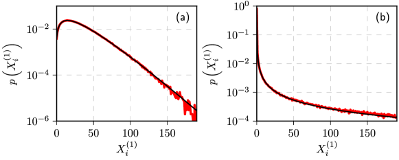
Figure 1: (color online) Comparison between the numerical PMFs of $X_{i}^{\left(1\right)}$ (red curves) against the Beta-binomial PMFs (black curves). Model parameter values: $N=3000$, $T=1$, $M=100$ and $C=N$ (in all cases), $\varepsilon^{\left(1\right)}=2$ (a) and $0.03$ (b). Assumed parameter values of the Beta-binomial distribution: $N=3000$, $\alpha=\varepsilon^{\left(1\right)}$ and $\beta=\left(M-1\right)\varepsilon^{\left(1\right)}$ (in all cases).

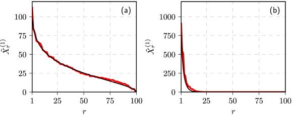
Figure 2: (color online) Comparison between the numerical CRSDs of $X_{i}^{\left(1\right)}$ (red curves) against the Beta-binomial RSDs (black curves). Numerical CRSDs were obtained from the same simulations as in Fig. 1. Assumed parameter values of the Beta-binomial distribution are also the same as in Fig. 1.

If $\frac{N}{M}<C<N$, we can no longer ignore the fact the number of agents within compartment, $N_{i}$, is capped. Consequently we can no longer simplify the sums in the total entry and exit rates, Eqs. (2) and (3), to a tractable form even for the simplest cases. Though it is possible to obtain stationary PMF for the specific cases by treating the model as one dimensional Markov chain or from detailed balance condition. Using the Markov chain approach we were able to find that for $T=1$ and $M=2$ PMF of $X_{i}^{\left(k\right)}$ precisely follows truncated Beta-binomial distribution (see Fig. 3). One can easily confirm this from detailed balance condition Eq. (4), which would now apply to a narrower interval $X_{i}^{\left(k\right)}\in\left[C,N^{\left(k\right)}-C-1\right]$. As the condition itself has not changed, in order to get stationary PMF in this case we just have to appropriately truncate the Beta-binomial PMF. Yet for other, more complicated cases, we were unable to discover a general pattern with either of the discussed approaches. Furthermore size of the Markov chain (the number of states) seems to grow exponentially with both $T$ and $M$. The number of recursive equations to be satisfied also seems to grow exponentially fast. Hence for realistic $N$, $T$ and $M$ it is not feasible to obtain an analytical result.

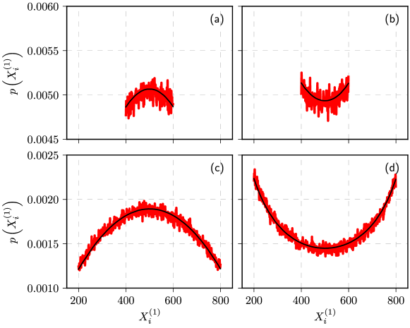
Figure 3: (color online) Comparison between the numerical PMFs of $X_{i}^{\left(1\right)}$ (red curves) against the truncated Beta-binomial PMFs (black curves). Model parameter values: $N=1000$, $T=1$ and $M=2$ (in all cases), $C=600$ ((a) and (b)) and $800$ ((c) and (d)), $\varepsilon^{\left(1\right)}=2$ ((a) and (c)) and $0.03$ ((b) and (d)). Assumed parameter values of the truncated Beta-binomial distribution: $N=1000$, $\alpha=\varepsilon$ and $\beta=\left(M-1\right)\varepsilon$, while allowing for $X_{i}^{\left(1\right)}\in\left[N-C,C\right]$ (in all cases).

In this model we have assumed that compartments are identical, while in the real world the compartments will not be identical. In the real world there will be a natural variation in number of people in spatial units, due to historical or geographical reasons. Also number of people in empirical data sets might be larger than numerical simulations could deal with (at least in reasonable computation time). For these reasons instead of making direct comparisons with the raw $X_{i}^{\left(k\right)}$, we introduce use a scaled variable, which we refer to as a population fraction:

$$f_{i}^{\left(k\right)}=\frac{X_{i}^{\left(k\right)}}{N_{i}}.$$ (7)

In the empirical context closest match to the population fraction would be the vote share, which in empirical works is defined as fraction of votes case for specific party or candidate during the given election. Obtaining closed form expression for the stationary distribution of $f_{i}^{\left(k\right)}$ is quite problematic, because even in the simplest case $f_{i}^{\left(k\right)}$ is a ratio of a Beta distributed random variable and a sum of correlated Beta distributed random variables. In mathematical statistics some results are known only for a very simple combinations of independent Beta random variables [54, 55]. Nevertheless at least for a few selected cases we see that $f_{i}^{\left(k\right)}$ has a stationary distribution which is well approximated by the Beta distribution (see Fig. 4), although the distribution parameter values must be fitted on case–by–case basis and some discrepancies are noticeable. Though notably the fitted parameter values for $f_{i}^{\left(k\right)}$, we have used Maximum Likelihood Estimation to obtain them, appear to be reasonably close to $\alpha=\varepsilon^{\left(k\right)}$ and $\beta=\left(\sum_{t=1}^{T}\varepsilon^{\left(t\right)}\right)-\varepsilon^{\left(k\right)}$.

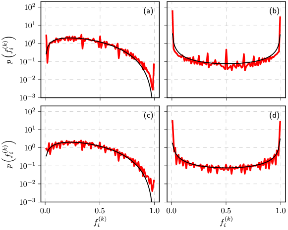
Figure 4: (color online) Fitting the numerical PDFs of $f_{i}^{\left(k\right)}$ (red curves) using PDF of Beta distribution (black curves). Model parameter values: $N^{\left(1\right)}=N^{\left(2\right)}=N^{\left(3\right)}=1000$ (there were $N=3000$ agents in total), $M=100$, $T=3$ and $\varepsilon^{\left(1\right)}=\varepsilon^{\left(2\right)}=\varepsilon^{\left(3\right)}=\varepsilon$ (in all cases), $C=N$ ((a) and (b)) and $C=35$ ((c) and (d)), $\varepsilon=2$ ((a) and (c)) and $0.03$ ((b) and (d)). Best fit parameter values for the Beta distribution: (a) $\alpha=1.69$ and $\beta=3.46$, (b) $\alpha=0.031$ and $\beta=0.055$, (c) $\alpha=1.76$ and $\beta=3.53$, (d) $\alpha=0.033$ and $\beta=0.055$.

3 Comparison with selected empirical data sets

In this section we use the compartmental model to fit the empirical census and electoral data. We take three subsets of UK census 2011 data (which can be obtained from the NOMIS website) and one subset of Lithuanian parliamentary election 1992 data (which can be obtained from a dedicated GitHub repository). These subsets were selected semi–randomly, namely we have ensured that all considered “groups” of people would be quite well represented and reasonably segregated. We have rejected some other randomly selected subsets, because they were either dominated by a single “group” or were too uniformly spread out.

The first example we consider is the ethnic group distribution over the postal districts (in total $155$ of them) in London (see Fig. 5). We consider three most well represented ethnic groups (White, Asian and Black), while combining less represented groups in to the other group. Members of mixed ethnic groups were assigned to either Asian, Black or the other group. In the simulation we have used $77345$ agents to represent $4856091$ people in the data set (approximately $1:60$ ratio). Other model parameter values are listed in the caption of Fig. 5.

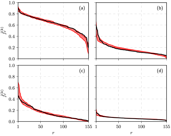
Figure 5: (color online) Comparison between the numerical CRSDs of $f_{i}^{\left(k\right)}$ (red shaded areas) against empirical CRSDs for the ethnic group distributions in London (black curves). Different sub–figures show the curves for the different considered ethnic groups: (a) White (index $w$), (b) Asian (index $a$), (c) Black (index $b)$ and (d) other (index $o$). Numerical results are reported using $95\%$ confidence interval, which spans the red shaded area. Model parameter values: $N^{\left(w\right)}=48515$, $N^{\left(a\right)}=12865$, $N^{\left(b\right)}=11470$ and $N^{\left(o\right)}=4495$ (there were $N=77345$ agents in total), $\varepsilon^{\left(w\right)}=2.5$, $\varepsilon^{\left(a\right)}=4$, $\varepsilon^{\left(b\right)}=1.5$, $\varepsilon^{\left(o\right)}=15$, $M=155$, $C=600$.

The second example we consider is the religious group distribution over the postal sectors ($109$ of them) in Leicester (see Fig. 6). We consider three groups: Christian, no religion and other religion. These groups were selected, because they were the most well represented. No religion other than Christianity was sufficiently well represented so all their followers were combined into the other religion group. In the simulation we have used $54391$ agents to represent $925071$ people in the data set (approximately $1:17$ ratio). Other model parameter values are listed in the caption of Fig. 6.

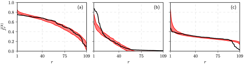
Figure 6: (color online) Comparison between the numerical CRSDs of $f_{i}^{\left(k\right)}$ (red shaded areas) against empirical CRSDs for the religious group distributions in Leicester (black curves). Different sub–figures show the curves for the different considered religious groups: (a) Christians (index $c$), (b) no religion (index $n$) and (c) other (index $o$). Numerical results are reported using $95\%$ confidence interval, which spans the red shaded area. Model parameter values: $N^{\left(c\right)}=30411$, $N^{\left(n\right)}=8829$ and $N^{\left(o\right)}=15151$ (there were $N=54391$ agents in total), $\varepsilon^{\left(c\right)}=2.5$, $\varepsilon^{\left(n\right)}=0.01$, $\varepsilon^{\left(o\right)}=50$, $M=109$, $C=600$.

The third and final UK census example is based on the National Statistics Socio–Economic Classification (abbr. NS–SEC). UK census 2011 data is available in the eight–class resolution, but we down scale to the three–class resolution to ensure that each class would be well represented. This gives us four groups: higher (class 1), intermediate (class 2), lower occupations (class 3) and long–term unemployed. We have ignored data regarding persons still in education and ones who have retired. In the simulation we have used $97000$ agents to represent $902970$ people in the data set (approximately $1:9$ ratio). In Fig. 7 we have plotted the employment class distribution over the postal sectors ($194$ of them) in Sheffield. Caption of the figure lists other parameter values used in the simulation.

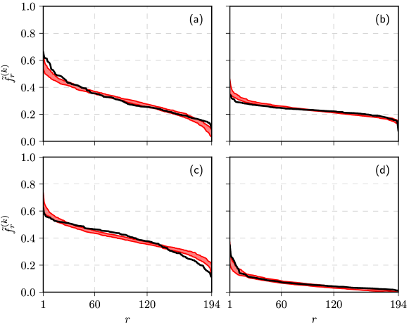
Figure 7: (color online) Comparison between the numerical CRSDs of $f_{i}^{\left(k\right)}$ (red shaded areas) against empirical CRSDs for the NS–SEC class distributions in Sheffield (black curves). Different sub–figures show the curves for the different considered NS–SEC classes: (a) higher occupations (index $1$), (b) intermediate occupations (index $2$), (c) lower occupations (index $3$) and (d) unemployed (index $u$). Numerical results are reported using $95\%$ confidence interval, which spans the red shaded area. Model parameter values: $N^{\left(1\right)}=29876$, $N^{\left(2\right)}=22310$, $N^{\left(3\right)}=38218$ and $N^{\left(u\right)}=6596$ (there were $N=97000$ agents in total), $\varepsilon^{\left(1\right)}=3$, $\varepsilon^{\left(2\right)}=50$, $\varepsilon^{\left(3\right)}=12$, $\varepsilon^{\left(u\right)}=2$, $M=194$, $C=600$.

For the last example we take a subset of Lithuanian parliamentary election 1992 data: the vote share distribution over the polling stations ($89$ of them) in Vilnius (see Fig. 8). As was done earlier in [38] we have selected three most successful parties to have their own groups, while all other less successful parties were combined into a single group. In the simulation we have used $44500$ agents to represent $177505$ voters in the data set (approximately $1:4$ ratio). Other model parameter values are listed in the caption of Fig. 8.

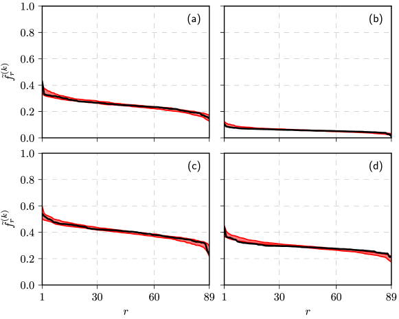
Figure 8: (color online) Comparison between the numerical CRSDs of $f_{i}^{\left(k\right)}$ (red shaded areas) against empirical vote share CRSDs observed in Vilnius during Lithuanian parliamentary election of 1992 (black curves). Different sub–figures show the curves for the different considered parties: (a) Sąjūdžio koalicija (index $s$), (b) Lietuvos krikščionių demokartų partija (index $l$), (c) Lietuvos demokratinė darbo partija (index $d$) and (d) other parties (index $o$). Numerical results are reported using $95\%$ confidence interval, which spans the red shaded area. Model parameter values: $N^{\left(s\right)}=11125$, $N^{\left(l\right)}=2581$, $N^{\left(d\right)}=17978$ and $N^{\left(o\right)}=12816$ (there were $N=44500$ agents in total), $\varepsilon^{\left(s\right)}=\varepsilon^{\left(l\right)}=\varepsilon^{\left(d\right)}=25$, $\varepsilon^{\left(o\right)}=75$, $M=89$, $C=600$.

As can be seen in the figures the compartmental model despite its simplicity is able to provide a rather good fits for the empirical data. Some deviations are observed due to variety of factors. Namely, we have neglected in–type heterogeneity, while not all people of the same “group” would have the same tendency to migrate independently. Also not all “classifications” of the people are equally important for the migration purposes (e.g., sex would be not important at all) or multiple “classifications” might play a role at the same time (e.g., if the person strongly identifies with both his ethnicity and religious beliefs).

4 Conclusions

In the [33] Fernandez-Garcia and coauthors have asked whether the voter model is a model for voters. Here we have proposed a simple compartmental model based on the noisy voter model with the aim to provide our answer to this question. We have assumed that agents (voters) have fixed types (cultural traits or opinions), but are able to migrate between the compartments (residential areas or electoral districts). In such model there is no actual opinion dynamics only spatial organization (migration). While exploring the general statistical properties of the proposed model we have shown that in some cases the model generates Beta distributed random variables, which is consistent with the empirical observations. To strengthen our argument we have used the compartmental model to provide a rather good fits for the empirical census and electoral data. We believe that this allows us to conclude that the spatial variations in the electoral data can arise purely from the spatial organization patterns. So, while the voter model is assumed to be a model for voters similar patterns can be recovered even without any actual opinion dynamics. Alternatively, the actual opinion exchange process could be described by a different model, maybe even a convergent model.

The proposed model is quite simple and invites variety of further explorations both from numerical and analytical perspectives. From numerical perspective it would reasonable to give the compartments some actual spatial structure and explore the arising spatial correlations. This would also allow to make comparisons to the human mobility models. While from analytical perspective it would be quite useful to establish a technique to derive the compartmental rank–size distributions, which emerge after an almost infinite time. From both perspectives an important future consideration would be to allow the agents to change their “types” and see what dynamics arise from the two competing processes (compartmental organization and opinion exchange).

References

- [1] S. Galam, “Sociophysics: A review of Galam models,” International Journal of Modern Physics C, vol. 19, no. 03, p. 409, 2008.
- [2] C. Castellano, S. Fortunato, and V. Loreto, “Statistical physics of social dynamics,” Reviews of Modern Physics, vol. 81, pp. 591–646, 2009.
- [3] D. Stauffer, “A biased review of sociophysics,” Journal of Statistical Physics, 2013.
- [4] A. Flache, M. Mas, T. Feliciani, E. Chattoe-Brown, G. Deffuant, S. Huet, and J. Lorenz, “Models of social influence: Towards the next frontiers,” The Journal of Artificial Society and Social Simulation, vol. 20, no. 4, p. 2, 2017.
- [5] A. Sirbu, V. Loreto, V. D. P. Servedio, and F. Tria, Opinion dynamics: models, extensions and external effects, ch. 17, pp. 363–401. Springer International Publishing, 2017.
- [6] A. Baronchelli, “The emergence of consensus: a primer,” Royal Society Open Science, vol. 5, p. 172189, 2018.
- [7] A. Jedrzejewski and K. Sznajd-Weron, “Statistical physics of opinion formation: Is it a SPOOF?,” Comptes Rendus Physique, 2019.
- [8] S. Galam and F. Jacobs, “The role of inflexible minorities in the breaking of democratic opinion dynamics,” Physica A, vol. 381, pp. 366 – 376, 2007.
- [9] M. Mobilia, A. Petersen, and S. Redner, “On the role of zealotry in the voter model,” Journal of Statistical Mechanics: Theory and Experiment, vol. 2007, no. 08, p. P08029, 2007.
- [10] A. P. Kirman, “Ants, rationality and recruitment,” Quarterly Journal of Economics, vol. 108, pp. 137–156, 1993.
- [11] L. B. Granovsky and N. Madras, “The noisy voter model,” Stochastic Processes and their Applications, vol. 55, no. 1, pp. 23–43, 1995.
- [12] P. R. Nail and K. Sznajd-Weron, “The diamond model of social response within an agent-based approach,” Acta Physica Polonica A, vol. 129, no. 5, pp. 1050–1054, 2016.
- [13] P. Duggins, “A psychologically-motivated model of opinion change with applications to American politics,” Journal of Artificial Societies and Social Simulation, vol. 20, no. 1, p. 13, 2017.
- [14] A. Kononovicius and V. Gontis, “Agent based reasoning for the non-linear stochastic models of long-range memory,” Physica A, vol. 391, no. 4, pp. 1309–1314, 2012.
- [15] A. Kononovicius and J. Ruseckas, “Continuous transition from the extensive to the non-extensive statistics in an agent-based herding model,” European Physics Journal B, vol. 87, no. 8, p. 169, 2014.
- [16] A. Kononovicius and V. Gontis, “Control of the socio-economic systems using herding interactions,” Physica A, vol. 405, pp. 80–84, 2014.
- [17] D. Harmon, M. Lagi, M. A. M. de Aguiar, D. D. Chinellato, D. Braha, I. R. Epstein, and Y. Bar-Yam, “Anticipating economic market crises using measures of collective panic,” PLOS ONE, vol. 10, no. 7, pp. 1–27, 2015.
- [18] A. Carro, R. Toral, and M. San Miguel, “The noisy voter model on complex networks,” Scientific Reports, vol. 6, p. 24775, 2016.
- [19] S. Galam, “The invisible hand and the rational agent are behind bubbles and crashes,” Chaos, Solitons and Fractals, vol. 88, pp. 209–217, 2016.
- [20] N. Khalil, M. San Miguel, and R. Toral, “Zealots in the mean-field noisy voter model,” Physical Review E, vol. 97, p. 012310, 2018.
- [21] A. F. Peralta, A. Carro, M. San Miguel, and R. Toral, “Analytical and numerical study of the non-linear noisy voter model on complex networks,” Chaos, vol. 28, p. 075516, 2018.
- [22] A. L. M. Vilela, C. Wang, K. P. Nelson, and H. E. Stanley, “Majority-vote model for financial markets,” Physica A, 2018.
- [23] A. L. M. Vilela and H. E. Stanley, “Effect of strong opinions on the dynamics of the majority-vote model,” Scientific Reports, vol. 8, p. 8709, 2018.
- [24] O. Artime, A. Carro, A. F. Peralta, J. J. Ramasco, M. San Miguel, and R. Toral, “Herding and idiosyncratic choices: nonlinearity and aging-induced transitions in the noisy voter model.” Available as arXiv:1812.05378 [physics.soc-ph], 2019.
- [25] A. L. M. Vilela, C. Wang, K. P. Nelson, and H. E. Stanley, “Majority-vote model for financial markets,” Physics A, vol. 515, pp. 762–770, 2019.
- [26] T. Schelling, Some fun, thirty-five years ago, vol. 2, pp. 1639 – 1644. Elsevier, 2006.
- [27] M. Ausloos and F. Petroni, “Statistical dynamics of religions and adherents,” EPL, vol. 77, no. 3, p. 38002, 2007.
- [28] E. Hatna and I. Benenson, “The Schelling model of ethnic residential dynamics: Beyond the integrated - segregated dichotomy of patterns,” Journal of Artificial Societies and Social Simulation, vol. 15, no. 1, p. 6, 2012.
- [29] M. Ausloos, C. Herteliu, and B. Ileanu, “Breakdown of Benford’s law for birth data,” Physica A, vol. 419, pp. 736–745, 2015.
- [30] E. Barter and T. Gross, “Manifold cities: Social variables of urban areas in the UK,” Proceedings of the Royal Society A, vol. 475, no. 2221, p. 20180615, 2019.
- [31] C. Borghesi and J. Bouchaud, “Spatial correlations in vote statistics: a diffusive field model for decision-making,” European Physical Journal B, vol. 75, no. 3, pp. 395–404, 2010.
- [32] C. Borghesi, J.-C. Raynal, and J. P. Bouchaud, “Election turnout statistics in many countries: similarities, differences, and a diffusive field model for decision-making,” PLoS ONE, vol. 7, p. e36289, 2012.
- [33] J. Fernandez-Gracia, K. Suchecki, J. J. Ramasco, M. San Miguel, and V. M. Eguiluz, “Is the voter model a model for voters?,” Physical Review Letters, vol. 112, p. 158701, 2014.
- [34] F. Sano, M. Hisakado, and S. Mori, “Mean field voter model of election to the house of representatives in Japan,” in JPS Conference Proceedings, vol. 16, p. 011016, The Physical Society of Japan, 2017.
- [35] D. Braha and M. A. M. de Aguiar, “Voting contagion: Modeling and analysis of a century of u.s. presidential elections,” PLOS ONE, vol. 12, no. 5, pp. 1–30, 2017.
- [36] T. Fenner, M. Levene, and G. Loizou, “A multiplicative process for generating the rank-order distribution of UK election results,” Quality and Quantity, pp. 1–11, 2017.
- [37] T. Fenner, E. Kaufmann, M. Levene, and G. Loizou, “A multiplicative process for generating a beta-like survival function with application to the UK 2016 EU referendum results,” International Journal of Modern Physics C, vol. 28, p. 1750132, 2017.
- [38] A. Kononovicius, “Empirical analysis and agent-based modeling of Lithuanian parliamentary elections,” Complexity, vol. 2017, p. 7354642, 2017.
- [39] J. Michaud and A. Szilva, “Social influence with recurrent mobility and multiple options,” Physcal Review E, vol. 97, p. 062313, 2018.
- [40] S. Mori, M. Hisakado, and K. Nakayama, “Voter model on networks and the multivariate beta distribution,” Physical Review E, vol. 99, p. 052307, 2019.
- [41] B. E. Hansen, “Recounts from undervotes: Evidence from the 2000 presidential election,” Journal of the American Statistical Association, vol. 98, no. 462, pp. 292–298, 2003.
- [42] S. E. Rigdon, S. H. Jacobson, E. C. Tam Cho, W. K. abd Sewell, and C. J. Rigdon, “A Bayesian prediction model for the U.S. presidential election,” American Politics Research, vol. 37, no. 4, pp. 700–724, 2009.
- [43] A. Kononovicius, “Modeling of the parties’ vote share distributions,” Acta Physica Polonica A, vol. 133, no. 6, pp. 1450–1458, 2018.
- [44] M. Downes, L. C. Gurrin, D. R. English, J. Pirkis, D. Currier, M. J. Spittal, and J. B. Carlin, “Multilevel regression and poststratification: A modeling approach to estimating population quantities from highly selected survey samples,” American Journal of Epidemiology, vol. 187, no. 8, pp. 1780–1790, 2018.
- [45] H. Barbosa, M. Barthelemy, G. Ghoshal, C. R. James, M. Lenormand, T. Louail, R. Menezes, J. J. Ramasco, F. Simini, and M. Tomasini, “Human mobility: Models and applications,” Physics Reports, vol. 734, pp. 1 – 74, 2018.
- [46] G. K. Zipf, “The P<sub>1</sub> P<sub>2</sub>/D hypothesis: On the intercity movement of persons,” American Sociological Review, vol. 11, no. 6, pp. 677–686, 1946.
- [47] W.-S. Jung, F. Wang, and H. E. Stanley, “Gravity model in the korean highway,” EPL, vol. 81, no. 4, p. 48005, 2008.
- [48] D. Braha, B. Stacey, and Y. Bar-Yam, “Corporate competition: A self-organized network,” Social Networks, vol. 33, no. 3, pp. 219 – 230, 2011.
- [49] F. Simini, M. C. Gonzalez, A. Maritan, and A. L. Barabasi, “A universal model for mobility and migration patterns,” Nature, vol. 484, pp. 96–100, 2012.
- [50] L. Pappalardo, S. Rinzivillo, and F. Simini, “Human mobility modelling: Exploration and preferential return meet the gravity model,” Procedia Computer Science, vol. 83, pp. 934–939, 2016.
- [51] N. Metropolis, A. W. Rosnbluth, M. N. Rosenbluth, and A. H. Teller, “Equation of state calculations by fast computing machines,” Journal of Chemical Physics, vol. 21, p. 1087, 1953.
- [52] K. Kawasaki, “Diffusion constants near the critical point for time-dependent Ising models. I,” Physical Review, vol. 145, pp. 224–230, 1966.
- [53] K. Kawasaki, “Diffusion constants near the critical point for time-dependent Ising models. II,” Physical Review, vol. 148, pp. 375–381, 1966.
- [54] T. G. Pham and N. Turkkan, “Reliability of a standby system with beta-distributed component lives,” IEEE Transactions on Reliability, vol. 43, no. 1, pp. 71–75, 1994.
- [55] T. Pham-Gia, “Distributions of the ratios of independent beta variables and applications,” Communications in Statistics - Theory and Methods, vol. 29, no. 12, pp. 2693–2715, 2000.