Improving Textual Network Embedding with Global Attention
via Optimal Transport

Abstract

Constituting highly informative network embeddings is an important tool for network analysis. It encodes network topology, along with other useful side information, into low-dimensional node-based feature representations that can be exploited by statistical modeling. This work focuses on learning context-aware network embeddings augmented with text data. We reformulate the network-embedding problem, and present two novel strategies to improve over traditional attention mechanisms: ($i$) a content-aware sparse attention module based on optimal transport, and ($ii$) a high-level attention parsing module. Our approach yields naturally sparse and self-normalized relational inference. It can capture long-term interactions between sequences, thus addressing the challenges faced by existing textual network embedding schemes. Extensive experiments are conducted to demonstrate our model can consistently outperform alternative state-of-the-art methods.

1 Introduction

When performing network embedding, one maps network nodes into vector representations that reside in a low-dimensional latent space. Such techniques seek to encode topological information of the network into the embedding, such as affinity (Tang and Liu, 2009), local interactions (e.g, local neighborhoods) (Perozzi et al., 2014), and high-level properties such as community structure (Wang et al., 2017). Relative to classical network-representation learning schemes (Zhang et al., 2018a), network embeddings provide a more fine-grained representation that can be easily repurposed for other downstream applications (e.g., node classification, link prediction, content recommendation and anomaly detection).

For real-world networks, one naturally may have access to rich side information about each node. Of particular interest are textual networks, where the side information comes in the form of natural language sequences (Le and Lauw, 2014). For example, user profiles or their online posts on social networks (e.g., Facebook, Twitter), and documents in citation networks (e.g., Cora, arXiv). The integration of text information promises to significantly improve embeddings derived solely from the noisy, sparse edge representations (Yang et al., 2015).

Recent work has started to explore the joint embedding of network nodes and the associated text for abstracting more informative representations. Yang et al. (2015) reformulated DeepWalk embedding as a matrix factorization problem, and fused text-embedding into the solution, while Sun et al. (2016) augmented the network with documents as auxiliary nodes. Apart from direct embedding of the text content, one can first model the topics of the associated text (Blei et al., 2003) and then supply the predicted labels to facilitate embedding (Tu et al., 2016).

Many important downstream applications of network embeddings are context-dependent, since a static vector representation of the nodes adapts to the changing context less effectively (Tu et al., 2017). For example, the interactions between social network users are context-dependent (e.g., family, work, interests), and contextualized user profiling can promote the specificity of recommendation systems. This motivates context-aware embedding techniques, such as CANE (Tu et al., 2017), where the vector embedding dynamically depends on the context. For textual networks, the associated texts are natural candidates for context. CANE introduced a simple mutual attention weighting mechanism to derive context-aware dynamic embeddings for link prediction. Following the CANE setup, WANE (Shen et al., 2018) further improved the contextualized embedding, by considering fine-grained text alignment.

Despite the promising results reported thus far, we identify three major limitations of existing context-aware network embedding solutions. First, mutual (or cross) attentions are computed from pairwise similarities between local text embeddings (word/phrase matching), whereas global sequence-level modeling is known to be more favorable across a wide range of NLP tasks  (MacCartney and Manning, 2009; Liu et al., 2018; Malakasiotis and Androutsopoulos, 2007; Guo et al., 2018). Second, related to the above point, low-level affinity scores are directly used as mutual attention without considering any high-level parsing. Such an over-simplified operation denies desirable features, such as noise suppression and relational inference (Santoro et al., 2017), thereby compromising model performance. Third, mutual attention based on common similarity measures (e.g., cosine similarity) typically yields dense attention matrices, while psychological and computational evidence suggests a sparse attention mechanism functions more effectively (Martins and Astudillo, 2016; Niculae and Blondel, 2017). Thus such naive similarity-based approaches can be suboptimal, since they are more likely to incorporate irrelevant word/phrase matching.

This work represents an attempt to improve context-aware textual network embedding, by addressing the above issues. Our contributions include: ($i$) We present a principled and more-general formulation of the network embedding problem, under reproducing kernel Hilbert spaces (RKHS) learning; this formulation clarifies aspects of the existing literature and provides a flexible framework for future extensions. ($ii$) A novel global sequence-level matching scheme is proposed, based on optimal transport, which matches key concepts between text sequences in a sparse attentive manner. ($iii$) We develop a high-level attention-parsing mechanism that operates on top of low-level attention, which is capable of capturing long-term interactions and allows relational inference for better contextualization. We term our model Global Attention Network Embedding (GANE). To validate the effectiveness of GANE, we benchmarked our models against state-of-the-art counterparts on multiple datasets. Our models consistently outperform competing methods.

2 Problem setup

We introduce basic notation and definitions used in this work.

Textual networks.

Let $\mathcal{G}=(\mathcal{V},\mathcal{E},\mathcal{T})$ be our textual network, where $\mathcal{V}$ is the set of nodes, $\mathcal{E}\subseteq\mathcal{V}\times\mathcal{V}$ are the edges between the nodes, and $\mathcal{T}=\{S_{v}\}_{v\in\mathcal{V}}$ are the text data associated with each node. We use $S_{v}=[\omega_{1},\cdots,\omega_{n_{v}}]$ to denote the token sequence associated with node $v\in\mathcal{V}$, of length $n_{v}=|S_{v}|$ where $|\cdot|$ denotes the counting measure. To simplify subsequent discussion, we assume all tokens have been pre-embedded in a $p$-dimensional feature space. As such, $S_{v}$ can be directly regarded as a $\mathbb{R}^{p\times n_{v}}$ matrix tensor. We use $\{u,v\}$ to index the nodes throughout the paper. We consider directed unsigned graphs, meaning that for each edge pair $(u,v)\in\mathcal{E}$ there is a nonnegative weight $w_{uv}$ associated with it, and $w_{uv}$ does not necessarily equal $w_{vu}$.

Textual network embedding.

The goal of textual network embedding is to identify a $d$-dimensional embedding vector ${\bm{z}}_{v}\in\mathbb{R}^{d}$ for each node $v\in\mathcal{V}$, which encodes network topology ($\mathcal{E}$) via leveraging information from the associated text ($\mathcal{T}$). In mathematical terms, we want to learn an encoding (embedding) scheme ${\bf Z}_{\mathcal{G}}\triangleq\{{\bm{z}}_{v}=\text{Enc}(v;\mathcal{G})\}_{v\in\mathcal{V}}$ and a probabilistic decoding model with likelihood $p_{\theta}(E;{\bf Z})$, where $E\subseteq\mathcal{V}\times\mathcal{V}$ is a random network topology for node set $\mathcal{V}$, such that the likelihood for the observed topology $p_{\theta}(\mathcal{E}|{\bf Z}_{\mathcal{G}})$ is high. Note that for efficient coding schemes, the embedding dimension is much smaller than the network size (i.e., $d\ll|\mathcal{V}|$). In a more general setup, the decoding objective can be replaced with $p_{\theta}(\mathcal{A}|{\bf Z})$, where $\mathcal{A}$ denotes observed attributes of interest (e.g., node label, community structure, etc.).

Context-aware embedding.

One way to promote coding efficiency is to contextualize the embeddings. More specifically, the embeddings additionally depend on an exogenous context $c$. To distinguish it from the context-free embedding ${\bm{z}}_{u}$, we denote the context-aware embedding as ${\bm{z}}_{u|c}$, where $c$ is the context. For textual networks, when the embedding objective is network topology reconstruction, a natural choice is to treat the text as context (Tu et al., 2017). In particular, when modeling the edge $w_{uv}$, $S_{v}$ and $S_{u}$ are respectively treated as the context for context-aware embeddings ${\bm{z}}_{u|c}$ and ${\bm{z}}_{v|c}$, which are then used in the prediction of edge likelihood.

Attention & text alignment.

Much content can be contained in a single text sequence, and retrieving them with a fixed length feature vector can be challenging. A more flexible solution is to employ an attention mechanism, which only attends to content that is relevant to a specific query  Vaswani et al. (2017). Specifically, attention models leverage a gating mechanism to de-emphasize irrelevant parts in the input; this method pools information only from the useful text, which is also a fixed length vector but that only encodes information with respect to one specific content  Santos et al. (2016). Popular choices of attention include normalized similarities in the feature space (e.g., Softmax normalized cosine distances). For two text sequences, one can build a mutual attention by cross-relating the content from the respective text  (Santoro et al., 2017). In text alignment, one further represents the content from one text sequence using the mutual attention based attentive-pooling on the other sequence (Shen et al., 2018).

Optimal transport (OT).

Consider ${\bm{\mu}}=\{({\bm{x}}_{i},\mu_{i})\}_{i=1}^{n}$ and ${\bm{\nu}}=\{({\bm{y}}_{j},\nu_{j})\}_{j=1}^{m}$, a set of locations and their associated nonnegative mass (we assume $\sum_{i}\mu_{i}=\sum_{j}\nu_{j}=1$). We call $\pi\in\mathbb{R}_{+}^{n\times m}$ a valid transport plan if it properly redistributes mass from ${\bm{\mu}}$ to ${\bm{\nu}}$, i.e., $\sum_{i}\pi_{ij}=\nu_{j}$ and $\sum_{j}\pi_{ij}=\mu_{i}$. In other words, $\pi$ breaks mass at $\{{\bm{x}}_{i}\}$ into smaller parts and transports $\pi_{ij}$ units of ${\bm{x}}_{i}$ to ${\bm{y}}_{j}$. Given a cost function $c({\bm{x}},{\bm{y}})$ for transporting unit mass from ${\bm{x}}$ to ${\bm{y}}$, discretized OT solves the following constrained optimization for an optimal transport plan $\pi^{*}$ (Peyré et al., 2017):

$$\mathcal{D}_{c}({\bm{\mu}},{\bm{\nu}})=\inf_{\pi\in\Pi(\mu,\nu)}\left\{\sum_{ij}\pi_{ij}c({\bm{x}}_{i},{\bm{y}}_{j})\right\}\,,$$ (1)

where $\Pi({\bm{\mu}},{\bm{\nu}})$ denotes the set of all viable transport plans. Note that $c({\bm{x}},{\bm{y}})$ is a distance metric on $\mathcal{X}$, and $D_{c}({\bm{\mu}},{\bm{\nu}})$ induces a distance metric on the space of probability distributions supported on $\mathcal{X}$, commonly known as the Wasserstein distance (Villani, 2008). Popular choices of cost include Euclidean cost $\|{\bm{x}}-{\bm{y}}\|_{2}^{2}$ for general probabilistic learning (Gulrajani et al., 2017) and cosine similarity cost $\cos({\bm{x}},{\bm{y}})$ for natural language models (Chen et al., 2018). Computationally, OT plans are often approximated with Sinkhorn-type iterative schemes (Cuturi, 2013). Algorithm 1 summarizes a particular variant used in our study (Xie et al., 2018).

Algorithm 1 Optimal transport solver (SolveOT)

1:Input: Sentence matrices ${\bf S}=\{{\bm{w}}_{i}\}_{1}^{n}$, ${\bf S}^{\prime}=\{{\bm{w}}^{\prime}_{j}\}_{1}^{m}$      and generalized stepsize $1/\beta$,

2:$\bm{\sigma}=\frac{1}{m}\mathbf{1_{m}}$, ${\bf T}^{(1)}=\mathbf{1_{n}}\mathbf{1_{m}}^{\top}$

3:${\bf C}_{ij}=c({\bm{z}}_{i},{\bm{z}}^{\prime}_{j})$, ${\bf A}_{ij}={\rm e}^{-\frac{{\bf C}_{ij}}{\beta}}$

4:for $t=1,2,3\ldots$ do

5:     ${\bf Q}={\bf A}\odot{\bf T}^{(t)}$ // $\odot$ is Hadamard product

6:     for $k=1,\ldots K$ do // $K=1$ in practice

7:         $\bm{\delta}=\frac{1}{n{\bf Q}{\bm{\sigma}}}$, $\bm{\sigma}=\frac{1}{m{\bf Q}^{\top}\bm{\delta}}$

8:     end for

9:     ${\bf T}^{(t+1)}=\text{diag}(\bm{\delta}){\bf Q}\text{diag}(\bm{\sigma})$

10:end for

11:Return ${\bf T}$

3 Proposed Method

3.1 Model framework overview

To capture both the topological information (network structure $\mathcal{E}$) and the semantic information (text content $\mathcal{T}$) in the textual network embedding, we explicitly model two types of embeddings for each node $v\in\mathcal{V}$: ($i$) the topological embedding ${\bm{z}}_{u}^{t}$, and ($ii$) the semantic embedding ${\bm{z}}_{u}^{s}$. The final embedding is constructed by concatenating the topological and semantic embeddings, i.e., ${\bm{z}}_{u}=[{\bm{z}}_{u}^{t};{\bm{z}}_{u}^{s}]$. We consider the topological embedding ${\bm{z}}^{t}$ as a static property of the node, fixed regardless of the context. On the other hand, the semantic embedding ${\bm{z}}^{s}$ dynamically depends on the context, which is the focus of this study.

Motivated by the work of (Tu et al., 2017), we consider the following probabilistic objective to train the network embeddings:

$$\ell(\Theta)=\mathbb{E}_{e\sim\mathcal{E}}\left\{\ell(e;\Theta)\right\},\vspace{-2mm}$$ (2)

where $e=(u,v)$ represents sampled edges from the network and $\Theta=\{{\bf Z},\theta\}$ is the collection of model parameters. The edge loss $\ell(e;\Theta)$ is given by the cross entropy

$$\ell(e_{uv};\Theta)=-w_{uv}\log p_{\Theta}(u|v),$$ (3)

where $p_{\Theta}(u|v)$ denotes the conditional likelihood of observing a (weighted) link between nodes $u$ and $v$, with the latter serving as the context. More specifically,

$$p_{\Theta}(u|v)=\langle{\bm{z}}_{u},{\bm{z}}_{v}\rangle-\log(Z),\vspace{-2mm}$$ (4)

where $Z=\sum_{u^{\prime}\in\mathcal{V}}\exp(\langle{\bm{z}}_{u^{\prime}},{\bm{z}}_{v}\rangle)$ is the normalizing constant and $\langle\cdot,\cdot\rangle$ is an inner product operation, to be defined momentarily. Note here we have suppressed the dependency on $\Theta$ to simplify notation.

To capture both the topological and semantic information, along with their interactions, we propose to use the following decomposition for our inner product term:

$$\begin{array}[]{l}\langle{\bm{z}}_{u},{\bm{z}}_{v}\rangle=\underbrace{\langle{\bm{z}}_{u}^{t},{\bm{z}}_{v}^{t}\rangle_{tt}}_{\text{topology}}+\underbrace{\langle{\bm{z}}_{u}^{s},{\bm{z}}_{v}^{s}\rangle_{ss}}_{\text{semantic}}+\\ \hskip 50.00008pt\underbrace{\langle{\bm{z}}_{u}^{t},{\bm{z}}_{v}^{s}\rangle_{ts}+\langle{\bm{z}}_{u}^{s},{\bm{z}}_{v}^{t}\rangle_{st}}_{\text{interaction}}\end{array}\vspace{-2mm}$$ (5)

Here we use $\langle{\bm{z}}_{u}^{a},{\bm{z}}_{v}^{b}\rangle_{ab}\,,a,b\in\{s,t\}$ to denote the inner product evaluation between the two feature embeddings ${\bm{z}}_{u}^{a}$ and ${\bm{z}}_{v}^{b}$, which can be defined by a semi-positive-definite kernel function $\kappa_{ab}({\bm{z}}_{u}^{a},{\bm{z}}_{v}^{b})$  (Alvarez et al., 2012), e.g., Euclidean kernel, Gaussian RBF, IMQ kernel, etc. Note that for $a\neq b$, ${\bm{z}}_{u}^{a}$ and ${\bm{z}}_{v}^{b}$ do not reside on the same feature space. As such, embeddings are first mapped to the same feature space for inner product evaluation. In this study, we use the Euclidean kernel

$$\langle{\bm{x}}_{1},{\bm{x}}_{2}\rangle_{\mathcal{X}}={\bm{x}}_{1}^{T}{\bm{x}}_{2}\vspace{-2mm}$$

for inner product evaluation with ${\bm{x}}_{1},{\bm{x}}_{2}\in\mathcal{X}\subseteq\mathbb{R}^{d}$, and linear mapping

$$\langle{\bm{x}},{\bm{y}}\rangle_{\mathcal{X}\mathcal{Y}}=\langle{\bm{x}},{\bf A}{\bm{y}}\rangle_{\mathcal{X}},\text{ where }{\bf A}\in\mathbb{R}^{d\times d^{\prime}}\vspace{-2mm}$$

for feature space realignment with ${\bm{x}}\in\mathcal{X}\subseteq\mathbb{R}^{d},{\bm{y}}\in\mathcal{Y}\subseteq\mathbb{R}^{d^{\prime}}$. Here ${\bf A}$ is a trainable parameter, and throughout this paper we omit the bias terms in linear maps to avoid notational clutter.

Note that our solution differs from existing network-embedding models in that: ($i$) our objective is a principled likelihood loss, while prior works heuristically combine the losses of four different models  (Tu et al., 2017), which may fail to capture the non-trivial interactions between the fixed and dynamic embeddings; and ($ii$) we present a formal derivation of network embedding in a reproducing kernel Hilbert space.

Negative sampling.

Direct optimization of (3) requires summing over all nodes in the network, which can be computationally infeasible for large-scale networks. To alleviate this issue, we consider other more computationally efficient surrogate objectives. In particular, we adopt the negative sampling approach (Mikolov et al., 2013), which replaces the bottleneck Softmax with a more tractable approximation given by

$$\begin{array}[]{l}\log p(v|u)\approx\log\sigma(\langle{\bm{z}}_{u},{\bm{z}}_{v}\rangle)+\\[3.0pt] \hskip 50.00008pt\sum_{j=1}^{K}\mathbb{E}_{v_{k}\sim p_{n}}[\log\sigma(-\langle{\bm{z}}_{u},{\bm{z}}_{v_{k}}\rangle)],\end{array}\vspace{-2mm}$$ (6)

where $\sigma(x)=\frac{1}{1+\exp(-x)}$ is the sigmoid function, and $p_{n}(v)$ is a noise distribution over the nodes. Negative sampling can be considered as a special variant of noise contrastive estimation (Gutmann and Hyvärinen, 2010), which seeks to recover the ground-truth likelihood by contrasting data samples with noise samples, thereby bypassing the need to compute the normalizing constant. As the number of noise samples $K$ goes to infinity, this approximation becomes exact (Goldberg and Levy, 2014). Following the practice of Mikolov et al. (2013), we set our noise distribution to $p_{n}(v)\propto d_{v}^{\frac{3}{4}}$, where $d_{v}$ denotes the out-degree of node $v$.

Context matching.

We argue that a key to the context-aware network embedding is the design of an effective attention mechanism, which cross-matches the relevant content between the node’s associated text and the context. Over-simplified dot-product attention limits the potential of existing textual network embedding schemes. In the following sections, we present two novel, efficient attention designs that fulfill the desiderata listed in our Introduction. Our discussion follows the setup used in CANE (Tu et al., 2017) and WANE (Shen et al., 2018), where the text from the interacting node is used as the context. Generalization to other forms of context is straightforward.

3.2 Optimal-transport-based matching

Figure 1: Schematic of the proposed mutual attention mechanism. In this setup, bag-of-words feature matchings are explicitly abstracted to infer the relationship between vertices.

We first consider reformulating content matching as an optimal transport problem, and then re-purpose the transport plan as our attention score to aggregate context-dependent information. More specifically, we see a node’s text and context as two (discrete) distributions over the content space. Related content will be matched in the sense that they yield a higher weight in the optimal transport plan $\pi^{*}$. The following two properties make the optimal transport plan more appealing for use as attention score. ($i$) Sparsity: when solved exactly, $\pi^{*}$ is a sparse matrix with at most $(2m-1)$ non-zero elements, where $m$ is the number of contents (Brualdi et al. (1991), $\S 8.1.3$); ($ii$) Self-normalized: row-sum and column-sum equal the respective marginal distributions.

Implementation-wise, we first feed embedded text sequence $S_{u}$ and context sequence $S_{v}$ into our OT solver to compute the OT plan,

$${\bf T}_{uv}=\text{SolveOT}(S_{u},S_{v})\in\mathbb{R}^{n_{u}\times n_{v}}.\vspace{-2mm}$$ (7)

Note that here we treat pre-embedded sequence $S_{u}$ as $n_{u}$ point masses in the feature space, each with weight $1/n_{u}$, and similarly for $S_{v}$. Next we “transport” the semantic content from context $S_{v}$ according to the estimated OT plan with matrix multiplication

$$S_{u\leftarrow v}={\bf T}_{uv}S_{v}\in\mathbb{R}^{n_{u}\times p}\,,\vspace{-2mm}$$ (8)

where we have treated $S_{v}$ as a $\mathbb{R}^{n_{v}\times p}$ matrix. Intuitively, this operation aligns the context with the target text sequence via averaging the context semantic embeddings with respect to the OT plan for each content element in $S_{u}$. To finalize the contextualized embedding, we aggregate the information from both $S_{u}$ and the aligned $S_{u\leftarrow v}$ with an operator $F_{\text{agg}}$,

$${\bm{z}}_{u|v}=F_{\text{agg}}(S_{u},S_{u\leftarrow v})\in\mathbb{R}^{d\times 1}.\vspace{-2mm}$$ (9)

In this case, we practice the following simple aggregation strategy: first concatenate $S_{u}$ and the aligned $S_{u\leftarrow v}$ along the feature dimension, and then take max-pooling along the temporal dimension to reduce the feature vector into a $2p$ vector, followed by a linear mapping to project the embedding vector to the desired dimensionality.

3.3 Attention parsing

Direct application of attention scores based on a low-level similarity-based matching criteria (e.g., dot-product attention) can be problematic in a number of ways: ($i$) low-level attention scores can be noisy (i.e., spurious matchings), and ($ii$) similarity-matching does not allow relational inference. To better understand these points, consider the following cases. For ($i$), if the sequence embeddings used do not explicitly address the syntactic structure of the text, a relatively dense attention score matrix can be expected. For ($ii$), consider the case when the context is a query, and the matching appears as a cue in the node’s text data; then the information needed is actually in the vicinity rather than the exact matching location (e.g., shifted a few steps ahead). Inspired by the work of Wang et al. (2018), we propose a new mechanism called attention parsing to address the aforementioned issues.

As the name suggests, attention parsing re-calibrates the raw low-level attention scores to better integrate the information. To this end, we conceptually treat the raw attention matrix ${\bf T}_{\text{raw}}$ as a two-dimensional image and apply convolutional filters to it:

$${\bf H}=\text{ReLU}(\text{Conv2d}({\bf T}_{\text{raw}},{\bf W}_{F}))\in\mathbb{R}^{n_{u}\times n_{v}\times c}\,,\vspace{-1mm}$$ (10)

where ${\bf W}_{F}\in\mathbb{R}^{h\times w\times c}$ denotes the filter banks with $h,w$ and $c$ respectively as window sizes and channel number. We can stack more convolutional layers, break sequence embedding dimensions to allow multi-group (channel) low-level attention as input, or introduce more-sophisticated model architectures (e.g., ResNet (He et al., 2016), Transformer Vaswani et al. (2017), etc.) to enhance our model. For now, we focus on the simplest model described above, for the sake of demonstration.

With ${\bf H}\in\mathbb{R}^{n_{u}\times n_{v}\times c}$ as the high-level representation of attention, our next step is to reduce it to a weight vector to align information from the context $S_{v}$. We apply a max-pooling operation with respect to the context dimension, followed by a linear map to get the logits ${\bm{h}}\in\mathbb{R}^{n_{u}\times 1}$ of the weights

$${\bm{h}}=\text{MaxPool}({\bf H},\text{column})\cdot{\bf B},$$ (11)

where ${\bf B}\in\mathbb{R}^{c\times 1}$ is the projection matrix. Then the parsed attention weight ${\bm{w}}$ is obtained by

$${\bm{w}}=\text{Softmax}({\bm{h}})\in\mathbb{R}^{n_{u}\times 1}\,,\vspace{-2mm}$$ (12)

which is used to compute the aligned context embedding

$${\bm{s}}_{u\leftarrow v}={\bm{w}}^{T}S_{v}\in\mathbb{R}^{1\times p}.\vspace{-2mm}$$ (13)

Note that here we compute a globally aligned context embedding vector ${\bm{s}}_{u\leftarrow v}$, rather than one for each location in $S_{u}$ as described in the last section ($S_{u\leftarrow v}$). In the subsequent aggregation operation, ${\bm{s}}_{u\leftarrow v}$ is broadcasted to all the locations in $S_{u}$. We call this global alignment, to distinguish it from the local alignment strategy described in the last section. Both alignment strategies have their respective merits, and in practice they can be directly combined to produce the final context-aware embedding.

4 Related Work

Network embedding models.

Prior network embedding solutions can be broadly classified into two categories: ($i$) topology embedding, which only uses the link information; and ($ii$) fused embedding, which also exploits side information associated with the nodes. Methods from the first category focus on encoding high-order network interactions in a scalable fashion, such as LINE (Tang et al., 2015), DeepWalk (Perozzi et al., 2014). However, models based on topological embeddings alone often ignore rich heterogeneous information associated with the vertices. Therefore, the second type of model tries to incorporate text information to improve network embeddings. For instance, TADW (Yang et al., 2015), CENE Sun et al. (2016), CANE Tu et al. (2017), WANE Shen et al. (2018), and DMTE Zhang et al. (2018b).

Optimal Transport in NLP.

OT has found increasing application recently in NLP research. It has been successfully applied in many tasks, such as topic modeling (Kusner et al., 2015), text generation (Chen et al., 2018), sequence-to-sequence learning (Chen et al., 2019), and word-embedding alignment (Alvarez-Melis and Jaakkola, 2018). Our model is fundamentally different from these existing OT-based NLP models in terms of how OT is used: these models all seek to minimize OT distance to match sequence distributions, while our model used the OT plan as an attention mechanism to integrate context-dependent information.

Attention models.

Attention was originally proposed in QA systems Weston et al. (2015) to overcome the limitations of the sequential computation associated with recurrent models (Hochreiter et al., 2001). Recent developments, such as the Transformer model (Vaswani et al., 2017), have popularized attention as an integral part of compelling sequence models. While simple attention mechanisms can already improve model performance Bahdanau et al. (2015); Luong et al. (2015), significant gains can be expected from more delicate designs (Yang et al., 2016; Li et al., 2015). Our treatment of attention is inspired by the LEAM model (Wang et al., 2018), which significantly improves mutual attention in a computationally efficient way.

5 Experiments

5.1 Experimental setup

Datasets and tasks.

We consider three benchmark datasets: ($i$) Cora, a paper citation network with text information, built by McCallum et al. (2000). We prune the dataset so that it only has papers on the topic of machine learning. ($ii$) Hepth, a paper citation network from Arxiv on high energy physics theory, with paper abstracts as text information. ($iii$) Zhihu, a Q&A network dataset constructed by Tu et al. (2017), which has 10,000 active users with text descriptions and their collaboration links. Summary statistics of these three datasets are summarized in Table 1. Pre-processing protocols from prior studies are used for data preparation (Shen et al., 2018; Zhang et al., 2018b; Tu et al., 2017).

	Cora	Hepth	Zhihu
#vertices	2,227	1,038	10,000
#edges	5,214	1,990	43,894
#avg text len	90	54	190
#labels	7	NA	NA

Table 1: Dataset statistics.

For quantitative evaluation, we tested our model on the following tasks: ($a$) Link prediction, where we deliberately mask out a portion of the edges to see if the embedding learned from the remaining edges can be used to accurately predict the missing edges. ($b$) Multi-label node classification, where we use the learned embedding to predict the labels associated with each node. Note that the label information is not used in our embedding. We also carried out ablation study to identify the gains. In addition to the quantitative results, we also visualized the embedding and the attention matrices to qualitatively verify our hypotheses.

	Cora					Hepth
%Training Edges	15%	35%	55%	75%	95%	15%	35%	55%	75%	95%
MMB	54.7	59.5	64.9	71.1	75.9	54.6	57.3	66.2	73.6	80.3
node2vec	55.9	66.1	78.7	85.9	88.2	57.1	69.9	84.3	88.4	89.2
LINE	55.0	66.4	77.6	85.6	89.3	53.7	66.5	78.5	87.5	87.6
DeepWalk	56.0	70.2	80.1	85.3	90.3	55.2	70.0	81.3	87.6	88.0
Naive combination	72.7	84.9	88.7	92.4	94.0	78.7	84.7	88.7	92.1	92.7
TADW	86.6	90.2	90.0	91.0	92.7	87.0	91.8	91.1	93.5	91.7
CENE	72.1	84.6	89.4	93.9	95.5	86.2	89.8	92.3	93.2	93.2
CANE	86.8	92.2	94.6	95.6	97.7	90.0	92.0	94.2	95.4	96.3
DMTE	91.3	93.7	96.0	97.4	98.8	NA	NA	NA	NA	NA
WANE	91.7	94.1	96.2	97.5	99.1	92.3	95.7	97.5	97.7	98.7
GANE-OT	92.0	95.7	97.3	98.6	99.2	93.4	97.0	97.9	98.2	98.8
GANE-AP	94.0	97.2	98.0	98.8	99.3	93.8	97.3	98.1	98.4	98.9

Table 2: AUC scores for link prediction on the Cora and Hepth dataset.

%Training Edges	15%	25%	35%	45%	55%	65%	75%	85%	95%
DeepWalk	56.6	58.1	60.1	60.0	61.8	61.9	63.3	63.7	67.8
node2vec	54.2	57.1	57.3	58.3	58.7	62.5	66.2	67.6	68.5
LINE	52.3	55.9	59.9	60.9	64.3	66.0	67.7	69.3	71.1
MMB	51.0	51.5	53.7	58.6	61.6	66.1	68.8	68.9	72.4
Naive combination	55.1	56.7	58.9	62.6	64.4	68.7	68.9	69.0	71.5
TADW	52.3	54.2	55.6	57.3	60.8	62.4	65.2	63.8	69.0
CENE	56.2	57.4	60.3	63.0	66.3	66.0	70.2	69.8	73.8
CANE	56.8	59.3	62.9	64.5	68.9	70.4	71.4	73.6	75.4
DMTE	58.4	63.2	67.5	71.6	74.0	76.7	78.5	79.8	81.5
WANE	58.7	63.5	68.3	71.9	74.9	77.0	79.7	80.0	82.6
GANE-OT	61.6	66.4	70.8	73.0	77.3	80.6	80.4	81.8	83.2
GANE-AP	64.6	69.4	72.8	74.2	79.1	82.6	81.8	83.0	84.3

Table 3: AUC scores for link prediction on the Zhihu dataset.

Evaluation metrics.

For the link prediction task, we adopt the area under the curve (AUC) score to evaluate the performance, AUC is employed to measure the probability that vertices in existing edges are more similar than those in the nonexistent edge. For each training ratio, the experiment is executed $10$ times and the mean AUC scores are reported, where higher AUC indicates better performance. For multi-label classification, we evaluate the performance with Macro-F1 scores. The experiment for each training ratio is also executed 10 times and the average Macro-F1 scores are reported, where a higher value indicates better performance.

Baselines.

To demonstrate the effectiveness of the proposed solutions, we evaluated our model along with the following strong baselines. ($i$) Topology only embeddings: MMB (Airoldi et al., 2008), DeepWalk (Perozzi et al., 2014), LINE (Tang et al., 2015), Node2vec (Grover and Leskovec, 2016). ($ii$) Joint embedding of topology & text: Naive combination, TADW (Yang et al., 2015), CENE (Sun et al., 2016), CANE (Tu et al., 2017), WANE (Shen et al., 2018), DMTE (Zhang et al., 2018b). A brief summary of these competing models is provided in the Supplementary Material (SM).

5.2 Results

We consider two variants of our model, denoted as GANE-OT and GANE-AP. GANE-OT employs the most basic OT-based attention model, specifically, global word-by-word alignment model; while GANE-AP additionally uses a one-layer convolutional neural network for the attention parsing. Detailed experimental setups are described in the SM.

Link prediction.

Tables 2 and 3 summarize the results from the link-prediction experiments on all three datasets, where a different ratio of edges are used for training. Results from models other than GANE are collected from Tu et al. (2017), Shen et al. (2018) and Zhang et al. (2018b). We have also repeated these experiments on our own, and the results are consistent with the ones reported. Note that Zhang et al. (2018b) did not report results on DMTE. Both GANE variants consistently outperform competing solutions. In the low-training-sample regime our solutions lead by a large margin, and the performance gap closes as the number of training samples increases. This indicates that our OT-based mutual attention framework can yield more informative textual representations than other methods. Note that GANE-AP delivers better results compared with GANE-OT, suggesting the attention parsing mechanism can further improve the low-level mutual attention matrix. More results on Cora and Hepth are provided in the SM.

Multi-label Node Classification.

To further evaluate the effectiveness of our model, we consider multi-label vertex classification. Following the setup described in (Tu et al., 2017), we first computed all context-aware embeddings. Then we averaged over each node’s context-aware embeddings with all other connected nodes, to obtain a global embedding for each node, i.e., ${\bm{z}}_{u}=\frac{1}{d_{u}}\sum_{v}{\bm{z}}_{u|v}$, where $d_{u}$ denotes the degree of node $u$. A linear SVM is employed, instead of a sophisticated deep classifier, to predict the label attribute of a node. We randomly sample a portion of labeled vertices with embeddings (${10\%,30\%,50\%,70\%}$) to train the classifier, using the rest of the nodes to evaluate prediction accuracy. We compare our results with those from other state-of-the-art models in Table 4. The GANE models delivered better results compared with their counterparts, lending strong evidence that the OT attention and attention parsing mechanism promise to capture more meaningful representations.

%training labels	10%	30%	50%	70%
LINE	53.9	56.7	58.8	60.1
TADW	71.0	71.4	75.9	77.2
CANE	81.6	82.8	85.2	86.3
DMTE	81.8	83.9	86.3	87.9
WANE	81.9	83.9	86.4	88.1
GANE-OT	82.0	84.1	86.6	88.3
GANE-AP	82.3	84.2	86.7	88.5

Table 4: Test Macro-F1 scores for multi-label node classification on Cora.

Ablation study.

We further explore the effect of $n$-gram length in our model (i.e., the filter size for the covolutional layers used by the attention parsing module). In Figure 2 we plot the AUC scores for link prediction on the Cora dataset against varying $n$-gram length. The performance peaked around length $20$, then starts to drop, indicating a moderate attention span is more preferable. Similar results are observed on other datasets (results not shown). Experimental details on the ablation study can be found in the SM.

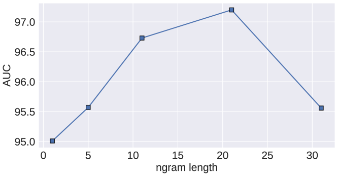
Figure 2: $n$-gram length VS AUC on Cora.

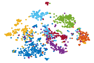
Figure 3: t-SNE visualization on Cora dataset.

5.3 Qualitative Analysis

Embedding visualization.

We employed t-SNE (Maaten and Hinton, 2008) to project the network embeddings for the Cora dataset in a two-dimensional space using GANE-OT, with each node color coded according to its label. As shown in Figure 3, papers clustered together belong to the same category, with the clusters well-separated from each other in the network embedding space. Note that our network embeddings are trained without any label information. Together with the label classification results, this implies our model is capable of extracting meaningful information from both context and network topological.

Attention matrix comparison.

To verify that our OT-based attention mechanism indeed produces sparse attention scores, we visualized the OT attention matrices and compared them with those simarlity-based attention matrices (e.g., WANE). Figure 4 plots one typical example. Our OT solver returns a sparse attention matrix, while dot-product-based WANE attention is effectively dense. This underscores the effectiveness of OT-based attention in terms of noise suppression.

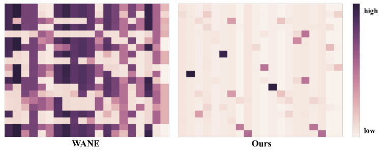
Figure 4: Mutual attention between two nodes in Cora. Left: WANE attention. Right: OT attention (ours).

6 Conclusion

We have proposed a novel and principled mutual-attention framework based on optimal transport (OT). Compared with existing solutions, the attention mechanisms employed by our GANE model enjoys the following benefits: (i) it is naturally sparse and self-normalized, (ii) it is a global sequence matching scheme, and (iii) it can capture long-term interactions between two sentences. These claims are supported by experimental evidence from link prediction and multi-label vertex classification. Looking forward, our attention mechanism can also be applied to tasks such as relational networks (Santoro et al., 2017), natural language inference (MacCartney and Manning, 2009), and QA systems (Zhou et al., 2015).

Appendix A Appendix

A.1 Competing models

A.1.1 Topology only embeddings

Mixed Membership Stochastic Blockmodel (MMB) (Airoldi et al., 2008): a graphical model for relational data, each node randomly select a different ”topic” when forming an edge.

DeepWalk (Perozzi et al., 2014): executes truncated random walks on the graph, and by treating nodes as tokens and random walks as natural language sequences, the node embedding are obtained using the SkipGram model (Mikolov et al., 2013).

Node2vec (Grover and Leskovec, 2016): a variant of DeepWalk by executing biased random walks to explore the neighborhood (e.g., Breadth-first or Depth-first sampling).

Large-scale Information Network Embedding (LINE) (Tang et al., 2015): scalable network embedding scheme via maximizing the joint and conditional likelihoods.

A.2 Joint embedding of topology & text

Naive combination (Tu et al., 2017): direct combination of the structure embedding and text embedding that best predicts edges.

Text-Associated DeepWalk (TADW) (Yang et al., 2015): reformulating embedding as a matrix factorization problem, and fused text-embedding into the solution.

Content-Enhanced Network Embedding (CENE) (Sun et al., 2016): treats texts as a special kind of nodes.

Context-Aware Network Embedding (CANE) (Tu et al., 2017): decompose the embedding into context-free and context-dependent part, use mutual attention to address the context-dependent embedding.

Word-Alignment-based Network Embedding (WANE) (Shen et al., 2018): Using fine-grained alignment to improve context-aware embedding.

Diffusion Maps for Textual network Embedding (DMTE) (Zhang et al., 2018b): using truncated diffusion maps to improve the context-free part embedding in CANE.

Appendix B Complete Link prediction results on Cora and Hepth

The complete results for Cora and Hepth are listed in Tables 5 and 6. Results from models other than GANE are collected from (Tu et al., 2017; Shen et al., 2018; Zhang et al., 2018b). We have also repeated these experiments on our own, the results are consistent with the ones reported. Note that DMTE did not report results on Hepth (Zhang et al., 2018b) .

%Training Edges	15%	25%	35%	45%	55%	65%	75%	85%	95%
MMB	54.7	57.1	59.5	61.9	64.9	67.8	71.1	72.6	75.9
node2vec	55.9	62.4	66.1	75.0	78.7	81.6	85.9	87.3	88.2
LINE	55.0	58.6	66.4	73.0	77.6	82.8	85.6	88.4	89.3
DeepWalk	56.0	63.0	70.2	75.5	80.1	85.2	85.3	87.8	90.3
Naive combination	72.7	82.0	84.9	87.0	88.7	91.9	92.4	93.9	94.0
TADW	86.6	88.2	90.2	90.8	90.0	93.0	91.0	93.4	92.7
CENE	72.1	86.5	84.6	88.1	89.4	89.2	93.9	95.0	95.9
CANE	86.8	91.5	92.2	93.9	94.6	94.9	95.6	96.6	97.7
DMTE	91.3	93.1	93.7	95.0	96.0	97.1	97.4	98.2	98.8
WANE	91.7	93.3	94.1	95.7	96.2	96.9	97.5	98.2	99.1
GANE-OT	92.0	94.4	95.7	96.6	97.3	97.6	98.6	98.8	99.2
GANE-AP	94.0	96.4	97.2	97.4	98.0	98.2	98.8	99.1	99.3

Table 5: AUC scores for link prediction on the Cora dataset.

%Training Edges	15%	25%	35%	45%	55%	65%	75%	85%	95%
MMB	54.6	57.9	57.3	61.6	66.2	68.4	73.6	76.0	80.3
DeepWalk	55.2	66.0	70.0	75.7	81.3	83.3	87.6	88.9	88.0
LINE	53.7	60.4	66.5	73.9	78.5	83.8	87.5	87.7	87.6
node2vec	57.1	63.6	69.9	76.2	84.3	87.3	88.4	89.2	89.2
Naive combination	78.7	82.1	84.7	88.7	88.7	91.8	92.1	92.0	92.7
TADW	87.0	89.5	91.8	90.8	91.1	92.6	93.5	91.9	91.7
CENE	86.2	84.6	89.8	91.2	92.3	91.8	93.2	92.9	93.2
CANE	90.0	91.2	92.0	93.0	94.2	94.6	95.4	95.7	96.3
WANE-ww	92.3	94.1	95.7	96.7	97.5	97.5	97.7	98.2	98.7
DMTE	-	-	-	-	-	-	-	-	-
GANE-OT	93.4	96.2	97.0	97.7	97.9	98.0	98.2	98.6	98.8
GANE-AP	93.8	96.4	97.3	97.9	98.1	98.2	98.4	98.7	98.9

Table 6: AUC scores for link prediction on the Hepth dataset.

B.1 Negative sampling approximation

In this section we provide a quick justification for the negative sampling approximation. To this end, we first briefly review noise contrastive estimation (NCE) and how it connects to maximal likelihood estimation, then we establish the link to negative sampling. Interested readers are referred to Ruder (2016) for a more thorough discussion on this topic.

Noise contrastive estimation.

NCE seeks to learn the parameters of a likelihood model $p_{\Theta}(u|v)$ by optimizing the following discriminative objective:

$$J(\Theta)= \sum_{u_{i}\sim p_{d}}[\log p_{\Theta}(y=1|u_{i},v)-$$

$$K\mathbb{E}_{\tilde{u}^{\prime}\sim p_{n}}[\log p_{\Theta}(y=0|\tilde{u},v)]],$$ (14)

where $y$ is the label of whether $u$ comes from the data distribution $p_{d}$ or the tractable noise distribution $p_{n}$, and $v$ is the context. Using the Monte Carlo estimator for the second term gives us

$$\hat{J}(\Theta)= \sum_{u_{i}\sim p_{d}}[\log p_{\Theta}(y=1|u_{i},v)-$$

$$\sum_{k=1}^{K}[\log p_{\Theta}(y=0|\tilde{u}_{k},v)]],\tilde{u}_{k}\stackrel{{\scriptstyle iid}}{{\sim}}p_{n}.$$ (15)

Since the goal of $J(\Theta)$ is to predict the label of a sample from a mixture distribution with $1/(K+1)$ from $p_{d}$ and $K/(K+1)$ from $p_{n}$, plugging the model likelihood and noise likelihood into the label likelihood gives us

$$p_{\Theta}(y=1;u,v)=\frac{p_{\Theta}(u|v)}{p_{\Theta}(u|v)+Kp_{n}(u|v)},\,$$

$$p_{\Theta}(y=0;u,v)=\frac{Kp_{n}(u|v)}{p_{\Theta}(u|v)+Kp_{n}(u|v)}.$$ (16)

Recall $p_{\Theta}(u|v)$ takes the following softmax form

$$p_{\Theta}(u|v)=\frac{\exp(\langle u,v\rangle)}{Z_{v}(\Theta)},\,Z_{v}(\Theta)=\sum_{u^{\prime}}\exp(\langle u^{\prime},v\rangle).$$ (17)

NCE treats $Z_{v}$ as an learnable parameter and optimized along with $\Theta$. One key observation is that, in practice, one can safely clamp $Z_{v}$ to $1$, and the NCE learned model ($p_{\hat{\Theta}}$) will self-normalize in the sense that $Z_{v}(\hat{\Theta})\approx 1$. As such, one can simply plug $p_{\Theta}(u|v)=\exp(\langle u,v\rangle))$ into the above objective. Another key result is that, as $K\rightarrow\infty$, the gradient of NCE objective recovers the gradient of softmax objective $\log p_{\Theta}(u|v)$ (Dyer, 2014).

Negative sampling as NCE.

If we set $K=\#(\mathcal{V})$ and let $p_{n}(u|v)$ be the uniform distribution on $\mathcal{V}$, we have

$$p_{\Theta}(y=1|u,v)=\sigma(\langle u,v\rangle),$$ (18)

where $\sigma(z)$ is the sigmoid function. Plugging this back to the $\hat{J}(\Theta)$ covers the negative sampling objective Eqn (6) used in the paper. Combined with the discussion above, we know Eqn (6) provides a valid approximation to the $\log$-likelihood in terms of the gradient directions, when $K$ is sufficiently large. In this study, we use $K=1$ negative sample for computational efficiency. Using more samples did not significantly improve our results (data not shown).

B.2 Experiment Setup

We use the same codebase from CANE (Tu et al., 2017). The implementation is based on TensorFlow, all experiments are exectuted on a single NVIDIA TITAN X GPU. We set embedding dimension to $d=100$ for all our experiments. To conduct a fair comparison with the baseline models, we follow the experiment setup from Shen et al. (2018). For all experiments, we set word embedding dimension as 100 trained from scratch. We train the model with Adam optimizer and set learning rate $1e-3$. For GANE-AP model, we use best filte size $1\times 21\times 1$ for convolution from our abalation study.

B.3 Ablation study setup

To test how the $n$-gram length affect our GANE-AP model performance, we re-run our model with different choices of $n$-gram length, namely, the window size in convolutional layer. Each experiment is repeated for $10$ times and we report the averaged results to eliminate statistical fluctuations.

References

- Airoldi et al. (2008) Edoardo M Airoldi, David M Blei, Stephen E Fienberg, and Eric P Xing. 2008. Mixed membership stochastic blockmodels. Journal of Machine Learning Research, 9(Sep):1981–2014.
- Alvarez et al. (2012) Mauricio A Alvarez, Lorenzo Rosasco, Neil D Lawrence, et al. 2012. Kernels for vector-valued functions: A review. Foundations and Trends® in Machine Learning, 4(3):195–266.
- Alvarez-Melis and Jaakkola (2018) David Alvarez-Melis and Tommi S Jaakkola. 2018. Gromov-wasserstein alignment of word embedding spaces. arXiv preprint arXiv:1809.00013.
- Bahdanau et al. (2015) Dzmitry Bahdanau, Kyunghyun Cho, and Yoshua Bengio. 2015. Neural machine translation by jointly learning to align and translate. In ICLR.
- Blei et al. (2003) David M Blei, Andrew Y Ng, and Michael I Jordan. 2003. Latent dirichlet allocation. Journal of machine Learning research, 3(Jan):993–1022.
- Brualdi et al. (1991) Richard A Brualdi, Herbert J Ryser, et al. 1991. Combinatorial matrix theory, volume 39. Springer.
- Chen et al. (2018) Liqun Chen, Shuyang Dai, Chenyang Tao, Dinghan Shen, Zhe Gan, Haichao Zhang, Yizhe Zhang, and Lawrence Carin. 2018. Adversarial text generation via feature-mover’s distance. In NIPS.
- Chen et al. (2019) Liqun Chen, Yizhe Zhang, Ruiyi Zhang, Chenyang Tao, Zhe Gan, Haichao Zhang, Bai Li, Dinghan Shen, Changyou Chen, and Lawrence Carin. 2019. Improving sequence-to-sequence learning via optimal transport. In ICLR.
- Cuturi (2013) Marco Cuturi. 2013. Sinkhorn distances: Lightspeed computation of optimal transport. In NIPS.
- Dyer (2014) Chris Dyer. 2014. Notes on noise contrastive estimation and negative sampling. arXiv preprint arXiv:1410.8251.
- Goldberg and Levy (2014) Yoav Goldberg and Omer Levy. 2014. word2vec explained: deriving mikolov et al.’s negative-sampling word-embedding method. arXiv preprint arXiv:1402.3722.
- Grover and Leskovec (2016) Aditya Grover and Jure Leskovec. 2016. node2vec: Scalable feature learning for networks. In KDD.
- Gulrajani et al. (2017) Ishaan Gulrajani, Faruk Ahmed, Martin Arjovsky, Vincent Dumoulin, and Aaron C Courville. 2017. Improved training of Wasserstein GANs. In NIPS.
- Guo et al. (2018) Han Guo, Ramakanth Pasunuru, and Mohit Bansal. 2018. Soft layer-specific multi-task summarization with entailment and question generation. In ACL.
- Gutmann and Hyvärinen (2010) Michael Gutmann and Aapo Hyvärinen. 2010. Noise-contrastive estimation: A new estimation principle for unnormalized statistical models. In AISTATS.
- He et al. (2016) Kaiming He, Xiangyu Zhang, Shaoqing Ren, and Jian Sun. 2016. Deep residual learning for image recognition. In CVPR.
- Hochreiter et al. (2001) Sepp Hochreiter, Yoshua Bengio, Paolo Frasconi, Jürgen Schmidhuber, et al. 2001. Gradient flow in recurrent nets: the difficulty of learning long-term dependencies.
- Kusner et al. (2015) Matt Kusner, Yu Sun, Nicholas Kolkin, and Kilian Weinberger. 2015. From word embeddings to document distances. In ICML.
- Le and Lauw (2014) Tuan MV Le and Hady W Lauw. 2014. Probabilistic latent document network embedding. In 2014 IEEE International Conference on Data Mining, pages 270–279. IEEE.
- Li et al. (2015) Jiwei Li, Minh-Thang Luong, and Dan Jurafsky. 2015. A hierarchical neural autoencoder for paragraphs and documents. In ACL.
- Liu et al. (2018) Xiaodong Liu, Kevin Duh, and Jianfeng Gao. 2018. Stochastic answer networks for natural language inference. arXiv preprint arXiv:1804.07888.
- Luong et al. (2015) Minh-Thang Luong, Hieu Pham, and Christopher D Manning. 2015. Effective approaches to attention-based neural machine translation. arXiv:1508.04025.
- Maaten and Hinton (2008) Laurens van der Maaten and Geoffrey Hinton. 2008. Visualizing data using t-sne. Journal of machine learning research, 9(Nov):2579–2605.
- MacCartney and Manning (2009) Bill MacCartney and Christopher D Manning. 2009. Natural language inference.
- Malakasiotis and Androutsopoulos (2007) Prodromos Malakasiotis and Ion Androutsopoulos. 2007. Learning textual entailment using svms and string similarity measures. In Proceedings of the ACL-PASCAL Workshop on Textual Entailment and Paraphrasing, pages 42–47.
- Martins and Astudillo (2016) Andre Martins and Ramon Astudillo. 2016. From softmax to sparsemax: A sparse model of attention and multi-label classification. In ICML.
- McCallum et al. (2000) Andrew Kachites McCallum, Kamal Nigam, Jason Rennie, and Kristie Seymore. 2000. Automating the construction of internet portals with machine learning. Information Retrieval, 3(2):127–163.
- Mikolov et al. (2013) Tomas Mikolov, Ilya Sutskever, Kai Chen, Greg S Corrado, and Jeff Dean. 2013. Distributed representations of words and phrases and their compositionality. In NIPS.
- Niculae and Blondel (2017) Vlad Niculae and Mathieu Blondel. 2017. A regularized framework for sparse and structured neural attention. In NIPS.
- Perozzi et al. (2014) Bryan Perozzi, Rami Al-Rfou, and Steven Skiena. 2014. Deepwalk: Online learning of social representations. In KDD.
- Peyré et al. (2017) Gabriel Peyré, Marco Cuturi, et al. 2017. Computational optimal transport. Technical report.
- Ruder (2016) Sebastian Ruder. 2016. On word embeddings - part 2: Approximating the softmax. http://ruder.io/word-embeddings-softmax/.
- Santoro et al. (2017) Adam Santoro, David Raposo, David G Barrett, Mateusz Malinowski, Razvan Pascanu, Peter Battaglia, and Timothy Lillicrap. 2017. A simple neural network module for relational reasoning. In NIPS.
- Santos et al. (2016) Cicero dos Santos, Ming Tan, Bing Xiang, and Bowen Zhou. 2016. Attentive pooling networks. arXiv preprint arXiv:1602.03609.
- Shen et al. (2018) Dinghan Shen, Xinyuan Zhang, Ricardo Henao, and Lawrence Carin. 2018. Improved semantic-aware network embedding with fine-grained word alignment. In EMNLP.
- Sun et al. (2016) Xiaofei Sun, Jiang Guo, Xiao Ding, and Ting Liu. 2016. A general framework for content-enhanced network representation learning. In arXiv preprint arXiv:1610.02906.
- Tang et al. (2015) Jian Tang, Meng Qu, Mingzhe Wang, Ming Zhang, Jun Yan, and Qiaozhu Mei. 2015. LINE: Large-scale information network embedding. In WWW.
- Tang and Liu (2009) Lei Tang and Huan Liu. 2009. Relational learning via latent social dimensions. In KDD.
- Tu et al. (2017) Cunchao Tu, Han Liu, Zhiyuan Liu, and Maosong Sun. 2017. CANE: Context-aware network embedding for relation modeling. In ACL.
- Tu et al. (2016) Cunchao Tu, Weicheng Zhang, Zhiyuan Liu, Maosong Sun, et al. 2016. Max-margin deepwalk: Discriminative learning of network representation. In IJCAI.
- Vaswani et al. (2017) Ashish Vaswani, Noam Shazeer, Niki Parmar, Jakob Uszkoreit, Llion Jones, Aidan N Gomez, Łukasz Kaiser, and Illia Polosukhin. 2017. Attention is all you need. In NIPS.
- Villani (2008) Cédric Villani. 2008. Optimal Transport: Old and New. Springer.
- Wang et al. (2018) Guoyin Wang, Chunyuan Li, Wenlin Wang, Yizhe Zhang, Dinghan Shen, Xinyuan Zhang, Ricardo Henao, and Lawrence Carin. 2018. Joint embedding of words and labels for text classification. In ACL.
- Wang et al. (2017) Xiao Wang, Peng Cui, Jing Wang, Jian Pei, Wenwu Zhu, and Shiqiang Yang. 2017. Community preserving network embedding. In AAAI.
- Weston et al. (2015) Jason Weston, Sumit Chopra, and Antoine Bordes. 2015. Memory networks. In ICLR.
- Xie et al. (2018) Yujia Xie, Xiangfeng Wang, Ruijia Wang, and Hongyuan Zha. 2018. A fast proximal point method for Wasserstein distance. In arXiv:1802.04307.
- Yang et al. (2015) Cheng Yang, Zhiyuan Liu, Deli Zhao, Maosong Sun, and Edward Chang. 2015. Network representation learning with rich text information. In IJCAI.
- Yang et al. (2016) Zichao Yang, Diyi Yang, Chris Dyer, Xiaodong He, Alex Smola, and Eduard Hovy. 2016. Hierarchical attention networks for document classification. In NAACL.
- Zhang et al. (2018a) Daokun Zhang, Jie Yin, Xingquan Zhu, and Chengqi Zhang. 2018a. Network representation learning: A survey. IEEE transactions on Big Data.
- Zhang et al. (2018b) Xinyuan Zhang, Yitong Li, Dinghan Shen, and Lawrence Carin. 2018b. Diffusion maps for textual network embedding. In NIPS.
- Zhou et al. (2015) Guangyou Zhou, Tingting He, Jun Zhao, and Po Hu. 2015. Learning continuous word embedding with metadata for question retrieval in community question answering. In ACL.