Coresets for Data-efficient Training of Machine Learning Models

Abstract

Incremental gradient (IG) methods, such as stochastic gradient descent and its variants are commonly used for large scale optimization in machine learning. Despite the sustained effort to make IG methods more data-efficient, it remains an open question how to select a training data subset that can theoretically and practically perform on par with the full dataset. Here we develop CRAIG, a method to select a weighted subset (or coreset) of training data that closely estimates the full gradient by maximizing a submodular function. We prove that applying IG to this subset is guaranteed to converge to the (near)optimal solution with the same convergence rate as that of IG for convex optimization. As a result, CRAIG achieves a speedup that is inversely proportional to the size of the subset. To our knowledge, this is the first rigorous method for data-efficient training of general machine learning models. Our extensive set of experiments show that CRAIG, while achieving practically the same solution, speeds up various IG methods by up to 6x for logistic regression and 3x for training deep neural networks.

1 Introduction

Mathematical optimization lies at the core of training large-scale machine learning systems, and is now widely used over massive data sets with great practical success, assuming sufficient data resources are available. Achieving this success, however, also requires large amounts of (often GPU) computing, as well as concomitant financial expenditures and energy usage (Strubell et al., 2019). Significantly decreasing these costs without decreasing the learnt system’s resulting accuracy is one of the grand challenges of machine learning and artificial intelligence today (Asi & Duchi, 2019).

Training machine learning models often reduces to optimizing a regularized empirical risk function. Given a convex loss $l$, and a $\mu$-strongly convex regularizer $r$, one aims to find model parameter vector $w_{*}$ over the parameter space $\mathcal{W}$ that minimizes the loss $f$ over the training data $V$:

$$w_{*}\in{\arg\min}_{w\in\mathcal{W}} f(w),\quad f(w):=\sum_{i\in V}f_{i}(w)+r(w),$$

$$f_{i}(w)=l(w,(x_{i},y_{i})),\vspace{-0mm}$$ (1)

where $V=\{1,\dots,n\}$ is an index set of the training data, and functions $f_{i}:\mathbb{R}^{d}\rightarrow\mathbb{R}$ are associated with training examples $(x_{i},y_{i})$, where $x_{i}\in\mathbb{R}^{d}$ is the feature vector, and $y_{i}$ is the point $i$’s label.

Standard Gradient Descent can find the minimizer of this problem, but requires repeated computations of the full gradient $\nabla f(w)$—sum of the gradients over all training data points/functions $i$—and is therefore prohibitive for massive data sets. This issue is further exacerbated in case of deep neural networks where gradient computations (backpropagation) are expensive. Incremental Gradient (IG) methods, such as Stochastic Gradient Descent (SGD) and its accelerated variants, including SGD with momentum (Qian, 1999), Adagrad (Duchi et al., 2011), Adam (Kingma & Ba, 2014), SAGA (Defazio et al., 2014), and SVRG (Johnson & Zhang, 2013) iteratively estimate the gradient on random subsets/batches of training data. While this provides an unbiased estimate of the full gradient, the randomized batches introduce variance in the gradient estimate (Hofmann et al., 2015), and therefore stochastic gradient methods are in general slow to converge (Johnson & Zhang, 2013; Defazio et al., 2014). The majority of the work speeding up IG methods has thus primarily focused on reducing the variance of the gradient estimate (SAGA (Defazio et al., 2014), SVRG (Johnson & Zhang, 2013), Katysha (Allen-Zhu, 2017)) or more carefully selecting the gradient stepsize (Adagrad (Duchi et al., 2011), Adadelta (Zeiler, 2012), Adam (Kingma & Ba, 2014)).

However, the direction that remains largely unexplored is how to carefully select a small subset $S\subseteq V$ of the full training data $V$, so that the model is trained only on the subset $S$ while still (approximately) converging to the globally optimal solution (i.e., the model parameters that would be obtained if training/optimizing on the full $V$). If such a subset $S$ can be quickly found, then this would directly lead to a speedup of $|V|/|S|$ (which can be very large if $|S|\ll|V|$) per epoch of IG.

There are four main challenges in finding such a subset $S$. First is that a guiding principle for selecting $S$ is unclear. For example, selecting training points close to the decision boundary might allow the model to fine tune the decision boundary, while picking the most diverse set of data points would allow the model to get a better sense of the training data distribution. Second is that finding $S$ must be fast, as otherwise identifying the set $S$ may take longer than the actual optimization, and so no overall speed-up would be achieved. Third is that finding a subset $S$ is not enough. One also has to decide on a gradient stepsize for each data point in $S$, as they affect the convergence. And last, while the method might work well empirically on some data sets, one also requires theoretical understanding and mathematical convergence guarantees.

Here we develop Coresets for Accelerating Incremental Gradient descent (CRAIG), for selecting a subset of training data points to speed up training of large machine learning models. Our key idea is to select a weighted subset $S$ of training data $V$ that best approximates the full gradient of $V$. We prove that the subset $S$ that minimizes an upper-bound on the error of estimating the full gradient maximizes a submodular facility location function. Hence, $S$ can be efficiently found using a fast greedy algorithm.

We also provide theoretical analysis of CRAIG and prove its convergence. Most importantly, we show that any incremental gradient method (IG) on $S$ converges in the same number epochs as the same IG would on the full $V$, which means that we obtain a speed-up inversely proportional to the size of $S$. In particular, for a $\mu$-strongly convex risk function and a subset $S$ selected by CRAIG that estimates the full gradient by an error of at most $\epsilon$, we prove that IG on $S$ with diminishing stepsize $\alpha_{k}=\alpha/k^{\tau}$ at epoch $k$ (with $0<\tau<1$ and $0<\alpha$), converges to an $2R\epsilon/\mu^{2}$ neighborhood of the optimal solution at rate $\mathcal{O}(1/\sqrt{k})$. Here, $R=\min\{d_{0},(r\gamma_{\max}C+\epsilon)/\mu\}$ where $d_{0}$ is the initial distance to the optimum, $C$ is an upper-bound on the norm of the gradients, $r=|S|$, and $\gamma_{\max}$ is the largest weight for the elements in the subset obtained by CRAIG. Moreover, we prove that if in addition to the strong convexity, component functions have smooth gradients, IG with the same diminishing step size on subset $S$ converges to a $2\epsilon/\mu$ neighborhood of the optimum solution at rate $\mathcal{O}(1/k^{\tau})$.

The above implies that IG on $S$ converges to the same solution and in the same number of epochs as IG on the full $V$. But because every epoch only uses a subset $S$ of the data, it requires fewer gradient computations and thus leads to a $|V|/|S|$ speedup over traditional IG methods, while still (approximately) converging to the optimal solution. We also note that CRAIG is complementary to various incremental gradient (IG) methods (SGD, SAGA, SVRG, Adam), and such methods can be used on the subset $S$ found by CRAIG.

We also demonstrate the effectiveness of CRAIG via an extensive set of experiments using logistic regression (a convex optimization problem) as well as training deep neural networks (non-convex optimization problems). We show that CRAIG speeds up incremental gradient methods, including SGD, SAGA, and SVRG. In particular, CRAIG while achieving practically the same loss and accuracy as the underlying incremental gradient descent methods, speeds up gradient methods by up to 6x for convex and 3x for non-convex loss functions.

2 Related Work

Convergence of IG methods has been long studied under various conditions (Zhi-Quan & Paul, 1994; Mangasariany & Solodovy, 1994; Bertsekas, 1996; Solodov, 1998; Tseng, 1998), however IG’s convergence rate has been characterized only more recently (see (Bertsekas, 2015b) for a survey). In particular, (Nedić & Bertsekas, 2001) provides a $\mathcal{O}(1/\sqrt{k})$ convergence rate for diminishing stepsizes $\alpha_{k}$ per epoch $k$ under a strong convexity assumption, and (Gürbüzbalaban et al., 2015) proves a $\mathcal{O}(1/k^{\tau})$ convergence rate with diminishing stepsizes $\alpha_{k}=\Theta(1/k^{\tau})$ for $\tau\in(0,1]$ under an additional smoothness assumption for the components. While these works provide convergence on the full dataset, our analysis provides the same convergence rates on subsets obtained by CRAIG.

Techniques for speeding up SGD, are mostly focused on variance reduction techniques (Roux et al., 2012; Shalev-Shwartz & Zhang, 2013; Johnson & Zhang, 2013; Hofmann et al., 2015; Allen-Zhu et al., 2016), and accelerated gradient methods when the regularization parameter is small (Frostig et al., 2015; Lin et al., 2015; Xiao & Zhang, 2014). Very recently, (Hofmann et al., 2015; Allen-Zhu et al., 2016) exploited neighborhood structure to further reduce the variance of stochastic gradient descent and improve its running time. Our CRAIG method and analysis are complementary to variance reduction and accelerated methods. CRAIG can be applied to all these methods as well to speed them up.

Coresets are weighted subsets of the data, which guarantee that models fitting the coreset also provide a good fit for the original data. Coreset construction methods traditionally perform importance sampling with respect to sensitivity score, to provide high-probability solutions (Har-Peled & Mazumdar, 2004; Lucic et al., 2017; Cohen et al., 2017) for a particular problem, such as $k$-means and $k$-median clustering (Har-Peled & Mazumdar, 2004), naïve Bayes and nearest-neighbors (Wei et al., 2015), mixture models (Lucic et al., 2017), low rank approximation (Cohen et al., 2017), spectral approximation (Agarwal et al., 2004; Li et al., 2013), Nystrom methods (Agarwal et al., 2004; Musco & Musco, 2017), and Bayesian inference (Campbell & Broderick, 2018). Unlike existing coreset construction algorithms, our method is not problem specific and can be applied for training general machine learning models.

3 Coresets for Accelerating Incremental Gradient Descent (CRAIG)

We proceed as follows: First, we define an objective function $L$ for selecting an optimal set $S$ of size $r$ that best approximates the gradient of the full training dataset $V$ of size $n$. Then, we show that $L$ can be turned into a submodular function $F$ and thus $S$ can be efficiently found using a fast greedy algorithm. Crucially, we also show that for convex loss functions the approximation error between the estimated and the true gradient can be efficiently minimized in a way that is independent of the actual optimization procedure. Thus, CRAIG can simply be used as a preprocessing step before the actual optimization starts.

Incremental gradient methods aim at estimating the full gradient $\nabla f(w)$ over $V$ by iteratively making a step based on the gradient of every function $f_{i}$. Our key idea in CRAIG is that if we can find a small subset $S$ such that the weighted sum of the gradients of its elements closely approximates the full gradient over $V$, we can apply IG only to the set $S$ (with stepsizes equal to the weight of the elements in $S$), and we should still converge to the (approximately) optimal solution, but much faster.

Specifically, our goal in CRAIG is to find the smallest subset $S\subseteq V$ and corresponding per-element stepsizes $\gamma_{j}>0$ that approximate the full gradient with an error at most $\epsilon>0$ for all the possible values of the optimization parameters $w\in\mathcal{W}$.

$$S^{*}= {\arg\min}_{S\subseteq V,\gamma_{j}\geq 0~{}\forall j}|S|,\;\;\text{s.t.}$$

$$\max_{w\in\mathcal{W}}\|\sum_{i\in V}\nabla f_{i}(w)-\sum_{j\in S}\gamma_{j}\nabla f_{j}(w)\|\leq\epsilon.$$ (2)

Given such an $S^{*}$ and associated weights $\{\gamma\}_{j}$, we are guaranteed that gradient updates on $S^{*}$ will be similar to the gradient updates on $V$ regardless of the value of $w$.

Unfortunately, directly solving the above optimization problem is not feasible, due to two problems. Problem 1: Eq. (3) requires us to calculate the gradient of all the functions $f_{i}$ over the entire space $\mathcal{W}$, which is too expensive and would not lead to overall speedup. In other words, it would appear that solving for $S^{*}$ is as difficult as solving Eq. (1), as it involves calculating $\sum_{i\in V}\nabla f_{i}(w)$ for various $w\in\mathcal{W}$. And Problem 2: even if calculating the normed difference between the gradients in Eq. (3) would be fast, as we discuss later finding the optimal subset $S^{*}$ in NP-hard. In the following, we address the above two challenges and discuss how we can quickly find a near-optimal subset $S$.

3.1 Upper-bound on the Estimation Error

We first address Problem 1, i.e., how to quickly estimate the error/discrepancy of the weighted sum of gradients of functions $f_{j}$ associate with data points $j\in S$, vs the full gradient, for every $w\in\mathcal{W}$.

Let $S$ be a subset of $r$ data points. Furthermore, assume that there is a mapping $\varsigma_{w}:V\rightarrow S$ that for every $w\in\mathcal{W}$ assigns every data point $i\in V$ to one of the elements $j$ in $S$, i.e., ${\varsigma_{w}(i)}={j}\in S$. Let $C_{j}=\{i\in[n]|{\varsigma(i)}={j}\}\subseteq V$ be the set of data points that are assigned to ${j}\in S$, and $\gamma_{j}=|C_{j}|$ be the number of such data points. Hence, $\{C_{j}\}_{j=1}^{r}$ form a partition of $V$. Then, for any arbitrary (single) $w\in\mathcal{W}$ we can write

$$\!\!\sum_{i\in V}\!\nabla f_{i}(w) \!=\!\sum_{i\in V}\!\big{(}\nabla f_{i}(w)\!-\!\nabla f_{\varsigma_{w}(i)}(w)\!+\!\nabla f_{\varsigma_{w}(i)}(w)\big{)}\!\!$$ (3)

$$=\sum_{i\in V}\big{(} \nabla f_{i}(w)-\nabla f_{\varsigma_{w}(i)}(w)\big{)}+\sum_{j\in S}\gamma_{j}\nabla f_{j}(w).\vspace{-2mm}$$ (4)

Subtracting and then taking the norm of the both sides, we get an upper bound on the error of estimating the full gradient with the weighted sum of the gradients of the functions $\!f_{j}$ for $\!j\!\in\!S$. I.e.,

$$\vspace{-2mm}\|\sum_{i\in V}\nabla f_{i}(w)-\sum_{j\in S} \gamma_{j}\nabla f_{j}(w)\|\leq$$

$$\sum_{i\in V}\|\nabla f_{i}(w)-\nabla f_{\varsigma_{w}(i)}(w)\|,\vspace{-2mm}$$ (5)

where the inequality follows from the triangle inequality. The upper-bound in Eq. (5) is minimized when $\varsigma_{w}$ assigns every $i\in V$ to an element in $S$ with most gradient similarity at $w$, or minimum Euclidean distance between the gradient vectors at $w$. That is: $\!\varsigma_{w}(i)\in{\arg\min}_{j\in S}\|\nabla f_{i}(w)-\nabla f_{j}(w)\|$. Hence,

$$\min_{S\subseteq V}\|\sum_{i\in V}\nabla f_{i}(w)- \sum_{j\in S}\gamma_{j}\nabla f_{j}(w)\|\leq$$

$$\sum_{i\in V}\min_{j\in S}\|\nabla f_{i}(w)-\nabla f_{j}(w)\|.\vspace{-2mm}$$ (6)

The right hand side of Eq. (6) is minimized when $S$ is the set of $r$ medoids (exemplars) (Kaufman et al., 1987) for all the components in the gradient space.

So far, we considered upper-bounding the gradient estimation error at a particular $w\in\mathcal{W}$. To bound the estimation error for all $w\in\mathcal{W}$, we consider a worst-case approximation of the estimation error over the entire parameter space $\mathcal{W}$. Formally, we define a distance metric $d_{ij}$ between gradients of $f_{i}$ and $f_{j}$ as the maximum normed difference between $\nabla f_{i}(w)$ and $\nabla f_{j}(w)$ over all $w\in\mathcal{W}$:

$$d_{ij}\triangleq\max_{w\in\mathcal{W}}\|\nabla f_{i}(w)-\nabla f_{j}(w)\|.$$ (7)

Thus, by solving the following minimization problem, we obtain the smallest weighted subset $S^{*}$ that approximates the full gradient by an error of at most $\epsilon$ for all $w\in\mathcal{W}$:

$$\vspace{-1mm}S^{*}\!\!=\!{\arg\min}_{S\subseteq V}|S|,\quad\text{s.t.}\quad L(S)\triangleq\sum_{i\in V}\min_{j\in S}d_{ij}\!\leq\!\epsilon.\vspace{-1mm}$$ (8)

Note that Eq. (8) requires that the gradient error is bounded over $\!\mathcal{W}$. However, we show (Appendix B.1) for several classes of convex problems, including linear regression, ridge regression, logistic regression, and regularized support vector machines (SVMs), the normed gradient difference between data points can be efficiently boundedly approximated by (Allen-Zhu et al., 2016; Hofmann et al., 2015):

$$\vspace{-2mm}\forall w,i, j\quad\|\nabla f_{i}(w)-\nabla f_{j}(w)\|\leq d_{ij}\leq$$

$$\max_{w\in\mathcal{W}}\mathcal{O}(\|w\|)\cdot\|x_{i}-x_{j}\|=\text{const.}~{}\|x_{i}-x_{j}\|.\vspace{-1mm}$$ (9)

Note when $\|w\|$ is bounded for all $w\in\mathcal{W}$, i.e., $\max_{w\in\mathcal{W}}\mathcal{O}(\|w\|)<\infty$, upper-bounds on the Euclidean distances between the gradients can be pre-computed. This is crucial, because it means that estimation error of the full gradient can be efficiently bounded independent of the actual optimization problem (i.e., point $w$). Thus, these upper-bounds can be computed only once as a pre-processing step before any training takes place, and then used to find the subset $S$ by solving the optimization problem (8). We address upper-bounding the normed difference between gradients for deep models in Section 3.4.

3.2 The CRAIG Algorithm

Optimization problem (8) produces a subset $S$ of elements with their associated weights $\{\gamma\}_{j\in S}$ or per-element stepsizes that closely approximates the full gradient. Here, we show how to efficiently approximately solve the above optimization problem to find a near-optimal subset $S$.

The optimization problem (8) is NP-hard as it involves calculating the value of $L(S)$ for all the $2^{|V|}$ subsets $S\subseteq V$. We show, however, that we can transform it into a submodular set cover problem, that can be efficiently approximated.

Formally, $F$ is submodular if $F(S\cup\{e\})-F(S)\geq F(T\cup\{e\})-F(T),$ for any $S\subseteq T\subseteq V$ and $e\in V\setminus T$. We denote the marginal utility of an element $e$ w.r.t. a subset $S$ as $F(e|S)=F(S\cup\{e\})-F(S)$. Function $F$ is called monotone if $F(e|S)\geq 0$ for any $e\!\in\!V\!\setminus\!S$ and $S\subseteq V$. The submodular cover problem is defined as finding the smallest set $S$ that achieves utility $\rho$. Precisely,

$$S^{*}={\arg\min}_{S\subseteq V}|S|,\quad\text{s. t.}\quad F(S)\geq\rho.\vspace{-1mm}$$ (10)

Although finding $S^{*}$ is NP-hard since it captures such well-known NP-hard problems such as Minimum Vertex Cover, for many classes of submodular functions, a simple greedy algorithm is known to be very effective (Nemhauser et al., 1978; Wolsey, 1982). The greedy algorithm starts with the empty set $S_{0}=\emptyset$, and at each iteration $i$, it chooses an element $e\in V$ that maximizes $F(e|S_{i-1})$, i.e., $S_{i}=S_{i-1}\cup\{{\arg\max}_{e\in V}F(e|S_{i-1})\}.$ Greedy gives us a logarithmic approximation, i.e. $|S|\leq\big{(}1+\ln(\max_{e}F(e|\emptyset))\big{)}|S^{*}|$ (Wolsey, 1982). The computational complexity of the greedy algorithm is $\mathcal{O}(|V|\cdot|S|)$. However, its running time can be reduced to $\mathcal{O}(|V|)$ using stochastic algorithms (Mirzasoleiman et al., 2015a) and further improved using lazy evaluation (Minoux, 1978), and distributed implementations (Mirzasoleiman et al., 2015b, 2016). Given a subset $S\subseteq V$, the facility location function quantifies the coverage of the whole data set $V$ by the subset $S$ by summing the similarities between every $i\in V$ and its closest element $j\in S$. Formally, facility location is defined as $F_{fl}(S)=\sum_{i\in V}\max_{j\in S}s_{i,j}$, where $s_{i,j}$ is the similarity between $i,j\in V$. The facility location function has been used in various summarization applications (Lin et al., 2009; Lin & Bilmes, 2012). By introducing an auxiliary element $s_{0}$ we can turn $L(S)$ in Eq. (8) into a monotone submodular facility location function,

$$F(S)=L(\{s_{0}\})-L(S\cup\{s_{0}\}),\vspace{-1mm}$$ (11)

where $L(\{s_{0}\})$ is a constant. In words, $F$ measures the decrease in the estimation error associated with the set $S$ versus the estimation error associated with just the auxiliary element. For a suitable choice of $s_{0}$, maximizing $F$ is equivalent to minimizing $L$. Therefore, we apply the greedy algorithm to approximately solve the following problem to get the subset $S$ defined in Eq. (8):

$$S^{*}={\arg\min}_{S\subseteq V}|S|,\quad\text{s.t.}\quad F(S)\geq L(\{s_{0}\})-\epsilon.$$ (12)

At every step, the greedy algorithm selects an element that reduces the upper bound on the estimation error the most. In fact, the size of the smallest subset $S$ that estimates the full gradient by an error of at most $\epsilon$ depends on the structural properties of the data. Intuitively, as long as the marginal gains of facility location are considerably large, we need more elements to improve our estimation of the full gradient. Having found $S$, the weight $\gamma_{j}$ of every element $j\in S$ is the number of components that are closest to it in the gradient space, and are used as stepsize of element $j\in S$ during IG. The pseudocode for CRAIG is outlined in Algorithm 1.

Notice that CRAIG creates subset $S$ incrementally one element at a time, which produces a natural order to the elements in $S$. Adding the element with largest marginal gain $j\in{\arg\max}_{e\in V}F(e|S_{i-1})$ improves our estimation from the full gradient by an amount bounded by the marginal gain. At every step $i$, we have $F(S_{i})\geq(1-e^{-i/|S|})F(S^{*})$. Hence, for a greedily ordered subset $S=\{s_{1},\cdots,s_{k}\}$, we have

$$\|\sum_{i\in V}\nabla f_{i}(w)-\sum_{j=1}^{k}\gamma_{s_{j}}\nabla f_{s_{j}}(w)\|\leq c-(1-e^{-j/k})L(S^{*}),\vspace{-1mm}$$ (13)

where $c$ is a constant. Intuitively, the first elements of the ordering contribute the most to provide a close approximation of the full gradient and the rest of the elements further refine the approximation. Hence, the first incremental gradient updates gets us close to $w_{*}$, and the rest of the updates further refine the solution.

0:  Set of component functions $f_{i}$ for $i\in V=[n]\}$.

0:  Subset $S\subseteq V$ with corresponding per-element stepsizes $\{\gamma\}_{j\in S}$.

1:  $S_{0}\leftarrow\emptyset,s_{0}=0,i=0.$

2:  while $F(S)<L(\{s_{0}\})-\epsilon$ do

3:     $j\in{\arg\max}_{e\in V\setminus S_{i-1}}F(e|S_{i-1})$

4:     $S_{i}=S_{i-1}\cup\{j\}$

5:     $i=i+1$

6:  end while

7:  for $j=1$ to $|S|$ do

8:     $\gamma_{j}=\sum_{i\in V}\mathbb{I}\big{[}j={\arg\min}_{s\in S}{\max_{w\in\mathcal{W}}}\|\nabla f_{i}(w)-\nabla f_{s}(w)\|\big{]}$

9:  end for

Algorithm 1 CRAIG (CoResets for Accelerating Incremental Gradient descent)

3.3 CRAIG with Limited Budget

In practice, we often have a limited budget in terms of time or computational resources, and we are interested to find a near-optimal subset of size $r$ that best approximates the full gradient. This problem can be formulated as a submodular maximization problem which is dual to the submodular cover problem (12):

$$S^{*}\in{\arg\max}_{S\subseteq V}F(S),\quad\text{s.t.}\quad|S|\leq r.$$ (14)

For the above submodular maximization problem, the greedy algorithm discussed in Section 3.2 provides a $(1-1/e)$-approximation to the optimal solution. For a subset $S$ of size at most $r$ obtained by the greedy algorithm, we can calculate the value of $\epsilon$ as follows:

$$\epsilon\leq F(S)-L(\{s_{0}\}).$$ (15)

We use this formulation in our experiments in Section 5.

3.4 Application of CRAIG to Deep Networks

As discussed, CRAIG selects a subset that closely approximates the full gradient, and hence can be also applied for speeding up training deep networks. The challenge here is that we cannot use inequality (3.1) to bound the normed difference between gradients for all $w\in\mathcal{W}$ and find the subset as a preprocessing step.

However, for deep neural networks, the variation of the gradient norms is mostly captured by the gradient of the loss w.r.t. the input to the last layer [Section 3.2 of (Katharopoulos & Fleuret, 2018)]. We show (Appendix B.1) that the normed gradient difference between data points can be efficiently bounded approximately by

$$\|\nabla f_{i}(w)-\nabla f_{j}(w)\|\leq$$ (16)

$$c_{1}\|\Sigma^{\prime}_{L}(z_{i}^{(L)}) \nabla f_{i}^{(L)}(w)-\Sigma^{\prime}_{L}(z_{j}^{(L)})\nabla f_{j}^{(L)}(w)\|+c_{2},$$

where $\Sigma^{\prime}_{L}(z_{i}^{(L)})\nabla f_{i}^{(L)}(w)$ is gradient of the loss w.r.t. the input to the last layer for data point $i$, and $c_{1},c_{2}$ are constants. The above upper-bound depends on parameter vector $w$ which changes during the training process. Thus, we need to use CRAIG to update the subset $S$ after a number of parameter updates.

The above upper-bound is often only slightly more expensive than calculating the loss. For example, in cases where we have cross entropy loss with soft-max as the last layer, the gradient of the loss w.r.t. the $i$-th input to the soft-max is simply $p_{i}-y_{i}$, where $p_{i}$ are logits (dimension $p\!-\!1$ for $p$ classes) and $y$ is the one-hot encoded label. In this case, CRAIG does not need any backward pass or extra storage. Note that, although CRAIG needs an additional $\mathcal{O}(|V|\cdot|S|)$ complexity (or $\mathcal{O}(|V|)$ using stochastic greedy) to find the subset $S$ at the beginning of every epoch, this complexity does not involve any (exact) gradient calculations and is negligible compared to the cost of backpropagations performed during the epoch. Hence, as we show in the experiments CRAIG is practical and scalable.

4 Convergence Rate Analysis of CRAIG

The idea of CRAIG is to selects a subset that closely approximates the full gradient, and hence can be applied to speed up most IG variants as we show in our experiments. Here, we briefly introduce the original IG method, and then prove the convergence rate of IG applied to CRAIG subsets.

4.1 Incremental Gradient Methods (IG)

Incremental gradient (IG) methods are core algorithms for solving Problem (1) and are widely used and studied. IG aims at approximating the standard gradient method by sequentially stepping along the gradient of the component functions $f_{i}$ in a cyclic order. Starting from an initial point $w_{0}^{1}\in\mathbb{R}^{d}$, it makes $k$ passes over all the $n$ components. At every epoch $k\geq 1$, it iteratively updates $w_{i-1}^{k}$ based on the gradient of $f_{i}$ for $i=1,\cdots,n$ using stepsize $\alpha_{k}>0$. I.e.,

$$\vspace{-1mm}w_{i}^{k}=w_{i-1}^{k}-\alpha_{k}\nabla f_{i}(w_{i-1}^{k}),\quad\quad i=1,2,\cdots,n,$$ (17)

with the convention that $w_{0}^{k+1}=w_{n}^{k}$. Note that for a closed and convex subset $\mathcal{W}$ of $\mathbb{R}^{d}$, the results can be projected onto $\mathcal{W}$, and the update rule becomes

$$w_{i}^{k}=P_{\mathcal{W}}(w_{i-1}^{k}-\alpha_{k}\nabla f_{i}(w_{i-1}^{k})),\quad\quad i=1,2,\cdots,n,$$ (18)

where $P_{\mathcal{W}}$ denotes projection on the set $\mathcal{W}\subset\mathbb{R}^{d}$.

IG with diminishing stepsizes converges at rate $\mathcal{O}(1/\sqrt{k})$ for strongly convex sum function (Nedić & Bertsekas, 2001). If in addition to the strong convexity of the sum function, every component function $f_{i}$ is smooth, IG with diminishing stepsizes $\alpha_{k}=\Theta({1}/{k^{s}}),s\in(0,1]$ converges at rate $\mathcal{O}(1/k^{s})$ (Gürbüzbalaban et al., 2015).

The convergence rate analysis of IG is valid regardless of order of processing the elements. However, in practice, the convergence rate of IG is known to be quite sensitive to the order of processing the functions (Bertsekas, 2015a; Gurbuzbalaban et al., 2017). If problem-specific knowledge can be used to find a favorable order $\sigma$ (defined as a permutation $\{\sigma_{1},\cdots,\sigma_{n}\}$ of $\{1,2,...,n\}$), IG can be updated to process the functions according to this order, i.e.,

$$w_{i}^{k}=w_{i-1}^{k}-\alpha_{k}\nabla f_{\sigma_{i}}(w_{i-1}^{k}),\quad\quad i=1,2,\cdots,n.$$ (19)

In general a favorable order is not known in advance. A common approach is sampling the function indices with replacement from the set $\{1,2,\cdots,n\}$, which is called the Stochastic Gradient Descent (SGD) method.

4.2 Convergence Rate of IG on CRAIG Subsets

Next we analyze the convergence rate of IG applied to the weighted subset $S$ found by CRAIG. Note that CRAIG finds $S$ by greedily minimizing (12) (or maximizing (14)). Therefore, $S$ is a near-optimal solution of problem (3) and estimates the full gradient by an error of at most $\epsilon$, i.e., $\max_{w\in\mathcal{W}}\|\sum_{i\in V}\nabla f_{i}(w)-\sum_{j\in S}\gamma_{j}\nabla f_{j}(w)\|\leq\epsilon$.

Here, we show that (1) applying IG to $S$ converges to a close neighborhood of the optimal solution and that (2) this convergence happens at the same rate (same number of epochs) as IG on the full data. Formally, every step of IG on the subset becomes

$$w_{i}^{k}=w_{i-1}^{k}-\alpha_{k}\gamma_{s_{\sigma_{i}}}\nabla f_{s_{\sigma_{i}}}(w_{i-1}^{k}),\quad i=1,2,\cdots,r,$$

$$\quad\quad s_{i}\in S,\quad|S|=r.$$ (20)

Here, $\sigma$ is a permutation of $\{1,2,\cdots,r\}$, and the per-element stepsize $\gamma_{s_{i}}$ for every function $f_{s_{i}}$ is the weight of the element $s_{i}\in S$ and is fixed for all epochs.

4.3 Convergence for Strongly Convex $f$

We first provide the convergence analysis for the case where the function $f$ in Problem (1) is strongly convex, i.e. $\forall w,w^{\prime}\in\mathbb{R}^{d}$ we have $f(w)\geq f(w^{\prime})+\langle\nabla f(w^{\prime}),w-w^{\prime}\rangle+\frac{\mu}{2}\|w^{\prime}-w\|^{2}$.

Theorem 1.

Assume that $f$ is strongly convex, and $S$ is a weighted subset of size $r$ obtained by CRAIG that estimates the full gradient by an error of at most $\epsilon$, i.e., $\max_{w\in\mathcal{W}}\|\sum_{i\in V}\nabla f_{i}(w)-\sum_{j\in S}\gamma_{j}\nabla f_{j}(w)\|\leq\epsilon$. Then for the iterates $\{w_{k}\!=\!w_{0}^{k}\}$ generated by applying IG to $S$ with per-epoch stepsize $\alpha_{k}=\alpha/k^{\tau}$ with $\alpha>0$ and $\tau\in[0,1]$, we have

• if $\tau=1$, then $\|w_{k}-w_{*}\|^{2}\!\leq\!2\epsilon R/\mu^{2}\!+\alpha r^{2}\gamma_{\max}^{2}C^{2}\!/k\mu$,

• if $0<\tau<1$, then $\|w_{k}-w_{*}\|^{2}\!\leq\!2\epsilon R/\mu^{2}$, for $k\rightarrow\infty$

• if $\tau=0$, then $\|w_{k}-w_{*}\|^{2}\leq(1-\alpha\mu)^{k+1}\|w_{0}-w_{*}\|^{2}+2\epsilon R/\mu^{2}+\alpha r^{2}\gamma_{\max}^{2}C^{2}/\mu,$

where $C$ is an upper-bound on the norm of the component function gradients, i.e. $\max_{i\in V}\sup_{w\in\mathcal{W}}\|\nabla f_{i}(w)\|\leq C$, $\gamma_{\max}=\max_{j\in S}\gamma_{j}$ is the largest per-element step size, and $R=\min\{d_{0},(r\gamma_{\max}C+\epsilon)/\mu\}$, where $d_{0}=\|w_{0}-w_{*}\|$ is the initial distance to the optimum $w_{*}$.

All the proofs can be found in the Appendix. The above theorem shows that IG on $S$ converges at the same rate $\mathcal{O}(1/\sqrt{k})$ of IG on the entire data set $V$. However, compared to IG on $V$, the $|V|/|S|$ speedup of IG on $S$ comes at the price of getting an extra error term, $2\epsilon R/\mu^{2}$.

(a) SGD

(b) SAGA

(c) SVRG

Figure 1: Loss residual and error rate of SGD, SVRG, SAGA for Logistic Regression on Covtype data set with 581,012 data points. We compare CRAIG (10% selected subset) (blue) vs. 10% random subset (green) vs. entire data set (orange). CRAIG gives the average speedup of 3x for achieving similar loss residual and error rate across the three optimization methods.

4.4 Convergence for Smooth and Strongly Convex $f$

If in addition to strong convexity of the expected risk, each component function has a Lipschitz gradient, i.e. $\forall w\in\mathcal{W},i\in[n]$ we have $\|\nabla f_{i}(w)-\nabla f_{i}(w^{\prime})\|\leq\!\beta_{i}\|w-w^{\prime}\|$, then we get the following results about the iterates generated by applying IG to the weighted subset $S$ returned by CRAIG.

Theorem 2.

Assume that $f$ is strongly convex and let $f_{i}(w),i=1,2,\cdots,n$ be convex and twice continuously differentiable component functions with Lipschitz gradients on $\mathcal{W}$. Supposed that $S$ is a weighted subset of size $r$ obtained by CRAIG that estimates the full gradient by an error of at most $\epsilon$, i.e., $\max_{w\in\mathcal{W}}\|\sum_{i\in V}\nabla f_{i}(w)-\sum_{j\in S}\gamma_{j}\nabla f_{j}(w)\|\leq\epsilon$. Then for the iterates $\{w_{k}=w_{0}^{k}\}$ generated by applying IG to $S$ with per-epoch stepsize $\alpha_{k}=\alpha/k^{\tau}$ with $\alpha>0$ and $\tau\in[0,1]$, we have

• if $\tau=1$, then $\|w_{k}-w_{*}\|\leq 2\epsilon/\mu+\alpha\beta Cr\gamma_{\max}^{2}/k\mu$,

• if $0<\tau<1$, then $\|w_{k}-w_{*}\|\leq 2\epsilon/\mu$, for $k\rightarrow\infty$

• if $\tau=0$, then $\|w_{k}-w_{*}\|\leq(1-\alpha\mu)^{k}\|w_{0}-w_{*}\|+2\epsilon/\mu+\alpha\beta Cr\gamma_{\max}^{2}/\mu$,

where $\beta=\sum_{i=1}^{n}\beta_{i}$ is the sum of gradient Lipschitz constants of the component functions.

The above theorem shows that for $\tau>0$, IG applied to $S$ converges to a $2\epsilon/\mu$ neighborhood of the optimal solution, with a rate of $\mathcal{O}(1/k^{\tau})$ which is the same convergence rate for IG on the entire data set $V$. As shown in our experiments, in real data sets small weighted subsets constructed by CRAIG provide a close approximation to the full gradient. Hence, applying IG to the weighted subsets returned by CRAIG provides a solution of the same or higher quality compared to the solution obtained by applying IG to the whole data set, in a considerably shorter amount of time.

5 Experiments

In our experimental evaluation we wish to address the following questions: (1) How do loss and accuracy of IG applied to the subsets returned by CRAIG compare to loss and accuracy of IG applied to the entire data? (2) How small is the size of the subsets that we can select with CRAIG and still get a comparable performance to IG applied to the entire data? And (3) How well does CRAIG scale to large data sets, and extends to non-convex problems? In our experiments, we report the run-time as the wall-clock time for subset selection with CRAIG, plus minimizing the loss using IG or other optimizers with the specified learning rates. For the classification problems, we separately select subsets from each class while maintaining the class ratios in the whole data, and apply IG to the union of the subsets. Note that the upper bounds on the gradient differences derived in Appendix B.1 only hold for points with similar labels. Thus, theoretically we need to select subsets separately. For neural networks, we observed that separately selecting subsets from each class helps the performance. We separately tune each method so that it performs at its best.

5.1 Convex Experiments

In our convex experiments, we apply CRAIG to SGD, as well as SVRG (Johnson & Zhang, 2013), and SAGA (Defazio et al., 2014). We apply L2-regularized logistic regression: $f_{i}(x)=\ln(1+\exp(-w^{T}x_{i}y_{i}))+0.5\lambda w^{T}w$ to classify the following two datasets from LIBSVM: (1) covtype.binary including 581,012 data points of 54 dimensions, and (2) Ijcnn1 including 49,990 training and 91,701 test data points of 22 dimensions. As covtype does not come with labeled test data, we randomly split the training data into halves to make the training/test split (training and set sets are consistent for different methods).

For the convex experiments, we tuned the learning rate for each method (including the random baseline) by preferring smaller training loss from a large number of parameter combinations for two types of learning scheduling: exponential decay $\alpha_{k}=\alpha_{0}b^{k}$ and $k$-inverse $\alpha_{k}=\alpha_{0}(1+bk)^{-1}$ with parameters $\alpha_{0}$ and $b$ to adjust. For convergence of IG to $2\epsilon/\mu$ neighborhood of the optimal solution, we require that $\sum_{k=0}^{\infty}\alpha_{k}=\infty$, and $\sum_{k=0}^{\infty}\alpha^{2}_{k}=0$ (Nedić & Bertsekas, 2001). Hence, while the convergence of exponentially decaying learning rate is not theoretically guaranteed, it often worked better in our experiments. Furthermore, following (Johnson & Zhang, 2013) we set $\lambda$ to $10^{-5}$.

(a) Covtype

(b) Ijcnn1

Figure 2: Normed difference between the full gradient, the gradient of the subset found by CRAIG (Eq. 3), and the theoretical upper-bound $\epsilon$ (Eq. 8). The values are normalized by the largest full gradient norm. The transparent green lines demonstrate various random subsets, and the opaque green line shows their average.

Figure 3: Training loss residual for SGD applied to subsets of size $10\%,20\%,\cdots,90\%$ found by CRAIG vs. random subsets of the same size from Ijcnn1. We get 5.6x speedup from applying SGD to subset of size 30% compared to the entire dataset.

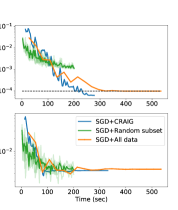
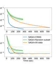
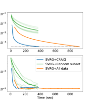
CRAIG effectively minimizes the loss. Figure 1(top) compares training loss residual of SGD, SVRG, and SAGA on the 10% CRAIG set (blue), 10% random set (green), and the full dataset (orange). CRAIG effectively minimizes the training data loss (blue line) and achieves the same minimum as the entire dataset training (orange line) but much faster. Also notice that training on the random 10% subset of the data does not effectively minimize the training loss.

Figure 4: Test accuracy and training loss of SGD applied to subsets found by CRAIG vs. random subsets on MNIST with a 2-layer neural network. CRAIG provides 2x to 3x speedup and a better generalization performance.

CRAIG has a good generalization performance. Figure 1(bottom) shows the test error rate of models trained on CRAIG vs. random vs. the full data. Notice that training on CRAIG subsets achieves the same generalization performance (test error rate) as training on the full data.

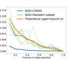
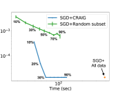
CRAIG achieves significant speedup. Figure 1 also shows that CRAIG achieves a similar training loss (top) and test error rate (bottom) as training on the entire set, but much faster. In particular, we obtain a speedup of 2.75x, 4.5x, 2.5x from applying IG, SVRG and SAGA on the subsets of size 10% from covtype obtained by CRAIG. Furthermore, Figure 3 compares the speedup achieved by CRAIG to reach a similar loss residual as that of SGD for subsets of size $10\%,20\%,\cdots,90\%$ of Ijcnn1. We get a 5.6x speedup by applying SGD to subsets of size 30% obtained by CRAIG.

CRAIG gradient approximation is accurate. Figure 2 demonstrates the norm of the difference between the weighted gradient of the subset found by CRAIG and the full gradient compared to the theoretical upper-bound $\epsilon$ specified in Eq. (8). The gradient difference is calculated by sampling the full gradient at various points in the parameter space. Gradient differences are then normalized by the largest norm of the sampled full gradients. The figure also compares the normed gradient difference between gradients of several random subsets $S$ where each data point is weighted by $|V|/|S|$. Notice that CRAIG’s gradient estimate is more accurate than the gradient estimate obtained by the same-size random subset of points (which is how methods like SGD approximate the gradient). This demonstrates that our gradient approximation in Eq. (8) is reliable in practice.

5.2 Non-convex Experiments

Our non-convex experiments involve applying CRAIG to train the following two neural networks: (1) Our smaller network is a fully-connected hidden layer of 100 nodes and ten softmax output nodes; sigmoid activation and L2 regularization with $\lambda=10^{-4}$ and mini-batches of size 10 on MNIST dataset of handwritten digits containing 60,000 training and 10,000 test images. (2) Our large neural network is ResNet-20 for CIFAR10 with convolution, average pooling and dense layers with softmax outputs and L2 regularization with $\lambda=10^{-4}$. CIFAR 10 includes 50,000 training and 10,000 test images from 10 classes, and we used mini-batches of size 128. Both MNIST and CIFAR10 data sets are normalized into [0, 1] by division with 255. In all these experiments, we report average test accuracy across 10 trials.

(a)

(b)

Figure 5: Test accuracy vs. fraction of data selected during training of ResNet-20 on CIFAR10. (a) At the beginning of ever epoch, a new subset of size 1%, 2%, 3%, 4%, 5%, 10%, or 20% is selected by CRAIG. (b) Every 5 epochs a new subset of similar size is selected by CRAIG. SGD is then applied to training on the selected subsets. The x-axis shows the fraction of training data points that are used by SGD during the training process. Note that for a given subset size, backpropagation is done on the same number of data points for CRAIG and random. However, CRAIG selects a smaller number of distinct data points during the training. Therefore, CRAIG is data-efficient for training neural networks.

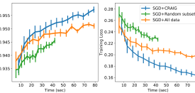
CRAIG achieves considerable speedup. Figure 4 shows training loss and test accuracy for training a 2-layer neural net on MNIST. For this problem, we used a constant learning rate of $10^{-2}$. Here, we apply CRAIG to select a subset of 50% of the data at the beginning of every epoch and train only on the selected subset with the corresponding per-element stepsizes. Interestingly, in addition to achieving a speedup of 2x to 3x for training the network, the subsets selected by CRAIG provide a better generalization performance compared to models trained on the entire dataset.

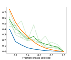
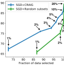
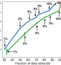
CRAIG is data-efficient for training neural networks. Figure 5 shows test accuracy vs. the fraction of data points selected for training ResNet-20 on CIFAR10. We trained the network for 200 epochs, and used the standard learning rate schedule for training ResNet-20 on CIFAR10. I.e., we start with initial learning rate of 0.1, and exponentially decay the learning rate by a factor of 0.1 at epochs 100 and 150. To prevent weights from diverging when training with subsets of all sizes, we used linear learning rate warm-up for 20 epochs from 0. For optimization we used SGD with a momentum of 0.9.

(a) First

(b) Middle

(c) Last

Figure 6: A subset of images selected by CRAIG from CIFAR10. Subsets are selected at the (a) beginning of training (epoch 1), (b) middle of training (epoch 100), and (c) end of training (epoch 200). We notice that during the training, the semantic redundancies decrease considerably, and coreset images better represent various types of images (that are more difficult to learn) in every class.

Figure 5a shows the test accuracy when at the beginning of every epoch a subset of size 1%, 2%, 3%, 4%, 5%, 10%, or 20% is chosen at random or by CRAIG from the training data. The network is trained only on the selected subset of a given size for that epoch. For every subset size, the x-axis shows the fraction of training data points that are used during the entire training process. Figure 5b shows the test accuracy when a subset of size 1%, 2%, 3%, 4%, 5%, 10%, or 20% is chosen at random or by CRAIG every 5 epochs. The network is trained only on the selected subset for 5 epochs. Generally, larger subsets or more frequent updates lead to more data exposure and hence better performance. However, since in deep networks the gradients may change rapidly after a small number of parameter updates (Defazio & Bottou, 2019), selecting smaller subsets and more frequent updates result in a larger improvement over the random baseline. Note that for a given subset size, backpropagation is done on the same number of data points for CRAIG and random. However, it can be seen that CRAIG can identify the data points that are effective for training the neural network, and hence achieves a superior test accuracy by training on a smaller fraction of the training data.

Insights from CRAIG subsets. Figure 6 shows a subset of images selected by CRAIG for training CIFAR10 at the beginning (6a), middle (6b), and end (6a) of training. Since gradients are more uniformly distributed at initialization, subsets contain semantic redundancies at the beginning of the training (6a). We notice that during the training, semantic redundancies decrease considerably. In particular, as training proceeds coreset images represent groups of images that are more difficult to learn, e.g., contain parts of an object (6b), or have a different foreground/background color than the rest of the images in a class (6c).

6 Conclusion

We developed a method, CRAIG, for selecting a subset (coreset) of data points with their corresponding per-element stepsizes to speed up iterative gradient (IG) methods. In particular, we showed that weighted subsets that minimize the upper-bound on the estimation error of the full gradient, maximize a submodular facility location function. Hence, the subset can be found using a fast greedy algorithm. We proved that IG on subsets $S$ found by CRAIG converges at the same rate as IG on the entire dataset $V$, while providing a $|V|/|S|$ speedup. In our experiments, we showed that various IG methods, including SGD, SAGA, and SVRG runs up to 6x faster on convex and up to 3x on non-convex problems on subsets found by CRAIG while achieving practically the same training loss and test error.

Appendix A Convergence Rate Analysis

We firs proof the following Lemma which is an extension of the [(Chung et al., 1954), Lemma 4].

Lemma 3.

Let $u_{k}\geq 0$ be a sequence of real numbers. Assume there exist $k_{0}$ such that

$$u_{k+1}\leq(1-\frac{c}{k})u_{k}+\frac{e}{k^{p}}+\frac{d}{k^{p+1}},\quad\forall k\geq k_{0},$$

where $e>0,d>0,c>0$ are given real numbers. Then

$$u_{k} \leq(dk^{-1}+e)(c-p+1)^{-1}k^{-p+1}+o(k^{-p+1}) \text{for}~{}c>p-1,p\geq 1$$ (21)

$$u_{k} =O(k^{-c}\log k) \text{for}~{}c=p-1,p>1$$ (22)

$$u_{k} =O(k^{-c}) \text{for}~{}c<p-1,p>1$$ (23)

Proof.

Let $c>p-1$ and $v_{k}=k^{p-1}u_{k}-\frac{d}{k(c-p+1)}-\frac{e}{c-p+1}$. Then, using Taylor approximation $(1+\frac{1}{k})^{p}=(1+\frac{p}{k})+o(\frac{1}{k})$ we can write

$$v_{k+1} =(k+1)^{p-1}u_{k+1}-\frac{d}{(k+1)(c-p+1)}-\frac{e}{c-p+1}$$ (25)

$$\leq k^{p-1}(1+\frac{1}{k})^{p-1}\Big{(}(1-\frac{c}{k})u_{k}+\frac{e}{k^{p}}+\frac{d}{k^{p+1}}\Big{)}-\frac{d}{(k+1)(c-p+1)}-\frac{e}{c-p+1}$$ (26)

$$=k^{p-1}u_{k}\Big{(}1-\frac{c-p+1}{k}+o(\frac{1}{k})\Big{)}+\frac{e}{k}\Big{(}1+\frac{p-1}{k}+o(\frac{1}{k})\Big{)}$$ (27)

$$~{}~{}~{}~{}+\frac{d}{k^{2}}\Big{(}1+\frac{p-1}{k}+o(\frac{1}{k})\Big{)}-\frac{d}{(k+1)(c-p+1)}-\frac{e}{c-p+1}$$ (28)

$$=\Big{(}v_{k}+\frac{d}{k(c-p+1)}+\frac{e}{c-p+1}\Big{)}\Big{(}1-\frac{c-p+1}{k}+o(\frac{1}{k})\Big{)}$$ (29)

$$~{}~{}~{}~{}+\frac{e}{k}\Big{(}1+\frac{p-1}{k}+o(\frac{1}{k})\Big{)}+\frac{d}{k^{2}}\Big{(}1+\frac{p-1}{k}+o(\frac{1}{k})\Big{)}$$ (30)

$$~{}~{}~{}~{}-\frac{d}{(k+1)(c-p+1)}-\frac{e}{c-p+1}$$ (31)

$$=v_{k}\Big{(}1-\frac{c-p+1}{k}+o(\frac{1}{k})\Big{)}+\frac{d/(c-p+1)}{k(k+1)}+\frac{e(p-1)}{k^{2}}+\frac{d(p-1)}{k^{3}}+o(\frac{1}{k^{2}})$$ (32)

Note that for $v_{k}$, we have

$$\sum_{k=0}^{\infty}\Big{(}1-\frac{c-p+1}{k}+o(\frac{1}{k})\Big{)}=\infty$$

and

$$\Big{(}\frac{d/(c-p+1)}{k(k+1)}+\frac{e(p-1)}{k^{2}}+\frac{d(p-1)}{k^{3}}+o(\frac{1}{k^{2}})\Big{)}\Big{(}1-\frac{c-p+1}{k}+o(\frac{1}{k})\Big{)}^{-1}\rightarrow 0.$$

Therefore, $\lim_{k\rightarrow\infty}v_{k}\leq 0$, and we get Eq. 21. For $p=1$, we have $u_{k}\leq\frac{e}{c}$. Hence, $u_{k}$ converges into the region $u\leq\frac{e}{c}$, with ratio $1-\frac{c}{k}$.

Moreover, for $p-1\geq c$ we have

$$v_{k+1} =u_{k+1}(k+1)^{c}\leq\Big{[}(1-\frac{c}{k})u_{k}+\frac{e}{k^{p}}+\frac{d}{k^{p+1}}\Big{]}k^{c}\Big{(}1+\frac{c}{k}+\frac{c^{2}}{2k^{2}}+o(\frac{1}{k^{2}})\Big{)}$$ (33)

$$=\Big{(}1-\frac{c^{2}}{2k^{2}}+o(\frac{1}{k^{2}})\Big{)}v_{k}+\frac{d}{k^{p-c+1}}\Big{(}1+O(\frac{1}{k})\Big{)}+\frac{e}{k^{p-c}}\Big{(}1+\frac{c}{k}+O(\frac{1}{k^{2}})\Big{)}$$ (34)

$$\leq v_{k}+\frac{e^{\prime}}{k^{p-c}}$$ (35)

for sufficiently large $k$. Summing over $k$, we obtain that $v_{k}$ is bounded for $p-1>c$ (since the series $\sum_{k=1}^{\infty}(1/k^{\alpha})$ converges for $\alpha>1$) and $v_{k}=O(\log k)$ for $p=c+1$ (since $\sum_{i=1}^{k}(1/i)=O(\log k)$). ∎

In addition, based on [(Chung et al., 1954), Lemma 5] for $u_{k}\geq 0$, we can write

$$u_{k+1}\leq(1-\frac{c}{k^{s}})u_{k}+\frac{e}{k^{p}}+\frac{d}{k^{t}},\quad\quad 0<s<1,s\leq p<t.$$ (36)

Then, we have

$$u_{k}\leq\frac{e}{c}\frac{1}{k^{p-s}}+o(\frac{1}{k^{p-s}}).$$ (37)

A.1 Convergence Rate for Strongly Convex Functions

Proof of Theorem 1

We now provide the convergence rate for strongly convex functions building on the analysis of (Nedić & Bertsekas, 2001). For non-smooth functions, gradients can be replaced by sub-gradients.

Let $w_{k}=w_{0}^{k}$. For every IG update on subset $S$ we have

$$\|w_{j}^{k}-w_{*}\|^{2} =\|w_{j-1}^{k}-\alpha_{k}\gamma_{j}\nabla f_{j}(w_{j-1}^{k})-w_{*}\|^{2}$$ (38)

$$=\|w_{j-1}^{k}-w_{*}\|^{2}-2\alpha_{k}\gamma_{j}\nabla f_{j}(w_{j-1}^{k})(w_{j-1}^{k}-w_{*})+\alpha_{k}^{2}\|\gamma_{j}\nabla f_{j}(w_{j-1}^{k})\|^{2}$$ (39)

$$\leq\|w_{j-1}^{k}-w_{*}\|^{2}-2\alpha_{k}(f_{j}(w_{j-1}^{k})-f_{i}(w_{*}))+\alpha_{k}^{2}\|\gamma_{i}\nabla f_{j}(w_{j-1}^{k})\|^{2}.$$ (40)

Adding the above inequalities over elements of $S$ we get

$$\|w_{k+1}-w_{*}\|^{2}\leq\|w_{k}-w_{*}\|^{2} -2\alpha_{k}\sum_{j\in S}(f_{i}(w_{j-1}^{k})-f_{j}(w_{*}))+\alpha_{k}^{2}\sum_{j\in S}\|\gamma_{j}\nabla f_{j}(w_{j-1}^{k})\|^{2}$$ (41)

$$=\|w_{k}-w_{*}\|^{2} -2\alpha_{k}\sum_{j\in S}(f_{j}(w_{k})-f_{i}(w_{*}))$$

$$+2\alpha_{k}\sum_{j\in S}(f_{j}(w_{j-1}^{k})-f_{j}(w_{k}))+\alpha_{k}^{2}\sum_{j\in S}\|\gamma_{j}\nabla f_{j}(w_{j-1}^{k})\|^{2}$$ (42)

Using strong convexity we can write

$$\|w_{k+1}-w_{*}\|^{2}\leq\|w_{k}-w_{*}\|^{2} -2\alpha_{k}\big{(}\sum_{j\in S}\gamma_{j}\nabla f_{j}(w_{*})\cdot(w_{k}-w_{*})+\frac{\mu}{2}\|w_{k}-w_{*}\|^{2}\big{)}$$

$$+2\alpha_{k}\sum_{j\in S}(f_{j}(w_{j-1}^{k})-f_{j}(w_{k}))+\alpha_{k}^{2}\sum_{j\in S}\|\gamma_{j}\nabla f_{j}(w_{j-1}^{k})\|^{2}$$ (43)

Using Cauchy–Schwarz inequality, we know

$$|\sum_{j\in S}\gamma_{j}\nabla f_{j}(w_{*})\cdot(w_{k}-w_{*})|\leq\|\sum_{j\in S}\gamma_{j}\nabla f_{j}(w_{*})\|\cdot\|w_{k}-w_{*}\|.$$ (44)

Hence,

$$-\sum_{j\in S}\gamma_{j}\nabla f_{j}(w_{*})\cdot(w_{k}-w_{*})\leq\|\sum_{j\in S}\gamma_{j}\nabla f_{j}(w_{*})\|\cdot\|w_{k}-w_{*}\|.$$ (45)

From reverse triangle inequality, and the facts that $S$ is chosen in a way that $\|\sum_{i\in V}\nabla f_{i}(w_{*})-\sum_{j\in S}\gamma_{j}\nabla f_{j}(w_{*})\|\leq\epsilon$, and that $\sum_{i\in V}\nabla f_{i}(w_{*})=0$ we have $\|\sum_{j\in S}\gamma_{j}\nabla f_{j}(w_{*})\|\leq\|\sum_{i\in V}\nabla f_{i}(w_{*})\|+\epsilon=\epsilon$. Therefore

$$\|\sum_{j\in S}\gamma_{j}\nabla f_{j}(w_{*})\|\cdot\|w_{k}-w_{*}\|\leq\epsilon\cdot\|w_{k}-w_{*}\|$$ (46)

For a continuously differentiable function, the following condition is implied by strong convexity condition

$$\|w_{k}-w_{*}\|\leq\frac{1}{\mu}\|\sum_{j\in S}\gamma_{j}\nabla f_{j}(w_{k})\|.$$ (47)

Assuming gradients have a bounded norm $\max_{\begin{subarray}{c}x\in\mathcal{X},\\ j\in V\end{subarray}}\|\nabla f_{j}(w)\|\leq C$, and the fact that $\sum_{j\in S}\gamma_{j}=n$ we can write

$$\|\sum_{j\in S}\gamma_{j}\nabla f_{j}(w_{k})\|\leq n\cdot C.$$ (48)

Thus for initial distance $\|w_{0}-w_{*}\|=d_{0}$, we have

$$\|w_{k}-w_{*}\|\leq\min(n\cdot C,d_{0})=R$$ (49)

Putting Eq. 45 to Eq. 49 together we get

$$\|w_{k+1}-w_{*}\|^{2}\leq(1-\alpha_{k}\mu) \|w_{k}-w_{*}\|^{2}+2\alpha_{k}\epsilon R/\mu$$

$$+2\alpha_{k}\sum_{j\in S}(f_{j}(w_{j-1,k})-f_{j}(w_{k}))+\alpha_{k}^{2}r\gamma_{\max}^{2}C^{2}.$$ (50)

Now, from convexity of every $f_{j}$ for $j\in S$ we have that

$$f_{j}(w_{k})-f_{j}(w_{j-1}^{k})\leq\|\gamma_{j}\nabla f_{j}(w_{k})\|\cdot\|w_{j-1}^{k}-w_{k}\|.$$ (51)

In addition, incremental updates gives us

$$\|w_{j-1}^{k}-w_{k}\|\leq\alpha_{k}\sum_{i=1}^{j-1}\|\gamma_{i}\nabla f_{i}(w_{i-1}^{k})\|\leq\alpha_{k}(j-1)\gamma_{\max}C.$$ (52)

Therefore, we get

$$2\alpha_{k}\sum_{j\in S}(f_{j}(w_{k})-f_{j}(w_{j-1}^{k})) +\alpha_{k}^{2}r\gamma_{\max}^{2}C^{2}$$

$$\leq 2\alpha_{k}\sum_{i=1}^{r}\gamma_{\max}C\cdot\alpha_{k}(j-1)\gamma_{\max}C+\alpha_{k}^{2}r\gamma_{\max}^{2}C^{2}$$ (53)

$$=\alpha_{k}^{2}r^{2}\gamma_{\max}^{2}C^{2}$$ (54)

Hence,

$$\|w_{k+1}-w_{*}\|^{2}\leq(1-\alpha_{k}\mu)\|w_{k}-w_{*}\|^{2}+2\alpha_{k}\epsilon R/\mu+\alpha_{k}^{2}r^{2}\gamma_{\max}^{2}C^{2}.$$ (55)

where $\gamma_{\text{max}}$ is the size of the largest cluster, and $C$ is the upperbound on the gradients.

For $0<\tau\leq 1$, the theorem follows by applying Lemma 3 to Eq. 55, with $c=\alpha\mu$, $e=2\alpha\epsilon R/\mu$, and $d=\alpha^{2}r^{2}\gamma_{\max}^{2}C^{2}$.

For $\tau=0$, where we have a constant step size $\alpha_{k}=\alpha\leq\frac{1}{\mu}$, we get

$$\|w_{k+1}-w_{*}\|^{2}\leq(1- \alpha\mu)^{k+1}\|w_{0}-w_{*}\|^{2}$$

$$+2\alpha\epsilon R\sum_{j=0}^{k}(1-\alpha\mu)^{j}/\mu+\alpha^{2}r^{2}\gamma_{\max}^{2}C^{2}\sum_{j=0}^{k}(1-\alpha\mu)^{j}$$ (56)

Since $\sum_{j=0}^{k}(1-\alpha\mu)^{j}\leq\frac{1}{\alpha\mu}$, we get

$$\|w_{k+1}-w_{*}\|^{2}\leq(1-\alpha\mu)^{k+1}\|w_{0}-w_{*}\|^{2}+2\alpha\epsilon R/(\alpha\mu^{2})+\alpha^{2}r^{2}\gamma_{\max}^{2}C^{2}/(\alpha\mu),$$ (57)

and therefore,

$$\|w_{k+1}-w_{*}\|^{2}\leq(1-\alpha\mu)^{k+1}\|w_{k}-w_{*}\|^{2}+2\epsilon R/\mu^{2}+\alpha r^{2}\gamma_{\max}^{2}C^{2}/\mu.$$ (58)

A.2 Convergence Rate for Strongly Convex and Smooth Component Functions

Proof of Theorem 2

IG updates for cycle $k$ on subset $S$ can be written as

$$w_{k+1}=w_{k}-\alpha_{k}(\sum_{j\in S}\gamma_{j}\nabla f_{j}(w_{k})-e_{k})$$ (59)

$$e_{k}=\sum_{j\in S}\gamma_{i}(\nabla f_{j}(w_{k})-\nabla f_{j}(w_{j-1}^{k}))$$ (60)

Building on the analysis of (Gürbüzbalaban et al., 2015), for convex and twice continuously differentiable function, we can write

$$\sum_{j\in S}\gamma_{j}\nabla f_{j}(w_{k})-\sum_{j\in S}\gamma_{j}\nabla f_{j}(w_{*})=A_{k}^{r}(w_{k}-w_{*})$$ (61)

where $A_{k}^{r}=\int_{0}^{1}\nabla^{2}f(w_{*}+\tau(w_{k}-w_{*}))d\tau$ is average of the Hessian matrices corresponding to the $r$ (weighted) elements of $S$ on the interval $[w_{k},w_{*}]$.

From Eq. 61 we have

$$\sum_{i\in V}(\nabla f_{i}(w_{k})-\nabla f_{i}(w_{*}))-\sum_{j\in S}\gamma_{j}(\nabla f_{j}(w_{k})-\nabla f_{j}(w_{*}))=A_{k}(w_{k}-w_{*})-A_{k}^{r}(w_{k}-w_{*}),$$ (62)

where $A_{k}$ is average of the Hessian matrices corresponding to all the $n$ component functions on the interval $[w_{k},w_{*}]$. Taking norm of both sides and noting that $\sum_{i\in V}f_{i}(w_{*})=0$ and hence $\|\sum_{j\in S}\gamma_{j}f_{j}(w_{*})\|\leq\epsilon$, we get

$$\|(A_{k}-A_{k}^{r})(w_{k}-w_{*})\|=\|\Big{(}\sum_{i\in V}\nabla f_{i}(w_{k})-\sum_{j\in S}\gamma_{j}\nabla f_{j}(w_{k})\Big{)}+\sum_{j\in S}\gamma_{j}f_{j}(w_{*})\|\leq 2\epsilon,$$ (63)

where $\epsilon$ is the estimation error of the full gradient by the weighted gradients of the elements of the subset $S$, and we used $\|\sum_{i\in V}\nabla f_{i}(w_{k})-\sum_{j\in S}\gamma_{j}\nabla f_{j}(w_{k})\|\leq\epsilon$.

Substituting Eq. 61 into Eq. 59 we obtain

$$w_{k+1}-w_{*}=(I-\alpha_{k}A_{k}^{r})(w_{k}-w_{*})+\alpha_{k}e_{k}$$ (64)

Taking norms of both sides, we get

$$\|w_{k+1}-w_{*}\|\leq\|(I-\alpha_{k}A_{k}^{r})(w_{k}-w_{*}\|)+\alpha_{k}\|e_{k}\|$$ (65)

Now, we have

$$\|(I-\alpha_{k}A_{k}^{r})(w_{k}-w_{*})\| =\|I(w_{k}-w_{*})-\alpha_{k}A_{k}^{r}(w_{k}-w_{*})\|$$ (66)

$$=\|I(w_{k}-w_{*})-\alpha_{k}(A_{k}^{r}-A_{k})(w_{k}-w_{*})-\alpha_{k}A_{k}(w_{k}-w_{*})\|$$ (67)

$$\leq\|(I-\alpha_{k}A_{k})(w_{k}-w_{*})\|+\alpha_{k}\|(A_{k}-A_{k}^{r})(w_{k}-w_{*})\|$$ (68)

$$\leq\|(I-\alpha_{k}A_{k})(w_{k}-w_{*})\|+2\alpha_{k}\epsilon$$ (69)

Substituting into Eq. 65, we obtain

$$\|w_{k+1}-w_{*}\|\leq\|I-\alpha_{k}A_{k}\|\cdot\|w_{k}-w_{*}\|+2\alpha_{k}\epsilon+\alpha_{k}\|e_{k}\|$$ (70)

From strong convexity of $\sum_{i\in V}f_{i}(w)$, and gradient smoothness of each component $f_{i}(w)$ we have

$$\mu I_{n}\preceq\sum_{i\in V}\nabla^{2}f_{i}(w),A_{k}\preceq\beta I_{n},\quad x\in\mathcal{X},$$ (71)

where $\beta=\sum_{i\in V}\beta_{i}$ In addition, from the gradient smoothness of the components we can write

$$\|e_{k}\| \leq\sum_{j\in S}\gamma_{j}\beta_{j}\|w_{k}-w_{j}^{k}\|$$ (72)

$$\leq\sum_{j\in S}\gamma_{j}\beta_{j}\sum_{i=1}^{j-1}\|w_{i-1}^{k}-w_{i}^{k}\|$$ (73)

$$\leq\sum_{j\in S}\gamma_{j}\beta_{j}\alpha_{k}\sum_{i=1}^{j-1}\|\gamma_{i}\nabla f_{i}(w_{i}^{k})\|$$ (74)

$$\leq\alpha_{k}\beta Cr\gamma_{\max}^{2},$$ (75)

where in the last line we used $|S|=r$. Therefore,

$$\|w_{k+1}-w_{*}\| \leq\max(\|1-\alpha_{k}\mu\|,\|1-\alpha_{k}\beta\|)\|w_{k}-w_{*}\|+2\alpha_{k}\epsilon+\alpha_{k}^{2}\beta Cr\gamma_{\max}^{2}$$ (76)

$$\leq(1-\alpha_{k}\mu)\|w_{k}-w_{*}\|+2\alpha_{k}\epsilon+\alpha_{k}^{2}\beta Cr\gamma_{\max}^{2}\quad\text{if}\quad\alpha_{k}\beta\leq 1.$$ (77)

For $0<\tau\leq 1$, the theorem follows by applying Lemma 3 to Eq. 76 with $c=\alpha\mu$, $e=2\alpha\epsilon$, $d=\alpha^{2}\beta Cr\gamma_{\max}^{2}$. For $\tau=0$, where we have a constant step size $\alpha_{k}=\alpha\leq\frac{1}{\beta}$, we get

$$\|w_{k+1}-w_{*}\| \leq(1-\alpha\mu)^{k+1}\|w_{k}-w_{*}\|+2\alpha\epsilon\sum_{i=0}^{k}(1-\alpha\mu)^{i}+\alpha^{2}\sum_{i=0}^{k}(1-\alpha\mu)^{i}\beta Cr\gamma_{\max}^{2}$$ (78)

$$\leq(1-\alpha\mu)^{k+1}\|w_{k}-w_{*}\|+2\epsilon/\mu+\alpha\beta Cr\gamma_{\max}^{2}/\mu,$$ (79)

$$\leq(1-\alpha\mu)^{k+1}\|w_{k}-w_{*}\|+2\epsilon/\mu+Cr\gamma_{\max}^{2}/\mu,$$ (80)

where the inequality in Eq. 79 follows since $\sum_{i=0}^{k}(1-\alpha\mu)^{i}\leq\frac{1}{\alpha\mu}$.

Appendix B Norm of the Difference Between Gradients

B.1 Convex Loss Functions

For ridge regression $f_{i}(w)=\frac{1}{2}(\langle x_{i},w\rangle-y_{i})^{2}+\frac{\lambda}{2}\|w\|^{2}$, we have $\nabla f_{i}(w)=x_{i}(\langle x_{i},w\rangle-y_{i})+\lambda w$. Therefore,

$$\|\nabla f_{i}(w)-\nabla f_{j}(w)\|=(\|x_{i}-x_{j}\|.\|w\|+\|y_{i}-y_{j}\|)\|x_{j}\|$$ (81)

For $\|x_{i}\|\leq 1$, and $|y_{i}-y_{j}|\approx 0$ we get

$$\|\nabla f_{i}(w)-\nabla f_{j}(w)\|\leq\|x_{i}-x_{j}\|O(\|w\|)$$ (82)

For reguralized logistic regression with $y\in\{-1,1\}$, we have $\nabla f_{i}(w)=y_{i}/(1+e^{y_{i}\langle x_{i},w\rangle})$. For $y_{i}=y_{j}$ we get

$$\|\nabla f_{i}(w)-\nabla f_{j}(w)\| = \frac{e^{\|x_{i}-x_{j}\|.\|w\|}-1}{1+e^{-\langle x_{i},x\rangle}}\|x_{j}\|.$$ (83)

For $\|x_{i}\|\leq 1$, using Taylor approximation $e^{x}\leq 1+x$, and noting that $\frac{1}{1+e^{-\langle x_{i},w\rangle}}\leq 1$ we get

$$\|\nabla f_{i}(w)-\nabla f_{j}(w)\|\leq\frac{\|x_{i}-x_{j}\|.\|w\|}{1+e^{-\langle x_{i},w\rangle}}\|x_{j}\|\leq\|x_{i}-x_{j}\|O(\|w\|).$$ (84)

For classification, we require $y_{i}=y_{j}$, hence we can select subsets from each class and then merge the results. On the other hand, in ridge regression we also need $|y_{i}-y_{j}|$ to be small. Similar results can be deduced for other loss functions including square loss, smoothed hinge loss, etc.

Assuming $\|w\|$ is bounded for all $w\in\mathcal{W}$, upper-bounds on the euclidean distances between the gradients can be pre-computed.

B.2 Neural Networks

Formally, consider an $L$-layer perceptron, where $w^{(l)}\in\mathbb{R}^{M_{l}\times M_{l-1}}$ is the weight matrix for layer $l$ with $M_{l}$ hidden units, and $\sigma^{(l)}(.)$ be a Lipschitz continuous activation function. Then, let

$$x_{i}^{(0)} = x_{i},$$ (85)

$$z_{i}^{(l)} = w^{(l)}x_{i}^{(l-1)},$$ (86)

$$x_{i}^{(l)} = \sigma^{(l)}(z_{i}^{(l)}).$$ (87)

With

$$\Sigma^{\prime}_{l}(z_{i}^{(l)}) = \text{diag}\big{(}\sigma^{\prime(l)}(z_{i,1}^{(l)}),\cdots\sigma^{\prime(l)}(z_{i,M_{l}}^{(l)})\big{)},$$ (88)

$$\Delta_{i}^{(l)} = \Sigma^{\prime}_{l}(z_{i}^{(l)})w^{T}_{l+1}\cdots\Sigma^{\prime}_{l}(z_{i}^{(L-1)})w^{T}_{L},$$ (89)

we have

$$\|\nabla f_{i}(w)-\nabla f_{j}(w)\|$$

$$= \|\big{(}\Delta_{i}^{(l)}\Sigma^{\prime}_{L}(z_{i}^{(L)})\nabla f_{i}^{(L)}(w)\big{)}\big{(}x_{i}^{(l-1)}\big{)}^{T}-\big{(}\Delta_{j}^{(l)}\Sigma^{\prime}_{L}(z_{j}^{(L)})\nabla f_{j}^{(L)}(w)\big{)}\big{(}x_{j}^{(l-1)}\big{)}^{T}\|$$ (90)

$$\leq \|\Delta_{i}^{(l)}\|\cdot\|x_{i}^{(l-1)}\|\cdot\|\Sigma^{\prime}_{L}(z_{i}^{(L)})\nabla f_{i}^{(L)}(w)-\Sigma^{\prime}_{L}(z_{j}^{(L)})\nabla f_{j}^{(L)}(w)\|$$

$$+\|\Sigma^{\prime}_{L}(z_{j}^{(L)})\nabla f_{i}^{(L)}(w)\|\cdot\|\Delta_{i}^{(l)}\big{(}x_{i}^{(l-1)}\big{)}^{T}-\Delta_{j}^{(l)}\big{(}x_{j}^{(l-1)}\big{)}^{T}\|$$ (91)

$$\leq \|\Delta_{i}^{(l)}\|\cdot\|x_{i}^{(l-1)}\|\cdot\|\Sigma^{\prime}_{L}(z_{i}^{(L)})\nabla f_{i}^{(L)}(w)-\Sigma^{\prime}_{L}(z_{j}^{(L)})\nabla f_{j}^{(L)}(w)\|$$

$$+\|\Sigma^{\prime}_{L}(z_{j}^{(L)})\nabla f_{i}^{(L)}(w)\|\cdot\big{(}\|\Delta_{i}^{(l)}\|\cdot\|x_{i}^{(l-1)}\|+\|\Delta_{j}^{(l)}\|\cdot\|x_{j}^{(l-1)}\|\big{)}$$ (92)

$$\leq \underbrace{\max_{l,i}\big{(}\|\Delta_{i}^{(l)}\|\cdot\|x_{i}^{(l-1)}\|\big{)}}_{c_{1}}\cdot\|\Sigma^{\prime}_{L}(z_{i}^{(L)})\nabla f_{i}^{(L)}(w)-\Sigma^{\prime}_{L}(z_{j}^{(L)})\nabla f_{j}^{(L)}(w)\|$$

$$+\underbrace{\|\Sigma^{\prime}_{L}(z_{i}^{(L)})\nabla f_{i}^{(L)}(w)\|\cdot\max_{l,i,j}\big{(}\|\Delta_{i}^{(l)}\|\cdot\|x_{i}^{(l-1)}\|+\|\Delta_{j}^{(l)}\|\cdot\|x_{j}^{(l-1)}\|\big{)}}_{c_{2}}$$ (93)

Various weight initialization (Glorot & Bengio, 2010) and activation normalization techniques (Ioffe & Szegedy, 2015; Ba et al., 2016) uniformise the activations across samples. As a result, the variation of the gradient norm is mostly captured by the gradient of the loss function with respect to the pre-activation outputs of the last layer of our neural network (Katharopoulos & Fleuret, 2018). Assuming $\|\Sigma^{\prime}_{L}(z_{i}^{(L)})\nabla f_{i}^{(L)}(w)\|$ is bounded, we get

$$\|\nabla f_{i}(w)-\nabla f_{j}(w)\|\leq c_{1}\|\Sigma^{\prime}_{L}(z_{i}^{(L)})\nabla f_{i}^{(L)}(w)-\Sigma^{\prime}_{L}(z_{j}^{(L)})\nabla f_{j}^{(L)}(w)\|+c_{2},$$ (94)

where $c_{1},c_{2}$ are constants. The above analysis holds for any affine operation followed by a slope-bounded non-linearity $(|\sigma^{\prime}(w)|\leq K)$.

References

- Agarwal et al. (2004) Agarwal, P. K., Har-Peled, S., and Varadarajan, K. R. Approximating extent measures of points. Journal of the ACM (JACM), 51(4):606–635, 2004.
- Allen-Zhu (2017) Allen-Zhu, Z. Katyusha: The first direct acceleration of stochastic gradient methods. The Journal of Machine Learning Research, 18(1):8194–8244, 2017.
- Allen-Zhu et al. (2016) Allen-Zhu, Z., Yuan, Y., and Sridharan, K. Exploiting the structure: Stochastic gradient methods using raw clusters. In Advances in Neural Information Processing Systems, pp. 1642–1650, 2016.
- Asi & Duchi (2019) Asi, H. and Duchi, J. C. The importance of better models in stochastic optimization. arXiv preprint arXiv:1903.08619, 2019.
- Ba et al. (2016) Ba, J. L., Kiros, J. R., and Hinton, G. E. Layer normalization. arXiv preprint arXiv:1607.06450, 2016.
- Bertsekas (1996) Bertsekas, D. P. Incremental least squares methods and the extended kalman filter. SIAM Journal on Optimization, 6(3):807–822, 1996.
- Bertsekas (2015a) Bertsekas, D. P. Convex optimization algorithms. Athena Scientific Belmont, 2015a.
- Bertsekas (2015b) Bertsekas, D. P. Incremental gradient, subgradient, and proximal methods for convex optimization: A survey. arXiv preprint arXiv:1507.01030, 2015b.
- Campbell & Broderick (2018) Campbell, T. and Broderick, T. Bayesian coreset construction via greedy iterative geodesic ascent. In International Conference on Machine Learning, 2018.
- Chung et al. (1954) Chung, K. L. et al. On a stochastic approximation method. The Annals of Mathematical Statistics, 25(3):463–483, 1954.
- Cohen et al. (2017) Cohen, M. B., Musco, C., and Musco, C. Input sparsity time low-rank approximation via ridge leverage score sampling. In Proceedings of the Twenty-Eighth Annual ACM-SIAM Symposium on Discrete Algorithms, pp. 1758–1777. SIAM, 2017.
- Defazio & Bottou (2019) Defazio, A. and Bottou, L. On the ineffectiveness of variance reduced optimization for deep learning. In Advances in Neural Information Processing Systems, pp. 1755–1765, 2019.
- Defazio et al. (2014) Defazio, A., Bach, F., and Lacoste-Julien, S. Saga: A fast incremental gradient method with support for non-strongly convex composite objectives. In Advances in neural information processing systems, pp. 1646–1654, 2014.
- Duchi et al. (2011) Duchi, J., Hazan, E., and Singer, Y. Adaptive subgradient methods for online learning and stochastic optimization. Journal of Machine Learning Research, 12(Jul):2121–2159, 2011.
- Frostig et al. (2015) Frostig, R., Ge, R., Kakade, S., and Sidford, A. Un-regularizing: approximate proximal point and faster stochastic algorithms for empirical risk minimization. In International Conference on Machine Learning, pp. 2540–2548, 2015.
- Glorot & Bengio (2010) Glorot, X. and Bengio, Y. Understanding the difficulty of training deep feedforward neural networks. In Proceedings of the thirteenth international conference on artificial intelligence and statistics, pp. 249–256, 2010.
- Gürbüzbalaban et al. (2015) Gürbüzbalaban, M., Ozdaglar, A., and Parrilo, P. Why random reshuffling beats stochastic gradient descent. arXiv preprint arXiv:1510.08560, 2015.
- Gurbuzbalaban et al. (2017) Gurbuzbalaban, M., Ozdaglar, A., and Parrilo, P. A. On the convergence rate of incremental aggregated gradient algorithms. SIAM Journal on Optimization, 27(2):1035–1048, 2017.
- Har-Peled & Mazumdar (2004) Har-Peled, S. and Mazumdar, S. On coresets for k-means and k-median clustering. In Proceedings of the thirty-sixth annual ACM symposium on Theory of computing, pp. 291–300. ACM, 2004.
- Hofmann et al. (2015) Hofmann, T., Lucchi, A., Lacoste-Julien, S., and McWilliams, B. Variance reduced stochastic gradient descent with neighbors. In Advances in Neural Information Processing Systems, pp. 2305–2313, 2015.
- Ioffe & Szegedy (2015) Ioffe, S. and Szegedy, C. Batch normalization: Accelerating deep network training by reducing internal covariate shift. In International Conference on Machine Learning, pp. 448–456, 2015.
- Johnson & Zhang (2013) Johnson, R. and Zhang, T. Accelerating stochastic gradient descent using predictive variance reduction. In Advances in neural information processing systems, pp. 315–323, 2013.
- Katharopoulos & Fleuret (2018) Katharopoulos, A. and Fleuret, F. Not all samples are created equal: Deep learning with importance sampling. In International Conference on Machine Learning, pp. 2525–2534, 2018.
- Kaufman et al. (1987) Kaufman, L., Rousseeuw, P., and Dodge, Y. Clustering by means of medoids in statistical data analysis based on the, 1987.
- Kingma & Ba (2014) Kingma, D. P. and Ba, J. Adam: A method for stochastic optimization. arXiv preprint arXiv:1412.6980, 2014.
- Li et al. (2013) Li, M., Miller, G. L., and Peng, R. Iterative row sampling. In 2013 IEEE 54th Annual Symposium on Foundations of Computer Science, pp. 127–136. IEEE, 2013.
- Lin & Bilmes (2012) Lin, H. and Bilmes, J. A. Learning mixtures of submodular shells with application to document summarization. arXiv preprint arXiv:1210.4871, 2012.
- Lin et al. (2009) Lin, H., Bilmes, J., and Xie, S. Graph-based submodular selection for extractive summarization. In Proc. IEEE Automatic Speech Recognition and Understanding (ASRU), Merano, Italy, December 2009.
- Lin et al. (2015) Lin, H., Mairal, J., and Harchaoui, Z. A universal catalyst for first-order optimization. In Advances in Neural Information Processing Systems, pp. 3384–3392, 2015.
- Lucic et al. (2017) Lucic, M., Faulkner, M., Krause, A., and Feldman, D. Training gaussian mixture models at scale via coresets. The Journal of Machine Learning Research, 18(1):5885–5909, 2017.
- Mangasariany & Solodovy (1994) Mangasariany, O. and Solodovy, M. Serial and parallel backpropagation convergence via nonmonotone perturbed minimization. 1994.
- Minoux (1978) Minoux, M. Accelerated greedy algorithms for maximizing submodular set functions. In Optimization techniques, pp. 234–243. Springer, 1978.
- Mirzasoleiman et al. (2015a) Mirzasoleiman, B., Badanidiyuru, A., Karbasi, A., Vondrák, J., and Krause, A. Lazier than lazy greedy. In Twenty-Ninth AAAI Conference on Artificial Intelligence, 2015a.
- Mirzasoleiman et al. (2015b) Mirzasoleiman, B., Karbasi, A., Badanidiyuru, A., and Krause, A. Distributed submodular cover: Succinctly summarizing massive data. In Advances in Neural Information Processing Systems, pp. 2881–2889, 2015b.
- Mirzasoleiman et al. (2016) Mirzasoleiman, B., Zadimoghaddam, M., and Karbasi, A. Fast distributed submodular cover: Public-private data summarization. In Advances in Neural Information Processing Systems, pp. 3594–3602, 2016.
- Musco & Musco (2017) Musco, C. and Musco, C. Recursive sampling for the nystrom method. In Advances in Neural Information Processing Systems, pp. 3833–3845, 2017.
- Nedić & Bertsekas (2001) Nedić, A. and Bertsekas, D. Convergence rate of incremental subgradient algorithms. In Stochastic optimization: algorithms and applications, pp. 223–264. Springer, 2001.
- Nemhauser et al. (1978) Nemhauser, G., Wolsey, L., and Fisher, M. An analysis of approximations for maximizing submodular set functions—i. Mathematical Programming, 14(1):265–294, 1978.
- Qian (1999) Qian, N. On the momentum term in gradient descent learning algorithms. Neural networks, 12(1):145–151, 1999.
- Roux et al. (2012) Roux, N. L., Schmidt, M., and Bach, F. R. A stochastic gradient method with an exponential convergence _rate for finite training sets. In Advances in neural information processing systems, pp. 2663–2671, 2012.
- Shalev-Shwartz & Zhang (2013) Shalev-Shwartz, S. and Zhang, T. Stochastic dual coordinate ascent methods for regularized loss minimization. Journal of Machine Learning Research, 14(Feb):567–599, 2013.
- Solodov (1998) Solodov, M. V. Incremental gradient algorithms with stepsizes bounded away from zero. Computational Optimization and Applications, 11(1):23–35, 1998.
- Strubell et al. (2019) Strubell, E., Ganesh, A., and McCallum, A. Energy and policy considerations for deep learning in nlp. arXiv preprint arXiv:1906.02243, 2019.
- Tseng (1998) Tseng, P. An incremental gradient (-projection) method with momentum term and adaptive stepsize rule. SIAM Journal on Optimization, 8(2):506–531, 1998.
- Wei et al. (2015) Wei, K., Iyer, R., and Bilmes, J. Submodularity in data subset selection and active learning. In International Conference on Machine Learning, pp. 1954–1963, 2015.
- Wolsey (1982) Wolsey, L. A. An analysis of the greedy algorithm for the submodular set covering problem. Combinatorica, 2(4):385–393, 1982.
- Xiao & Zhang (2014) Xiao, L. and Zhang, T. A proximal stochastic gradient method with progressive variance reduction. SIAM Journal on Optimization, 24(4):2057–2075, 2014.
- Zeiler (2012) Zeiler, M. D. Adadelta: an adaptive learning rate method. arXiv preprint arXiv:1212.5701, 2012.
- Zhi-Quan & Paul (1994) Zhi-Quan, L. and Paul, T. Analysis of an approximate gradient projection method with applications to the backpropagation algorithm. Optimization Methods and Software, 4(2):85–101, 1994.