Landau theory of bending-to-stretching transition
Abstract
Transition from bending-dominated to stretching-dominated elastic response in semi-flexible fibrous networks plays an important role in the mechanical behavior of cells and tissues. It is induced by changes in network connectivity and relies on construction of new cross-links. We propose a simple continuum model of this transition with macroscopic strain playing the role of order parameter. An unusual feature of this Landau-type theory is that it is based on a single-well potential. We predict that bending-to-stretching transition proceeds through propagation of the localized fronts separating domains with affine and non-affine elastic response.
Typical force transmitting systems in cellular biology can be viewed at the microscale as networks of cross-linked semi-flexible fibers which respond to mechanical loading by both stretching and bending Wilhelm and Frey (2003); Head et al. (2003a); Onck et al. (2005a); Kang et al. (2009); Broedersz and MacKintosh (2014a); Pegoraro et al. (2017). One of the most striking features of such ’materials’ is the loading-induced transition from non-affine, bending-dominated elasticity, to (almost) affine, stretching-dominated elasticity Buxton and Clarke (2007); Mao et al. (2013); Broedersz et al. (2012). This transition is accompanied by the anomalous growth of elastic moduli and is usually linked to the increase of the cross-linker density Feng et al. (2016).
In highly connected dense networks the stretching stiffness dominates because they cannot be deformed without either elongation or shortening of the links; in less dense, under-constrained networks, classical rigidity is lost due to the appearance of floppy modes and softer, bending elasticity becomes responsible for the overall stiffness Head et al. (2003b); Das et al. (2007); Broedersz et al. (2011). The bending-to-stretching (BS) transition was successfully simulated in 2D and 3D athermal microscopic models, and it was found that a continuous crossover between the two regimes takes the form of a highly heterogeneous coexistence between bending (B) and stretching (S) dominated phases Wilhelm and Frey (2003); Head et al. (2003a); Onck et al. (2005a); Buxton and Clarke (2007); Mao et al. (2013); Broedersz et al. (2012).
Despite these successes in microscale modeling, the fundamental understanding of the BS transition at the macroscopic level is still lacking. The development of a coarse-grained model of this phenomenon will facilitate the continuum modeling of cellular scale phenomena Meng and Terentjev (2018); Prost et al. (2015); Bernheim-Groswasser et al. (2018); Burkel et al. (2017); Taloni et al. (2015) and advance the design of the artificial meta-materials with under-connected network architecture Ashby (2006); Broedersz and MacKintosh (2014a); Rocklin et al. (2017).
In this Letter we develop a prototypical Landau-type theory of the strain induced BS transition. We build on the idea that cross-linked networks have the ability to internally rearrange in response to the applied deformation through fiber rotation Onck et al. (2005b); Heussinger and Frey (2006); Wen and Janmey (2013) and that new cross-links can form in this process Gardel et al. (2004); Pegoraro et al. (2017). Our main result is the regime diagram showing how the dominating deformation mode is controlled by the applied strain and the dimensionless ratio of the internal and external length scales.
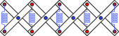
Our approach is deliberately minimalistic. As a prototype of a semi-flexible network, we use a pantographic structure with freely rotating cross-links, as in a collapsible arm of wall mounted mirror van der Giessen (2011). The crucial assumption is that this floppy mechanical system can be stabilized by elastic bonds whose role is to ensure rigidity when they are intact, see Fig. 1.
Suppose that the initial state is chosen in such a way that all vertical springs in Fig. 1 are disengaged and the system is under-constrained Maxwell (1864); Calladine (1978). If such structure is stretched, the geometrical constraints force the system to contract in the vertical direction which can lead to the rebuilding of the bonds. As a result, an under-constrained system transforms into an over-constrained one.
We assume that the floppy structure itself is built of inextensible but flexible beams connected through pivots. It is known that the macroscopic elastic response of the unreinforced pantographic structure shown in Fig. 1 is B-dominated Alibert et al. (2003); more complex examples can be found in the theory of high contrast elastic composites Cherednichenko et al. (2006); Boutin et al. (2013); Camar-Eddine and Seppecher (2003). In the continuum representation of such systems the non-local (higher order) elasticity appears already at the leading order in the homogenization limit which leads to elasticity theories dominated by an internal length scale (as in liquid crystals Chaikin et al. (1995)).
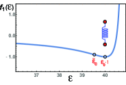
We can then model the discrete structure shown in Fig. 1 as a continuum bar whose classical elastic energy ’softens’ in compression due to breaking of the reinforcing springs. An additive quadratic strain gradient term in the energy density can be used as a proxy for the higher order (non-classical) elasticity of the pantographic frame. With macroscopic strain playing the role of the order parameter Golubović and Lubensky (1989), the ensuing model takes the form of a Ginzburg-Landau (GL) theory Truskinovsky (1996). It is characterized, however, by an unusual vertically flipped Lennard-Jones (Morse) type potential, see Fig. 2.
We use this continuum model to show that the quasi-statically driven BS transition proceeds through nucleation and propagation of the fronts separating domains with affine and non-affine elastic response. At such fronts, the connectivity of the network changes and they can be interpreted as the (degenerate) domain walls. In contrast to the mixed BS states, the pure B and S states are homogeneous. We show, however, that in the B states the affinity, imposed by the weak gradient elasticity, is not robust.
To mimic realistic systems we also consider the GL model with a constraining elastic background Das and MacKintosh (2011), either imitating surrounding matrix Zhang et al. (2013a) or representing non-mechanical long-range signaling Zhang et al. (2013b); Rens et al. (2018); van Doorn et al. (2017). The resultant competing interactions generate in the mixed BS regime stable periodic patterns reminiscent of what is usually observed in other reinforced fragile systems Xia and Hutchinson (2000); Fantilli et al. (2009); Novak and Truskinovsky (2017).
We write the dimensionless energy of our 1D system in the form where the energy density has an additive structure Here is the longitudinal strain, is the displacement of point and prime denotes the derivative. The term is a single well potential describing a breakable springs; in computations we use a particular expression where is the reference strain (see Fig. 2), however, our general results are independent of this choice. With such potential, the system’s rigidity is sound for sufficiently large stretching while compression makes the response progressively softer. The second term in the expression for describes the bending energy of the pantographic structure and, following Alibert et al. (2003), we assume that where is an internal length scale. The resulting model has the classical GL structure.
We further assume that the system is loaded in the “hard” loading device which means that the control parameter is the applied strain , so that, for instance, . We also suppose that the boundaries of our ’bar’ are ’moment free’ in the sense that Under these conditions we need to minimize the elastic energy functional . The affine configuration is always an equilibrium state, however, it is not always stable. To find the instability threshold we study a linearized problem involving the displacement perturbation . The problem reduces to finding nontrivial solutions of the linear equation
| (1) |
where and the boundary conditions are: The non-affine modes appear at solving the characteristic equation
| (2) |
The analysis of (2) for our choice of the function shows that the affine configuration is locally stable for sufficiently small and for sufficiently large . Both direct (affine-non-affine) and return (non-affine-affine) instabilities are of long wave nature with the same critical wavelength Note that , where is the spinodal limit satisfying , so the non-affine configurations are located inside the concavity domain of the potential .
We associate stable affine states at with S-dominated regimes and at – with B-dominated regimes. In S regimes the affine character of the deformation is secured by the presence of classical elasticity. The latter becomes destabilizing in the B regimes where the affinity is safeguarded by the (non-classical) gradient elasticity.
To account for nonlocal interactions in the realistic biological systems we now embed our floppy frame into an elastic environment. To this end we introduce linear coupling of the GL system with a pre-stretched background Truskinovsky and Zanzotto (1996); Ren and Truskinovsky (2000). The anti-ferromagnetic effect of the elastic environment will then compete with the ferromagnetic effect of the bending term in the energy and the resulting microstructures can be more complex.
We need to consider the dimensionless energy Vainchtein et al. (1999)
| (3) |
where is the external length scale characterizing the relative size of the embedding matrix. Since the order parameter is , the account of environmental elasticity brings implicit nonlocality into the conventional structure of a GL theory Ren and Truskinovsky (2000).
The linear instability condition for the affine state in the model (3) takes the form
| (4) |
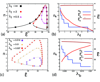
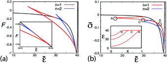
One can show that the redressed upper and lower critical strains correspond again to the same critical wavelength, however, can now take arbitrary large values. In Fig. 3 we illustrate the resulting dependence of the critical parameters on dimensionless lengths and .
Note that the re-entry structure of the bifurcation, found in the local GL system, persists at moderate nonlocality, however, the non-affinity domain disappears when the internal () and external () length scales become comparable. The parametric dependence of the critical wavelength takes the form of a staircase which suggests that particular patterns are robust.
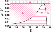
The obtained results can be summarized in the form of a regime diagram. For infinite system, where one can disregard the discreteness of the problem, we can write an approximate equation for the critical strain in the form
| (5) |
The solution of (5) can be used as a rough description of the boundary delineating the pure B and S regimes from the mixed BS regime. In the ensuing diagram (see Fig. 4) the applied strain plays the role analogous to the cross-linker density, while the ratio characterizes the stabilizing strength of the elastic environment. In the matrix-dominated (super-critical) regime M the deformation is always affine.
To explore the structure of the nonlinear energy minimizing configurations we need to solve the equation
| (6) |
In the limiting case the nonlocality is absent and the energy minimizers have the basic GL structure with a single domain boundary separating the phase where the springs are broken, and the elasticity is of B type, from the phase where they are intact, and the dominating elasticity is of the S type. Other equilibrium branches, describing more complex mixtures of such phases, have higher energy, see Fig. 5 where we show the equilibrium energy and the macro stress .
The ensuing two phase configurations, however, are far from being conventional. Consider, for instance, a stretching loading protocol originating in the homogeneous B phase, and assume that the system always remains in the ground state. The nucleation of the S phase takes place discontinuously with the formation of the configuration A ( see Fig. 5b) exhibiting a localized front separating the affine S phase and the non-affine B phase. As the applied strain increases, the homogeneous S phase proliferates with successive springs reconnecting. During this process the shrinking B phase maintains a particular pattern of non-affinity (see configurations C and D in Fig. 5b). The S phase finally takes over through a discontinuous event of the final annihilation of the B phase. From the perspective of nonlinear stability theory we observe here a typical ’isola’ bifurcation of re-entry type Dellwo et al. (1982).
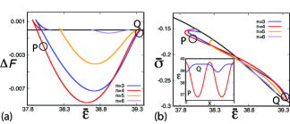
Consider now the case when the elastic environment is present (). The bending energy term then favors coarsening while the nonlocal term drives the refinement of the microstructure and the ensuing competition leads to the formation of BS mixtures with more complex geometry. In Fig. 6 we show the typical configuration of the low energy branches. Note that the topological structure of the micro-configuration changes along the global minimum path: we observe a switch from a configuration with four to a configuration with three BS interfaces.
As the total strain increases beyond the point P, the homogeneous B phase loses stability which leads to collective nucleation of the periodically placed islands of the affine S phase while the remaining B phase becomes non-affine. With further increase of , the islands of S phase grow in size, see point Q, and eventually B phase completely disappears.
We now return to the observation that in our simple tests the deformation in the pure S and B phases was affine; the non-affine response was observed only in the BS (mixed) phase. We recall that in experiments involving fibrous disordered networks, the non-affinity of the deformation was found in the whole range of the B-dominated elastic response Broedersz and MacKintosh (2014b). These observations can be explained by the fragility of affine response in B phase while it is robust in S phase.
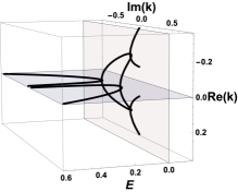
Indeed, consider again the linear modes superimposed on a homogeneous solution of (6). The normalized wave numbers must satisfy the characteristic equation where for convenience we now introduced directly the tangential elastic modulus . The complex solutions of this equation are shown in Fig. 7.
Note that in S phase the roots are purely imaginary. They describe exponential decay of the local mechanical perturbations and are characteristic for systems with affine response. Instead, in B phase the characteristic wave numbers are real and the perturbations spread over the whole system signaling non-affine response. In the crossover range, where and the scales and are comparable (see (5) for the more precise characterization), the wave numbers are complex and the response is mixed.
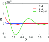
To further support these observations we again linearize (6) but now impose a localized perturbations :
| (7) |
The response to such force distribution, when it is applied near one of the ends of the bar, is illustrated in Fig. 8. We see an almost unperturbed affine response in the S phase, a limited penetration of the perturbation in the BS phase and a markedly non-affine global response in the B phase.
To show that these observations are not conditioned to the case with elastic environment, consider a linearized problem for a bar with which is clamped on one side and loaded on the other side by a force . Suppose that the bending rigidity is sufficiently small, so that in S phase we can neglect bending and relax the clamping boundary condition. Under these assumptions the problem reduces to solving the equation with the boundary conditions . The resulting response is affine: . Now consider B phase, where the stiffness can be neglected and the equilibrium equation is , while the boundary conditions are . The solution of this boundary value problem is globally inhomogeneous: .
To conclude, we presented a prototypical continuum model of the BS transition. The proposed theory describes the peculiar nucleation and propagation of S-dominated domains inside a bar with B-dominated elasticity. It also explains the fundamental non-affinity of the B-phase and rationalizes the observed heterogeneity of the mixed BS phase. To make the model more biologically relevant it will be necessary to account for the fact that in cellular systems the BS transition can be also driven actively Bertrand et al. (2012); Alvarado et al. (2013).
We thank P. Recho and P. Ciarletta for helpful discussions. The work was supported by the grants ANR-18-CE42-0017 (OUS) and ANR-10-IDEX-0001-02 PSL (LT).
References
- Wilhelm and Frey (2003) J. Wilhelm and E. Frey, Phys. Rev. Lett. 91, 108103 (2003).
- Head et al. (2003a) D. A. Head, A. J. Levine, and F. C. MacKintosh, Phys. Rev. E 68, 061907 (2003a).
- Onck et al. (2005a) P. R. Onck, T. Koeman, T. Van Dillen, and E. Van der Giessen, Phys. Rev. Lett. 95(17) (2005a).
- Kang et al. (2009) H. Kang, Q. Wen, P. A. Janmey, J. X. Tang, E. Conti, and F. C. MacKintosh, J. Phys. Chem. B 113, 3799 (2009).
- Broedersz and MacKintosh (2014a) C. P. Broedersz and F. C. MacKintosh, Rev. Mod. Phys. 86, 995 (2014a).
- Pegoraro et al. (2017) A. F. Pegoraro, P. Janmey, and D. A. Weitz, Cold Spring Harb. Perspect. Biol. 9 (2017).
- Buxton and Clarke (2007) G. A. Buxton and N. Clarke, Phys. Rev. Lett. 98(23) (2007).
- Mao et al. (2013) X. Mao, O. Stenull, and T. C. Lubensky, Phys. Rev. E 87, 042601 (2013).
- Broedersz et al. (2012) C. P. Broedersz, M. Sheinman, and F. C. MacKintosh, Phys. Rev. Lett. 108, 078102 (2012).
- Feng et al. (2016) J. Feng, H. Levine, X. Mao, and L. M. Sander, Soft Matter 12, 1419 (2016).
- Head et al. (2003b) D. A. Head, A. J. Levine, and F. C. MacKintosh, Phys. Rev. Lett. 91, 108102 (2003b).
- Das et al. (2007) M. Das, F. C. MacKintosh, and A. J. Levine, Phys. Rev. Lett. 99, 038101 (2007).
- Broedersz et al. (2011) C. P. Broedersz, X. Mao, T. C. Lubensky, and F. C. MacKintosh, Nat. Phys. 7, 983 (2011).
- Meng and Terentjev (2018) F. Meng and E. M. Terentjev, Macromolecules 51, 4660 (2018).
- Prost et al. (2015) J. Prost, F. Jülicher, and J.-F. Joanny, Nat. Phys. 11, 111 (2015).
- Bernheim-Groswasser et al. (2018) A. Bernheim-Groswasser, N. S. Gov, S. A. Safran, and S. Tzlil, Adv. Mater. 30, 1707028 (2018).
- Burkel et al. (2017) B. Burkel, A. Lesman, P. Rosakis, D. A. Tirrell, G. Ravichandran, and J. Notbohm, in Mechanics of Biological Systems and Materials, Volume 6 (Springer International Publishing, 2017) pp. 135–141.
- Taloni et al. (2015) A. Taloni, E. Kardash, O. U. Salman, L. Truskinovsky, S. Zapperi, and C. A. M. La Porta, Phys. Rev. Lett. 114, 208101 (2015).
- Ashby (2006) M. F. Ashby, Philos. Trans. A Math. Phys. Eng. Sci. 364, 15 (2006).
- Rocklin et al. (2017) D. Z. Rocklin, S. Zhou, K. Sun, and X. Mao, Nat. Commun. 8, 14201 (2017).
- Gardel et al. (2004) M. L. Gardel, J. H. Shin, F. C. MacKintosh, L. Mahadevan, P. Matsudaira, and D. A. Weitz, Science 304, 1301 (2004).
- Onck et al. (2005b) P. R. Onck, T. Koeman, T. van Dillen, and E. van der Giessen, Phys. Rev. Lett. 95, 178102 (2005b).
- Heussinger and Frey (2006) C. Heussinger and E. Frey, Phys. Rev. Lett. 97, 105501 (2006).
- Wen and Janmey (2013) Q. Wen and P. A. Janmey, Exp. Cell Res. 319, 2481 (2013).
- van der Giessen (2011) E. van der Giessen, Nat Phys 7, 923 (2011).
- Maxwell (1864) J. C. Maxwell, The London, Edinburgh, and Dublin Philosophical Magazine and Journal of Science 27, 294 (1864).
- Calladine (1978) C. R. Calladine, Int. J. Solids Struct. 14, 161 (1978).
- Alibert et al. (2003) J.-J. Alibert, P. Seppecher, and F. Dell’Isola, Mathematics and Mechanics of Solids 8, 51 (2003).
- Cherednichenko et al. (2006) K. D. Cherednichenko, V. P. Smyshlyaev, and V. V. Zhikov, Proceedings of the Royal Society of Edinburgh: Section A Mathematics 136 (2006).
- Boutin et al. (2013) C. Boutin, J. Soubestre, M. S. Dietz, and C. Taylor, European Journal of Mechanics-A/Solids 42 (2013).
- Camar-Eddine and Seppecher (2003) M. Camar-Eddine and P. Seppecher, Archive for rational mechanics and analysis 170 (2003).
- Chaikin et al. (1995) P. M. Chaikin, T. C. Lubensky, and T. A. Witten, Principles of condensed matter physics, Vol. 1 (Cambridge university press Cambridge, 1995).
- Golubović and Lubensky (1989) L. Golubović and T. C. Lubensky, Phys. Rev. Lett. 63(10) (1989).
- Truskinovsky (1996) L. Truskinovsky, in Contemporary research in the mechanics and mathematics of materials CIMNE, Barcelona, 322-332 (1996).
- Das and MacKintosh (2011) M. Das and F. C. MacKintosh, Phys. Rev. E 84, 061906 (2011).
- Zhang et al. (2013a) L. Zhang, S. P. Lake, V. H. Barocas, M. S. Shephard, and R. C. Picu, Soft Matter 9, 6398 (2013a).
- Zhang et al. (2013b) L. Zhang, S. P. Lake, V. H. Barocas, M. S. Shephard, and R. C. Picu, Soft Matter 9, 6398 (2013b).
- Rens et al. (2018) R. Rens, C. Villarroel, G. Düring, and E. Lerner, Phys. Rev. E 98, 062411 (2018).
- van Doorn et al. (2017) J. M. van Doorn, L. Lageschaar, J. Sprakel, and J. van der Gucht, Phys Rev E 95, 042503 (2017).
- Xia and Hutchinson (2000) Z. Xia and J. W. Hutchinson, Journal of the Mechanics and Physics of Solids 48, 1107 (2000).
- Fantilli et al. (2009) A. P. Fantilli, H. Mihashi, and P. Vallini, Cement and Concrete Research 39, 1217 (2009).
- Ren and Truskinovsky (2000) X. Ren and L. Truskinovsky, Journal of elasticity 59, 319 (2000).
- Truskinovsky and Zanzotto (1996) L. Truskinovsky and G. Zanzotto, J. Mech. Phys. Solids 44, 1371 (1996).
- Novak and Truskinovsky (2017) I. Novak and L. Truskinovsky, Philos. Trans. A Math. Phys. Eng. Sci. 375 (2017).
- Vainchtein et al. (1999) A. Vainchtein, T. J. Healey, and P. Rosakis, Computer Methods in Applied Mechanics and Engineering 170, 407 (1999).
- Dellwo et al. (1982) D. Dellwo, H. B. Keller, B. J. Matkowsky, and E. L. Reiss, SIAM Journal on Applied Mathematics 42 (1982).
- Broedersz and MacKintosh (2014b) C. P. Broedersz and F. C. MacKintosh, Rev. Mod. Phys. 86, 995 (2014b).
- Bertrand et al. (2012) O. J. N. Bertrand, D. K. Fygenson, and O. A. Saleh, Proceedings of the National Academy of Sciences 109, 17342 (2012).
- Alvarado et al. (2013) J. Alvarado, M. Sheinman, A. Sharma, F. C. MacKintosh, and G. H. Koenderink, Nat Phys 9, 591 (2013).