Fréchet random forests for metric space valued regression with non euclidean predictors

Abstract

Random forests are a statistical learning method widely used in many areas of scientific research because of its ability to learn complex relationships between input and output variables and also their capacity to handle high-dimensional data. However, current random forest approaches are not flexible enough to handle heterogeneous data such as curves, images and shapes. In this paper, we introduce Fréchet trees and Fréchet random forests, which allow to handle data for which input and output variables take values in general metric spaces (which can be unordered). To this end, a new way of splitting the nodes of trees is introduced and the prediction procedures of trees and forests are generalized. Then, random forests out-of-bag error and variable importance score are naturally adapted. A consistency theorem for Fréchet regressogram predictor using data-driven partitions is given and applied to Fréchet purely uniformly random trees. The method is studied through several simulation scenarios on heterogeneous data combining longitudinal, image and scalar data. Finally, two real datasets from HIV vaccine trials are analyzed with the proposed method.

Keywords Random forests  $\cdot$ Nonparametric regression  $\cdot$ Metric spaces regression  $\cdot$ Longitudinal data  $\cdot$ heterogeneous data

1 Introduction

Random Forests [Breiman, 2001] are one of the state-of-the-art machine learning methods. It owes its success to very good predictive performance coupled with very few parameters to tune. Moreover, as a tree-based method, it is able to handle regression and classification (2-class or multi-class) problems in a consistent manner and deals with quantitative or qualitative input variables. Finally, its non-parametric nature allows to proceed high-dimensional data where the number of input variables is very large in regards of statistical units.

The general principle of a tree predictor is to recursively partition the input space. Starting from the root node which contains all learning observations, it repeatedly splits each node into two or more child nodes until a stopping rule is reached. Let us focus, for the sake of clarity, on the case where all input variables are quantitative. For most of tree predictors, splits are binary and consist in an input variable $X^{j}$ and a threshold $s$, leading to two child nodes containing observations that verify $\{X^{j}\leq s\}$ and $\{X^{j}>s\}$ respectively [Breiman et al., 1984]. The splitting variable as well as the threshold are most of the time sought to minimize an heterogeneity criterion on child nodes. The main idea is to partition the input space into more and more homogeneous regions in terms of the output variable.

One limitation of the previously described splitting strategy is that all input variables must live in an ordered space (the method must decide if an observation of the splitting variable is less or larger than the threshold). Yet, with complex data structures, inputs can belong to unordered spaces. As an illustrative example, the real datasets to be analyzed in this paper are from HIV vaccine trials made of input and output variables which are discretely sampled curves representing repeated measurements over time. This example typically corresponds to observations collected in longitudinal studies. In such settings, a main objective is to predict for a given individual the output trajectory given the knowledge of inputs trajectories. If this objective is reached at the trajectory level, then the notion of order between explanatory variables is lost. However, ignoring the fact that measurements are repeated observations over time generally leads to an important loss of information for prediction. Thus, one way of analyzing this kind of data is to generalize the notion of split in unordered metric spaces. Recently, random forests have been adapted to the general metric space framework but in the special case where neither the representation of the data nor the distances between data points are available [Haghiri et al., 2018]. In the present work, we take into account the distances between any items of the space.

Hence, we consider the framework of a learning sample $\mathcal{L}_{n}=\{(X_{1},Y_{1}),\ldots,(X_{n},X_{n})\}$ made of i.i.d. observations of a pair of random variable $(X,Y)\in\mathcal{X}\times\mathcal{Y}$, where $\mathcal{X}$ is a product of $p$ metric spaces (which can be unordered) $(\mathcal{X}_{1},d_{1})\times\cdots\times(\mathcal{X}_{p},d_{p})$, and where $\mathcal{Y}$ is also a metric space with distance $d_{\mathcal{Y}}$. The core idea of this work is to generalize the notion of split that only uses the distance of each metric space. Furthermore, as the notion of mean in the output space $\mathcal{Y}$ is also needed to allocate predictions to terminal nodes of a tree, the Fréchet mean that generalizes the mean in general metric spaces [Fréchet, 1906] is used. This justifies the names Fréchet trees and Fréchet random forests hereafter. Once the notion of split is defined, the building of a maximal tree and the pruning of that tree to obtain an optimal tree are extended. Finally, with this generalization of CART trees, Fréchet random forests are derived in a rather standard way: a forest predictor is an aggregation of a collection of randomized trees. In our framework, the aggregation step therefore consists in taking the Fréchet mean of individual tree predictions.

The use of the Fréchet mean has now become a standard tool for statistical inference from manifold-valued data. For example, it is the key notion allowing to perform PCA for non-Euclidean data such as functional data on Riemanian manifolds (see e.g. [Dai and Muller, 2018], [Fletcher et al., 2004], [Sommer et al., 2010]) or histograms [Cazelles et al., 2018], and to analyze ensemble of complex objects with their shape, such as ECG curves [Bigot, 2013] or phylogenetic trees [Nye et al., 2017]. New innovative regression methods have also emerged for the framework of a metric space valued output variable with Euclidean predictors [Petersen and Müller, 2019]. The methods proposed in this paper allow to perform nonparametric regression between predictors taking their values in different metric spaces and a metric space valued output.

In this paper, we first present the Fréchet tree predictor in Section 2 before introducing Fréchet random forests in Section 3. We introduce an extremely randomized version of the Fréchet random forests method in Section 3.3. Section 4 is dedicated to the analysis of the consistency of Fréchet regressogram estimators using data-driven partitions with output lying in metric space. We report numerical experiments using simulated longitudinal data to compare our approach with competitive methods, then we analyze two scenarios of heterogeneous data simulations involving curves, images and scalars in Section 5. An application of Fréchet random forests for statistical inference from longitudinal data is presented in Section 6. Finally, we discuss in Section 7 potential extensions of this work. All the numerical experiments of this paper are reproducible from our R package FrechForest.

2 Fréchet Trees

2.1 Fréchet means and Fréchet variance

The notions of mean and variance are central to the construction of regression trees [Breiman et al., 1984]. We introduce in this section the notions of Fréchet empirical mean and Fréchet empirical variance [Fréchet, 1948], which are the natural generalization of mean and variance in metric spaces. Let $(z_{1},\ldots,z_{n})$ a sample from a metric space $\left(\mathcal{Z},d\right)$, the empirical Fréchet function is given by

$$\begin{array}[]{ccccc}\mathcal{F}_{n}&:&\mathcal{Z}&\longmapsto&\mathbb{R}^{+}\\ &&z&\longmapsto&\frac{1}{n}\overset{n}{\underset{i=1}{\sum}}d^{2}(z,z_{i})\\ \end{array}$$

the function $\mathcal{F}_{n}(z)$ measures the average squared distance between $z\in\mathcal{Z}$ and $z_{1},\ldots,z_{n}$. We define the empirical Fréchet means $\overline{z}_{n}$ of the sample $(z_{1},\ldots,z_{n})$ as any minimizer of the empirical Fréchet function, i.e.

$$\overline{z}_{n}\in\underset{z\in\mathcal{Z}}{\operatorname*{arg\,min}}\ \mathcal{F}_{n}(z)$$

Note that the Fréchet mean can be non unique. The empirical Fréchet variance $\mathcal{V}_{n}$ of the sample $(z_{1},\ldots,z_{n})$ is then given by

$$\mathcal{V}_{n}=\mathcal{F}_{n}(\overline{z}_{n})=\frac{1}{n}\sum_{i=1}^{n}d^{2}(z_{i},\overline{z}_{n})$$

Note that even if the empirical Fréchet mean may not be a unique element of the metric space, the Fréchet variance is unique. Throughout the paper, Fréchet’s mean and Fréchet variance will always refer to Fréchet empirical mean and Fréchet’s empirical variance. For the sake of simplicity, we assume in the rest of the paper that the Fréchet mean is unique.

2.2 Splitting rule

One key ingredient in the building of a decision tree is the way its nodes are split [Breiman et al., 1984]. Splitting a node $t$ of a tree according to some variable $X^{(j)}$ amounts to find a way of grouping observations of this node into two subsets constituting the child nodes. This grouping is usually performed to maximize the differences between the two resulting child nodes according to the output variable. However, if variable $X^{(j)}$ is strongly related to the output variable $Y$, then it is expected that for two observations with "close" $X^{(j)}$ values in $(\mathcal{X}_{j},d_{j})$, associated outputs will be "close" in $(\mathcal{Y},d_{\mathcal{Y}})$. From this idea, we introduce a way of splitting nodes in general metric spaces.  Let $\left(\mathcal{Z},d\right)$ be a metric space, a split is any couple of distinct elements $\left(c_{1},c_{2}\right)$ of $\mathcal{Z}$. We define the partition $\mathcal{P}=\left\{P_{1},P_{2}\right\}$ associated with elements $\left(c_{1},c_{2}\right)$ by $P_{1}=\left\{z\in\mathcal{Z},d\left(z,c_{1}\right)\leq d\left(z,c_{2}\right)\right\}$ and $P_{2}=\left\{z\in\mathcal{Z},d\left(z,c_{2}\right)<d\left(z,c_{1}\right)\right\}$.
Let $A$ be a subset of the input space $\mathcal{X}$ and for any $j=1,\ldots,p$, let $A_{j}=\{x^{(j)},x=\left(x^{(1)},\ldots,x^{(p)}\right)\in A\}$ denotes the set of the $j$-th coordinates of the components of A. Let $\left(c_{j,l},c_{j,r}\right)$ be a split on $(A_{j},d_{j})$, denote $A_{j,r}$ and $A_{j,l}$ the right and left child nodes (i.e. the associated partition) obtained from the split $\left(c_{j,l},c_{j,r}\right)$.
The quality of the split $\left(c_{j,l},c_{j,r}\right)$ is then defined by the following measure of Fréchet variance decrease:

$$H_{n,j}(A,c_{j,l},c_{j,r})=\mathcal{V}_{n}(A)-\frac{N_{n}\left(A_{j,r}\right)}{N_{n}\left(A\right)}\mathcal{V}_{n}(A_{j,r})-\frac{N_{n}\left(A_{j,l}\right)}{N_{n}\left(A\right)}\mathcal{V}_{n}(A_{j,l})$$ (1)

where $N_{n}(A)$ is the number of observations of the learning set $\mathcal{L}_{n}$ belonging to $A$ and $\mathcal{V}_{n}(A),\ \mathcal{V}_{n}(A_{j,l})$ and $\mathcal{V}_{n}(A_{j,r})$ are the empirical Fréchet variances of outputs in $A$, $A_{j,r}$ and $A_{j,l}$ i.e.

$$\mathcal{V}_{n}(A)=\frac{1}{N_{n}(A)}\sum_{i:X_{i}\in A}d_{\mathcal{Y}}^{2}(Y_{i},\overline{Y}_{A})\qquad\mbox{(resp. for $A_{j,l}$ and $A_{j,r}$).}$$

$\overline{Y}_{A}$, $\overline{Y}_{A_{j,l}}$ and $\overline{Y}_{A_{j,r}}$ are the Fréchet means of outputs associated to observations belonging to nodes $A$, $A_{j,l}$ and $A_{j,r}$ i.e.

$$\overline{Y}_{A}=\operatorname*{arg\,min}_{y\in\mathcal{Y}}\sum_{i:X_{i}\in A}d_{\mathcal{Y}}^{2}(y,Y_{i})\qquad\mbox{(resp. for $\overline{Y}_{A_{j,l}}$ and $\overline{Y}_{A_{j,r}}$).}$$

It is worth noting that the decrease in Fréchet variance for each possible split is compared with the output space metric, which makes it possible to compare splits made on input variables from different metric spaces. At last, the split variable $j_{n}^{*}$, chosen for splitting the node is the one that maximizes $H_{n,j}$, that is

$$j_{n}^{*}=\operatorname*{arg\,max}_{j\in\{1,\ldots,p\}}H_{n,j}\enspace.$$ (2)

It is easy to show that $H_{n,j_{n}^{*}}\geq 0$ for all $n$, thanks to the use of the Fréchet mean, which means that each split leads to a decrease of Fréchet variance.

To determine the successive splits $(c_{j,l},c_{j,r})$, the user defines, in a preliminary step, a split function i.e. a way to find the two representatives $(c_{j,l},c_{j,r})$. More precisely, a split function is an application which associates a couple $\left(c_{1},c_{2}\right)\in\mathcal{Z}$ to any sample $\{h_{1},\ldots,h_{n}\}$ from a general metric space $\left(\mathcal{Z},d\right)$. For example, the $2$-means algorithm ($k$-means with $k=2$) can be used to determine the representatives. Note that for each metric space $\left(\mathcal{X}_{j},d_{j}\right)$ we can use a different split function.

2.3 Tree building

Starting from the root node (associated with the whole input space $\mathcal{X}$), nodes are recursively split in order to give a partition of the input space $\mathcal{X}$. A node $t$ of the tree is not split if it is pure, that is if the Fréchet variance of this node is null. As a first step in the building process, the tree is developed until all nodes are pure, leading to the so-called maximal tree. Then, the pruning algorithm of CART [Breiman et al., 1984] is applied, with the use of the Fréchet variance instead of the standard empirical variance. At the end of this step, a sequence of nested sub-trees of the maximal tree is obtained. Next, the sub-tree associated to the lowest prediction error (estimated by cross-validation) is selected as the final tree predictor. The way a Fréchet tree predicts new inputs is detailed in the next section.

2.4 Prediction

Let $T_{n}$ be a Fréchet tree, we note $\widetilde{T}_{n}$ the set of leaves (i.e., terminal nodes) of $T_{n}$. For each leaf $t\in\widetilde{T}_{n}$, the Fréchet mean of the outputs of observations belonging to $t$ is associated to $t$. Then the prediction of the output variable associated with any $x\in\mathcal{X}$ is given by $\widehat{y}=T_{n}(x)=\sum_{t\in\widetilde{T}_{n}}\overline{Y}_{t}\mathbb{1}_{x\in t}$, where $\mathbb{1}_{S}$ denotes the indicator function of a set $S$ and $\overline{Y}_{t}$ is the Fréchet mean of outputs in $t$

$$\overline{Y}_{t}=\underset{y\in\mathcal{Y}}{\operatorname*{arg\,min}}\sum_{i:X_{i}\in t}d_{\mathcal{Y}}^{2}\left(y,Y_{i}\right)$$

In order to determine to which leaf belongs an observation $x$, it is dropped down the tree as follows. Starting from the root node, the associated split variable $X^{(j_{1})}$ is considered, together with its two child nodes $A_{j_{1},l}$ and $A_{j_{1},r}$, as well as the corresponding representatives $c_{j_{1},l}$ and $c_{j_{1},l}$. To decide in which child node $x$ must fall, its $d_{j_{1}}$-distance with $c_{j_{1},l}$ and $c_{j_{1},l}$ must be computed and $x$ goes to $A_{j_{1},l}$ if $d_{j_{1}}(x^{(j_{1})},c_{j_{1},l})<d_{j_{1}}(x^{(j_{1})},c_{j_{1},r})$ and to $A_{j_{1},r}$ otherwise. This process is then repeated until $x$ falls into a leaf. The error made by $T_{n}$ on $x$ is defined as:

$$\mathrm{err}(T_{n}(x))=d^{2}_{\mathcal{Y}}(T_{n}(x),y)\enspace.$$

3 Fréchet random forests

3.1 An aggregation of Fréchet trees

A Fréchet random forest is derived as standard random forests [Breiman, 2001]: it consists in an aggregation of a collection of randomized Fréchet trees. Here, the same random perturbations as standard random forests [Breiman, 2001] are used. Let $l\in\{1,\ldots,q\}$ and consider the $l$-th tree. First, it is built on a bootstrap sample of the learning sample $\mathcal{L}_{n}^{\Theta_{l}}$ ($n$ observations drawn with replacement among $\mathcal{L}_{n}$), and secondly, the search for the optimized split for each node is restricted to a subset of $mtry$ variables randomly drawn among the $p$ input variables (this random subset is denoted $\Theta_{l}^{\prime}$ hereafter). Hence, the $l$-th tree is denoted $T_{n}\left(.,\Theta_{l},\Theta_{l}^{\prime}\right)$ and can be viewed as a doubly-randomized Fréchet tree. Once all randomized trees are built, the Fréchet mean is again used to aggregated them. Thus, for any $x\in\mathcal{X}$ the prediction made by the Fréchet random forest is:

$$\widehat{y}=\operatorname*{arg\,min}_{z\in\mathcal{Y}}\sum_{l=1}^{q}d_{\mathcal{Y}}^{2}(z,T_{n}(x,\Theta_{l},\Theta_{l}^{\prime}))\enspace.$$

3.2 OOB error and variable importance scores

Fréchet random forests inherit from standard random forest quantities: OOB (Out-Of-Bag) error and variable importance scores. The OOB error provides a direct estimation of the prediction error of the method and proceeds as follows. The predicted output value, $\widehat{Y}_{i}^{OOB}$, of the $i$-th observation $(X_{i},Y_{i})\in\mathcal{L}_{n}$, is obtained by aggregating only trees built on bootstrap samples that do not contain $(X_{i},Y_{i})$. The OOB error is then computed as the average squared distance between those predictions and the $Y_{i}$:

$$\mathrm{errOOB}=\frac{1}{n}\sum_{i=1}^{n}d_{\mathcal{Y}}^{2}(Y_{i},\widehat{Y}_{i}^{OOB})\enspace.$$

Variable importance (VI) provides information on the use of input variables in the learning task that can be used e.g. to perform variable selection. For $j\in\{1,\ldots,p\}$, variable importance of input variable $X^{(j)}$, $VI(X^{(j)})$, is computed as follows. For the $l$-th bootstrap sample $\mathcal{L}_{n}^{\Theta_{l}}$, let us define the associated $\mathrm{OOB}_{l}$ sample of all observations that were not picked in $\mathcal{L}_{n}^{\Theta_{l}}$. First, $\mathrm{errOOB}_{l}$, the error made by tree $T_{n}\left(.,\Theta_{l},\Theta_{l}^{\prime}\right)$ on $\mathrm{OOB}_{l}$ is computed. Then, the values of $X^{(j)}$ in the $\mathrm{OOB}_{l}$ sample are randomly permuted, to get a disturbed sample $\widetilde{\mathrm{OOB}}_{l}^{j}$, and the error, $\mathrm{err}\widetilde{\mathrm{OOB}}_{l}^{j}$, made by $T_{n}\left(.,\Theta_{l},\Theta_{l}^{\prime}\right)$ on $\widetilde{\mathrm{OOB}}_{l}^{j}$ is calculated. Finally, VI of $X^{(j)}$ is defined as:

$$VI(X^{(j)})=\frac{1}{q}\sum_{l=1}^{q}\left(\mathrm{err}\widetilde{\mathrm{OOB}}_{l}^{j}-errOOB_{l}\right)\enspace.$$

3.3 Extremely randomized Fréchet random forests

The construction of a Fréchet tree is conditioned by: i) the existence of the Fréchet mean for the output space $\left(\mathcal{Y},d_{\mathcal{Y}}\right)$; ii) the use of a calculable split function for each input space. As mentioned in Section 2.2, in practice the 2-means algorithm can be used as the split function. However, it may not be applicable on all input spaces, for example on input spaces where the Fréchet mean does not exist. In order to have a split function applicable on all input metric spaces, we use the split function introduced by [Geurts et al., 2006] for regression and classification trees in $\mathbb{R}^{p}$: let ntry be an integer between 1 and $n(n-1)/2$, we randomly draw ntry different splits i.e. ntry different couples of representatives, then we calculate the reduction of the Fréchet variance associated to each of these splits for the response variable and finally we select the split which maximizes the reduction of the Fréchet variance on the response variable. An extremely randomized Fréchet tree (ERFT) is any tree built with this random split function. An aggregation of extremely randomized Fréchet trees is called an extremely randomized Fréchet random forest (ERFRF). Note that when $\texttt{ntry}=n(n-1)/2$ the node split is no longer random. This splitting strategy has two advantages: it is applicable for any type of input and by taking a low value of ntry, it allows to drastically reduce calculation times while having excellent prediction capabilities (see Section 5.4.1).

4 Theory

In this section we study the consistency of Fréchet regressogram using data-driven partitions. First, we recall the notions of specific risk and global risk in a general framework before recalling the notion of Fréchet function. Then we remind the notion of family of partitions on $\mathbb{R}^{p}$. Finally we give the definition of Fréchet regressogram using data-driven partition and a result of its consistency in the case where the input space is $\mathbb{R}^{p}$ and the output space is a metric space.

4.1 Problem

In this section we present some notations in the general framework where $\mathcal{X}$ is any separable space and $(\mathcal{Y},d)$ is a sparable metric space. Consider the pair of random variables $\left(X,Y\right)\in\mathcal{X}\times\left(\mathcal{Y},d\right)$. The task is to learn a mapping $\phi:\mathcal{X}\longrightarrow\mathcal{Y}$.
For any mapping $\phi:\mathcal{X}\longrightarrow\mathcal{Y}$ the loss function $L$ is given by

$$L\left(y,\phi(x)\right)=d^{2}\left(y,\phi(x)\right)\qquad y\in\mathcal{Y},\ x\in\mathcal{X}$$

The global risk associated with the mapping $\phi$ is defined by

$$R(\phi)=\mathbb{E}\left[L(Y,\phi\left(X\right)\right]=\mathbb{E}\left[d^{2}(Y,\phi\left(X\right)\right]$$ (3)

The bayes optimal mapping $\phi^{*}$ is any minimizer of the global risk function i.e.

$$\phi^{*}\in\underset{\phi:\mathcal{X}\longrightarrow\mathcal{Y}}{\operatorname*{arg\,min}}\ R(\phi)$$ (4)

When $\mathcal{X}$ and $\mathcal{Y}$ are separable, according to [Blackwell and Maitra, 1984] the global risk can be factorized as

$$R(\phi)=\mathbb{E}_{X}\left(\mathbb{E}_{Y}\left[d^{2}(Y,X)|X\right]\right)$$ (5)

We define the point risk function of $\phi$ by

$$r\left(x,\phi(x)\right)=\mathbb{E}_{Y}\left[L(Y,\phi(X))|X=x\right]=\mathbb{E}_{Y}\left[d^{2}(Y,\phi(X))|X=x\right]$$ (6)

The Bayes optimal point-risk mapping $\phi^{*}$ is defined by

$$\phi^{*}(x)\in\underset{y\in\mathcal{Y}}{\operatorname*{arg\,min}}\ r\left(x,y\right),\quad\mbox{where}\quad r\left(x,y\right)=\mathbb{E}_{Y}\left[d^{2}(Y,y)|X=x\right].$$ (7)

This mapping introduced in [Petersen and Müller, 2019] is called Fréchet regression function.

4.2 Family of partitions

Let $\mathcal{X}=\mathbb{R}^{p}$, denote $\mathcal{Z}=\mathbb{R}^{p}\times\mathcal{Y}$ and let $\pi_{n}$ be a partitioning rule of $\mathbb{R}^{p}$ i.e a function that associates a measurable partition of $\mathbb{R}^{p}$ to any vector $\left(z_{1},\ldots,z_{n}\right)\in\mathcal{Z}^{n}$. We note $\mathcal{A}_{n}$ the family of all the partitions we can obtain with $\pi_{n}$:

$$\mathcal{A}_{n}:=\{\pi_{n}\left(z_{1},\ldots,z_{n}\right),\left(z_{1},\ldots,z_{n}\right)\in\mathcal{Z}^{n}\}$$ (8)

We denote $\mathcal{C}\left(\mathcal{A}_{n}\right)=\underset{\pi\in\mathcal{A}_{n}}{\sup}|\pi|$ the maximal number of cells for the partitions family $\mathcal{A}_{n}$. Finally, let $\mathcal{A}$ be a family of partitions, let $x_{1},\ldots,x_{n}$ $n$ points of $\mathbb{R}^{p}$ and let $B=\left\{x_{1},\ldots,x_{n}\right\}$. We note $\Delta\left(\mathcal{A},x_{1}^{n}\right)$ the number of distinct partitions

$$\left\{A_{1}\cap B,A_{2}\cap B,\ldots,A_{n}\cap B\right\}$$

induced by the partitions $\{A_{1},\ldots,A_{n}\}\in\mathcal{A}$. The growing function of the partitions family $\mathcal{A}$ is defined by

$$\Delta_{n}^{*}\left(\mathcal{A}\right)=\underset{x_{1}^{n}\in\mathbb{R}^{d.n}}{\max}\Delta\left(\mathcal{A},x_{1}^{n}\right)$$ (9)

Let $\left(X_{1},\ldots,X_{n}\right)$ a sample made of independent observations with the same distribution as $X$. Denote $\mu$ the distribution of $X$ and $\mu_{n}$ the empirical distribution of the sample $\left(X_{1},\ldots,X_{n}\right)$. The following Lemma can be found in [Lugosi and Nobel, 1996, lemma 1].

Lemma 1

Let $\mathcal{A}$ be any collection of partitions of $\mathbb{R}^{p}$. For every $n\geq 1$ and every $\epsilon>0$,

$$\mathbb{P}\left(\underset{\pi\in\mathcal{A}}{\sup}\underset{A\in\pi}{\sum}\left|\mu(A)-\mu_{n}(A)\right|>\epsilon\right)\leq 4\Delta_{n}^{*}\left(\mathcal{A}\right)2^{\mathcal{C}\left(\mathcal{A}\right)}\exp\left(-n\epsilon^{2}/32\right)$$ (10)

4.3 Fréchet regressogram

Let $\mathcal{L}_{n}=\left\{(X_{1},Y_{1}),\ldots,(X_{n},Y_{n})\right\}$ be a learning sample made of independent observations with same distribution as $\left(X,Y\right).$ Let $\pi_{n}$ a partitioning rule, we define the Fréchet regressogram estimator by

$$T_{n}\left(x\right)=\underset{y\in\mathcal{Y}}{\operatorname*{arg\,min}}\ \frac{1}{n}\sum_{i=1}^{n}d^{2}(Y_{i},y)\mathbb{1}\{X_{i}\in\pi_{n}[x]\}$$ (11)

where $\pi_{n}[x]$ denotes the unique cell containing $x$. The goal is then to show that under certain assumptions on the metric space $(\mathcal{Y},d)$, on the distribution of $(X,Y)$ and on the partitioning rule, this estimator is consistent for the punctual risk as well as for the global risk.

We recall the definitions of doubling dimension and covering numbers given in [Gottlieb et al., 2016].

Definition 1 (Doubling dimension)

Let $(\mathcal{Y},d)$ be a metric space, let $\lambda_{\mathcal{Y}}>0$ be the smallest positive integer such that every ball in $\mathcal{Y}$ can be covered by $\lambda_{\mathcal{Y}}$ balls of half its radius. The doubling dimension of $(\mathcal{Y},d)$ is then defined as $\operatorname*{ddim}(\mathcal{Y}):=\log_{2}(\lambda_{\mathcal{Y}})$.

Definition 2 (Covering numbers)

The $\epsilon$-covering number $\mathcal{N}(\epsilon,\mathcal{Y},d)$ of a metric space $(\mathcal{Y},d)$ is defined as the smallest number of balls of radius $\epsilon$ that suffices to cover $\mathcal{Y}$.

The diameter of a metric space $(\mathcal{Y},d)$, denoted $\operatorname*{diam}(\mathcal{Y})$ is defined by $\operatorname*{diam}(\mathcal{Y})=\underset{y_{1},y_{1}\in\mathcal{Y}}{\sup}d(y_{1},y_{2})$. When both the diameter and doubling dimension of the metric space $(\mathcal{Y},d)$ are finite, according to [Gottlieb et al., 2016], the following lemma allows to bound the $\epsilon-$covering number.

Lemma 2

Let $\left(\mathcal{Y},d\right)$ be a metric space with finite diameter $\operatorname*{diam}(\mathcal{Y})<\infty$ and finite doubling dimension $\operatorname*{ddim}(\mathcal{Y})<\infty$. Then, for every $0<\epsilon\leq\operatorname*{diam}(\mathcal{Y})$

$$N(\epsilon,\mathcal{Y},d)\leq\left(\frac{2\operatorname*{diam}(\mathcal{Y})}{\epsilon}\right)^{\operatorname*{ddim}(\mathcal{Y})}$$ (12)

We now state the main result of our analysis.

Theorem 1

Let $\left(\mathcal{Y},d\right)$ with finite diameter $\operatorname*{diam}(\mathcal{Y})$ and finite doubling dimension $\operatorname*{ddim}\left(\mathcal{Y}\right)$. Let $\pi_{n}$ be a partitioning rule on $\mathbb{R}^{p}$, $\Pi_{n}$ be the family of partitions of $\mathbb{R}^{p}$ obtained from $\pi_{n}$ and $\mathcal{V}_{n}[x]=\mathbb{E}(\operatorname*{Vol}(\pi_{n}[x]))$ be the expected volume of the cell containing $x$. Assume that the following properties hold:

1. We assume that $\left(X,Y\right)$ has uniformly continuous and bounded density $\rho$ and the marginal $\rho_{X}$ verifies $0<\rho_{\min}\leq\rho_{X}$

2. $\frac{\mathcal{C}(\Pi_{n})}{n}\rightarrow 0$

3. $\frac{\log(\Delta_{n}^{*}(\Pi_{n}))}{n}\rightarrow 0$

4. $\frac{\log\mathcal{V}_{n}[x]}{n}\rightarrow 0$

5. $\frac{1}{\mathcal{V}_{n}[x]}=o(\frac{n}{\log n})$

6. $\operatorname*{diam}(\pi_{n}[x])\rightarrow 0$ almost surely

then

$$\lim\limits_{n\rightarrow\infty}\left|r\left(x,T_{n}(x)\right)-\underset{y\in\mathcal{Y}}{\min}\ r\left(x,y\right)\right|=0,\qquad\mbox{a.s.}$$ (13)

Furthermore,

$$\lim\limits_{n\rightarrow\infty}R(T_{n})-R(\phi^{*})=0,\qquad\mbox{a.s}$$ (14)

Proof: The proof can be found in Appendix A.

4.4 Fréchet purely uniformly random trees

In this (sub)section the input space considered is $\mathcal{X}=[0,1]$. As several theoretical works on regression trees, we consider a simplified version of Fréchet trees. Hence, we study a variant of the purely random trees introduced in [Genuer, 2012], denoted Fréchet purely random tree.

Definition 3 (Fréchet purely uniformly random tree)

Let $\mathcal{L}_{n}=\{(X_{1},Y_{1}),\ldots,(X_{n},Y_{n})\}$ be a learning sample of i.i.d measurements in $[0,1]\times(\mathcal{Y},d)$. Let $k_{n}$ be a positive integer and $U_{1},\ldots,U_{k_{n}}$ be $k_{n}$ i.i.d uniformly drawn random variables on $[0,1]$. Denote $U_{(1)},\ldots,U_{(k_{n})}$ the order statistics, the Fréchet purely random tree predictor $FPURT_{n}$ is given by

$$FPURT_{n}(x)=\underset{y\in\mathcal{Y}}{\operatorname*{arg\,min}}\frac{1}{n}\sum_{j=0}^{k_{n}}\sum_{i=1}^{n}d^{2}(y,Y_{i})\mathbb{1}\{U_{(j)}\leq x\leq U_{(j+1)}\}\qquad\forall x\in[0,1]$$ (15)

with $U_{(0)}=0$ and $U_{(k_{n}+1)}=1$

Corollary 1

Let $\left(\mathcal{Y},d\right)$ with finite diameter $\operatorname*{diam}(\mathcal{Y})$ and finite doubling dimension $\operatorname*{ddim}\left(\mathcal{Y}\right)$. Let $k_{n}$ be an integer depending on $n$. Assume consider the following assumptions:

1. We assume that $\left(X,Y\right)$ has uniformly continuous and bounded density $\rho$ and the marginal $\rho_{X}$ verifies $0<\rho_{\min}\leq\rho_{X}$

2. $k_{n}\rightarrow\infty$ as $n\rightarrow\infty$ and $k_{n}=o(n/\log n)$

if the assumptions A1 and A2 hold then the Fréchet purely uniformly random tree estimator is consistent for the global risk i.e

$$\lim\limits_{n\rightarrow\infty}R(FPURT_{n})-R(\phi^{*})=0,\qquad\mbox{a.s}$$ (16)

Proof: Let $\pi_{n}$ be the partitioning rule used to build $FPURT_{n}$ and let $\Pi_{n}$ the family of partitions associated with $\pi_{n}$. The interval $[0,1]$ is partitioned into $k_{n}+1$ intervals, then $\mathcal{C}(\Pi_{n})=k_{n}+1$ which implies

$$\frac{\mathcal{C}(\Pi_{n})}{n}=\frac{k_{n}+1}{n}\underset{n\longrightarrow\infty}{\rightarrow}0$$

It is easy to show that $\Delta_{n}^{*}(\Pi_{n})\leq n^{k_{n}}$, then we deduce from $k_{n}=o(n/\log n)$ that

$$\frac{\log\Delta_{n}^{*}(\Pi_{n})}{n}\leq\frac{k_{n}\log n}{n}\underset{n\rightarrow\infty}{\longrightarrow}0$$

From [Arlot and Genuer, 2014] (page 34-36) we have that the expected volume (diameter in dimension one) of the interval containing $x$ is:

$$\mathcal{V}_{n}[x]=\frac{2-x^{k_{n}+1}-(1-x)^{k_{n}+1}}{k_{n}+1}\qquad\forall x\in[0,1]$$ (17)

Hence, $\mathcal{V}_{n}[x]\leq\frac{2}{k_{n}+1}$, then

$$\frac{\log\mathcal{V}_{n}[x]}{n}\leq\frac{\log 2-\log(k_{n}+1)}{n}\underset{n\rightarrow\infty}{\longrightarrow}0$$

Finally, for $x\in\{0,1\}$

$$\frac{\log n}{n\mathcal{V}_{n}[x]}=\frac{(k_{n}+1)\log n}{n}\underset{n\rightarrow\infty}{\longrightarrow}0$$

and for every $0<x<1$

$$\frac{\log n}{n\mathcal{V}_{n}[x]}=\frac{(k_{n}+1)\log n}{(2-x^{k_{n}+1}-(1-x)^{k_{n}+1})n}\underset{n\rightarrow\infty}{\sim}\frac{(k_{n}+1)\log n}{2n}\underset{n\rightarrow\infty}{\longrightarrow}0$$

We demonstrated that the properties P1-P5 of Theorem 14 are verified. We thus conclude that the the $FPURT_{n}$ estimator is consistent point-wise consistent as well as consistent for the global risk.

5 Simulation study

In this section, we study the behavior of Fréchet random forests through three simulation scenarios.

5.1 First scenario, longitudinal data

The first scenario, inspired by our real data applications, deals with the analysis of longitudinal data where inputs and outputs are curves. We simulate $n=100,\ 200,\ 400$ and $1000$ observations of $p=6$ input variables according to the following model for any $i=1,\ldots,n$ and for any $j\in\{1,\ldots,6\}$:

$$X_{i}^{(j)}(t)=\begin{cases}\beta_{i}\left(f_{j,1}(t)\mathbb{1}_{\{G^{j}_{i}=0\}}+f_{j,2}(t)\mathbb{1}_{\{G^{j}_{i}=1\}}\right)+W_{i}^{1}(t)\quad\mbox{if }j\in\{1,2\}\\ \beta_{i}^{\prime}\left(f_{j,1}(t)\mathbb{1}_{\{G^{\prime j}_{i}=0\}}+f_{j,2}(t)\mathbb{1}_{\{G^{\prime j}_{i}=1\}}\right)+W_{i}^{1}(t)\quad\mbox{if }j\in\{3,4,5,6\}\end{cases}$$ (18)

where $X^{(j)}_{i}(t)$ is the observation of the $j$th input variable at time $t$ for the $i$th curve (individual/patient); $t$ browses a regular subdivision of $[0,1]$ with a step size of 0.05, $G^{j}_{i}$ and $G^{\prime j}_{i}\sim B(0.5)$, $\beta_{i}$ and $\beta_{i}^{\prime}\sim\mathcal{N}\left(1,0.3\right)$, $W_{i}^{1}(t)$ is a Gaussian white noise with standard deviation $0.02$ and $f_{j,1}$ and $f_{j,2}$ are defined as follows:

$$\begin{cases}f_{1,1}(t)=0.5t+0.1\sin(6t)\\ f_{1,2}(t)=0.3-0.7(t-0.45)^{2}\\ f_{2,1}(t)=2(t-0.5)^{2}-0.3t\\ f_{2,2}(t)=0.2-0.3t+0.1\cos(8t)\\ f_{3,1}(t)=f_{1,1}(t)\\ f_{3,2}(t)=f_{1,2}(t)\\ \end{cases}\begin{cases}f_{4,1}(t)=f_{2,1}(t)\\ f_{4,2}(t)=f_{2,2}(t)\\ f_{5,1}(t)=0.5t^{2}-0.15\sin(5t)\\ f_{5,2}(t)=0.5t^{2}\\ f_{6,1}(t)=0.6\log(t+1)-0.3\sin(5t)\\ f_{6,2}(t)=0.6\log(t+1)+0.3\sin(5t)\\ \end{cases}$$

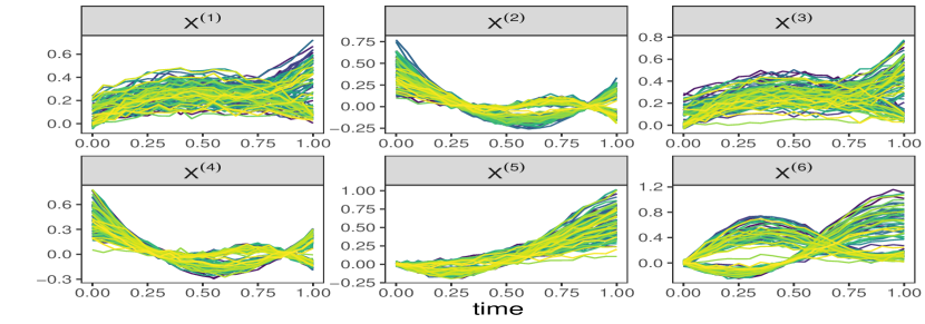
The terms $G^{j}_{i}$ and $G^{\prime j}_{i}$ allow to randomly affect typical temporal behaviors, defined by $f_{j,1}$ and $f_{j,2}$ functions, to observations. The $\beta_{i}$ and $\beta^{\prime}_{i}$ are dilatation/shrinkage terms of $f_{j,1}$ or $f_{j,2}$, while $W_{i}^{1}(t)$ corresponds to an additive noise. As illustrated in Figure 1, for each input variable, the observed trajectories are variations of the typical temporal behavior functions. The observations are divided into two groups of trajectories.

Figure 1: Dynamics of $n=100$ simulated input trajectories according to the model (18)

.

Output variable $Y$ is simulated in a similar way. The pair $(G_{i}^{1},G_{i}^{2})$ is used to determine a trajectory for the output variable, this is the primary link between $X_{i}$ and $Y_{i}$

$$Y_{i}(t)=\beta_{i}\sum_{j=1}^{2}\sum_{k=1}^{2}g_{j,k}(t)\mathbb{1}_{\{G^{j}_{i}=j-1\}}\mathbb{1}_{\{G_{i}^{k}=k-1\}}+W_{i}^{2}(t)$$ (19)

where $Y_{i}(t)$ is the $i$th output curve measured at time $t$; $t$ browses the same subdivision as in (18), $\beta_{i}$ are the same coefficients used in (18), $W_{i}^{2}\left(t\right)$ is a Gaussian white noise with standard deviation $0.05$ and $g_{j,k}$ are given by:

$$\left\{\begin{array}[]{l@{\hskip 5ex}l}g_{1,1}(t)=t+0.3\sin(10\left(t+1\right))\hfil\hskip 21.52771pt\\ g_{1,2}(t)=t+2(t-0.7)^{2}\hfil\hskip 21.52771pt\\ g_{2,1}(t)=1.5\exp\left(-\frac{(t-0.5)^{2}}{0.5}\right)-0.1\left(t+1\right)\cos(10t)\hfil\hskip 21.52771pt\\ g_{2,2}(t)=\frac{\log(13(t+0.2))}{1+t}\hfil\hskip 21.52771pt\\ \end{array}\right.$$ (20)

The response curves are distributed according to four different trajectory shapes, one for each pair of possible trajectory shapes for the first two input curve variables $X^{(1)}$ and $X^{(2)}$. Of note, the variables $X^{(3)}$ and $X^{(4)}$ are simulated using the same temporal functions as variables $X^{(1)}$ and $X^{(2)}$; however, the trajectories of variables $X^{(3)}$ and $X^{(4)}$ are simulated from $G^{\prime j}$ and not from $G^{j}$ and thus have no relation with the output variable $Y$.

5.2 Second scenario, predict curves with images, scalars and curves

In this scenario, we want to predict output curves from inputs that are curves, scalars and images to illustrate the flexibility of the Fréchet RF method, in particular its ability to learn about different types of inputs and outputs. The input curve variables are simulated according to the model (18) of the first scenario with $\beta_{i}$ and $\beta_{i}^{\prime}$ drawn according to $\mathcal{N}(1,1)$ in order to have large variations of the curves around their average temporal behavior. Similarly, the output curves are simulated according to the model (19) of the first scenario. Let $\left(\mathcal{M}^{1}_{i}\right)_{i}$ and $\left(\mathcal{M}^{2}_{i}\right)_{i}$ two sequences of handwritten images of numbers 1 (for $\mathcal{M}^{1}_{i}$) and 2 (for $\mathcal{M}^{2}_{i}$) randomly drawn from the MNIST dataset [LeCun and Cortes, 2010]. We simulate two input image variables $I^{(1)}$ and $I^{(2)}$ according to the following model:

$$I^{(j)}_{i}=\mathcal{M}^{1}_{i}\mathbb{1}_{\{G^{j}_{i}=0\}}+\mathcal{M}^{2}_{i}\mathbb{1}_{\{G^{j}_{i}=1\}}\quad\mbox{for}\ j\in\{1,2\};\ i\in\{1,\ldots,n\}$$ (21)

where $G^{j}_{i}$ are the same draws as those used to simulate the input and output curves in model (18) and model (19). Finally, consider the two real input variables $R^{(1)}_{i}=\beta_{i}$ and $R^{(2)}_{i}=\beta_{i}^{\prime}$, where the $\beta_{i}$ and $\beta_{i}^{\prime}$ are the same as those used to simulate the input and output curves. The first variable $R^{(1)}$ determines the intensity of the contraction/expansion of the $X^{(1)}$ and $X^{(2)}$ response curves. It is important to note that the link between the output curves and the input variables is entirely contained in the pairs $(G^{1}_{i},G_{i}^{2})$ which determine the general shape of the output curve as well as the $\beta_{i}$ which determine the compression/expansion of the output curves. The pairs $(G^{1}_{i},G_{i}^{2})$ as well as the $\beta_{i}$ are used to simulate the first two curve input variables $X^{(1)}$ and $X^{(2)}$. However the two image variables are constructed only from the pairs $(G^{1}_{i},G_{i}^{2})$ and the scalar variables are $\beta_{i}$ and $\beta_{i}^{\prime}$.

5.3 Third scenario, predict images with curves, a toy example

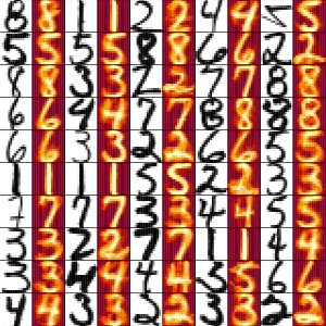
The purpose of this scenario is to illustrate the ability of the Fréchet RF method to predict images from input curves. We simulate a dataset of $n=500$ observations, the input curve variables are simulated according to the model (18) of the first scenario. As in the second scenario, the output images are taken from the MNIST dataset [LeCun and Cortes, 2010]. For any $k=1,\ldots,8$ and for any $i=1,\ldots,n$ we note $\mathcal{M}_{i}^{k}$ the random draw of the handwritten $k$ digit in the MNIST dataset for the $i$th observation. Let the pair $(G_{i}^{1},G^{2}_{i})$ used to attribute their shape to the curves of the first two input variables for the $i$th observation and $\beta_{i}$ the expansion/contraction parameter of these same curves, then the output images are drawn according to the combinations summarized in the Table 1.

	$G^{1}_{i}=0,\ G_{i}^{2}=0$	$G^{1}_{i}=1,\ G_{i}^{2}=0$	$G^{1}_{i}=0,\ G_{i}^{2}=1$	$G^{1}_{i}=1,\ G_{i}^{2}=1$
$\beta_{i}>1$	$\mathcal{M}_{i}^{1}$	$\mathcal{M}_{i}^{3}$	$\mathcal{M}_{i}^{5}$	$\mathcal{M}_{i}^{7}$
$\beta_{i}\leq 1$	$\mathcal{M}_{i}^{2}$	$\mathcal{M}_{i}^{4}$	$\mathcal{M}_{i}^{6}$	$\mathcal{M}_{i}^{8}$

Table 1: Random draws in the MNIST dataset of the output images from the realizations $G^{1}_{i},\ G^{2}_{i}$ and $\beta_{i}$ used to simulate the input curves.

As in the first scenario, the output images depend only on the first two input variables, the link between the images and the curves is entirely contained in the pairs $(G_{i}^{1},G_{i}^{2})$ as well as in the $\beta_{i}$. This means that the handwritten number images then depend both on the shape of the curves of the first two input variables and their amplitude.

5.4 Results

5.4.1 First scenario

First, we need to determine a metric for each input and output space. In the case of longitudinal data i.e. when repeated measurements of quantitative variables are available over time. The observations for $p$ input and one output variables can thus be represented by time-dependent curves. In this case, the $i$-th observation $X_{i}$ is a curve from $\mathcal{I}_{1}\times\cdots\times\mathcal{I}_{p}\subset\mathbb{R}^{p}_{+}$ to $\mathbb{R}^{p}$ (where $\mathcal{I}_{1}=[0,1]$ and $\mathcal{I}_{2}=[0,1]$ in the first scenario), and $Y_{i}$ is a curve from $\mathcal{J}\subset\mathbb{R}_{+}$ to $\mathbb{R}$. We choose to equip the resulting curves spaces with the Fréchet distance $d_{\mathcal{F}}$ introduced in [Fréchet, 1906] defined for two real-valued curves $f$ and $g$ with support in $\mathcal{I}\subset\mathbb{R}_{+}$ as

$$d_{\mathcal{F}}(f,g)=\inf_{\alpha,\beta}\max_{t\in\mathcal{I}}|f(\alpha(t))-g(\beta(t))|$$

where $\alpha$ and $\beta$ are any re-parameterizations of $\mathcal{I}$. The definition is the same in the discrete case (polygonal curves), except that $t$ takes values on $\mathcal{I}$ by intervals, see [Alt and Godeau, 1995] for a full description of Fréchet distance for discretely sampled curves. This distance is a natural measure of similarity between the shapes of curves and has been widely used in various applications such as signature authentication [Zheng et al., 2008], path classification [Genolini et al., 2016] and speech recognition [Kwong et al., 1998]. Note that, unlike several classical distances, the calculation of the Fréchet distance does not require the same number of measurements, nor the same observations times on the two trajectories. Once we have determined the metrics used for the different spaces we need to define the split function used to cut on the input spaces. Finally, the 2-means algorithm for longitudinal data using Fréchet distance and Fréchet mean introduced in [Genolini et al., 2016] is chosen on each input space to determine the different competing splits. This split function called kmlShape is an adaptation of the $k$-means method tailored to one-dimensional curves. It allows to find groups of trajectories based on their shapes (which are usually not found by conventional methods, e.g. based on Euclidean distance).

Fréchet trees and Fréchet random forests were compared on simulated datasets to standard CART trees [Breiman et al., 1984] and standard random forests [Breiman, 2001] as well as standard existing methods for longitudinal data analysis such as linear mixed effects model (LMEM) with a random intercept and a random effect on time and the boosting functional regression method FDboost [Brockhaus et al., 2017] with optimized number of iterations.

The prediction errors (mean squared error) of all the methods are estimated on several sample sizes $n=100,\ 200,\ 400$ and 1000 using for each sample size, $100$ datasets simulated according to models (18) and (19). For each simulated dataset $\mathcal{L}_{n}$, we randomly divide $\mathcal{L}_{n}$ into a training set (with $0.8n$ observations) and a test set (made of the remaining $0.2n$ observations). The Fréchet distance is used on the curved input and output spaces to build Fréchet trees and Fréchet random forests, however in order not to advantage our method, prediction errors are calculated with the usual $L^{2}$ Euclidean distance (time by time) which benefits to the standard approaches like CART trees, RF and FDboost.

Figure 2: Boxplots of the prediction error of the Fréchet random forests method according to the mtry parameter. Prediction errors are calculated on 100 datasets of size $n=100$ simulated according to models (18) and (19) of the first scenario.

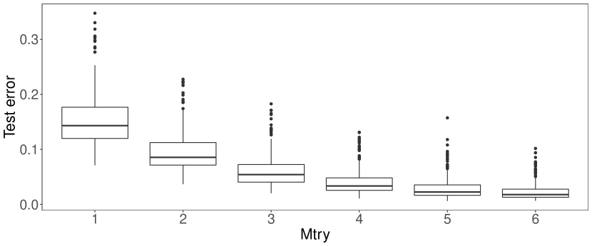
The number of randomly drawn variables mtry at each node has usually a strong impact on random forests performance: if mtry is too small, individual trees would give too poor predictions, and if mtry is too high, the collection of trees could be not diverse enough ([Díaz-Uriarte and Alvarez De Andres, 2006];[Genuer et al., 2008]). As illustrated in Figure 2 the prediction error (MSE) of the Fréchet random forest decreases as the value of the mtry increases. In all our experiments in the first scenario, we chose mtry=5. We set the number of trees $q$ to $250$ (justified by the fact that, in this experiment, the OOB error stabilizes as soon as $100$ trees are included in the forest). The standard random forest was composed of 500 trees and the mtry parameter was otpimized to 2. The number of iterations for FDboost is selected between 1 and 500 through the internal procedure of the package.

Figure 3: Boxplots of the prediction error (MSE) of the Linear mixed effects model (LMEM), CART tree, random forests (RF), FDboost, Fréchet tree (Ftree) and Fréchet random forest (FRF) methods estimated on 100 datasets simulated according to the simulation scheme of the first scenario for $n=100,\ 200,\ 400$ and $1000$ sample sizes.

Figure 4: Boxplots of the prediction error (MSE) and computation times estimated over 100 datasets of sample size $n=100$ simulated under models (18) and (19) for Fréchet RF (FRF) method and Extremely Randomized Fréchet RF (ERFRF) method with different values of ntry.

As illustrated in Figure 3 for any sample size, FDboost, Fréchet tree, and Fréchet random forests clearly outperform the standard LMEM, CART and RF methods. Not surprisingly, the transition from a Fréchet tree to a Fréchet RF greatly improves predictive capacity by reducing prediction error and error variance. For instance, when $n=100$, the estimated MSE obtained with a Fréchet tree is 0.047 while the one obtained with a Fréchet RF is 0.028 which is a 40% decrease in prediction error. Even though FDboost (our principal competitor) shows very good performances, Fréchet tree and Fréchet RF are the methods that obtain the lowest prediction errors for all sample sizes. More precisely, for small dataset ($n=100$) FDboost obtains an estimated MSE of 0.05 while Fréchet tree and Fréchet RF obtain respectively 0.047 and 0.028 while for large dataset ($n=1000$) the estimated MSE of FDboost is 0.031 and the Fréchet tree and Fréchet RF estimated MSE are respectively 0.012 and 0.006. Finally, note that the prediction error of the FDboost, Fréchet tree and Fréchet RF methods decreases as the sample size $n$ increases which is not the case with other methods that keep a stable prediction error. Additionally, this decrease is much larger with the Fréchet tree and Fréchet RF methods than with the FDboost method. Moreover, the error prediction of the Fréchet RF converges to zero as $n$ tends to infinity.

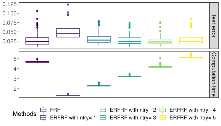
The extremely randomized version of Fréchet random forests introduced in Section 3.3 has some advantages over the Fréchet RF method. In particular, they are easy to implement, can be used for any type of data and reduce calculation times. In order to verify this claim we calculate the prediction error obtained by extremely randomized Fréchet forests (ERFRF) for different values of ntry on 100 data sets of size $n=100$ simulated according to the first scenario. As shown in Figure 4, the prediction error of the ERFRF method decreases as the value of the ntry increases. When ntry is large enough (here ntry=3), the error obtained by ERFRF is similar to that obtained by Fréchet RF. Moreover, the execution time of an ERFRF is much lower than that of a Fréchet RF. For example, the build time of an Fréchet RF is 281 seconds while the build time of an ERFRF with ntry=3 is 191 seconds which is 30% lower. Similar results are obtained on larger datasets (not shown here).

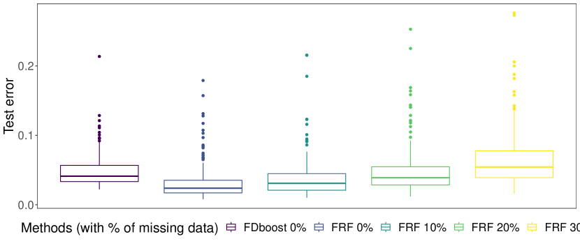
As mentioned in the presentation of the Fréchet distance at the beginning of this section, using the Fréchet distance allows to calculate the distance between two curves measured at different times. Thus, having missing observation times for some curves does not prevent the construction of the trees, as long as not all observation times are missing for a given curve. In order to study the robustness of Fréchet RF to missing observations, we simulate new datasets with $n=100$ individuals according to models (18) and (19) by randomly removing 10%, 20% and 30% of the observation times for each curve. It is important to note that the removed observation times are different for each curve. For example, the observations removed for the first variable of the first individual will not necessarily be the same as those removed for the second or third variable or even the output curve of the same individual. It is then impossible to use the standard LMEM, RF and FDboost methods (it is always possible to use the CART method by removing the missing observations for the output curves). As shown in Figure 5, the prediction error obtained by Fréchet RF increases slightly as the percentage of missing observations increases. Moreover, the prediction error obtained with Fréchet RF on simulated data sets with 30% missing data remains competitive with that obtained by the FDboost method on datasets without missing observations.

Figure 5: Boxplots of the estimated prediction error over 100 datasets of sample size $n$=100 simulated under models (18) and  (19) for FDboost and Fréchet RF (FRF) methods based on the number of missing observations.

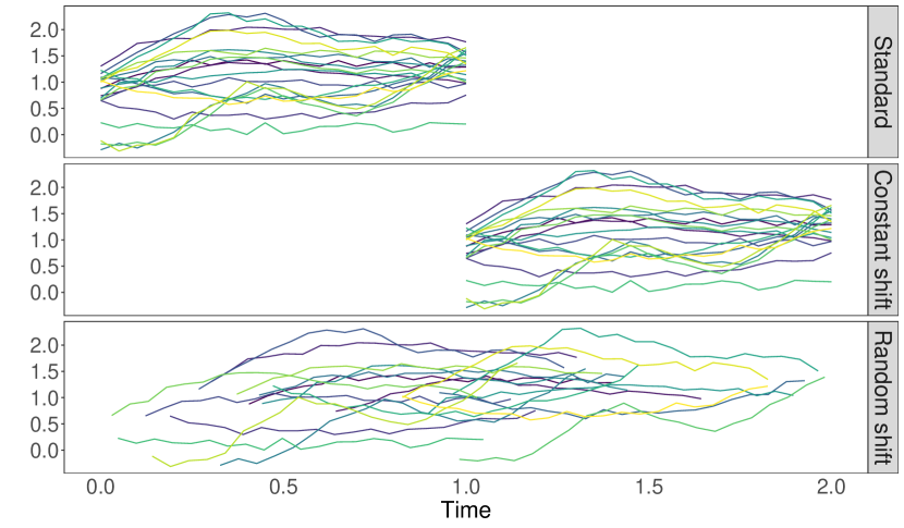
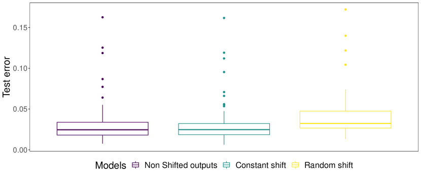
It is rather common in biostatistical applications and more particularly in clinical trials to have a response variable observed after the measurement times of the input variables, this is the case of our application on DALIA-I vaccine trial (see Section 6). In order to study the stability of Fréchet RF method to time shifts, we transform the output curves by shifting them: i) by the same time shift of 1 for all the curves, i.e., the output curves are observed on windows $[1,2]$ instead of $[0,1]$ (keeping the same shapes); ii) by randomly shifting each of them according to a uniform $\mathcal{U}([0,1])$, making the windows of observation of the output curves all different in this case (see Figure 6 for the simulated dynamics according to the time shifts). As illustrated in Figure 7, the constant time shift for the response curves has no influence on the Fréchet RF prediction error. When the offsets are randomly drawn for each output curve, the prediction error increases slightly to an average error of 0.039, however note that this error is still 20% smaller than the average error of 0.05 obtained by FDBoost on simulated data without time shifts.

Figure 6: Dynamics of the output variable curves simulated according to the model (4) in the standard case (i.e. without time shift), with a constant time shift equal to 1; with a uniform time shift $\mathcal{U}([0,1])$.

Figure 7: Boxplots of the estimated prediction error over 100 data sets of size $n$=100 simulated under the second scenario for the FDboost methods based on the time shift applied to the output curves.

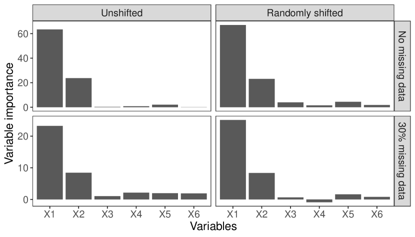
Finally, Figure 8 gives the importance scores of variables calculated with the Fréchet RF method on 4 datasets of size $n=100$ simulated according to models (18) and (19):

1. With no time shifts on the output curves and no missing observation times.

2. With random time shifts according to a uniform $\mathcal{U}([0,1])$ on the output curves but with no missing measurement times.

3. With no time shifts but with 30% missing observation times.

4. With 30% missing observations and time shifts on the output curves.

This graph shows that neither time shifts nor missing observation times have an impact on the importance of the variables. In fact, the first two variables (those related to the output variable) are always the ones with the highest importance scores. The other four variables (unrelated to the output variable) have extremely low importance scores compared to the first two variables.

As a conclusion, we illustrate the superiority on longitudinal data (in terms of prediction error) of the Fréchet trees and Fréchet RF methods compared to the standard LMEM, CART, RF methods as well as the longitudinal boosting method FDboost. In addition, we illustrate the great robustness of the method to missing data and time shifts, both in terms of prediction error and the importance of the variables. Lastly, we show that the extremely randomized variant ERFRF can obtain a prediction error similar to that of Fréchet RF while having lower computation times, making it a method of choice for analyzing very large datasets.

Figure 8: Barplots of the Fréchet RF variable importance scores, obtained on 4 datasets simulated according to model (18) and model (19). The results in the left-hand column are obtained on the simulated datasets without time shift while the right-hand column contains those obtained with a random time shift on the output curves. The results on the first row are those obtained on the simulated data sets without missing data while those on the second row are those obtained on the simulated data sets with 30% missing data on the input and output curves.

5.4.2 Second scenario

The Fréchet distance is used on curve spaces while the standard Euclidean distance is used on scalar spaces and image variables. Since there is no comparison with other methods in this scenario, the OOB error will be used as a measure of the performance of the Fréchet RF. Throughout this section we study the ERFRF method, the version implemented in our package FrechForest that can handle images and shapes as inputs.

Figure 9: Examples of 4 extremely randomized trees of depth 2 built on $n=100$ simulated observations according to the second scenario. The 4 trees are constructed from the input variables of: 1) scalars only; 2) curves only; 3) images and scalars; 4) curves, images and scalars. Below each node is indicated the split variable. To the left and right of each node are indicated the representative elements of the right and left child nodes for the split variable in question. For example for model 3) the split variable of the root node is $I^{(2)}$, the images of the variable $i^{(2)}$ which are closer to the image on the left (for the Euclidean distance), a blurred 2, go into the node $t_{2}$ while those closer to 1 go into the node $t_{3}$.

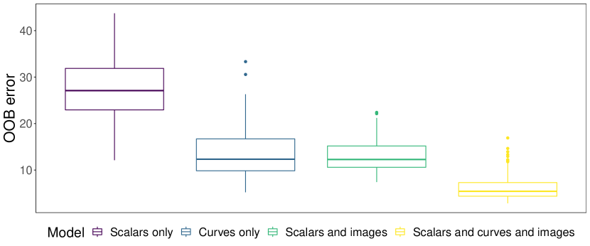
We study the OOB error obtained by ERFRF according to the types of input variables (images, curves or scalars) on 100 datasets of size $n=$100 simulated according to the second scenario. We consider the following models:

1. Only scalar variables $R^{(1)}$ and $R^{(2)}$ are used to predict output curves.

2. Only curve variables $X^{(1)},\ldots,X^{(6)}$ are used to predict output curves.

3. Image variables $I^{(1)}$ and $I^{(2)}$ and scalar variables are used.

4. all variables i.e. curves, scalars and images are used to predict output curves.

Note that case 2 corresponds to the first simulation scenario. Figure 9 shows an example of an extremly randomised Fréchet tree of depth 2 (only the first three splits are shown here) for each model above. When the models incorporate different types of inputs, in the case of models 3) and 4), the constructed trees are mixed in the sense that they can alternate the split spaces. For example, in the case of model 4), Figure 9 shows an example of a tree with the first three splits in the three different types of input spaces: curves, scalars and images. The parameters mtry and ntry are selected for each model to minimize the OOB error of the ERFRF, and are therefore different for each model.

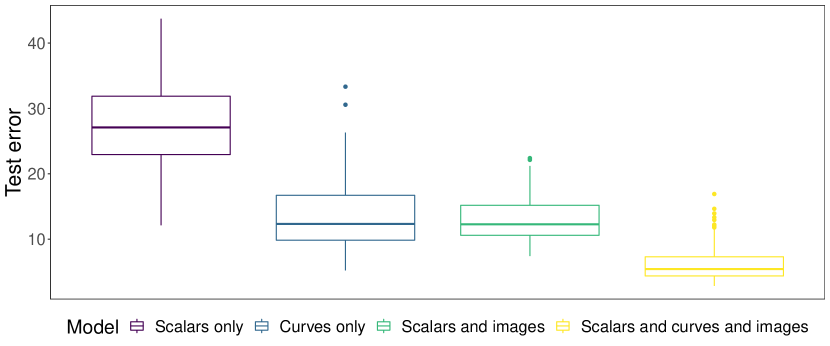
As shown in Figure 10, the highest OOB error is obtained when only scalar variables are used. When the image variables are added to the scalar variables, the OOB error is the same as the one obtained on the model using only the input curves. This was expected since the input curve variables provide the same information as the image and scalar variables combined. More precisely, the input curve variables provide both information on the shape of the output curves as well as on their amplitude, whereas the information on the shape is only provided by the images and the ones on the amplitude is only provided by the scalars. Individually, the input variables of images or scalars provide only part of the information that is provided by the input variables of curves. Finally, when the image and scalar variables are added to the curve variables, the OOB error of the ERFRF decreases. This is explained by the fact that in some cases, when the contraction or dilation of the input curves is too large, the dilated or contracted curves may have a very different shape than their initial shape and thus lose the information they brought due to their shape. Thus the addition of image variables allows to always have access to information on the shapes of the output curves. Finally, the results of these simulations emphasizes the main strength of the ERFRF method, which is to handle heterogeneous data, i.e. input and output variables of different natures.

Figure 10: OOB errors of the ERFRF method according to the types of input variables. The OOB errors are obtained on 100 data sets of size $n=100$ simulated according to the second scenario.

5.4.3 Third scenario

The Fréchet distance is used on the curve spaces, i.e. on the 6 input variables. The distance used on the output space is the standard Euclidean distance. A Fréchet RF is constructed with $q=500$ trees (justified by the fact that the OOB error of the Fréchet RF becomes stable as long as 350 trees compose the forest). Similarly, the mtry parameter is set to 5. As shown in Figure 11, OOB predictions of output images always give the correct written digit. However, ghosting can be seen on some digit predictions. This is due to the simulation scheme itself. The input curves only give information about the written number, and do not provide any information about its individual characteristics such as the width of the number, its height, the presence or not of a loop (for writing a 2 for example). More precisely, there is within the same group of numbers (for example the set of numbers 4 drawn) a variability in the written numbers that is not explained by the input curves. By introducing variables that provide information on the fine characteristics of each written number (such as its height, width, etc.) we would get even more accurate predictions. Moreover, it is noticeable that this phenomenon of ghosting is not present for numbers that have a very low variability in their writing such as the number 1. In order to highlight this point a Fréchet RF is constructed on the same simulated dataset and the images are replaced by factors indicating what the written number is. When the outputs are images, the percentage of explained variance is 20%, which was expected since there is a large variability between the same numbers that is not explained by the input curves. When the outputs are factors expressing the written numbers, the percentage of explained variance is 98%. It is therefore clear that the link between the output images and the input curves relates only to the digits and not to its individual characteristics. So even if the explained variance percentage is only 20% for the images, the Fréchet RF (almost) always predicts the right digit.

Figure 11: True output images and OOB predictions. In black and white (grayscale), 50 output images from the dataset of $n=500$ observations simulated according to the third scenario are displayed. The redscale image to the right of each grayscale image is the OOB prediction given by the trained Fréchet RF.

6 Application to real data

6.1 DALIA vaccine trial

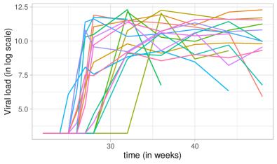
DALIA is a therapeutic vaccine trial including 17 HIV-infected patients who received an HIV vaccine candidate before stopping their antiretroviral treatment. For a full description of the DALIA vaccine trial we refer to [Lévy et al., 2014]. At each harvest time before stopping their treatment, 5,399 gene transcripts which significantly vary over time during the vaccination phase were selected by [Hejblum et al., 2015] among more than 32000. The plasma HIV viral load (which was log-transformed) for every patient was measured at each harvest time after the antiretroviral treatment interruption (called HAART interruption). In this application the measurement times of the inputs (gene transcripts) differ from the ones of the output (HIV viral load). The objective is to be able to predict the HIV viral load dynamics after antiretroviral treatment interruption for a patient given the evolution of his/her gene expression during the vaccination phase [Thiébaut et al., 2019]. Figure 12 illustrates the design of the DALIA vaccine trial and the dynamics of the viral replication after antiretroviral treatment interruption with a large between-individuals variability. The analysis with Fréchet random forest was performed on the 17 patients. The $mtry$ parameter was fixed to $1500$ and the number of trees, $q$, was set to $500$. The OOB error of the Fréchet random forest converged and stabilized for almost $100$ trees composing the forest. Figure 13 illustrates both the OOB predictions and the predictions on the learning samples (fits) of the evolution of the viral load after the HAART interruption for 4 patients of the vaccine trial.

Figure 12: On the left, the vaccine trial design. On the right, dynamics of plasma HIV viral load (one curve per patient) after antiretroviral treatment interruption (from week 24 to week 48), DALIA vaccine trial.

Figure 13: Viral load after antiretroviral treatment interruption as a function of time, for four patients, together with both OOB predictions and fits (predictions on learning samples) obtained by Fréchet random forests, DALIA vaccine trial.

The predictions of the Fréchet forest on the learning sample were close to the observed viral load curves. Moreover, despite a very small number of individuals, the OOB predictions obtained with this forest are quite close in shape to the true curves.
Among the 100 most important variables, many belong to the groups of genes (modules) that were selected in [Thiébaut et al., 2019] because i) their dynamics was influenced by the vaccine ii) their abundance after vaccination were associated with the maximum of the observed viral load. For instance, five genes from the inflammation module 3.2 and three genes from the T cell module 4.1 were selected with the current approach. Both groups of genes were extremely relevant in the context of such vaccine that generates strong T cell response.
Thus, the Fréchet random forests method applied on the complex example of the DALIA vaccine trial is extremely effective both for its capacity to predict the output variable as well as for its ability to find relevant genes in order to explain the evolution of the viral load after the treatment interruption. Previous analyses performed in [Thiébaut et al., 2019] were done by looking at the association between one time of measurement for the input gene expressions and only one characteristic of the viral load dynamics: its maximum value. The Fréchet random forest allows a direct analysis of the whole longitudinal information available. It should be noted that standard CART trees and random forests methods cannot be used on such an application. Indeed, both the number and the observation times of the input and output variables were different.

6.2 LIGHT vaccine trial

LIGHT is a therapeutic vaccine trial including 97 HIV-infected patients. Using the data available in this trial, the objective of the present analysis was to assess the capacity of predicting the abundance of CD4 T cells using gene expression data as measured by RNA sequencing in whole blood, dealing with high-dimensional longitudinal data with extremely unbalanced trajectories. The dataset is composed by 1150 input variables of genes abundance. Those 1150 input genes were preselected using dearseq [Gauthier et al., 2019], a method for differential expression analysis. These are found to be differentially expressed overtime among more than 17000 genes. A targeted control rate for the False Discovery Rate was used at a nominal level of 5%.
Furthermore, there were 234 observations in the dataset: one to four measurements were available for each patient. In Section 5.4.1 we showed that the Fréchet RF method was very robust to unbalanced experimental designs. However, in the LIGHT dataset there is a significant proportion of patients with only one observation time, which is an extreme case that can cause some problems in predicting trajectories with three or four measurement times. We then consider the output as scalars, i.e. all the output observations are independent. We used 4 different RF models:

1. A standard RF.

2. A Fréchet RF considering the inputs as scalars.

3. A Fréchet RF considering the inputs as curves.

4. A Fréchet RF considering both the inputs as curves and as scalars.

As in our simulations, the Fréchet distance is used for curve spaces while the Euclidean distance is used for scalar spaces. For each random forest model the mtry parameters as well as the number of trees composing the forest are optimized to minimize the OOB error. The prediction error estimated on OOB samples for the different RF models are compared. The standard RF method as well as the Fréchet RF method with inputs and outputs treated as scalars obtain the highest OOB errors with 22.65 and 22.61 respectively. When the input is treated as curves, the Fréchet RF method obtains an OOB error of 17.59 which represents a decrease of more than 20% of the OOB error compared to the first two models. Unsurprisingly, and in line with our simulations, considering repeated observations from the same patient as curves and partitioning the input space according to the shape of these curves greatly improves predictive performance. When the inputs are treated as both curves and scalars, the prediction error obtained from the Fréchet RF is 17.36. Thus, adding the same input variables considered as scalars does not improve the OOB error already obtained by the Fréchet RF on the curve variables only. Genes as scalars (i.e. when all observations are independent) do not therefore provide additional information compared to genes as curves, because integrating these genes in the form of scalars does not improve the prediction error.

Figure 14: Importance scores of the 200 most important input genes calculated with the RF Fréchet, in LIGHT vaccine trial.

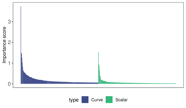
Finally, the importance scores of the variables are considered. Figure 14 shows the importance scores of the 200 most important input genes calculated with the RF Fréchet built on the genes considered as curves as well as scalars. The genes as curves globally obtain much higher importance scores than those obtained by the genes as scalars. A closer analysis of the importance scores of genes according to their type (curve or scalar) shows that the importance score for a gene as curve is systematically higher than that obtained by the same gene as a scalar. Moreover, of the 200 genes in curve form that obtain the highest importance scores, less than 47% are common to the 200 most important genes for genes in scalar form. To go further, only 42% of the 200 genes in the form of curves that obtain the highest importance scores are common to the 200 most important genes found with the standard RF method. Thus, in the LIGHT vaccine trial, considering the observations from the same patient as a trajectory not only greatly improves the prediction error but also allows us to find genes that were not previously found with the standard RF method. From the importance scores of the variables we selected the 100 most important genes for the genes considered as curves. Among these 100 genes, many of them (e.g. CD8A, CD40, TLR3, TRBV1, TRBV18…) were completely related to T cell pathways as expected because they are associated to the abundance of CD4+ T cells. Hence, Th1 pathway, Th2 pathway, T cell exhaustion pathways were among the most enriched pathways among the 100 selected genes (Ingenuity Pathway Analysis). Interestingly, the genes and pathways associated to the analysis considering inputs as scalar were less relevant with for instance the absence of the genes associated to communication between immune cells (CCL4, CCL5, CCL7) that were selected when taking into account the curves. Finally, the RF Fréchet considering the repeated measures as curves provided very relevant gene selection in this application.

7 Discussion

Two new tree-based methods, Fréchet trees and Fréchet random forests, for general metric spaces-valued data were introduced. Let us emphasize that the proposed methods are very general. Indeed, input variables can thus all be of different kinds, each one having its own metric, and the kind of the output variable can also be a different one.

The example of learning curve shapes in the context of longitudinal data was presented to illustrate the capacity of the methods to learn from data in unordered metric spaces. A simulation study in this framework demonstrated the superiority of Fréchet trees and forests over the existing classical methods, both in terms of prediction error as well as robustness and flexibility. An important aspect highlighted in our study is the great robustness of Fréchet trees and Fréchet random forests. Indeed, our simulations illustrated the ability to handle missing data as well as different observation times for the different variables, which is common in longitudinal datasets. Two other simulation scenarios demonstrated the capacity of the methods to simultaneously handle data of different natures such as curves, images, scalars, factors, shapes etc. This great flexibility allows the construction of more efficient predictors while being able to compare the information provided by each of these variables of different natures thanks to the importance score. In this article, we analyzed two high-dimensional longitudinal datasets from vaccine trials. For the first time and due to the very high flexibility of Fréchet RF, it was possible to associate the entire evolution of the transcriptome during the vaccination phase with the entire evolution of the immune response after interruption of treatment on DALIA-I dataset. We have thus highlighted the groups of genes that best explain the different immune response after interruption of treatment. Finally, within the framework of LIGHT vaccine trial on which the classical methods stumbled, we highlighted the superiority of the Fréchet RF method. We illustrated that regression on curve shapes could greatly improve the prediction error while selecting new variables.

However, there are two main limitations to Fréchet trees and forests: the first one is that the Fréchet mean has to exist in the output space [Le Gouic and Loubes, 2017] and has to be fairly approximated. The second concerns the computation time. Indeed, even if the proposed approaches have been fully coded in the R package FrechForest for the trajectories case, Fréchet random forests can still be computationally intensive. This problem can be alleviated by the fact that, as all forests methods, they are easily parallelized (the different trees can be built in parallel).

Finally, we are working on the rates of convergence of Fréchet trees and Fréchet random forests. In parallel, we are working on the efficient implementation of metrics adapted to the image problem, such as the Wassertein distance [Vallender, 1974], in order to apply the Fréchet RF method to large brain imaging databases.

Appendix A Proof of Theorem 14

First, we demonstrate the point-wise consistency given by (13). We introduce the following quantity

$$r_{n}\left(x,y\right)=\frac{\frac{1}{n}\sum_{i=1}^{n}d^{2}(Y_{i},y)\mathbb{1}\{X_{i}\in\pi_{n}[x]\}}{\mathbb{P}\left(X\in\pi_{n}[x]\right)}$$ (22)

From 11 we have $T_{n}(x)=\underset{y\in\mathcal{Y}}{\operatorname*{arg\,min}}\ r_{n}\left(x,y\right)$. First, we use the following classical upper bound in $M$-estimation:

$$r\left(x,T_{n}(x)\right)-\underset{y\in\mathcal{Y}}{\min}\ r\left(x,y\right) =r\left(x,T_{n}(x)\right)-r_{n}\left(x,T_{n}(x)\right)+r_{n}\left(x,T_{n}(x)\right)-\underset{y\in\mathcal{Y}}{\min}\ r\left(x,y\right)$$

$$=r\left(x,T_{n}(x)\right)-r_{n}\left(x,T_{n}(x)\right)+r_{n}\left(x,T_{n}(x)\right)-r\left(x,\phi^{*}(x)\right)$$

$$\leq r\left(x,T_{n}(x)\right)-r_{n}\left(x,T_{n}(x)\right)+r_{n}\left(x,\phi^{*}(x)\right)-r\left(x,\phi^{*}(x)\right)$$

$$\leq 2\underset{y\in\mathcal{Y}}{\sup}\left|r_{n}\left(x,y\right)-r(x,y)\right|$$ (23)

We are going to decompose the above supremum in several terms that we are going to appropriately upperbound to obtain their decay to zero under the assumptions Theorem 14. Consider a $\delta$ covering of $\mathcal{Y}$ with centers $\{y_{\alpha}\}_{\alpha=1}^{Q}$ where $Q=N(\delta,\mathcal{Y},d)$. Thus, for every $y\in\mathcal{Y}$, there is $\alpha=\alpha_{y}\in\{1,\ldots,Q\}$ such as $d\left(y,y_{\alpha}\right)<\delta$. We introduce the following quantity

$$r^{E}\left(x,y\right)=\frac{\mathbb{E}\left(d^{2}(Y,y)\mathbb{1}\{X\in\pi_{n}[x]\}\right)}{\mathbb{P}\left(X\in\pi_{n}[x]\right)}$$ (24)

Then, the following decomposition is used

$$r_{n}\left(x,y\right)-r(x,y)=\underbrace{r_{n}\left(x,y\right)-r_{n}\left(x,y_{\alpha}\right)}_{(i)}+\underbrace{r_{n}\left(x,y_{\alpha}\right)-r^{E}\left(x,y_{\alpha}\right)}_{(ii)}\\ +\underbrace{r^{E}\left(x,y_{\alpha}\right)-r^{E}\left(x,y\right)}_{(iii)}+\underbrace{r^{E}\left(x,y\right)-r\left(x,y\right)}_{(iv)}$$ (25)

We are now going to derive upper bounds for each of the four terms above that do not depend on $y$. Let us start with the term $(i)$ of (25), we introduce the following event

$$\mathcal{E}_{n}=\left\{\left|\frac{\frac{1}{n}\sum_{i=1}^{n}\mathbb{1}\{X_{i}\in\pi_{n}[x]\}}{\mathbb{P}\left(X\in\pi_{n}[x]\right)}-1\right|<\frac{1}{2}\right\}.$$

We can upper bound the probability of the complementary of the event $\mathcal{E}_{n}$ (denoted $\mathcal{E}_{n}^{c}$) as

$$\mathbb{P}\left(\mathcal{E}_{n}^{c}\right) =\mathbb{P}\left(\left|\frac{\frac{1}{n}\sum_{i=1}^{n}\mathbb{1}\{X_{i}\in\pi_{n}[x]\}}{\mathbb{P}\left(X\in\pi_{n}[x]\right)}-1\right|>\frac{1}{2}\right)$$ (26)

$$\leq\mathbb{P}\left(\underset{\pi\in\Pi_{n}}{\sup}\underset{A\in\mathcal{\pi}}{\sum}\left|\frac{\frac{1}{n}\sum_{i=1}^{n}\mathbb{1}\{X_{i}\in A\}}{\mathbb{P}\left(X\in A\right)}-1\right|>\frac{1}{2}\right)$$ (27)

Then, we upper bound the last probability using Lemma 1

$$\mathbb{P}\left(\underset{\pi\in\Pi_{n}}{\sup}\underset{A\in\mathcal{\pi}}{\sum}\left|\frac{\frac{1}{n}\sum_{i=1}^{n}\mathbb{1}\{X_{i}\in A\}}{\mathbb{P}\left(X\in A\right)}-1\right|>\frac{1}{2}\right)\leq 4\Delta_{n}^{*}(\Pi_{n})2^{\mathcal{C}(\Pi_{n})}\exp-\frac{n}{128}$$ (28)

On the event $\mathcal{E}_{n}$, one has that $\left|\frac{\frac{1}{n}\sum_{i=1}^{n}\mathbb{1}\{X_{i}\in\pi_{n}[x]\}}{\mathbb{P}\left(X\in\pi_{n}[x]\right)}\right|<\frac{3}{2}$ which implies that

$$\left|r_{n}\left(x,y\right)-r_{n}\left(x,y_{\alpha}\right)\right|=\left|\frac{\frac{1}{n}\sum_{i=1}^{n}\left(d^{2}(Y_{i},y)-d^{2}(Y_{i},y_{\alpha})\right)\mathbb{1}\{X_{i}\in\pi_{n}[x]\}}{\mathbb{P}\left(X\in\pi_{n}[x]\right)}\right|\\ =\left|\frac{\frac{1}{n}\sum_{i=1}^{n}\left(d(Y_{i},y)-d(Y_{i},y_{\alpha})\right)\left(d(Y_{i},y)+d(Y_{i},y_{\alpha})\right)\mathbb{1}\{X_{i}\in\pi_{n}[x]\}}{\mathbb{P}\left(X\in\pi_{n}[x]\right)}\right|\\ \leq 2\operatorname*{diam}\left(\mathcal{Y}\right)d\left(y,y_{\alpha}\right)\left|\frac{\frac{1}{n}\sum_{i=1}^{n}\mathbb{1}\{X_{i}\in\pi_{n}[x]\}}{\mathbb{P}\left(X\in\pi_{n}[x]\right)}\right|\leq 3\operatorname*{diam}\left(\mathcal{Y}\right)\delta$$ (29)

On the complementary of the event $\mathcal{E}_{n}$, we use similar arguments and the upper bound $\left|\frac{\frac{1}{n}\sum_{i=1}^{n}\mathbb{1}\{X_{i}\in\pi_{n}[x]\}}{\mathbb{P}\left(X\in\pi_{n}[x]\right)}\right|\leq\frac{1}{\mathbb{P}\left(X\in\pi_{n}[x]\right)}$ to derive that

$$\left|r_{n}\left(x,y\right)-r_{n}\left(x,y_{\alpha}\right)\right|\leq 2\operatorname*{diam}\left(\mathcal{Y}\right)\delta\frac{1}{\mathbb{P}\left(X\in\pi_{n}[x]\right)}.$$

Therefore, we finally obtain that

$$\left|r_{n}\left(x,y\right)-r_{n}\left(x,y_{\alpha}\right)\right|\leq\operatorname*{diam}\left(\mathcal{Y}\right)\delta\left(3\mathbb{P}\left(\mathcal{E}_{n}\right)+2\frac{1-\mathbb{P}\left(\mathcal{E}_{n}\right)}{\mathbb{P}\left(X\in\pi_{n}[x]\right)}\right)$$

Now we consider the term $(ii)$ in (25). To this end, we propose to bound the following probability

$$\mathbb{P}\left(\underset{\alpha=1,\ldots,Q}{\max}\ \left|r_{n}\left(x,y_{\alpha}\right)-r^{E}\left(x,y_{\alpha}\right)\right|>\epsilon\right) =\mathbb{P}\left(\cup_{\alpha=1}^{Q}\left\{\left|r_{n}\left(x,y_{\alpha}\right)-r^{E}\left(x,y_{\alpha}\right)\right|>\epsilon\right\}\right)$$

$$\leq\sum_{\alpha=1}^{Q}\mathbb{P}\left(\left|r_{n}\left(x,y_{\alpha}\right)-r^{E}\left(x,y_{\alpha}\right)\right|>\epsilon\right)$$ (30)

For a fixed $\alpha\in\{1,\ldots,Q\}$, we define $W_{i}=\frac{d^{2}(Y_{i},y_{\alpha})\mathbb{1}\{X_{i}\in\pi_{n}[x]\}}{\mathbb{P}\left(X\in\pi_{n}[x]\right)}$, and we thus have that

$$r_{n}\left(x,y_{\alpha}\right)-r^{E}\left(x,y_{\alpha}\right)=\frac{1}{n}\sum_{i=1}^{n}W_{i}-\mathbb{E}\left(W_{i}\right),$$

which can be controlled thanks to Bernstein’s inequality by finding upper bounds on $|W_{i}|$ and $\operatorname*{var}(W_{i})$. To this end, we first derive a lower bound on $\mathbb{P}\left(X\in\pi_{n}[x]\right)$.

$$\mathbb{P}\left(X\in\pi_{n}[x]\right) =\mathbb{E}\left(\mathbb{P}\left(X\in\pi_{n}[x]\ |\mathcal{L}_{n}\right)\right)$$

$$=\mathbb{E}\left(\int_{\pi_{n}[x]}\rho_{X}(t)dt\right)\geq\rho_{\min}\mathbb{E}\left(\operatorname*{Vol}(\pi_{n}[x])\right)$$

$$=\rho_{\min}\mathcal{V}_{n}[x]\qquad\mbox{with}\quad\mathcal{V}_{n}[x]=\mathbb{E}\left(\operatorname*{Vol}(\pi_{n}[x])\right).$$

Therefore, we obtain that

$$|W_{i}|\leq\frac{d^{2}(Y_{i},y_{\alpha})\mathbb{1}\{X_{i}\in\pi_{n}[x]\}}{\rho_{\min}\mathcal{V}_{n}[x]}\leq\frac{\operatorname*{diam}^{2}\left(\mathcal{Y}\right)}{\rho_{\min}\mathcal{V}_{n}[x]}$$

Moreover,

$$\operatorname*{var}(W_{i})\leq\mathbb{E}\left(W_{i}^{2}\right)=\frac{\mathbb{E}\left(d^{4}(Y_{i},y_{\alpha})\mathbb{1}^{2}\{X_{i}\in\pi_{n}[x]\}\right)}{\mathbb{P}\left(X\in\pi_{n}[x]\right)^{2}}\leq\frac{\operatorname*{diam}^{4}(\mathcal{Y})\mathbb{P}(X\in\pi_{n}[x])}{\mathbb{P}(X\in\pi_{n}[x])^{2}}\\ \leq\frac{\operatorname*{diam}^{4}(\mathcal{Y})}{\rho_{\min}\mathcal{V}_{n}[x]}$$

Then, by Bernstein’s inequality, we have for every $\alpha\in\{1,\ldots,Q\}$

$$\mathbb{P}\left(\left|r_{n}(x,y_{\alpha})-r^{E}(x,y_{\alpha})\right|>\epsilon\right) \leq 2\exp\left(\frac{-n\epsilon^{2}}{\frac{2\operatorname*{diam}^{4}(\mathcal{Y})}{\rho_{\min}\mathcal{V}_{n}[x]}+\frac{2\operatorname*{diam}^{2}(\mathcal{Y})\epsilon}{\rho_{\min}\mathcal{V}_{n}[x]}}\right)$$

$$=2\exp\left(\frac{-n\epsilon^{2}\rho_{\min}\mathcal{V}_{n}[x]}{2\operatorname*{diam}^{2}(\mathcal{Y})(\operatorname*{diam}^{2}(\mathcal{Y})+\epsilon)}\right)$$

For $\epsilon<1$ we have

$$\mathbb{P}\left(\left|r_{n}(x,y_{\alpha})-r^{E}(x,y_{\alpha})\right|>\epsilon\right)\leq 2\exp\left(-Cn\epsilon^{2}\mathcal{V}_{n}[x]\right)\quad\mbox{with}\quad C=\frac{\rho_{\min}}{2\operatorname*{diam}^{2}(\mathcal{Y})(1+\operatorname*{diam}^{2}(\mathcal{Y}))}$$ (31)

We deduce from Equation (A) and Lemma 2

$$\mathbb{P}\left(\underset{\alpha=1,\ldots,Q}{\max}\ \left|r_{n}\left(x,y_{\alpha}\right)-r^{E}\left(x,y_{\alpha}\right)\right|>\epsilon\right)\leq 2\left(\frac{2\operatorname*{diam}(\mathcal{Y})}{\delta}\right)^{\operatorname*{ddim}(\mathcal{Y})}\exp\left(-Cn\epsilon^{2}\mathcal{V}_{n}[x]\right)$$ (32)

Let us now bound the term $(iii)$ in (25) as follows

$$\left|r^{E}\left(x,y_{\alpha}\right)-r^{E}\left(x,y\right)\right| =\frac{\mathbb{E}\left[\left(d^{2}(Y,y_{\alpha})-d^{2}(Y,y)\right)\mathbb{1}\{X\in\pi_{n}[x]\}\right]}{\mathbb{P}\left(X\in\pi_{n}[x]\right)}$$ (33)

$$\leq\frac{\mathbb{E}\left[\left|\left(d(Y,y)-d(Y,y_{\alpha})\right)\left(d(Y,y)+d(Y,y_{\alpha})\right)\right|\mathbb{1}\{X\in\pi_{n}[x]\}\right]}{\mathbb{P}\left(X\in\pi_{n}[x]\right)}$$ (34)

$$\leq 2\operatorname*{diam}\left(\mathcal{Y}\right)\delta.$$ (35)

We combine inequalities (29), (32) and (33) such that with probability, we have: $1-2\exp\left(\operatorname*{ddim}(\mathcal{Y})\log\frac{2\operatorname*{diam}(\mathcal{Y})}{\delta}-Cn\epsilon^{2}\mathcal{V}_{n}[x]\right)$.

$$\underset{y\in\mathcal{Y}}{\sup}\left|r_{n}(x,y)-r^{E}(x,y)\right| \leq\operatorname*{diam}(\mathcal{Y})\delta\left(3\mathbb{P}(\mathcal{E}_{n})+2\frac{1-\mathbb{P}(\mathcal{E}_{n})}{\mathbb{P}(X\in\pi_{n}[x])}\right)+\epsilon+2\operatorname*{diam}(\mathcal{Y})\delta$$

$$\leq\operatorname*{diam}(\mathcal{Y})\delta\left(3+2\frac{1-\mathbb{P}(\mathcal{E}_{n})}{\rho_{\min}\mathcal{V}_{n}[x]}\right)+\epsilon+2\operatorname*{diam}(\mathcal{Y})\delta$$

$$=\operatorname*{diam}(\mathcal{Y})\delta\left(5+2\frac{1-\mathbb{P}(\mathcal{E}_{n})}{\rho_{\min}\mathcal{V}_{n}[x]}\right)+\epsilon$$

$$\leq\operatorname*{diam}(\mathcal{Y})\delta\left(5+8\frac{\Delta_{n}^{*}(\Pi_{n})2^{\mathcal{C}(\Pi_{n})}\exp-n/128}{\rho_{\min}\mathcal{V}_{n}[x]}\right)+\epsilon.$$ (36)

Thanks to the assumptions $\frac{\mathcal{C}(\Pi_{n})}{n}\rightarrow 0$, $\frac{\log(\Delta_{n}^{*}(\Pi_{n}))}{n}\rightarrow 0$ and $\frac{\log\mathcal{V}_{n}[x]}{n}\rightarrow 0$ of Theorem 14, the term $\frac{\Delta_{n}^{*}(\Pi_{n})2^{\mathcal{C}(\Pi_{n})}\exp-n/128}{\rho_{\min}\mathcal{V}_{n}[x]}$ appearing in the right hand side of the Inequality (36) converges to zero. Hence, there is a constant $D$ such that

$$\frac{\Delta_{n}^{*}(\Pi_{n})2^{\mathcal{C}(\Pi_{n})}\exp-n/128}{\rho_{\min}\mathcal{V}_{n}[x]}\leq D$$

for every $n$. Thus we deduce the following inequality that holds with probability $1-2\exp\left(\operatorname*{ddim}(\mathcal{Y})\log\frac{2\operatorname*{diam}(\mathcal{Y})}{\delta}-Cn\epsilon^{2}\mathcal{V}_{n}[x]\right)$

$$\underset{y\in\mathcal{Y}}{\sup}\left|r_{n}(x,y)-r^{E}(x,y)\right|\leq B\delta+\epsilon$$ (37)

with $B=\operatorname*{diam}(\mathcal{Y})(5+8D)$.

Let $s>0$ and $\delta=n^{-s}$, for $s$ large enough $B\delta$ is bounded by $\epsilon$. Thus, for $s$ large enough we deduce that

$$\mathbb{P}\left(\underset{y\in\mathcal{Y}}{\sup}\left|r_{n}(x,y)-r^{E}(x,y)\right|>2\epsilon\right)\leq 2\exp\left(\operatorname*{ddim}(\mathcal{Y})\log\frac{2\operatorname*{diam}(\mathcal{Y})}{\delta}-Cn\epsilon^{2}\mathcal{V}_{n}[x]\right)$$ (38)

Under the assumption on $\frac{1}{\mathcal{V}_{n}[x]}=o\left(\frac{n}{\log n}\right)$, the probability upper bound on the right hand side in Inequality (38) becomes summable over $n$. We thus conclude the almost sure convergence of $\underset{y\in\mathcal{Y}}{\sup}\left|r_{n}(x,y)-r^{E}(x,y)\right|$ towards zero by the Borel-Cantelli Lemma.

Finally, we analyze the term $(iv)$ in (25) $\left|r\left(x,y\right)-r^{E}\left(x,y\right)\right|$ For fixed $x_{0}\in\mathbb{R}^{p}$ and $y_{0}\in\mathcal{Y}$, we have

$$r\left(x_{0},y_{0}\right)=\mathbb{E}(d^{2}(Y,y_{0})|X=x_{0})=\int_{\mathcal{Y}}d^{2}(y,y_{0})\frac{\rho(x_{0},y)}{\rho_{X}(x_{0})}dy$$ (39)

and

$$r^{E}\left(x_{0},y_{0}\right) =\mathbb{E}(d^{2}(Y,y_{0})|X\in\pi_{n}[x_{0}])$$

$$=\int_{\mathcal{Y}}d^{2}(y,y_{0})\left(\int_{\pi_{n}[x_{0}]}\frac{\rho(x,y)}{\mathbb{P}(X\in\pi_{n}[x_{0}])}dx\right)dy$$

$$=\int_{\pi_{n}[x_{0}]\times\mathcal{Y}}d^{2}(y,y_{0})\rho(x,y)dxdy\times\frac{1}{\mathbb{P}(X\in\pi_{n}[x_{0}])}$$ (40)

Moreover,

$$\int_{\pi_{n}[x_{0}]}\frac{\rho(x,y)}{\mathbb{P}(X\in\pi_{n}[x_{0}])}dx=\frac{\int_{\mathbb{R}}\mathbb{1}\left\{x\in\pi_{n}[x_{0}]\right\}\rho(x,y)dx}{\int_{\mathbb{R}}\mathbb{1}\left\{x\in\pi_{n}[x_{0}]\right\}\rho_{X}(x)dx}$$ (41)

Since $\rho$ is uniformly continuous, for every $(x_{0},y)\in\mathbb{R}^{p}\times\mathcal{Y}$, $\forall\epsilon>0,\exists\delta^{1}_{\epsilon}>0$ such that $||x_{0}-x||\leq\delta^{1}_{\epsilon}\Rightarrow|\rho(x_{0},y)-\rho(x,y)|\leq\epsilon$. Thus, there exists $\delta^{1}_{\epsilon}>0$ such that

$$\left|\int_{\mathbb{R}}\mathbb{1}\left\{x\in\pi_{n}[x_{0}]\right\}(\rho(x,y)-\rho(x_{0},y))dx\right|$$

$$\leq\int_{\pi_{n}[x_{0}]}|\rho(x,y)-\rho(x_{0},y)|dx$$

$$=\int_{B(x_{0},\delta^{1}_{\epsilon})\cap\pi_{n}[x_{0}]}|\rho(x,y)-\rho(x_{0},y)|dx+\int_{\pi_{n}[x_{0}]/B(x_{0},\delta^{1}_{\epsilon})}|\rho(x,y)-\rho(x_{0},y)|dx$$

$$\leq\epsilon\operatorname*{Vol}\left(\pi_{n}[x_{0}]\cap B(x_{0},\delta^{1}_{\epsilon})\right)+2||\rho(.,y)||_{\infty}\operatorname*{Vol}\left(\pi_{n}[x_{0}]\backslash B(x_{0},\delta^{1}_{\epsilon})\right)$$

$$\leq\epsilon\operatorname*{Vol}\left(\pi_{n}[x_{0}]\right)+2||\rho(.,y)||_{\infty}\operatorname*{Vol}\left(\pi_{n}[x_{0}]\backslash B(x_{0},\delta^{1}_{\epsilon})\right)$$ (42)

Using the same argument of continuity on the density $\rho_{X}$, for all $\epsilon$, there is $\delta_{\epsilon}^{2}$ such that

$$\int_{\mathbb{R}}\mathbb{1}\left\{x\in\pi_{n}[x_{0}]\right\}\left(\rho_{X}(x)-\rho_{X}(x_{0})\right)dx\leq\epsilon\operatorname*{Vol}(\pi_{n}[x_{0}])+2||\rho_{X}||_{\infty}\operatorname*{Vol}\left(\pi_{n}[x_{0}]\backslash B(x_{0},\delta^{2}_{\epsilon})\right)$$ (43)

We define $\delta_{\epsilon}=\min(\delta_{\epsilon}^{1},\delta_{\epsilon}^{2})$. We will apply the dominated convergence theorem to conclude. To this end, we remark that for every sequence of functions $(f_{n})_{n}$, $(g_{n})_{n}$ and for every functions $f$ and $g$ we have

$$\left|\frac{f_{n}}{g_{n}}-\frac{f}{g}\right| =\left|\frac{f_{n}}{g_{n}}-\frac{f}{g_{n}}+\frac{f}{g_{n}}-\frac{f}{g}\right|$$

$$=\left|\frac{f_{n}-f}{g_{n}}-f\frac{g-g_{n}}{gg_{n}}\right|$$

$$\leq\frac{\left|f_{n}-f\right|}{g_{n}}+f\frac{\left|g-g_{n}\right|}{gg_{n}}$$

We take

$$f_{n}(x_{0},y)=\int_{\pi_{n}[x_{0}]}\rho(x,y)dx;\qquad f(x_{0},y)=\rho(x_{0},y);\\$$

$$g_{n}(x_{0})=\int_{\pi_{n}[x_{0}]}\rho_{X}(x)dx;\qquad g(x_{0})=\rho_{X}(x_{0}).$$

We deduce the following upper bound

$$\frac{\left|f_{n}-f\right|}{g_{n}} =\frac{\left|\int_{\pi_{n}[x_{0}]}\rho(x,y)dx-\rho(x_{0},y)\right|}{\int_{\pi_{n}[x_{0}]}\rho_{X}(x)dx}$$

$$\leq\frac{\left|\int_{\pi_{n}[x_{0}]}\rho(x,y)dx-\rho(x_{0},y)\right|}{\rho_{\min}\operatorname*{Vol}(\pi_{n}[x_{0}])}$$

$$\leq\frac{\epsilon\operatorname*{Vol}(\pi_{n}[x_{0}])+2||\rho(.,y)||_{\infty}\operatorname*{Vol}\left(\pi_{n}[x_{0}]\backslash B(x_{0},\delta_{\epsilon})\right)}{\rho_{\min}\operatorname*{Vol}(\pi_{n}[x_{0}])}\quad\mbox{using}\ \eqref{ineq:vol}$$

$$=\frac{\epsilon}{\rho_{\min}}+\frac{2||\rho(.,y)||_{\infty}\operatorname*{Vol}\left(\pi_{n}[x_{0}]\backslash B(x_{0},\delta_{\epsilon})\right)}{\rho_{\min}\operatorname*{Vol}(\pi_{n}[x_{0}])}$$ (44)

with the same arguments we also get using (43)

$$\frac{\left|g_{n}-g\right|}{g_{n}}=\frac{\left|\int_{\pi_{n}[x_{0}]}\rho_{X}(x)dx-\rho_{X}(x_{0})\right|}{\int_{\pi_{n}[x_{0}]}\rho_{X}(x)dx}\leq\frac{\epsilon}{\rho_{\min}}+\frac{2||\rho_{X}||_{\infty}\operatorname*{Vol}\left(\pi_{n}[x_{0}]\backslash B(x_{0},\delta_{\epsilon})\right)}{\rho_{\min}\operatorname*{Vol}(\pi_{n}[x_{0}])}$$ (45)

From the assumptions of Theorem 14, we have that $\operatorname*{diam}(\pi_{n}[x_{0}])$ converges towards zero almost surely. Hence, with probability 1, for every $\delta_{\epsilon}$, there is $N_{\epsilon}>0$ such that for every $n\geq N_{\epsilon}$, $\operatorname*{diam}(\pi_{n}[x_{0}])\leq\delta_{\epsilon}/2$. Thus, for every $n\geq N_{\epsilon}$, $\operatorname*{Vol}(\pi_{n}(x_{0})\backslash B(x_{0},\delta_{\epsilon}))=0$ almost surely. Then from (A) and (45) we deduce that for every $n\geq N_{\epsilon}$ the following inequalities hold almost surely

$$\frac{\left|f_{n}-f\right|}{g_{n}}\leq\frac{\epsilon}{\rho_{\min}}\quad\mbox{and}\quad\frac{\left|g_{n}-g\right|}{g_{n}}\leq\frac{\epsilon}{\rho_{\min}}$$ (46)

Finally, we deduce from (46)

$$\left|\frac{f_{n}}{g_{n}}-\frac{f}{g}\right|\leq\frac{\left|f_{n}-f\right|}{g_{n}}+f\frac{\left|g-g_{n}\right|}{gg_{n}}\leq\frac{(f+g)\epsilon}{g\rho_{\min}}\qquad\mbox{a.s}$$ (47)

Moreover

$$\left|\frac{f_{n}}{g_{n}}\right|\leq\frac{||\rho||_{\infty}\operatorname*{Vol}(\pi_{n}[x])}{\rho_{\min}\operatorname*{Vol}(\pi_{n}[x])}=\frac{||\rho||_{\infty}}{\rho_{\min}}<\infty\quad\mbox{from {P1}}$$ (48)

Using the dominated convergence theorem we thus get

$$\lim_{n\rightarrow+\infty}r^{E}(x_{0},y_{0})=\int_{\mathcal{Y}}d^{2}(\omega,y_{0})\frac{\rho(x_{0},\omega)}{\rho(x_{0})}d\omega=r\left(x_{0},y_{0}\right)\qquad\mbox{with probability 1}.$$ (49)

Finally, we demonstrate the weak consistency given by (14). The proof uses the arguments from [Hein, 2009]. Under the assumptions of Theorem 14, for every $x\in\mathbb{R}^{p}$, one has that, $\lim\limits_{n\rightarrow\infty}r\left(x,T_{n}(x)\right)=r\left(x,\phi^{*}(x)\right)$ almost surely. Now, remark that

$$R(T_{n})-R(\phi^{*})\leq\mathbb{E}\left(\left|r\left(X,T_{n}(X)\right)-r\left(X,\phi^{*}(X)\right)\right|\right).$$

As $\operatorname*{diam}\left(\mathcal{Y}\right)<\infty$, we have that $\mathbb{E}\left(r\left(X,T_{n}(X)\right)\right)<+\infty$ and $\mathbb{E}\left(r\left(X,\phi^{*}(X)\right)\right)<+\infty$. Therefore, an extension of the dominated convergence theorem given in [Glick, 1974] allows to conclude.

References

- [Alt and Godeau, 1995] Alt, H. and Godeau, M. (1995). Computing the Fréchet distance between two polygonal curves. International Journal of Computational Geometry & Applications, 05:75–91.
- [Arlot and Genuer, 2014] Arlot, S. and Genuer, R. (2014). Analysis of purely random forests bias. arXiv preprint arXiv:1407.3939.
- [Bigot, 2013] Bigot, J. (2013). Fréchet means of curves for signal averaging and application to ECG data analysis. Ann. Appl. Stat., 7(4):2384–2401.
- [Blackwell and Maitra, 1984] Blackwell, D. and Maitra, A. (1984). Factorization of probability measures and absolutely measurable sets. Proceedings of the American Mathematical Society, 92(2):251–254.
- [Breiman, 2001] Breiman, L. (2001). Random forests. Machine learning, 45(1):5–32.
- [Breiman et al., 1984] Breiman, L., Friedman, J., Olshen, R., and Stone, Charles, J. (1984). Classification and Regression Trees. Chapman & Hall, New York.
- [Brockhaus et al., 2017] Brockhaus, S., Melcher, M., Leisch, F., and Greven, S. (2017). Boosting flexible functional regression models with a high number of functional historical effects. Statistics and Computing, 27(4):913–926.
- [Cazelles et al., 2018] Cazelles, E., Seguy, V., Bigot, J., Cuturi, M., and Papadakis, N. (2018). Log-PCA versus Geodesic PCA of histograms in the Wasserstein space. SIAM Journal on Scientific Computing, 40(2):B429–B456.
- [Dai and Muller, 2018] Dai, X. and Muller, H.-G. (2018). Principal component analysis for functional data on riemannian manifolds and spheres. The Annals of Statistics, 46:3334–3361.
- [Díaz-Uriarte and Alvarez De Andres, 2006] Díaz-Uriarte, R. and Alvarez De Andres, S. (2006). Gene selection and classification of microarray data using random forest. BMC Bioinformatics, 7(1):3.
- [Fletcher et al., 2004] Fletcher, P. T., Conglin Lu, Pizer, S. M., and Sarang Joshi (2004). Principal geodesic analysis for the study of nonlinear statistics of shape. IEEE Transactions on Medical Imaging, 23(8):995–1005.
- [Fréchet, 1948] Fréchet, M. (1948). Les éléments aléatoires de nature quelconque dans un espace distancié. In Annales de l’institut Henri Poincaré, volume 10, pages 215–310.
- [Fréchet, 1906] Fréchet, M. M. (1906). Sur quelques points du calcul fonctionnel. Rendiconti del Circolo Matematico di Palermo (1884-1940), 22(1):1–72.
- [Gauthier et al., 2019] Gauthier, M., Agniel, D., Thiébaut, R., and Hejblum, B. P. (2019). dearseq: a variance component score test for rna-seq differential analysis that effectively controls the false discovery rate. bioRxiv.
- [Genolini et al., 2016] Genolini, C., Ecochard, R., Benghezal, M., Driss, T., Andrieu, S., and Subtil, F. (2016). kmlshape: An efficient method to cluster longitudinal data (time-series) according to their shapes. PLOS ONE, 11(6):1–24.
- [Genuer, 2012] Genuer, R. (2012). Variance reduction in purely random forests. Journal of Nonparametric Statistics, 24(3):543–562.
- [Genuer et al., 2008] Genuer, R., Poggi, J.-M., and Tuleau, C. (2008). Random forests: some methodological insights. arXiv preprint arXiv:0811.3619.
- [Geurts et al., 2006] Geurts, P., Ernst, D., and Wehenkel, L. (2006). Extremely randomized trees. Machine learning, 63(1):3–42.
- [Glick, 1974] Glick, N. (1974). Consistency conditions for probability estimators and integrals of density estimators. Utilitas Mathematica, 6:61–74.
- [Gottlieb et al., 2016] Gottlieb, L.-A., Kontorovich, A., and Krauthgamer, R. (2016). Adaptive metric dimensionality reduction. Theoretical Computer Science, 620:105 – 118.
- [Haghiri et al., 2018] Haghiri, S., Garreau, D., and Von-Luxburg, U. (2018). Comparison-based random forests. In International Conference on Machine Learning, pages 1866–1875.
- [Hein, 2009] Hein, M. (2009). Robust nonparametric regression with metric-space valued output. In Advances in Neural Information Processing Systems, pages 718–726.
- [Hejblum et al., 2015] Hejblum, B. P., Skinner, J., and Thiébaut, R. (2015). Time-course gene set analysis for longitudinal gene expression data. PLOS Computational Biology, 11(6):1–21.
- [Kwong et al., 1998] Kwong, S., He, Q., Man, K.-F., Tang, K., and Chau, C. (1998). Parallel genetic-based hybrid pattern matching algorithm for isolated word recognition. International Journal of Pattern Recognition and Artificial Intelligence, 12(05):573–594.
- [Le Gouic and Loubes, 2017] Le Gouic, T. and Loubes, J.-M. (2017). Existence and consistency of Wasserstein barycenters. Probability Theory and Related Fields, 168 pages 901-917.
- [LeCun and Cortes, 2010] LeCun, Y. and Cortes, C. (2010). MNIST handwritten digit database.
- [Lévy et al., 2014] Lévy, Y., Thiébaut, R., Montes, M., Lacabaratz, C., Sloan, L., King, B., Pérusat, S., Harrod, C., Cobb, A., Roberts, L. K., et al. (2014). Dendritic cell-based therapeutic vaccine elicits polyfunctional hiv-specific t-cell immunity associated with control of viral load. European journal of immunology, 44(9):2802–2810.
- [Lugosi and Nobel, 1996] Lugosi, G. and Nobel, A. (1996). Consistency of data-driven histogram methods for density estimation and classification. The Annals of Statistics, 24(2):687–706.
- [Nye et al., 2017] Nye, T. M. W., Tang, X., Weyenberg, G., and Yoshida, R. (2017). Principal component analysis and the locus of the Fréchet mean in the space of phylogenetic trees. Biometrika, 104(4):901–922.
- [Petersen and Müller, 2019] Petersen, A. and Müller, H.-G. (2019). Fréchet regression for random objects with euclidean predictors. The Annals of Statistics, 47(2):691–719.
- [Sommer et al., 2010] Sommer, S., Lauze, F., Hauberg, S., and Nielsen, M. (2010). Manifold valued statistics, exact principal geodesic analysis and the effect of linear approximations. In Daniilidis, K., Maragos, P., and Paragios, N., editors, Computer Vision – ECCV 2010, pages 43–56, Berlin, Heidelberg. Springer Berlin Heidelberg.
- [Thiébaut et al., 2019] Thiébaut, R., Hejblum, B. P., Hocini, H., Bonnabau, H., Skinner, J., Montes, M., Lacabaratz, C., Richert, L., Palucka, K., Banchereau, J., and Lévy, Y. (2019). Gene expression signatures associated with immune and virological responses to therapeutic vaccination with dendritic cells in hiv-infected individuals. Frontiers in Immunology, 10:874.
- [Vallender, 1974] Vallender, S. S. (1974). Calculation of the wasserstein distance between probability distributions on the line. Theory of Probability & Its Applications, 18(4):784–786.
- [Zheng et al., 2008] Zheng, J., Gao, X., Zhan, E., and Huang, Z. (2008). Algorithm of on-line handwriting signature verification based on discrete fréchet distance. In Kang, L., Cai, Z., Yan, X., and Liu, Y., editors, Advances in Computation and Intelligence, pages 461–469. Springer Berlin Heidelberg.