Hubble Frontier Field Photometric Catalogues of Abell 370 and RXC J2248.7$-$4431: Multiwavelength photometry, photometric redshifts, and stellar properties

Abstract

This paper presents multiwavelength photometric catalogues of the last two Hubble Frontier Fields (HFF), the massive galaxy clusters Abell 370 and RXC J2248.7$-$4431. The photometry ranges from imaging performed on the Hubble Space Telescope (HST) to ground based Very Large Telescope (VLT) and Spitzer/IRAC, in collaboration with the ASTRODEEP team, and using the ASTRODEEP pipeline. While the main purpose of this paper is to release the catalogues, we also perform, as a proof of concept, a brief analysis of $z>6$ objects selected using drop-out method, as well as spectroscopically confirmed sources and multiple images in both clusters. While dropout methods yield a sample of high-z galaxies, the addition of longer wavelength data reveals that as expected the samples have substantial contamination at the $\sim$30-45% level by dusty galaxies at lower redshifts. Furthermore, we show that spectroscopic redshifts are still required to unambiguously determine redshifts of multiply imaged systems. Finally, the now publicly available ASTRODEEP catalogues were combined for all HFFs and used to explore stellar properties of a large sample of 20,000 galaxies across a large photometric redshift range. The powerful magnification provided by the HFF clusters allows for an exploration of the properties of galaxies with intrinsic stellar masses as low as $M_{\ast}\gtrsim 10^{7}M_{\odot}$ and intrinsic star formation rates SFRs$\sim 0.1\mbox{--}1M_{\odot}/\mbox{yr}$ at $z>6$.

1 Introduction

The Hubble Frontier Field campaign is a multi-cycle observing campaign using Director’s Discretionary Time with Hubble Space Telescope (HST) and Spitzer Space Telescope to study the faintest galaxies. It is particularly suited to observe typical (i.e. sub-$L^{*}$, where $L^{*}$ is the characteristic luminosity) galaxies at high redshifts. To achieve this, the Frontier Fields combine the power of HST with the gravitational telescopes: six high-magnification clusters of galaxies. Abell 2744, MACSJ0416.1-2403, MACSJ0717.5+3745, MACSJ1149.5+2223, Abell 370, and RXCJ2248.7-4431 (also known as Abell S1063) have been targeted in the optical by the HST Advanced Camera for Surveys (ACS) and the infra red Wide Field Camera 3 (WFC3/IR) with coordinated parallel fields for over 840 HST orbits. This data is complemented with the data from previous surveys (e.g, Cluster Lensing And Supernova survey with Hubble; CLASH; Postman et al. 2012). The Spitzer Space Telescope also dedicated Director’s Discretionary Time to obtain IRAC ${3.6\>\mu\rm{m}}$ and ${4.5\>\mu\rm{m}}$ imaging to achieve the total exposure of 50hr/band/cluster. The Spitzer data for some of the clusters are complemented as well by data from previous surveys (mainly Spitzer UltRa Faint Survey Program SURFSUP, Bradač et al. 2014). Deep Ks images from VLT High Acuity Wide field K-band Imager (HAWK-I) are also included (Brammer et al. 2016).

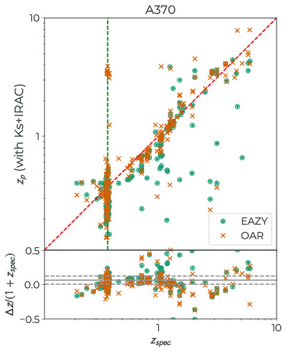
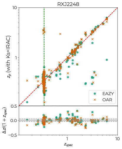
Figure 1: Comparison of the A370 (left) and RXJ2248 (right) spectroscopic redshifts compiled from the literature by Shipley et al. (2018) vs. photometric redshifts derived in this work using full photometry (HST+VLT/HAWK-I+Spitzer). Circles and crosses present the two methods used for photometric redshifts, EAZY and OAR, respectively. The bottom panels show the residuals, solid and dashed line are the median and standard deviation respectively (see also Table 1). The increased ICL component of A370 likely leads to the lower accuracy/precision of the photometric redshifts for both methods.

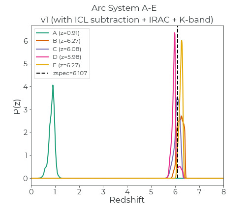
Figure 2: Comparison of our estimates of the photometric redshifts distribution for a quintuply imaged system at $z_{\rm spec}=6.107$ behind RXC J2248.7$-$4431 (Karman et al. 2015, Schmidt et al. 2017). Plotted are photometric redshift probability distributions using ICL subtraction and full photometry (HST+VLT/HAWK-I+Spitzer) for each of the images A-E. Their spectroscopic redshifts are given by a dashed line, and best photometric redshifts are indicated in the legend. Image A is located very close to the core of the cluster and its photometry is less precise (Schmidt et al. 2017).

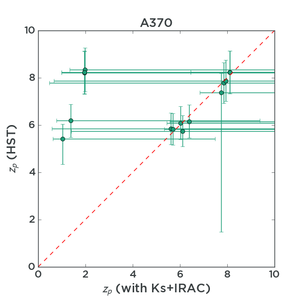
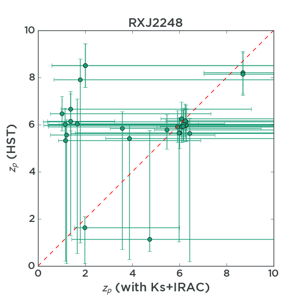
Figure 3: Comparison of the redshifts for the high redshift dropouts behind A370 (left) and RXJ2248 (right) from Ishigaki et al. (2018). Plotted are photometric redshifts and errors from Ishigaki et al. (2018) using only HST data vs. EAZY redshifts and 95% confidence limits derived in this work using full photometry (HST+VLT/HAWK-I+Spitzer).

Table 1: Photomeric redshift accuracy. Listed are biweight location of the $(z_{\rm spec}-z_{\rm phot})/(1+z_{\rm spec})$, median absolute deviation $\sigma_{\frac{\Delta z}{1+z_{\rm spec}}}$ and number of outliers defined as $\left|(z_{\rm spec}-z_{\rm phot})/(1+z_{\rm spec})\right|>0.15$.

Cluster	Sample	$\left<\frac{\Delta z}{1+z_{\rm spec}}\right>$	$\sigma_{\frac{\Delta z}{1+z_{\rm spec}}}$	Outliers
A370 EAZY	202	0.06	0.05	$21\%$
A370 OAR		0.02	0.07	$24\%$
RXJ2248 EAZY	210	0.0006	0.04	$9\%$
RXJ2248 OAR		0.005	0.04	$9\%$

The main high level science products that make rich data sets such as those in the HFFs even more useful for the community are photometric catalogues that combine all the available imaging in a consistent manner. Photometric catalogues for the first four clusters have been published and provided to the community (Merlin et al. 2016a, Castellano et al. 2016, Di Criscienzo et al. 2017). In collaboration with the ASTRODEEP team, we provide equivalent catalogues for the last two HFF clusters Abell 370 (hereafter A370) and RXC J2248.7$-$4431 (hereafter RXJ2248) using almost identical methods to those employed for the first four HFF clusters (Merlin et al. 2016a, Castellano et al. 2016, Di Criscienzo et al. 2017, Santini et al. 2017). Though catalogues have also been published by Shipley et al. (2018) for all six HFF clusters, the catalogues presented here use a different methodology for measuring photometry, photometric redshifts, and stellar properties; therefore they provide independent and complementary measurements. We use the spectroscopic catalogues assembled by Shipley et al. (2018), as well as perform some high-level comparisons throughout the paper.

In this paper we describe the new catalogues and investigate the utility of the longer wavelength data by investigating the high-redshift dropout candidates. In addition, we also perform comparison of photometric redshifts with known spectroscopic redshifts, including for multiply imaged sources. Finally, we combine data for all six HFF clusters and explore stellar properties of a large sample of 20,000 galaxies. The paper is structured as follows. In Section 2 we present the data used to generate the catalogues and in Section 3 we describe the steps taken to generate these catalogues and their public release. In Section 4 we present the main science results that include redshift comparisons and measurements of stellar properties. We summarize in Section 5 and give the location of publicly released catalogues in Appendix A.

Throughout the paper we assume a $\Lambda$CDM concordance cosmology with $\Omega_{\rm m}=0.3$, $\Omega_{\Lambda}=0.7$, and Hubble constant $H_{0}=70{\rm\ kms^{-1}\>\mbox{Mpc}^{-1}}$ (Komatsu et al. 2011, Riess et al. 2011). Coordinates are given for the epoch J2000.0, and magnitudes are in the AB system.

2 Data

A370 and RXJ2248 are the final two clusters from the HFF campaign. They were imaged with 140 orbits each in three optical (ACS; F435W, F606W, F814W) and four near infra-red (WFC3; F105W, F125W, F140W, F160W) bands in one pointing. We use the HST data available here, in particular we use version 1.0 epochs 1 and 2 in both cases. In order to combine it with Spitzer data we use images drizzled to $0.06\arcsec/{\rm pixel}$ scale. We use the Spitzer data available here as well as tools that were developed for our SURFSUP program (Bradač et al. 2014, Ryan et al. 2014, Huang et al. 2016a; HFF postdates SURFSUP and only MACS J1149.5$+$2223 and MACS J0717$+$3745 data is in common). Finally we also use HAWK-I data from the VLT/ESO program 092.A-0472(A) (PI Brammer, Brammer et al. 2016) and spectroscopic data from Keck/LRIS, VLT/MUSE, VLT/FORS2, Magellan/LDSS3, Keck/Deimos, and HST/GRISM (GLASS program) collated by Shipley et al. (2018) using various literature sources (Brammer et al. 2019, in prep., Lagattuta et al. 2017, Treu et al. 2015, Karman et al. 2017, Diego et al. 2016, Richard et al. 2014).

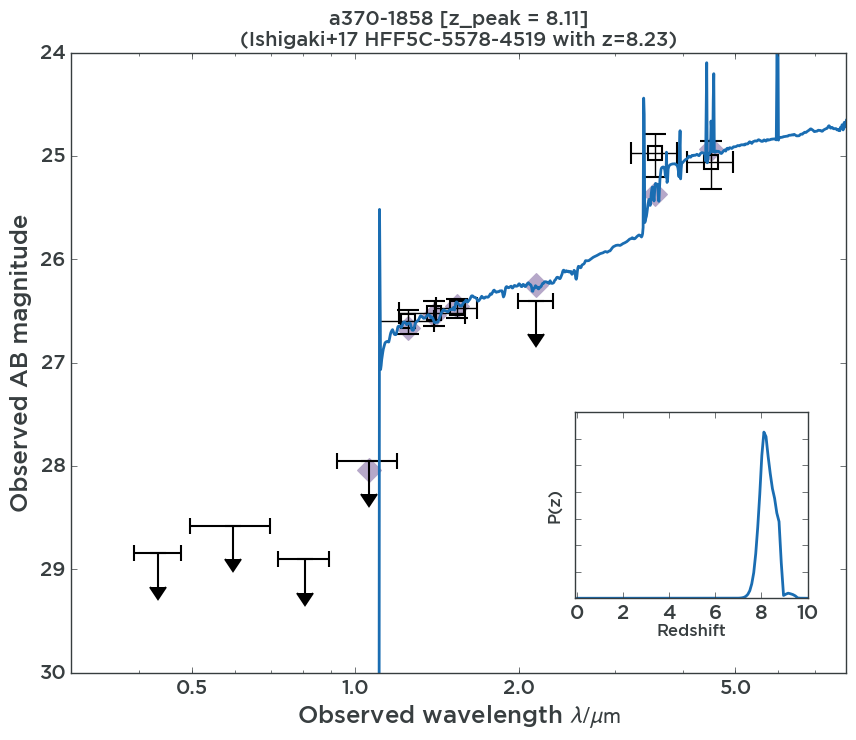
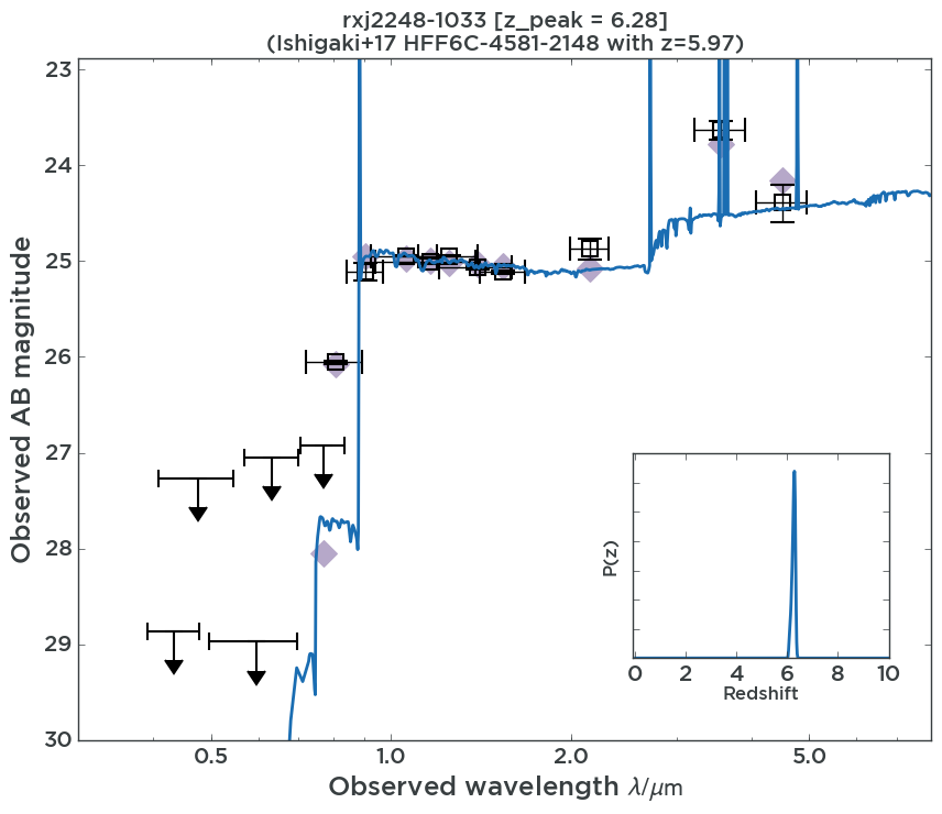
Figure 4: Examples of spectral energy distribution (observed AB magnitude vs wavelength) and redshift probability distribution (insets) plots for two objects behind A370 (left) and RXJ2248 (right). Points with error bars show multiband photometric data from this work, line shows the best fit template as fit by EAZY and diamonds represent the expected magnitudes based on this template. Both objects are selected to be high redshift galaxies based on their photometry. In addition, both show IRAC detections indicating either strong nebular emission lines or old stellar populations based on their Balmer breaks.

3 Data Analysis and Catalogues

Our data analysis closely follow the procedures outlined in Merlin et al. (2016a), Castellano et al. (2016), Di Criscienzo et al. (2017), Huang et al. (2016b). For completeness, we briefly outline the procedure below.

To improve detection of faint sources in the cluster, we start by modeling and subtracting diffuse intra-cluster light (ICL) in the HST F160W images using the procedure outlined in Merlin et al. (2016a). This is to remove the spatially varying background in the cluster field that complicates photometry (especially for faint, high-redshift sources that we are targeting). We first mask out bright pixels above 8 times the estimated sky level, and then we use GALFIT (Peng et al. 2011) to model the ICL with one component using Ferrer profiles (Giallongo et al. 2014). The initial guesses for the centroid, central surface brightness, and truncation radius are the cluster center (brightest cluster galaxy), $22\mbox{mag/arcsec}^{2}$, and $30\arcsec$, respectively. The purpose of fitting ICL with Ferrer profile is not to carefully characterize ICL (as in, e.g., Morishita et al. 2017b), but rather to obtain images with more uniform background for photometry.

After we obtain an initial estimate of the ICL component, we fix the ICL parameters and use GALAPAGOS (Barden et al. 2012) and GALFIT to model bright cluster galaxies. This step involves a first run of SExtractor (Bertin & Arnouts 1996) to obtain initial guesses for GALFIT for each bright cluster member as well as adding secondary GALFIT components to each cluster member to better model their light profiles (especially around the cores). This step is particularly important for A370; because of its low redshift compared with other clusters in the HFF sample, its cluster members occupy a larger fraction of the field of view and make detecting background high-redshift sources more challenging. After satisfactory models of bright cluster members are obtained, we refine the ICL component by relaxing its centroid position, central surface brightness, and truncation radius. Although subtracting ICL and bright cluster members does not improve the signal-to-noise ratios of faint sources, it makes detecting them using SExtractor easier by reducing gradients in local background. It is also a lot easier to visually assess the detection of faint sources once ICL and bright cluster members are removed.

After the above process is finished for F160W (our detection image), we repeat the same process for all other HST filters, using the best-fit parameters from the next redder filter as initial guesses. Modeling of ICL and bright cluster members are done separately on IRAC and $K_{s}$ bands because of their lower-resolutions, which requires a different tool (T-PHOT) as explained below.

We extract photometry on the HST images using SExtractor. For the final detection catalogues we use F160W processed images and use SExtractor with a HOT+COLD approach (Galametz et al. 2013). This procedure adopts two different sets of the SExtractor parameters to detect objects at different spatial scale, COLD for bright extended objects and HOT for faint galaxies. We also match the point-spread functions (PSFs) among all HST filters to get consistent colour. To this aim, we identify isolated point sources in each cluster field, and we use the psfmatch task in IRAF to match all HST images to have the same PSF as the F160W band.

To determine the Spitzer-HST and VLT/HAWKI-HST colors we use the template fitting software T-PHOT (Merlin et al. 2015, 2016b). This is necessary, as unlike the PSF between different HST images, the PSF of especially Spitzer/IRAC is much larger ($\sim 2\arcsec$) compared to HST ($\sim 0.1\arcsec$). To prepare the HST images for T-PHOT, we use the public $0.06\arcsec/{\rm pixel}$ scale images. We also edit the astrometric image header values (CRVALs and CRPIXs, see Merlin et al. 2015) to conform to T-PHOT’s astrometric requirements and make sure that HST and Spitzer images are aligned to well within $0.1\arcsec$.

Finally we use T-PHOT to measure the fluxes in the low-resolution image (in our case the IRAC and VLT/HAWK-I Ks images) for all the sources detected in the high-resolution image (in our case with the F160W HST images). T-PHOT does so by constructing a template for each source; it convolves the cutout of each source in the F160W image with a PSF-transformation kernel that matches the F160W resolution to the IRAC resolution. T-PHOT solves the set of linear equations to find the combination of coefficients for each template that most closely reproduces the pixel values in the IRAC image. Finally, all fluxes are collated in our final combined photometric catalogues (see Appendix A).

We determine photometric redshifts using two different photometric redshift codes 1) EAZY (Eazy and Accurate Zphot from Yale, Brammer et al. 2008) and 2) OAR (Osservatorio Astronomico di Roma, Fontana et al. 2000) code. We use EAZY with the Bruzual & Charlot (2003, hereafter BC03) templates. For this procedure we set a minimum allowed photometric uncertainty corresponding to 0.05 mags for the HST and HAWK-I bands and 0.1 mags for the IRAC bands: errors smaller than these values are replaced by the minimum allowed uncertainty to account for the zero-point uncertainties. We use the redshifts that correspond to the maximum likelihood probability in our final solution. We account for dust attenuation internal to the galaxy following the prescription by Calzetti et al. (2000). The templates also include strong nebular emission lines, whose fluxes are determined by the Lyman continuum flux of BC03 models and nebular line ratios from Anders & Fritze-v. Alvensleben (2003).

The OAR photometric redshifts are obtained with the zphot.exe code (Fontana et al. 2000) following the procedure described by Grazian et al. (2006) (see also Dahlen et al. 2013, Santini et al. 2015). Best-fit photo-zs are obtained through a $\chi^{2}$ minimization using SED templates from PEGASE 2.0 (Fioc & Rocca-Volmerange 1997). For this procedure we also set minimum photometry errors as described above. Throughout this work we use EAZY photometric redshifts, except when comparing with the spectroscopic sample where we use both (Sect. 4.1). Note that in neither case do we assume a prior to account for the existence of each cluster, in doing so photometric redshifts at the cluster redshift would improve (Morishita et al. 2017a).

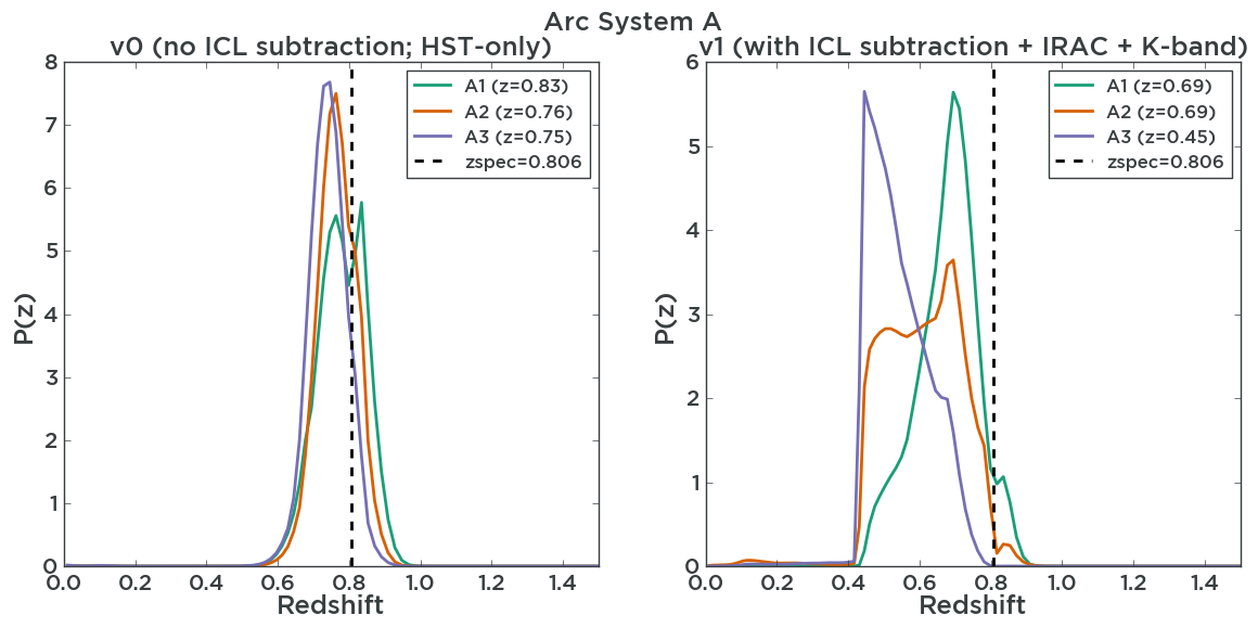
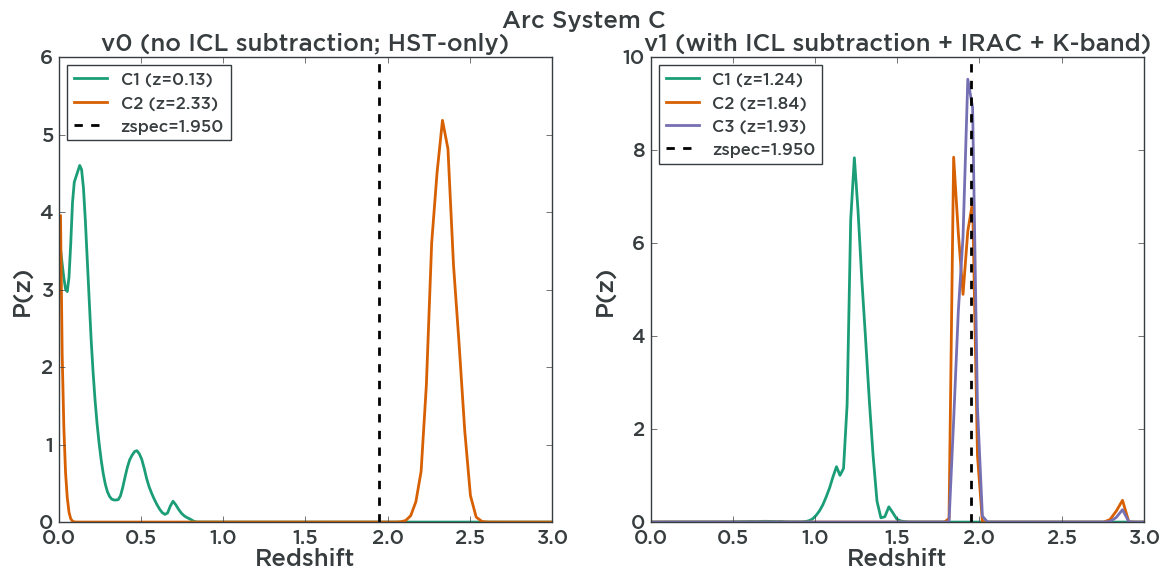
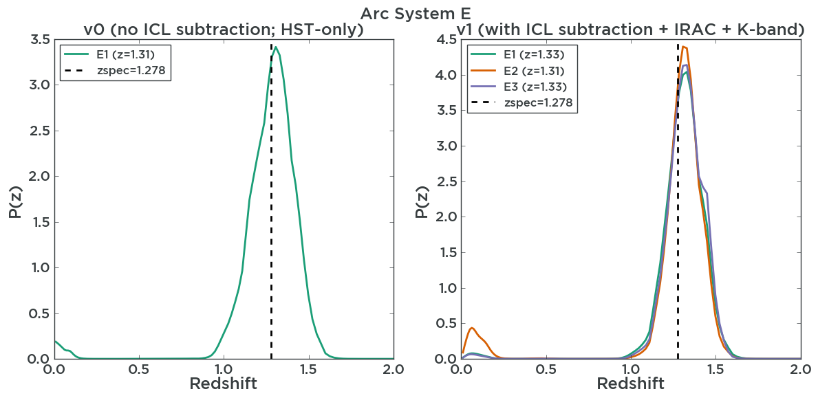
Figure 5: Comparison of the photometric redshifts for the multiply imaged systems behind Abell 370. Plotted are photometric redshift probability distributions using only HST photometry without ICL subtraction and redshifts derived in this work using ICL subtraction and full photometry (HST+VLT/HAWK-I+Spitzer). Three systems with measured spectroscopic redshifts A (top, system 1 in Strait et al. 2018), C (middle, system 3) and E (bottom, system 5) are plotted and their spectroscopic redshifts are given by a dashed line. While ICL subtraction allows us to detect fainter images of the system (case C and E), even with the multiband photometry the photometric redshift solution can still lead to incorrect estimates of the redshift of the system (as is the case for system A, which is located close to the cluster core and its photometry is less reliable).

Galaxy physical properties are computed as described by Castellano et al. (2016) fitting BC03 templates with the zphot.exe code at the previously determined spectroscopic redshift where available or photometric redshift from the EAZY code ($z_{\rm best}$). Only sources with reliable redshifts $z_{\rm best}\geq 0$ that have reliable photometry (no artifacts and coverage in most of the bands) are used. Using OAR photometric redshift does not significantly change the results. For this cursory analysis, to allow for the broadest possible comparison, we adopt a suite of SFHs most commonly employed during the SED process for deep extragalactic surveys. In the BC03 fit we assume exponentially declining star-formation histories (SFHs) with e-folding time $0.1\leq\tau\leq 15.0\mbox{Gyr}$. Note, however, that stellar masses are only mildly sensitive to the choice of the SFH (Santini et al. 2015), and this choice does not significantly affect our results. We assume a Salpeter (1955) initial mass function and we allow both Calzetti et al. (2000) and Small Magellanic Cloud (Prevot et al. 1984) extinction laws. Absorption by the intergalactic medium (IGM) is modeled following Fan et al. (2006). We fit all the sources with stellar emission templates including the contribution from nebular continuum and line emission following Schaerer & de Barros (2009) under the assumption of an escape fraction of ionizing photons $f_{\rm esc}=0.0$ (see also Castellano et al. 2014 for details). SFRs were estimated from UV rest-frame photometry using approach outlined in (Castellano et al. 2012). UV slope $\beta$ was used to obtain the the dust-corrected UV magnitude, which is then used to obtain an SFR estimate with the Kennicutt & Evans 2012 factor. We also release catalogues of these properties as described in the Appendix A.

4 Results

4.1 Comparison with Spectroscopic samples

After the photometric catalogues were finalized, we compared spectrocopic redshifts to photometric redshifts as computed using methodology described above. We did not use spectroscopic redshifts to adjust the imaging zero-points. In addition, the photometry was not optimized for large galaxies (i.e. cluster members, see e.g. Tortorelli et al. 2018), as our primary goal was to study high-redshift galaxies. Spectroscopic redshifts were recently collected by Shipley et al. (2018) using various literature sources. For A370 the catalogues are Brammer et al. (2019, in prep.), Lagattuta et al. (2017), Treu et al. (2015), Richard et al. (2014) and for RXJ2248 they used Brammer et al. (2019, in prep.), Karman et al. (2017), Diego et al. (2016), Treu et al. (2015), Richard et al. (2014). The comparison is given in Figure 1. Overall, the photometric redshift performance is very similar to the performance reported by Shipley et al. (2018), Castellano et al. (2016), Di Criscienzo et al. (2017). The results for the biweight location (a robust statistic for determining the central location of a distribution) of the $(z_{\rm spec}-z_{\rm phot})/(1+z_{\rm spec})$, median absolute deviation and number of outliers defined as $\left|(z_{\rm spec}-z_{\rm phot})/(1+z_{\rm spec})\right|>0.15$ are listed in Table 1. The fraction of catastrophic outliers is higher for A370, likely due to larger ICL contamination. From now on, unless specified otherwise, we will use EAZY photometric redshifts.

4.2 High Redshift Galaxies

One of the main goals of the HFF program was to detect high redshift, highly magnified galaxies. We briefly perform an analysis here to investigate galaxies with secure spectral redshifts at $z>6$. For the $z>6$ population very few spectroscopic redshifts exist. For the two clusters studied in this work we have a total of 2 galaxies with spectroscopic redshifts at $z>6$. These are $z=6.5$ object by Hu et al. (2002) behind A370 and a quintuply imaged system at $z=6.107$ behind RXJ2248 (Karman et al. 2015, Schmidt et al. 2017). For RXJ2248, four images are correctly identified at $z=6.107$ within $\pm 0.2$, while one fails catastrophically and is put at $z\sim 1$ (Fig. 2). The image that fails is located very close to the core of the cluster and its photometry is likely affected. In Shipley et al. (2018) one of the objects also fails (a different one) and is put at $z\sim 4$.

We also looked into the sample from Ishigaki et al. (2018), where high redshift galaxies were selected based on the dropout technique (Steidel et al. 1996), and their photometric redshifts were determined subsequently using only HST data. The dropout technique is based on the photometric detection/non-detection of objects near the Lyman break. As such it does not use rest-frame optical information. The results are shown in Fig. 3. The addition of rest-frame optical data (HST+VLT/HAWK-I+Spitzer) is essential, as it can often identify lower redshift dusty objects for which the break could mimic the Lyman$\alpha$/Lyman-limit break. Hence, we see a non-trivial fraction ($\sim$30-45%) of objects that scatter to lower redshift when such data is added. Spitzer data is especially powerful in this case, as it targets high equivalent width nebular emission lines and/or can detect “old” stellar populations based on the 4000Å break (see Fig. 4 for examples of SED fitting). This not only improves accuracy of redshift determination, but also allows us to better study stellar properties at highest redshifts.

4.3 Multiple Imaged Systems

Another common application of photometric redshifts is to determine redshifts of the multiply imaged systems to be used for strong gravitational lensing and accurate determinations of projected mass distribution and magnification of clusters. This is important for high redshift studies, as stellar masses and SFRs need to be corrected for magnification to obtain intrinsic values (see Sect. 4.4). Erroneous redshifts can significantly bias results (e.g., Treu et al. 2016, Grillo et al. 2016, Remolina González et al. 2018). We look into how well photometric redshifts fulfill this task for the set of multiple images with spectroscopic redshifts. These are some of the more difficult objects on which to perform accurate photometry on. They are often distorted, hence traditional photometry approaches can fail. Our results are shown in Figs. 2, 5. While ICL subtraction allows us to detect fainter images of the system (case C and E in Fig. 5), even with the full multiband photometry the photometric redshift solution can be biased. An important quantity to consider is the angular diameter distance ratio between the source and the lens (deflector) and the observer and the source $D_{\rm ds}/D_{\rm s}$. For a typical lens at redshift $z_{\rm d}=0.5$, this ratio changes by $10\mbox{-}50\%$ for source redshifts of $z_{\rm s}=1.3\mbox{--}0.7$ assuming source redshift error of $\Delta z/(1+z)=0.1$. The error on $D_{\rm ds}/D_{\rm s}$ (if present in the same direction for all multiple images) will then directly translate to the error in normalization of the mass distribution. Therefore, whenever performing lens modeling it is best to obtain a large spectroscopic sample.

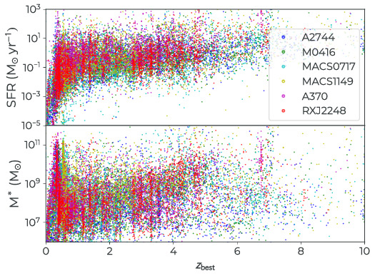
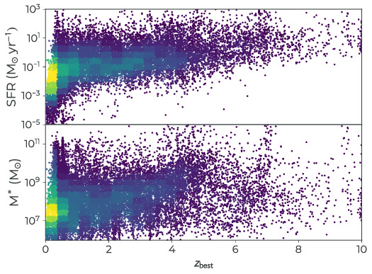
Figure 6: Star Formation Rate (SFR) and stellar mass ($M_{\ast}$) sepparated by cluster (top) and as a hybrid density plot (bottom) as a function of best redshift $z_{\rm best}$. The plots include all six HFF clusters (main pointing, A2744, MACS0416 from Castellano et al. 2016, MACS1149, MACS0717 from Di Criscienzo et al. 2017, and A370, RXJ2248 from this work). Both SFR and $M_{\ast}$ have been corrected for magnification using median magnifications from all submitted lens models as described by Castellano et al. (2016). Gravitational lensing allows galaxies to be detected at stellar masses as low as $10^{7}M_{\odot}$ and intrinsic $\mbox{SFRs}\sim 0.1\mbox{--}1M_{\odot}/\mbox{yr}$ even at the highest redshifts.

4.4 Stellar Properties

Stellar properties of galaxies in all six catalogues (Castellano et al. 2016, Di Criscienzo et al. 2017 and this work) are presented in Figs. 6,7. Each cluster’s main pointing contains $3000-4000$ galaxies with measured properties for a total of $20,000$ objects. In Fig. 6 we show Star Formation Rate (SFR) and stellar mass ($M_{\ast}$) as a function of redshift. Both quantities have been corrected for magnification using median magnifications from version 4 lens models as described by Castellano et al. (2016) (see models and version description here ). It is very encouraging to see that we can target galaxies down to stellar mass of $10^{7}M_{\odot}$ even at the highest redshift (this is similar to the mass of Fornax dwarf spheroidal, Kirby et al. 2013). At intermediate redshifts some stellar mass might be coming from relatively evolved ($\sim 500\mbox{Myr}\mbox{--}1\mbox{Gyr}$) populations due to the lack of rest frame near-IR data and in that case, these low masses should be considered as lower limits. However, at the highest redshifts any contribution from dusty populations is likely to be sub-dominant. Similarly we can detect galaxies down to intrinsic $\mbox{SFRs}\sim 0.1\mbox{--}1M_{\odot}/\mbox{yr}$ at $z>6$.

Fig. 7 shows a plot of a specific star formation rate (sSFR) as a function of $z_{\rm best}$. These results are independent of lens magniffication. However, it is the magnification which enables us to obtain a more complete sample down to lower stellar masses. The maximum values of $\mbox{sSFR}=10^{2}\mbox{Gyr}^{-1}$ are indicative of the youngest stellar population models we use ($10\mbox{Myr}$). We only plot galaxies with $M_{\ast}=10^{9.5}\mbox{--}10^{10}M_{\odot}$ as is often done in the literature (e.g., Santini et al. 2017) and $68\%$ confidence limits with median value in each bin. The results are consistent with e.g. Tasca et al. (2015) at $2<z<5$; though Tasca et al. (2015) sample includes only galaxies with spectroscopic redshifts and thus has a cleaner sample.

Qualitatively at high redshifts our results are affected by incompleteness in stellar mass (we are less likely to detect low stellar mass objects). Since F160W traces rest-frame UV light, only high SFR objects will enter our sample. In order to estimate the incompleteness in SFR we would need a complete sample of galaxy colours at high redshifts to estimate the full range of SFRs; such a sample is not available. In addition, selecting galaxies based on rest frame optical data is not possible at present due to the relatively shallow depth and large PSF of the Spitzer data. The measurement errors also increase for high redshift and faint sources, which could lead to the Eddington bias. As shown by Santini et al. (2017), correcting for the Eddington bias would increase sSFR at $z>3$. Finally, as with any sSFR measurement the systematic uncertainty of measuring SFR (e.g., lack of direct tracers such as dust corrected $H\alpha$, uncertainties due to unknown IMF) and $M_{*}$ (e.g., uncertainties due to unknown IMF) using photometry remain. The detailed explorations of sSFR at highest redshifts will thus have to await the launch of JWST.

5 Conclusions

In this paper we present and publicly release photometric catalogues of two HFF clusters, Abell 370 and RXC J2248.7$-$4431. The catalogues include HST, HAWK-I/Ks band and Spitzer data. We measure photometric redshifts for all sources and compare them to spectroscopic data from the literature. Comparison shows a reasonable agreement with $\sigma_{\Delta z/(1+z_{\rm spec})}\sim 0.05$ and an outlier fraction of $10-20\%$. The fraction is higher for A370, likely due to larger ICL contamination. We have also explored the accuracy of photometric redshifts for strongly lensed systems and conclude that their errors can cause a significant bias in lens modeling.

Finally, we explore the stellar properties of galaxies using samples from all 6 HFF clusters, containing 20,000 galaxies. The magnification from a foreground cluster allows for the detection of objects with stellar mass $M_{\ast}\gtrsim 10^{7}M_{\odot}$ and intrinsic SFRs$\sim 0.1\mbox{-}1M_{\odot}/\mbox{yr}$ at $z>6$. Photometric redshifts, magnification values, rest-frame properties and supporting information are all made publicly available as described in the Appendix A.

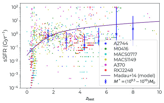
Figure 7: sSFR as a function of redshift $z_{\rm best}$ for all 6 HFF clusters (main pointing, A2744, MACS0416 from Castellano et al. 2016, MACS1149, MACS0717 from Di Criscienzo et al. 2017, and A370, RXJ2248 from this work). Also plotted is the theoretical model from Madau & Dickinson (2014) and binned data points with errorbars. Only galaxies with $M_{\ast}=10^{9.5}-10^{10}M_{\odot}$ are plotted and considered in the binning of the data as is often done in the literature. The maximum values of $\mbox{sSFR}=10^{2}\mbox{Gyr}^{-1}$ are indicative of the youngest stellar population models we use ($10\mbox{Myr}$). Note that sSFR is independent of magniffication.

Appendix A Public release of the Catalogues

All the catalogues and derived quantities described in this paper are publicly released and can be obtained from these urls.^, Photometric redshift catalogues contain all the photometry as described in Sect. 3. These catalogues also contain photometric redshift properties using EAZY (Brammer et al. 2008).

Stellar properties catalogues contain the same information as catalogues released by (Castellano et al. 2016, Di Criscienzo et al. 2017). In particular::

• ID: identification number that matches the number in the input photometric catalogues.

• ZBEST: corresponds to the reference photo-z value used in fitting stellar properties ($z_{\rm best}$). We use spectroscopic redshift where available, and photometric redshift from EAZY otherwise. Sources for which the photo-z run did not converge to a solution or have unreliable photometry are set to $ZBEST=-1.0$.

• MAGNIF: median magnification from all the models with version 4 data from this url${}^{\ref{fn:lm}}$.

• CHI2_NEB: $\chi^{2}$ of the SED fitting with stellar plus nebular templates at redshift fixed to ZBEST.

• MSTAR_NEB, MSTAR_MIN_NEB, MSTAR_MAX_NEB: stellar mass ($10^{9}M_{\odot}$) estimated from stellar plus nebular fits.

• SFR_NEB, SFR_MIN_NEB, SFR_MAX_NEB: star-formation rate ($M_{\odot}/\mbox{yr}$) estimated from the stellar plus nebular fits.

• CHI2_NONEB, MSTAR_NONEB, MSTAR_MIN_NONEB, MSTAR_MAX_NONEB, SFR_NONEB, SFR_MIN_NONEB, SFR_MAX_NONEB similar to the quantities above, but SED fitting was performed using stellar templates only. Throughout the paper we quote all results from SED fitting using stellar plus nebular templates, but add these values to the catalog for convenience.

References

- Anders & Fritze-v. Alvensleben (2003) Anders P., Fritze-v. Alvensleben U., 2003, A&A, 401, 1063
- Barden et al. (2012) Barden M., Häußler B., Peng C. Y., McIntosh D. H., Guo Y., 2012, MNRAS, 422, 449
- Bertin & Arnouts (1996) Bertin E., Arnouts S., 1996, A&AS, 117, 393
- Bradač et al. (2014) Bradač M., et al., 2014, ApJ, 785, 108
- Brammer et al. (2008) Brammer G. B., van Dokkum P. G., Coppi P., 2008, ApJ, 686, 1503
- Brammer et al. (2016) Brammer G. B., et al., 2016, ApJS, 226, 6
- Brammer et al. (2019) Brammer G. B., et al., 2019, Grism analysis of the Hubble Frontier Fields, in prep.
- Bruzual & Charlot (2003) Bruzual G., Charlot S., 2003, MNRAS, 344, 1000
- Calzetti et al. (2000) Calzetti D., Armus L., Bohlin R. C., Kinney A. L., Koornneef J., Storchi-Bergmann T., 2000, ApJ, 533, 682
- Castellano et al. (2012) Castellano M., et al., 2012, A&A, 540, A39
- Castellano et al. (2014) Castellano M., et al., 2014, A&A, 566, A19
- Castellano et al. (2016) Castellano M., et al., 2016, A&A, 590, A31
- Dahlen et al. (2013) Dahlen T., et al., 2013, ApJ, 775, 93
- Di Criscienzo et al. (2017) Di Criscienzo M., et al., 2017, A&A, 607, A30
- Diego et al. (2016) Diego J. M., Broadhurst T., Wong J., Silk J., Lim J., Zheng W., Lam D., Ford H., 2016, MNRAS, 459, 3447
- Fan et al. (2006) Fan X., Carilli C. L., Keating B., 2006, ARA&A, 44, 415
- Fioc & Rocca-Volmerange (1997) Fioc M., Rocca-Volmerange B., 1997, A&A, 326, 950
- Fontana et al. (2000) Fontana A., D’Odorico S., Poli F., Giallongo E., Arnouts S., Cristiani S., Moorwood A., Saracco P., 2000, AJ, 120, 2206
- Galametz et al. (2013) Galametz A., et al., 2013, ApJS, 206, 10
- Giallongo et al. (2014) Giallongo E., et al., 2014, ApJ, 781, 24
- Grazian et al. (2006) Grazian A., et al., 2006, A&A, 449, 951
- Grillo et al. (2016) Grillo C., et al., 2016, ApJ, 822, 78
- Hu et al. (2002) Hu E. M., Cowie L. L., McMahon R. G., Capak P., Iwamuro F., Kneib J.-P., Maihara T., Motohara K., 2002, ApJ, 568, L75
- Huang et al. (2016a) Huang K.-H., et al., 2016a, ApJ, 817, 11
- Huang et al. (2016b) Huang K.-H., et al., 2016b, ApJ, 823, L14
- Ishigaki et al. (2018) Ishigaki M., Kawamata R., Ouchi M., Oguri M., Shimasaku K., Ono Y., 2018, ApJ, 854, 73
- Karman et al. (2015) Karman W., et al., 2015, A&A, 574, A11
- Karman et al. (2017) Karman W., et al., 2017, A&A, 599, A28
- Kennicutt & Evans (2012) Kennicutt R. C., Evans N. J., 2012, ARA&A, 50, 531
- Kirby et al. (2013) Kirby E. N., Cohen J. G., Guhathakurta P., Cheng L., Bullock J. S., Gallazzi A., 2013, ApJ, 779, 102
- Komatsu et al. (2011) Komatsu E., et al., 2011, ApJS, 192, 18
- Lagattuta et al. (2017) Lagattuta D. J., et al., 2017, MNRAS, 469, 3946
- Madau & Dickinson (2014) Madau P., Dickinson M., 2014, ARA&A, 52, 415
- Merlin et al. (2015) Merlin E., et al., 2015, A&A, 582, A15
- Merlin et al. (2016a) Merlin E., et al., 2016a, A&A, 590, A30
- Merlin et al. (2016b) Merlin E., et al., 2016b, A&A, 595, A97
- Morishita et al. (2017a) Morishita T., et al., 2017a, ApJ, 835, 254
- Morishita et al. (2017b) Morishita T., Abramson L. E., Treu T., Schmidt K. B., Vulcani B., Wang X., 2017b, ApJ, 846, 139
- Peng et al. (2011) Peng C. Y., Ho L. C., Impey C. D., Rix H.-W., 2011, GALFIT: Detailed Structural Decomposition of Galaxy Images, Astrophysics Source Code Library (ascl:1104.010)
- Postman et al. (2012) Postman M., et al., 2012, ApJS, 199, 25
- Prevot et al. (1984) Prevot M. L., Lequeux J., Maurice E., Prevot L., Rocca-Volmerange B., 1984, A&A, 132, 389
- Remolina González et al. (2018) Remolina González J. D., Sharon K., Mahler G., 2018, ApJ, 863, 60
- Richard et al. (2014) Richard J., et al., 2014, MNRAS, 444, 268
- Riess et al. (2011) Riess A. G., et al., 2011, ApJ, 730, 119
- Ryan et al. (2014) Ryan Jr. R. E., et al., 2014, ApJ, 786, L4
- Salpeter (1955) Salpeter E. E., 1955, ApJ, 121, 161
- Santini et al. (2015) Santini P., et al., 2015, ApJ, 801, 97
- Santini et al. (2017) Santini P., et al., 2017, ApJ, 847, 76
- Schaerer & de Barros (2009) Schaerer D., de Barros S., 2009, A&A, 502, 423
- Schmidt et al. (2017) Schmidt K. B., et al., 2017, ApJ, 839, 17
- Shipley et al. (2018) Shipley H. V., et al., 2018, ApJS, 235, 14
- Steidel et al. (1996) Steidel C. C., Giavalisco M., Pettini M., Dickinson M., Adelberger K. L., 1996, ApJ, 462, L17+
- Strait et al. (2018) Strait V., et al., 2018, ApJ, 868, 129
- Tasca et al. (2015) Tasca L. A. M., et al., 2015, A&A, 581, A54
- Tortorelli et al. (2018) Tortorelli L., et al., 2018, MNRAS, 477, 648
- Treu et al. (2015) Treu T., et al., 2015, ApJ, 812, 114
- Treu et al. (2016) Treu T., et al., 2016, ApJ, 817, 60